Atmospheric Temperature Effect in secondary cosmic rays observed with a two square meter ground-based detector

Abstract

A high resolution 2 m² tracking detector, based on timing Resistive Plate Chamber (tRPC) cells, has been installed at the Faculty of Physics of the University of Santiago de Compostela (Spain) in order to improve our understanding of the cosmic rays arriving at the Earth’s surface. Following a short commisioning of the detector, a study of the atmospheric temperature effect of the secondary cosmic ray component was carried out. A method based on Principal Component Analysis (PCA) has been implemented in order to obtain the distribution of temperature coefficients, $W_{T}(h)$, using as input the measured rate of nearly vertical cosmic ray tracks, showing good agreement with the theoretical expectation. The method succesfully removes the correlation present between the different atmospheric layers, that would be dominant otherwise. We briefly describe the initial calibration and pressure correction procedures, essential to isolate the temperature effect. Overall, the measured cosmic ray rate displays the expected anticorrelation with the effective atmospheric temperature, through the coefficient $\alpha_{T}=-0.279\pm 0.051$ %/K. Rates follow the seasonal variations, and unusual short-term events are clearly identified too.

Earth and Space Science

CRETUS Institute, Group of Nonlinear Physics, Faculty of Physics, University of Santiago de Compostela, Spain Instituto Galego de Física de Altas Enerxías, Faculty of Physics, University of Santiago de Compostela, Spain

Irma Riádigosirma.riadigos@usc.es

Atmospheric temperature effect isolated with timing resistive plate chambers for the first time

Extraction of temperature coefficients versus atmosphere depth through principal component regression and comparison with theoretical expectation

Seasonal and occasional variations for the cosmic ray flux observed, showing consistency with earlier Global Muon Detector Network results

1 Introduction

Cosmic rays (c.r.) are messengers from outer space that provide valuable information for different research areas, such as space weather, high energy physics and cosmology [Pierre Auger Collaboration (2015), Hayashi . (2005)]. Specifically, ground-based instruments give us the chance to study the products of the interactions between primary cosmic rays and the nuclei in the atmosphere. These products consist of secondary particles that traverse the atmosphere carrying information about its inner structure, as in a radiography, providing information about its properties. Secondary muons, in particular, are affected by atmospheric pressure and temperature. These induce local modifications of the atmospheric density and its depth, thereby changing the balance between particle production, absorption and decay, affecting the muon rates at ground [Dorman (2004)]. Since modern muon detectors are mostly committed to the study of solar activity and other astrophysical phenomena, such effects are regularly removed with simple techniques, as part of a calibration procedure [De Mendonca . (2013)]. Our work is concerned with a deeper comprehension of such atmospheric effects.

The rates of c.r. measured at the Earth’s surface vary according to changes in several atmospheric conditions, chiefly the pressure at ground level and the temperature profile of the atmosphere. The pressure (or barometric) effect arises mainly due to the absorption of the radiation in the atmosphere through energy loss. The more the pressure, the more air mass to traverse. Therefore, secondary c.r. particles are more efficiently absorbed and, consequently, the measured rates are modulated in anticorrelation with the ground-level pressure. In detail, the mass increase is associated with a larger height of the air column, that modifies the decay probabilities of the particles involved, implying a non-negligible (but sub-dominant) contribution to the main negative correlation [Sagisaka (1986)].

In the absence of variations in the ground-level pressure, the modification of the local density of the air column as a result of temperature variations modifies c.r. rates as well. This so-called ‘temperature effect’ is the result of two contributions: the interaction (positive correlation) and decay (negative correlation) of secondary particles through the atmosphere. Muons ($\mu^{+/-}$), that are the dominant c.r. particles at ground level, originate mainly from the decay of charged pions and kaons ($\pi^{+/-},\textnormal{K}^{+/-}$). Since an increase in temperature reduces the atmospheric density, causing a reduction in the interaction probability, more pions and kaons will decay and produce more muons. Muons, unlike their parents, are highly penetrating, and small changes in their interaction probability leave their behaviour largely unaffected. As a result, the surface rates increase with increasing temperature, creating a positive effect. The negative effect is related to the muon decay itself. Because the atmosphere also expands when the temperature increases, muons have to travel further to reach the surface before they decay. As a result, the surface rates decrease. Importantly, in case of high-energy particles, the positive effect dominates because of time dilation in the muon reference frame. This relativistic effect causes energetic muons to effectively live longer, so their decay probability is reduced. For low energies, on the other hand, the dominant effect is negative. A practical way to ‘increase’ the particle energy is to measure the c.r. rates underground, thus allowing to study the temperature effect as a function of the rock overburden (e.g., [Abrahao . (2017)]).

The temperature effect can be nearly one order of magnitude smaller than its pressure counterpart, enforcing a much better control on systematic effects of instrumental origin and high statistics (detector size) in the first place. A precise estimate of the atmospheric temperature effect involves an implementation of the ‘integral method’, which requires, on the one hand, knowing the temperature profiles above the detector and, on the other hand, knowing the distribution of temperature coefficients ($W_{T}$), the latter accessible by theoretical means [Dmitrieva . (2011)]. Given that the detector used in this work was conceived to potentially make use of both the soft (electron) and hard (muon) cosmic ray component, the temperature coefficients (calculated for muons) are not known a priori. As discussed afterwards, the effect of the material overburden can not be completely neglected, nor easily characterized, either.

The main purpose of this work is to experimentally obtain the temperature coefficients for secondary cosmic rays at ground, resorting to a technology not used previously in these kind of studies. We will show how, despite the much higher dark rates customary of gaseous detectors as compared to plastic scintillators, two $\sim 2$ m² planes of timing Resistive Plate Chambers (tRPCs) operating at ground level are sufficient to isolate the temperature effect, a fact that results largely from the superb timing characteristics of the device.

2 The Muon Telescope (MT)

The tRPC technology was introduced to particle physics back in 2000 as a byproduct of the R&D program of the ALICE experiment at the Large Hadron Collider [Fonte . (2000)]. Indeed, tRPCs have been adopted already for the study of high energy cosmic rays by the EEE collaboration [Abbrescia . (2013)], but no study on the temperature effect has been reported by the collaboration yet. tRPCs represent a family of non-proportional gaseous detectors, generally characterized by the use of thin sub-mm gas gaps operated in ‘fast’ well-quenched gas mixtures at very high electric fields (up to $\sim$ 150 kV/cm). Stability of operation requires the use of insulating materials with high surface quality, something conventionally achieved through soda-lime glass. tRPCs can make an optimal use of the multi-gap technique [Cerrón Zeballos . (1996)], that allows for the systematic stacking of several gas gaps, in order to achieve time resolutions down to 20 ps in special configurations [An . (2008)]. In fact, tRPCs have recently demonstrated the capability of reaching 60 ps on $2\times 2$ m² areas, with a modest number of electronic readout channels around 160, and a position resolution at the cm-scale [Watanabe . (2019)].

At the University of Santiago de Compostela (Spain), a medium-size tRPC detector (1.2 $\times$ 1.5 m²) with a space and time resolution of $\sigma_{x,y}\sim 3$ cm and $\sigma_{t}\sim 300$ ps, respectively, has been installed circa 2014 [Blanco . (2014)]. It is named TRAGALDABAS (TRAsGo for the AnaLysis of the nuclear matter Decay, the Atmosphere, the earth B-Field And the Solar activity), and it has been designed and built at LIP-workshops (e.g., [Abreu . (2018)]). The angular resolution with its present vertical layout is 2-3^∘ and the maximum zenith angle of the accepted tracks is close to 50^∘ (Figure 1a). Unlike other cosmic ray detectors, TRAGALDABAS has a relatively small active area of 1.8 m². For comparison, the MuSTAnG detector [Hippler . (2008)] had a surface of 4 m² and all four telescopes of the Global Muon Detector Network (GMDN) extend over around 15-30 m² [Rockenbach . (2014)].

Figure 1: (a) Drawing of the muon telescope at Santiago de Compostela, showing the tRPC layout with some illustrative examples of different particle interactions. In the present analysis only the T2 and T4 RPC planes are used. (b) Inner view of the detector.

The MT consists of four RPC planes with a total height of 1.8 m (Figure 1a). Each plane’s inner design is based on three plates of 2 mm glass with a 1 mm gas gap interleaved, placed inside a gas-tight acrylic box. Tetrafluoroethane, a type of freon (R134a, CF₃CH₂F), is used as the active medium, at a very low flow, just sufficient to keep the detector efficiency constant over time. The external sides of the outer gas plates are covered with a semi-conductive coating to which a $\pm$ 5600 V high voltage is applied. Electrical pick-up signals, stemming from the avalanches produced in the gas upon the passage of a charged particle, are induced in some of the 120 copper pads placed outside of the acrylic box (Figure 1b). Those signals are processed with fast $\sim 1$ GHz BW electronics [Belver . (2010)] and, if above an adjustable threshold, a digital LVDS signal is produced, marking the passage of the particle (we will refer to the associated pad and plane as ‘fired’). A flexible trigger condition can be formed for any number of fired planes and pad multiplicity per plane, a digital signal formed, correspondingly, and sent to the acquisition in order to store the c.r. candidate. The telescope is placed at $\sim$260 m above sea level, $42^{\circ}$52’N $8^{\circ}$33’W, at a geomagnetic rigidity cutoff of $\sim$5.5 GV and in the first floor of a two-story building. It is running since 2015 with a room temperature stable at 20 $\pm$ 1^∘C.

It is important to note that, except in special configurations (e.g. [Margato . (2019)], [Blanco . (2015)]), RPC detectors have intrinsically a very low detection efficiency for neutrons below 10 MeV, not exceeding 0.1%. Moreover, neither the products from neutron interactions nor electrons from neutron decay at these energies can traverse a second detection plane, as required in present analysis. Hence, if assuming a typical albedo neutron flux of $\sim$1 kHz/cm² [Hubert . (2016)], the detector can be effectively considered as neutron-blind, for the purposes of present analysis.

3 Input data and processing

We report here data from the commissioning phase and early physics run (from October 2015 to January 2017), where only two detector planes, stacked over a height of 120 cm, were used (T2 and T4 in Figure 1a). A trigger condition was defined as ‘at least one fired pad per plane, in time coincidence’. During data analysis, a standard equalization is performed in an automatic way, aimed at the correction of the channel-by-channel variations in the time offsets and signal amplification (along the lines of [Kornakov (2014)]). Provided both charge and time information are stored for each pad, noise signals (displaying zero-charge) can be removed in the next processing step. Finally, ‘particle tracks’ are formed by combinatorialy matching the fired pads in both planes with a velocity compatible with the speed of light, within a $3$-$\sigma_{t}$ interval, being $\sigma_{t}$ the time resolution of the detector. This produces the final data sample ready for physics analysis, where any instrumental effects should be greatly minimized. We use in this work a data sub-sample, corresponding to events with a single track (multiplicity $M=1$), and a zenith angle $\theta$ lower than 13^∘. The former condition means that only cases with one fired pad per plane have been considered.

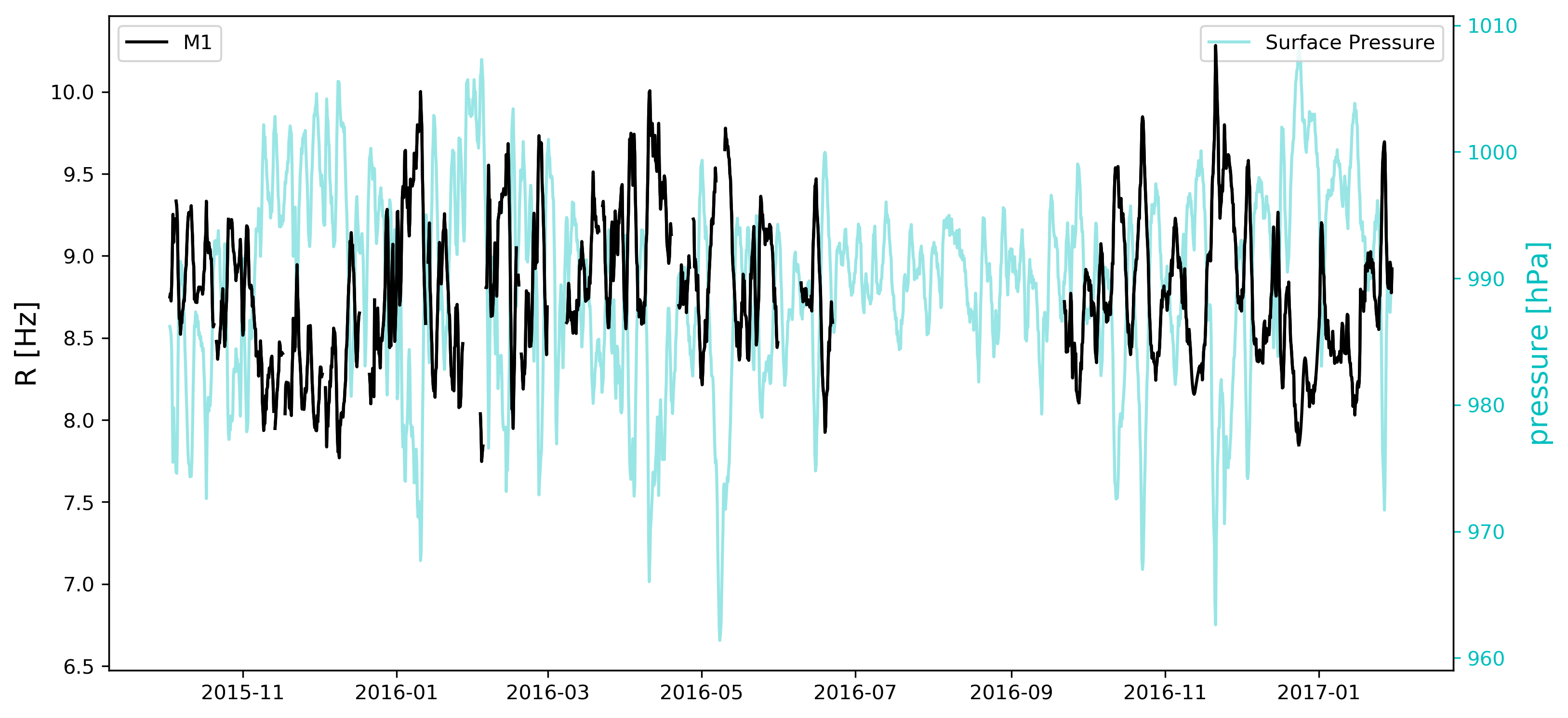
Figure 2: Cosmic ray rate for single vertical tracks as observed with the muon telescope (black curve) and ground-level pressure (blue curve).

The complete data taking period, displayed in Figure 2, may be conveniently divided in three phases:

• From October 2015 to June 2016. During this first period the detector was run semi-autonomously (several interventions were needed) and problems related to faulty front-end electronics and high voltage instabilities were observed.

• From June 2016 to October 2016. Maintenance work was carried out, the faulty electronics modules were replaced, and an on-line monitor developed.

• From October 2016 to January 2017. The detector run in stable conditions, in a fully autonomous way.

Figure 3: Examples of ERA-INTERIM atmospheric temperature profiles for Santiago de Compostela, summer (1 July 2016) and winter (1 January 2017).

Concerning the atmospheric variables, the vertical temperature profiles were retrieved from the European Centre for Medium-Range Weather Forecast (ECMWF) reanalysis, ERA-Interim [Dee . (2011)], for the 1979-2017 period, at 37 isobaric levels (1000, 975, 950, 925, 900, 875, 850, 825, 800, 775, 750, 700, 650, 600, 550, 500, 450, 400, 350, 300, 250, 225, 200, 175, 150, 125, 100, 70, 50, 30, 20, 10, 7, 5, 3, 2, 1 hPa), with a horizontal spatial resolution of $0.125^{\circ}$ and a temporal resolution of 6 h. Two exemplary profiles for summer and winter are shown in Fig. 3.

4 Analysis of Atmospheric Effects

As mentioned before, several methods can be used to take into account the temperature effect of secondary cosmic ray particles in the atmosphere [Blackett (1938), Berkova . (2011), Dorman (2004), Duperier (1949), Sagisaka (1986)]. The integral method has been shown to be one of the most precise in most of the muon telescopes [De Mendonça . (2016), Dmitrieva . (2013)] but it requires knowing the distribution of the temperature coefficients in the atmosphere, $W_{T}(h)$. These can be theoretically calculated for different threshold energies, zenith and azimuth angles of incidence [Dmitrieva . (2011)], or extracted from c.r. data [Yanchukovsky  Kuzmenko (2018)]. In this work we compare both approaches.

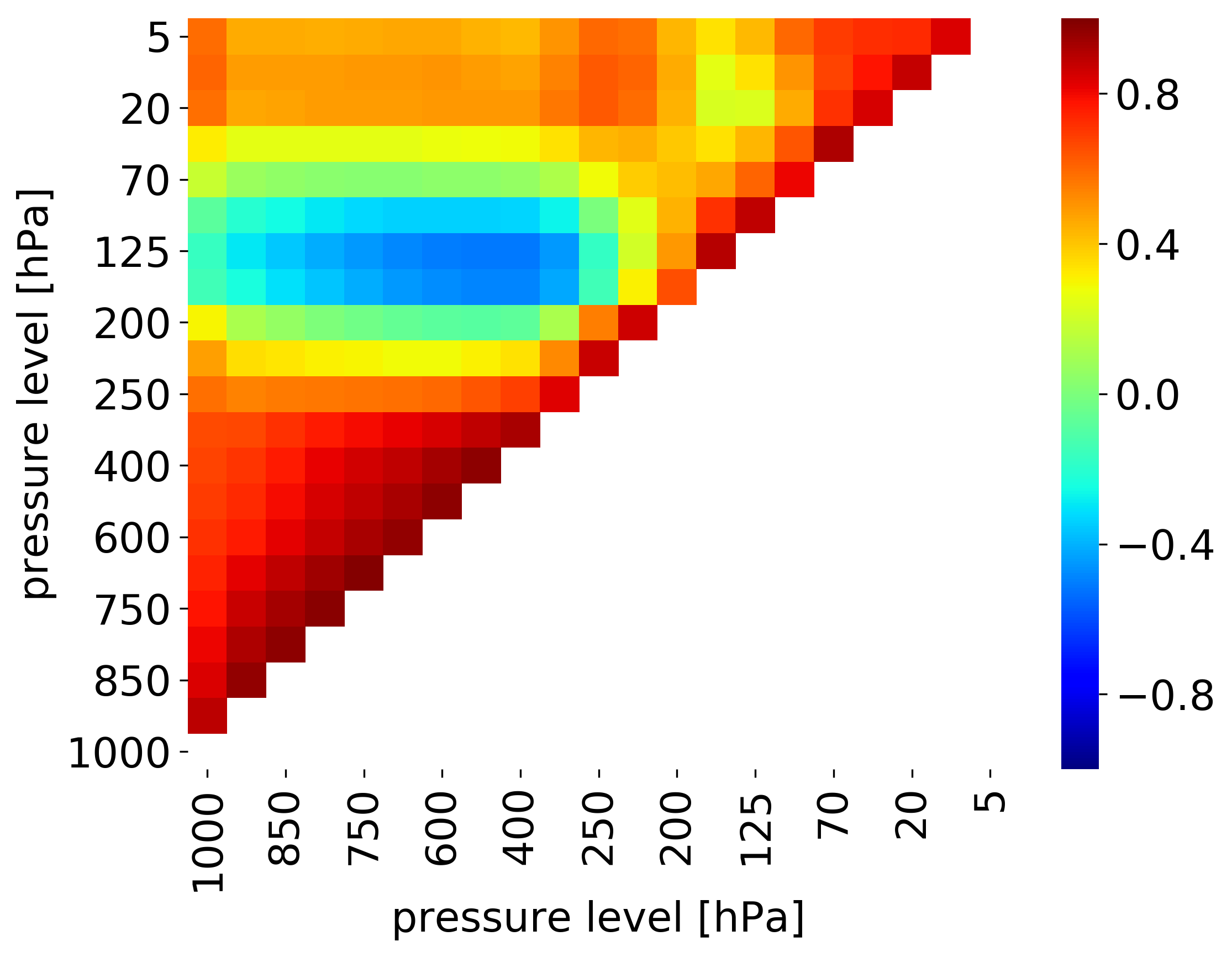
Figure 4: Pairwise correlations between daily temperature variations $\Delta T$ of the different pressure levels considered in this analysis for Santiago de Compostela (from January 2015 to December 2016).

An experimental determination of $W_{T}(h)$ is not straightforward, and requires special statistical techniques, given the presence of strong correlations between the temperature variations of the different atmospheric layers. Figure 4 shows the pairwise correlation matrix for the temperature variations of the different atmospheric layers on top of the detector. In general, the low stratosphere ($\sim$250-70 hPa) behaves opposite to the troposphere ($\sim$1000-250 hPa) and high stratosphere ($\sim$70-1 hPa). This is because the boundary layer ($\sim$925 hPa) is positively correlated with the rest of the troposphere through convection, while an increase in its temperature will generally result in the low stratosphere cooling down. This is a typical condition observed for latitude regions above 40^∘ [Liu . (2014)]. Consequently, any attempt to obtain the temperature coefficients by means of a multivariate regression will result in coefficients whose values do not correspond to the actual values. If explanatory variables of a multiple regression model are strongly correlated, they provide redundant information and violate the condition of non-colinearity required in a least-squares regression. The coefficients will also be highly sensitive to small changes in the model and their sign will be dramatically dependent on the variables considered. In other words, slightly different models might lead to different conclusions. In this way, we would never know the actual effect of each variable. Clearly, any phenomenological model aimed at reliably describing the measured rates needs to start from a sensible set of uncorrelated temperature variables, that need to be obtained beforehand. We adapt for the task the Principal Components Regression (PCR) analysis, that has been successfully used before for this type of studies in [Yanchukovsky  Kuzmenko (2018), Savić . (2019)].

4.1 Barometric Effect

Being much subtler, the temperature effect must be analyzed once the pressure effect has been removed. Moreover, in the case of gaseous detectors, the efficiency is a function of the ratio of electric field $E$ and pressure $P$ (represented by $E/P$ and dubbed reduced field), so even a high voltage and $T$-controlled environment is not sufficient to stabilize the detector response completely [Lopes . (2016)]. The above dependency means that the detector efficiency is anticorrelated with pressure, and will add to the barometric effect at ground. Considering the atmospheric effect first, the relative change in the secondary c.r. rate caused by variations of the ground-level pressure has an exponential dependence. To first order approximation, it can be expressed through a linear relation:

$$\frac{R}{R_{0}}=e^{\beta_{atm}\cdot\Delta P}\rightarrow\frac{\Delta R}{R_{0}}\Big{|}_{P}\approx\beta\cdot\Delta P$$ (1)

where $\frac{\Delta R}{R_{0}}\Big{|}_{P}$ is the relative variation of the c. r. rate due to the pressure effect, $R_{0}$ represents its average value over the period under consideration, $\Delta P=P-P_{0}$ is the deviation of the ground-level pressure with respect to its mean value ($P_{0}$) over the same period, and $\beta=\beta_{atm}+\beta_{det}$ is the barometric coefficient, with $\beta_{atm}$ representing the atmospheric effect and $\beta_{det}$ the detector contribution.

Figure 5: Example of the linear fit method used to obtain the barometric coefficient for one of the sub-periods. The green lines delimit the points left out of a 2-$\sigma$ interval after an iterative procedure. The blue line is the resulting regression line.

The barometric coefficient was obtained separately for five different sub-periods, that displayed slightly different stability conditions. An iterative linear fit was performed, with data outside a 2-$\sigma$ interval removed from the fit (Figure 5). Compatible barometric coefficients were obtained, whose mean value was determined to be $\beta=-0.59\pm 0.02$ %/hPa. This methodology allow us to remove any outliers in the data caused by detector instabilities and occasional space weather effects such as Forbush decreases or interplanetary events.

Finally, the barometric effect is removed using:

$$\frac{\Delta R}{R_{0}}\Big{|}_{T}=\frac{\Delta R}{R_{0}}\Big{|}_{obs}-\frac{\Delta R}{R_{0}}\Big{|}_{P}$$ (2)

where $\frac{\Delta R}{R_{0}}\Big{|}_{obs}$ are the experimental c.r. variations and $\frac{\Delta R}{R_{0}}\Big{|}_{T}$ the remaining variations due to the temperature effect.

4.2 Temperature effect

Variations of the measured rate of the secondary c.r. component due to the atmospheric temperature effect can be approximated by a linear combination of some temperature coefficients and the temperature variations of n atmospheric layers [Dmitrieva . (2011)]:

$$\frac{\Delta R}{R_{0}}\Big{|}_{T}=\sum_{i=1}^{n}W_{T}(h_{i})\Delta T_{i}\Delta h_{i}$$ (3)

where $\frac{\Delta R}{R_{0}}\Big{|}_{T}$ are the relative variations due to the temperature effect; $W_{T}$, given in % K^-1 atm^-1, is the corresponding temperature coefficient for the atmospheric layer i at pressure $h_{i}$; $\Delta T_{i}=T_{i}-T_{0_{i}}$ are the temperature variations within the same layer with respect to its mean value ($T_{0_{i}}$), and $\Delta h_{i}=h_{i-1}-h_{i}$ is the layer thickness, in atm.

Defining $k_{x_{i}}=W_{T}(h_{i})\Delta h_{i}$, equation 3 can be rewritten as

$$\frac{\Delta R}{R_{0}}\Big{|}_{T}=\sum_{i=1}^{n}k_{x_{i}}\Delta T_{i}$$ (4)

that we denote formally as

$$\mathbf{y}=\mathbf{X}\mathbf{k_{x}}$$ (5)

where y is the vector of the measured relative variations $\frac{\Delta R}{R_{0}}\Big{|}_{T}$; X is the ($m\times n$) data matrix of the temperature variations whose columns are the temperature variations of the $ith$ pressure level and $\mathbf{k_{x}}$ refers to the vector of temperature coefficients, that we want to estimate.

As mentioned earlier, the coefficients of this model can not be obtained by ordinary regression. For our purpose, we decided to use the Principal Component Regression (PCR) technique [Jolliffe (2002)]. This method is applied when a dataset of variables shows multicollinearity, in our case the temperature variations. The idea is to build new uncorrelated variables (called principal components), maintaining the information conveyed by the original ones, and use them as the new predictors to estimate the unkown regression coefficients of the model.

The PCA consists of an orthogonal linear transformation that converts the original variables to a new coordinate system. The principal components (PCs) represent the directions of the data containing the greatest variance. So, the first step is standardizing the $\Delta T_{i}$ measurements in X, dividing them by their standard deviations (over the analyzed period). This standardization is needed to prevent the variables with the highest variance from dominating. It causes a change in the notation, too. Too keep it simple, we mantain the current notation but taking into account that all the following calculations are based on standardized variables.

The principal components are the eigenvectors (directions) obtained from the covariance matrix of X and sorted by the amount of explained variance. This set of orthogonal vectors forms a new basis in the new coordinate system. The matrix X can be transformed using the matrix of eigenvectors, defined as A ($n\times n$), in the following way

$$\mathbf{P=XA}$$ (6)

where P is now the matrix ($m\times n$) containing the new variables in the new space. We got a set of uncorrelated variables because they were built using orthogonal eigenvectors. As a consequence, a new model can be built using variables P:

$$\mathbf{y=Pk_{p}}$$ (7)

Now, the new set of coefficients $\mathbf{k_{p}}$ can be obtained directly using a least-squares regression. Taking into account equation 6, we can write

$$\mathbf{y=XAk_{p}}$$ (8)

The regression coefficients $\mathbf{k_{p}}$ can be transformed back into the original space using equation 5 and 8

$$\mathbf{k_{x}=Ak_{p}}$$ (9)

and multiplying by standard deviations in order to go back to the original scale.

The year-to-year variability of the temperature data may affect the determination of the principal components, particularly if exceptional temperature changes took place during the data acquisition period, such as Stratospheric Warmings. This can be seen in Figures 6 and 7, where several stratospheric temperature anomalies (warmings and coolings) cab be seen during winter periods. Therefore, as a first step we use a training dataset from a time series of the last 30 years to determine the PCs of the temperature data and avoid the influence of outliers corresponding to exceptional events.

Figure 6: Temperature time series of the atmosphere in Santiago de Compostela from October 2015 to January 2017.

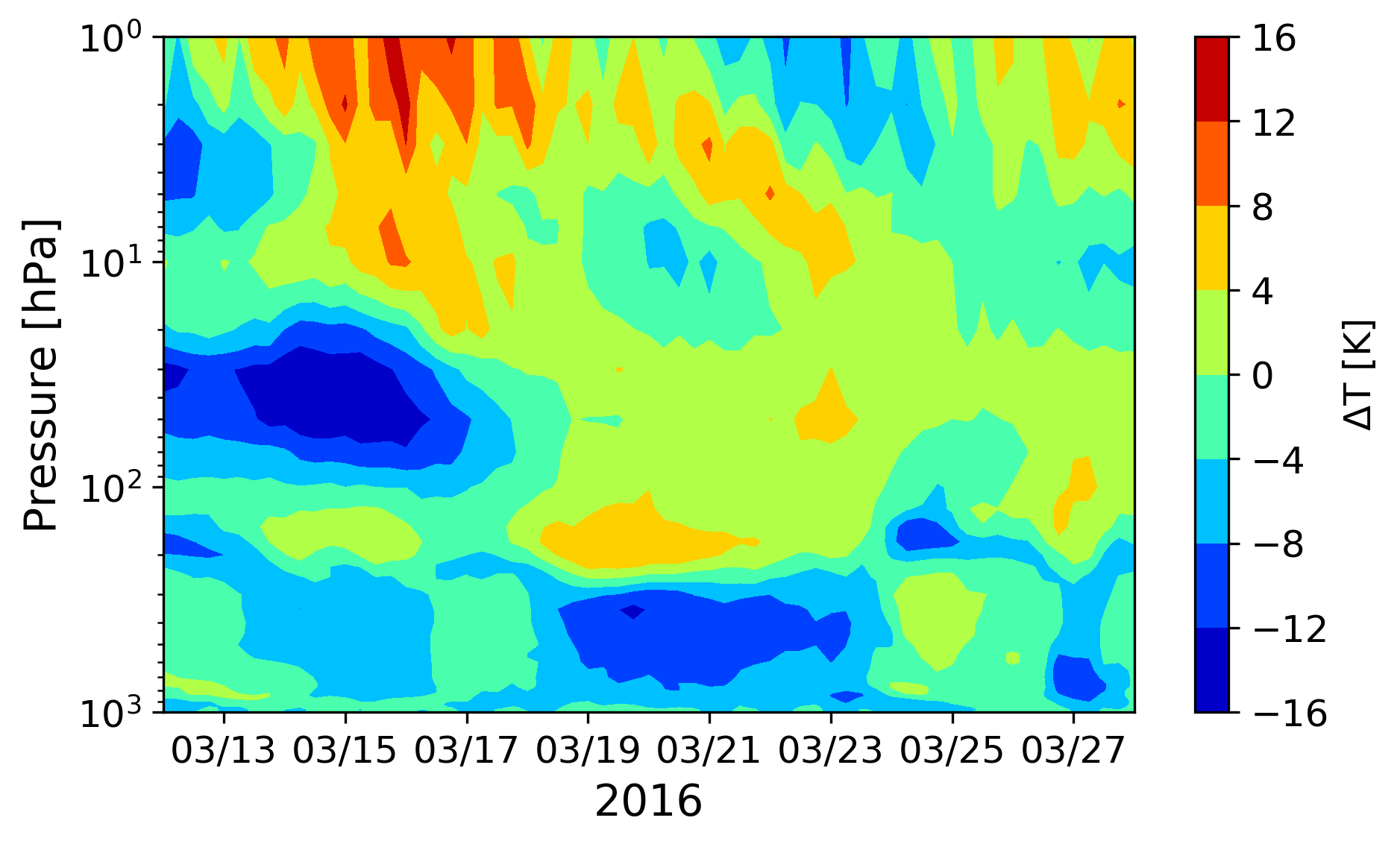
Figure 7: Temperature anomaly for March 2016 were an example of a Sudden Stratospheric Warming is observed in the first half of the month. The upper stratosphere warms rapidly in a few days propagating way down into the troposphere in the next weeks.

PCR typically uses only a significant subset of all the principal components P^′ to increase reliability. The components with higher variances are usually selected as the regressor variables for being the most important. No standard method exists for deciding how many components to retain. Anyhow, a good number of components should carry a high percentage of the total variance ($>$ 70%). In order to decide the number of PCs to keep, we previously performed an analysis with reconstructed cosmic ray variations using a theoretical distribution of the temperature coefficients as a proxy [Dmitrieva . (2011)]. These variations represent ideal data (i.e. without noise) only affected by the atmospheric temperature. Then, we apply the PCR method to these data to see how many PCs need to be kept in order to retrieve the original coefficients. To make this study more realistic, we follow the typical procedure of adding extra noise to the original data in three levels (low, medium and high) to be able to analyse the performance of the technique. It was observed that with two components it is possible to restore the correct values of the coefficients until an acceptable level of noise. Including more components destabilizes the result.

Finally, the vector of coefficients $\mathbf{k^{\prime}_{p}}$ is estimated by regressing the observed vector of cosmic ray data on the selected principal components $\mathbf{P^{\prime}}$ using least-squares regression. So equation 7 is reduced to

$$\mathbf{y=P^{\prime}k^{\prime}_{p}}$$ (10)

where $\mathbf{P^{\prime}}$ is now a matrix ($m\times r$) whose columns are the corresponding subset of columns of P (and $r<n$).

Using equation 9, $\mathbf{k^{\prime}_{p}}$ can be transformed back to the space of the actual temperature variables, providing the regression coefficients $\mathbf{k_{x}}$ that characterize the original model. Also, the relation $k_{x_{i}}=W_{T}(h_{i})\Delta h_{i}$ introduced before is taken into account when converting the estimated regression coefficients to the distribution of temperature coefficients $W_{T}$, having a dimension %/K$\cdot$atm.

It must be noted that Partial Least Squares (PLS) regression could be an alternative to this technique because it is similar to PCR in that both select components that explain the most variance in the model. The difference is that PLS incorporates the response variable (the c.r. rate, in this case) into the analysis. One of the main reasons for not using this method is that our set of cosmic rays measurements is limited to a period of just two years.

5 Results and Discussion

Figure 8a shows the distribution of temperature coefficients for the secondary c.r. component recorded at sea level for vertical incidence (blue line), where only events with a zenith angle $\theta$ lower than 13^∘ were selected. The PCR method was applied to five different sub-periods of the data in order to account for systematic effects, expected to be mostly of instrumental origin at this stage, but also any remaining space weather phenomena having similar timescales to temperature variations. The average value and error bars are obtained from this combined analysis.

Figure 8: (a) Distribution of temperature coefficients obtained with PCR for vertical tracks and comparison with the theoretical distribution for different energy thresholds: 0.15, 0.32, 0.75, 1 and 3.2 GeV. (b) Slopes $\tilde{W}_{T}$ obtained through a direct linear regression for the same data sample ($\theta<13^{\circ}$).

As mentioned, the detector is placed in the first floor of a two-floor building. Therefore, the composition of the overburden material has been taken into account to estimate the value of the threshold energy, $E_{th}\sim$ 0.15 GeV. The theoretical distributions for different energy thresholds and zenith angle $\theta=0^{\circ}$ (grey lines in Figure 8a) as given in [Dmitrieva . (2011)] are shown. A good agreement is observed for thresholds below 0.32 GeV, while above 0.75 GeV a systematic deviation appears, specially close to ground level.

Although being compatible, the estimated values in the troposphere ($>$300 hPa) are systematically above the theoretical ones. This might be a consequence of the method itself but could as well reflect the presence of the soft component in the measured rates, given that it anticipates a positive correlation with the lower layers of the atmosphere [Dorman (2004)]. The values also differ at high altitudes, in this case due to the constraint in the selection of the number of principal components in the analysis. The PCR method computes the principal components taking into account the variance in the temperature data. Then, the first components reproduce the general variations in the troposphere and stratosphere (seasonal changes). Variations in the high atmosphere are considerably more complex than in the surface, as illustrated in Figure 4. Increasing the selected number of components would help to reduce this effect in an ideal situation. However, the optimum number of selected components in our case is the one that allows to obtain the best results of the coefficients without the solution being destabilized by noise and other instrumental effects. On the other hand, it should be noted that the accuracy of the ECMWF reanalysis is worse at high altitudes (0-200 hPa) due to the lack of data (less satellite/balloon observations, etc), so the temperatures have an inherent source of error that surely increases the difficulties in obtaining the coefficients at those heights.

Figure 8b shows for illustration the slopes determined before applying the PCR. Each coefficient $\tilde{W}_{T}$ is obtained by direct regression between the relative variations of the c.r. intensity and the temperature variations for different layers:

$$\frac{\Delta R}{R_{0}}\Big{|}_{T}=\tilde{W}_{T}(h_{i})\Delta T_{i}\Delta h_{i}$$ (11)

These coefficients are dominated by the multiple correlations between the atmospheric layers. In particular, the slopes in the troposphere are negative, become positive in the low stratosphere and return to negative values in the high stratosphere. The distribution of temperature coefficients, $W_{T}(h)$, indicates that the contribution of the troposphere to the total rate variation is higher than the rest ($\sum_{i=1}^{trop}\Delta h_{i}/\sum_{i=1}^{n}\Delta h_{i}\sim 75\%$) and the values of the coefficients for this layer are negative. Therefore, when a direct regression is performed, the slopes $\tilde{W}_{T}$ in the troposphere will be negative with values close to the real ones, $W_{T}$. The observed slopes in the high stratosphere will be negative due to the positive correlation with the troposphere (Figure 4). And the slopes in the low stratosphere are slightly positive due to the anticorrelation with the troposphere. A comparison with Figure 8b illustrates that these correlations have been largely removed with the PCR method.

Once the distribution of temperature coefficients $W_{T}$ has been calculated, we can study the temperature effect. For this purpose, equation 3 can be used to build the so-called “effective temperature”, which allows to consider the entire atmospheric temperature profile through an unique parameter:

$$\frac{\Delta R}{R_{0}}\Big{|}_{T} = \sum_{i=1}^{n}W_{T}(h_{i})\Delta h_{i}\cdot\frac{\sum_{i=1}^{n}W_{T}(h_{i})\Delta T_{i}\Delta h_{i}}{\sum_{i=1}^{n}W_{T}(h_{i})\Delta h_{i}}=$$

$$= \alpha_{T}\Delta T_{eff}$$

Here the temperature coefficient $\alpha_{T}$ and the effective temperature $T_{eff}$ are defined as

$$\alpha_{T}=\sum_{i=1}^{n}W_{T}(h_{i})\Delta h_{i}$$ (13)

$$T_{eff}=\frac{\sum_{i=1}^{n}W_{T}(h_{i})T_{i}\Delta h_{i}}{\sum_{i=1}^{n}W_{T}(h_{i})\Delta h_{i}}$$ (14)

The definition of the effective temperature makes it possible to approximate the atmosphere as an isothermal body with a temperature $T_{eff}$, which is nothing but an average weighted by the product between the temperature coefficients and the atmospheric depth. It can be calculated using equation 14 with the corresponding temperature coefficients $W_{T}$. Moreover, the theoretical value $\alpha_{T_{theor}}=-0.319$ %/K is obtained using equation 13 for $E_{th}=0.15$ GeV. In our case, it can be experimentally calculated using the values of $W_{T}$ obtained by the PCR method:

$$\alpha_{T_{exp}}=-0.279\pm 0.051\;\mathrm{\%/K}$$

That is compatible with the theoretical one and also hints at the presence of the soft component, which could be the reason for the slight increase.

Table 1: Values of the temperature coefficients $\alpha_{T}$ and $\alpha_{MSS}$ obtained in this work, together with the deviation from independent estimates, dubbed $\Delta\alpha$.

	Theoretical [Dmitrieva . (2011)]	This work	$\Delta\alpha$
$\alpha_{T}$ (%/K)	-0.319	-0.279 $\pm$ 0.051	0.040 $\pm$ 0.051
	[Mendonça . (2019)]	This work	$\Delta\alpha$
$\alpha_{MSS}$ (%/K)	-0.271	-0.233 $\pm$ 0.045	0.038 $\pm$ 0.045

A complementary approach exists using the so-called mass-weighted temperature $T_{MSS}$ and its corresponding coefficient $\alpha_{MSS}$ [De Mendonça . (2016)]. In this case, the c.r. variations due to the temperature effect are approximated by

$$\frac{\Delta R}{R_{0}}\Big{|}_{T}=\alpha_{MSS}\Delta T_{MSS}$$ (15)

$$T_{MSS}=\sum_{i=1}^{n}T_{i}\cdot\left(\frac{x(h_{i})-x(h_{i+1})}{x(h_{0})}\right)$$ (16)

where $x(h_{i})$ is the atmospheric depth at the same altitude. Indeed, a very recent study from the GMDN [Mendonça . (2019)] found a relation between the mass-weighted temperature coefficient and the cutoff rigidity ($R_{c}$) and latitude ($L$) for vertical incidence:

$$\alpha_{MSS}=-0.304+0.0389\cdot\ln{R_{c}}-0.0488\cdot\sin{L}$$ (17)

Introducing in this equation the values for $R_{c}$ and $L$ corresponding to the location of our detector, we anticipate a temperature coefficient of -0.271 %/K. On the other hand, application of a linear regression to our data following equation 15 gives $\alpha_{MSS}=-0.233\pm 0.045$ %/K, which again points to contamination from the soft component. Our analysis is summarised in Table 1, highlighting the deviation from the other two estimates discussed in this work ($\Delta\alpha$). The fact that $\Delta\alpha$ is similar for both $\alpha_{MSS}$ and $\alpha_{T}$, suggests a common origin to the observed excess.

Figure 9 shows the secondary c.r. after pressure correction compared with the estimated temperature effect modeled through our two main PCs and their corresponding regression coefficients. The evolution of the effective temperature is shown as well. It is possible to appreciate the typical seasonal behavior reported by other detectors: c.r. rate reaches its maximum in winter when the atmosphere is colder while it declines towards summer when it is warmer. Moreover, the procedure is able to interpolate the temperature effect in those periods of missing data, such us July and August of 2016. Overall, the estimated temperature effect is able to reproduce $\sim 77$% of the variability of the observed data, demonstrating that the PCR is a reasonable method to recover the seasonal variability.

Figure 9: Top: cosmic ray rate corrected by pressure as observed by the TRAGALDABAS detector (red curve) and calculated via PCR method (black curve) compared with the effective temperature (blue curve). Bottom: zoom into the December 2016 Sudden Warming event, and P, $\Delta$T map on that period.

A significant behaviour is also observed at the end of 2016: rates show an abrupt decrease followed by a major increase (see zoom in Figure 9). The PCR method is able to reproduce this trend as well. If the temperature variations of this period are analysed, several cooling and warmings are observed: a Sudden Stratospheric Warming in the high stratosphere takes place, followed by a great cooling of at least -40 K. However, an opposite behaviour is observed in the low stratosphere.

The sign of the calculated distribution of the coefficients $W_{T}$ (Figure 8a) indicates that the negative temperature effect dominates throughout the atmosphere. This means that, if the temperature varies in any atmospheric layer, the measured rate will vary in inverse proportionallity to that indicated by the corresponding coefficient. Bearing this in mind, we can expect a measured rate decrease due to the increase of temperature in the troposphere and high stratosphere. However, the reduction of the temperature of the low stratosphere, given the presence of correlations between layers, will tend to increase the rates. The effective temperature describes the global effect of these different temperature variations. In this case, as the layers of the troposphere have more weight ($\sim$75% of the total atmospheric mass) with respect to the stratosphere, their effect is dominant and that is why the seasonal evolution of the effective temperature in Figure 9 is similar to the surface temperature, and appears anticorrelated with the observed rates.

The distribution of temperature coefficients can be used, along with the barometric coefficient, to remove the atmospheric effects and analyse space weather phenomena. This is briefly described in A with the analysis of a Forbush Decrease (FD) and will be the subject of future works.

To sum up, this is the first demonstration that the timing RPC technology can be succesfully applied to studies about the atmosphere condition, in particular its temperature profile. With the commissioning phase already over and the detector fully operative, additional work could focus on carrying out differential studies on the angular response as well as carefully correcting for space weather phenomena.

6 Conclusions

We have commissioned and calibrated a small-size 2 m² timing RPC detector devoted to the detailed study of cosmic rays at ground level, and performed the first analysis of the atmospheric temperature effect with this technology. By studying a data sample of barely one year, it has been possible to estimate the distribution of temperature coefficients ($W_{T}(h)$), showing that the contribution of the hard component is dominant and in good agreement with theoretical calculations.

We show how the presence of strong correlations among the different atmospheric layers precludes the use of conventional regression methods. A Principal Component Regression (PCR), considering the first two components, is sufficient to capture at least 77% of the variability, giving a good description of the $W_{T}(h)$ and the global slope parameter $\alpha_{T_{exp}}=-0.279\pm 0.051$ %/K (compared to a theoretical value of $\alpha_{T_{theor}}=-0.319$ %/K). This results in an anticorrelation with the effective atmospheric temperature, that allows to clearly identify its seasonal cycles as well as short-term exceptional events (such as the tropospheric consequences of a Sudden Stratospheric Warming), through measurements performed at ground level.

Appendix A Monitoring a Forbush Decrease

As mentioned in the introduction, c.r. measurements provide valuable data for different research areas, in particular space weather. But as we have seen so far, when analyzing variations in c.r. intensity using ground-based detectors, atmospheric effects cannot be ignored. The pressure and temperature effects produce significant variations. Therefore, it is important to remove those in order to study any solar or interplanetary phenomena [Dorman (2004)].

In June 2015 the Sun was very active and produced a significant number of coronal mass ejections towards the Earth, initiating a large Forbush Decrease (FD) event (more information at [The SOHO/LASCO CME Catalog ()]). A FD may be caused when a solar disturbance travels away from the Sun towards the Earth, affecting the galactic cosmic ray flux, which conveys the most energetic particles coming from outside the heliosphere. Such disturbance will produce a region of suppressed c.r. density located downstream of the coronal mass ejection, behind the interplanetary shock which this fast ejection produces in the medium ahead of it. In such a case, the c.r. intensity at ground shows a fast decrease, reaching a minimum within about a day, followed by a slow recovery phase lasting for several days [Cane (2000)].

The decrease in the TRAGALDABAS counting rate on 22 June 2015 is the first FD registered over the period from 2015 to 2017. Figure 10 shows the relative variations before corrections (grey), corrected only by pressure (blue) and corrected by both temperature and pressure (red) in the period from 18 June to 6 July, 2015. A fast decreasing phase is observed after pressure corrections, reaching a minimum in a couple of days of about $\sim$4%, and followed by a slow recovery phase during the next days. Without atmospheric corrections, this characteristic FD behaviour is not discernible.

Figure 10: Forbush Decrease event on 22 June 2015: uncorrected (grey curve), only pressure corrected (blue curve) and pressure and temperature corrected variations (red curve).

References

- Abbrescia \BOthers. (\APACyear2013) \APACinsertmetastarEEE{APACrefauthors}Abbrescia, M., Agocs, A., Aiola, S., Antolini, R., Avanzini, C., Ferroli, R\BPBIB.\BDBLothers \APACrefYearMonthDay2013. \BBOQ\APACrefatitleThe EEE experiment project: status and first physics results The EEE experiment project: status and first physics results.\BBCQ \APACjournalVolNumPagesThe European Physical Journal Plus128662. \PrintBackRefs\CurrentBib
- Abrahao \BOthers. (\APACyear2017) \APACinsertmetastardoublechooz{APACrefauthors}Abrahao, T., Almazan, H., Dos Anjos, J., Appel, S., Baussan, E., Bekman, I.\BDBLothers \APACrefYearMonthDay2017. \BBOQ\APACrefatitleCosmic-muon characterization and annual modulation measurement with Double Chooz detectors Cosmic-muon characterization and annual modulation measurement with double chooz detectors.\BBCQ \APACjournalVolNumPagesJournal of Cosmology and Astroparticle Physics201702017. \PrintBackRefs\CurrentBib
- Abreu \BOthers. (\APACyear2018) \APACinsertmetastarLuisMarta{APACrefauthors}Abreu, P., Andringa, S., Assis, P., Blanco, A.\BCBL \BOthersPeriod. \APACrefYearMonthDay2018. \BBOQ\APACrefatitleMARTA: a high-energy cosmic-ray detector concept for high-accuracy muon measurement MARTA: a high-energy cosmic-ray detector concept for high-accuracy muon measurement.\BBCQ \APACjournalVolNumPagesThe European Physics Journal C783331-11. \PrintBackRefs\CurrentBib
- An \BOthers. (\APACyear2008) \APACinsertmetastarWilliams24{APACrefauthors}An, S., Jo, Y\BPBIK., S, K\BPBIJ., M, K\BPBIM., D, H., S, W\BPBIM\BPBIC.\BDBLR, Z. \APACrefYearMonthDay2008. \BBOQ\APACrefatitleA 20ps timing device —A Multigap Resistive Plate Chamber with 24 gas gaps A 20ps timing device —A Multigap Resistive Plate Chamber with 24 gas gaps.\BBCQ \APACjournalVolNumPagesNucl. Instr. Meth. A59439-43. \PrintBackRefs\CurrentBib
- Belver \BOthers. (\APACyear2010) \APACinsertmetastarDANIFEE{APACrefauthors}Belver, D., Cabanelas, P., Castro, E., Garzon, J\BPBIA., Gil, A., Gonzalez-Diaz, D.\BDBLTraxler, M. \APACrefYearMonthDay2010. \BBOQ\APACrefatitlePerformance of the low-jitter high-gain/bandwidth front-end electronics of the HADES tRPC wall Performance of the low-jitter high-gain/bandwidth front-end electronics of the HADES tRPC wall.\BBCQ \APACjournalVolNumPagesIEEE Trans. Nucl. Sci.572848-2856. {APACrefDOI} 10.1109/TNS.2010.2056928 \PrintBackRefs\CurrentBib
- Berkova \BOthers. (\APACyear2011) \APACinsertmetastarberkova{APACrefauthors}Berkova, M., Belov, A., Eroshenko, E.\BCBL \BBA Yanke, V. \APACrefYearMonthDay2011. \BBOQ\APACrefatitleTemperature effect of the muon component and practical questions for considering it in real time Temperature effect of the muon component and practical questions for considering it in real time.\BBCQ \APACjournalVolNumPagesBulletin of the Russian Academy of Sciences: Physics756820–824. {APACrefDOI} 10.3103/s1062873811060086 \PrintBackRefs\CurrentBib
- Blackett (\APACyear1938) \APACinsertmetastarblackett{APACrefauthors}Blackett, P\BPBIM. \APACrefYearMonthDay1938. \BBOQ\APACrefatitleOn the instability of the barytron and the temperature effect of cosmic rays On the instability of the barytron and the temperature effect of cosmic rays.\BBCQ \APACjournalVolNumPagesPhysical Review5411973. {APACrefDOI} 10.1103/physrev.54.973 \PrintBackRefs\CurrentBib
- Blanco \BOthers. (\APACyear2015) \APACinsertmetastarneutrons2{APACrefauthors}Blanco, A., Adamczewski-Musch, J., Boretzky, K., Cabanelas, P., Cartegni, L., Marques, R\BPBIF.\BDBLothers \APACrefYearMonthDay2015. \BBOQ\APACrefatitlePerformance of timing resistive plate chambers with relativistic neutrons from 300 to 1500 MeV Performance of timing resistive plate chambers with relativistic neutrons from 300 to 1500 mev.\BBCQ \APACjournalVolNumPagesJournal of Instrumentation1002C02034. \PrintBackRefs\CurrentBib
- Blanco \BOthers. (\APACyear2014) \APACinsertmetastartragaldabas{APACrefauthors}Blanco, A., Blanco, J., Collazo, J., Fonte, P., Garzón, J., Gómez, A.\BDBLothers \APACrefYearMonthDay2014. \BBOQ\APACrefatitleTRAGALDABAS: a new RPC based detector for the regular study of cosmic rays Tragaldabas: a new rpc based detector for the regular study of cosmic rays.\BBCQ \APACjournalVolNumPagesJournal of Instrumentation909C09027. {APACrefDOI} 10.1088/1748-0221/9/09/c09027 \PrintBackRefs\CurrentBib
- Cane (\APACyear2000) \APACinsertmetastarforbush{APACrefauthors}Cane, H\BPBIV. \APACrefYearMonthDay2000. \BBOQ\APACrefatitleCoronal mass ejections and Forbush decreases Coronal mass ejections and forbush decreases.\BBCQ \BIn \APACrefbtitleCosmic Rays and Earth Cosmic rays and earth (\BPGS 55–77). \APACaddressPublisherSpringer. \PrintBackRefs\CurrentBib
- Cerrón Zeballos \BOthers. (\APACyear1996) \APACinsertmetastarMultigap{APACrefauthors}Cerrón Zeballos, E., Crotty, I., Hatzifotiadou, D., Lamas Valverde, J., Neupane, S., Williams, M\BPBIC\BPBIS.\BCBL \BBA Zichichi, A. \APACrefYearMonthDay1996. \BBOQ\APACrefatitleA new type of resistive plate chamber: The multigap RPC A new type of resistive plate chamber: The multigap RPC.\BBCQ \APACjournalVolNumPagesNucl. Instr. Meth. A374132-135. \PrintBackRefs\CurrentBib
- Dee \BOthers. (\APACyear2011) \APACinsertmetastarerainterim{APACrefauthors}Dee, D\BPBIP., Uppala, S., Simmons, A., Berrisford, P., Poli, P., Kobayashi, S.\BDBLothers \APACrefYearMonthDay2011. \BBOQ\APACrefatitleThe ERA-Interim reanalysis: Configuration and performance of the data assimilation system The era-interim reanalysis: Configuration and performance of the data assimilation system.\BBCQ \APACjournalVolNumPagesQuarterly Journal of the royal meteorological society137656553–597. {APACrefDOI} 10.1002/qj.828 \PrintBackRefs\CurrentBib
- De Mendonça \BOthers. (\APACyear2016) \APACinsertmetastarmendonca{APACrefauthors}De Mendonça, R., Braga, C., Echer, E., Dal Lago, A., Munakata, K., Kuwabara, T.\BDBLothers \APACrefYearMonthDay2016. \BBOQ\APACrefatitleThe temperature effect in secondary cosmic rays (muons) observed at the ground: analysis of the Global MUON Detector Network data The temperature effect in secondary cosmic rays (muons) observed at the ground: analysis of the global muon detector network data.\BBCQ \APACjournalVolNumPagesThe Astrophysical Journal830288. {APACrefDOI} 10.3847/0004-637x/830/2/88 \PrintBackRefs\CurrentBib
- De Mendonca \BOthers. (\APACyear2013) \APACinsertmetastarmendonca_simple{APACrefauthors}De Mendonca, R., Raulin, J\BHBIP., Echer, E., Makhmutov, V.\BCBL \BBA Fernandez, G. \APACrefYearMonthDay2013. \BBOQ\APACrefatitleAnalysis of atmospheric pressure and temperature effects on cosmic ray measurements Analysis of atmospheric pressure and temperature effects on cosmic ray measurements.\BBCQ \APACjournalVolNumPagesJournal of Geophysical Research: Space Physics11841403–1409. {APACrefDOI} 10.1029/2012ja018026 \PrintBackRefs\CurrentBib
- Dmitrieva \BOthers. (\APACyear2013) \APACinsertmetastardmitrievamethods{APACrefauthors}Dmitrieva, A., Astapov, I., Kovylyaeva, A.\BCBL \BBA Pankova, D. \APACrefYearMonthDay2013. \BBOQ\APACrefatitleTemperature effect correction for muon flux at the Earth surface: estimation of the accuracy of different methods Temperature effect correction for muon flux at the earth surface: estimation of the accuracy of different methods.\BBCQ \BIn \APACrefbtitleJournal of Physics: Conference Series Journal of physics: Conference series (\BVOL 409, \BPG 012130). {APACrefDOI} 10.1088/1742-6596/409/1/012130 \PrintBackRefs\CurrentBib
- Dmitrieva \BOthers. (\APACyear2011) \APACinsertmetastardmitrievacoef{APACrefauthors}Dmitrieva, A., Kokoulin, R., Petrukhin, A.\BCBL \BBA Timashkov, D. \APACrefYearMonthDay2011. \BBOQ\APACrefatitleCorrections for temperature effect for ground-based muon hodoscopes Corrections for temperature effect for ground-based muon hodoscopes.\BBCQ \APACjournalVolNumPagesAstroparticle Physics346401–411. {APACrefDOI} 10.1016/j.astropartphys.2010.10.013 \PrintBackRefs\CurrentBib
- Dorman (\APACyear2004) \APACinsertmetastardorman{APACrefauthors}Dorman, L. \APACrefYear2004. \APACrefbtitleCosmic Rays in the Earth Atmosphere and Underground Cosmic rays in the earth atmosphere and underground. \APACaddressPublisherSpringer Science & Business Media. \PrintBackRefs\CurrentBib
- Duperier (\APACyear1949) \APACinsertmetastarduperier{APACrefauthors}Duperier, A. \APACrefYearMonthDay1949. \BBOQ\APACrefatitleThe Meson Intensity at the Surface of the Earth and the Temperature at the Production Level The meson intensity at the surface of the earth and the temperature at the production level.\BBCQ \APACjournalVolNumPagesProceedings of the Physics Society. Section A6211684. {APACrefDOI} 10.1088/0370-1298/62/11/302 \PrintBackRefs\CurrentBib
- Fonte \BOthers. (\APACyear2000) \APACinsertmetastaralice{APACrefauthors}Fonte, P., Smirnitski, A.\BCBL \BBA Williams, M. \APACrefYearMonthDay2000. \BBOQ\APACrefatitleA new high-resolution TOF technology A new high-resolution tof technology.\BBCQ \APACjournalVolNumPagesNuclear Instruments and Methods in Physics Research Section A: Accelerators, Spectrometers, Detectors and Associated Equipment4431201–204. \PrintBackRefs\CurrentBib
- Hayashi \BOthers. (\APACyear2005) \APACinsertmetastargrapes{APACrefauthors}Hayashi, Y., Aikawa, Y., Gopalakrishnan, N., Gupta, S., Ikeda, N., Ito, N.\BDBLothers \APACrefYearMonthDay2005. \BBOQ\APACrefatitleA large area muon tracking detector for ultra-high energy cosmic ray astrophysics—the GRAPES-3 experiment A large area muon tracking detector for ultra-high energy cosmic ray astrophysics—the GRAPES-3 experiment.\BBCQ \APACjournalVolNumPagesNuclear Instruments and Methods in Physics Research Section A: Accelerators, Spectrometers, Detectors and Associated Equipment5453643–657. {APACrefDOI} 10.1016/j.nima.2005.02.020 \PrintBackRefs\CurrentBib
- Hippler \BOthers. (\APACyear2008) \APACinsertmetastarmustang{APACrefauthors}Hippler, R., Mengel, A., Jansen, F., Bartling, G., Göhler, W., Kudela, K.\BDBLothers \APACrefYearMonthDay2008. \BBOQ\APACrefatitleFirst space weather observations at MuSTAnG–the muon space weather telescope for anisotropies at Greifswald First space weather observations at mustang–the muon space weather telescope for anisotropies at greifswald.\BBCQ \BIn \APACrefbtitleProc. of 30th International Cosmic Ray Conference, Mexico Proc. of 30th international cosmic ray conference, mexico (\BVOL 1, \BPGS 347–350). \PrintBackRefs\CurrentBib
- Hubert \BOthers. (\APACyear2016) \APACinsertmetastarneutrons3{APACrefauthors}Hubert, G., Pazianotto, M.\BCBL \BBA Federico, C. \APACrefYearMonthDay2016. \BBOQ\APACrefatitleModeling of ground albedo neutrons to investigate seasonal cosmic ray-induced neutron variations measured at high-altitude stations Modeling of ground albedo neutrons to investigate seasonal cosmic ray-induced neutron variations measured at high-altitude stations.\BBCQ \APACjournalVolNumPagesJournal of Geophysical Research: Space Physics1211212–186. \PrintBackRefs\CurrentBib
- Jolliffe (\APACyear2002) \APACinsertmetastarpca_book{APACrefauthors}Jolliffe, I\BPBIT. \APACrefYearMonthDay2002. \BBOQ\APACrefatitlePrincipal components in regression analysis Principal components in regression analysis.\BBCQ \APACjournalVolNumPagesPrincipal component analysis168–177. \PrintBackRefs\CurrentBib
- Kornakov (\APACyear2014) \APACinsertmetastarKorna{APACrefauthors}Kornakov, G. \APACrefYearMonthDay2014. \BBOQ\APACrefatitleTime of flight measurement in heavy-ion collisions with the HADES RPC TOF wall Time of flight measurement in heavy-ion collisions with the HADES RPC TOF wall.\BBCQ \APACjournalVolNumPagesJINST 9 (2014) no.11, C11015911. \PrintBackRefs\CurrentBib
- Liu \BOthers. (\APACyear2014) \APACinsertmetastartropopause{APACrefauthors}Liu, Y., Xu, T.\BCBL \BBA Liu, J. \APACrefYearMonthDay2014. \BBOQ\APACrefatitleCharacteristics of the seasonal variation of the global tropopause revealed by COSMIC/GPS data Characteristics of the seasonal variation of the global tropopause revealed by cosmic/gps data.\BBCQ \APACjournalVolNumPagesAdvances in Space Research54112274–2285. {APACrefDOI} 10.1016/j.asr.2014.08.020 \PrintBackRefs\CurrentBib
- Lopes \BOthers. (\APACyear2016) \APACinsertmetastarRPC{APACrefauthors}Lopes, L., Assis, P., Blanco, A., Carolino, N., Cerda, M., Conceição, R.\BDBLothers \APACrefYearMonthDay2016. \BBOQ\APACrefatitleOutdoor field experience with autonomous RPC based stations Outdoor field experience with autonomous RPC based stations.\BBCQ \APACjournalVolNumPagesJournal of Instrumentation1109C09011. {APACrefDOI} 10.1088/1748-0221/11/09/c09011 \PrintBackRefs\CurrentBib
- Margato \BOthers. (\APACyear2019) \APACinsertmetastarneutrons1{APACrefauthors}Margato, L., Morozov, A., Blanco, A., Fonte, P., Fraga, F., Guerard, B.\BDBLothers \APACrefYearMonthDay2019. \BBOQ\APACrefatitleBoron-10 lined RPCs for sub-millimeter resolution thermal neutron detectors: Feasibility study in a thermal neutron beam Boron-10 lined RPCs for sub-millimeter resolution thermal neutron detectors: Feasibility study in a thermal neutron beam.\BBCQ \APACjournalVolNumPagesJournal of Instrumentation1401P01017. \PrintBackRefs\CurrentBib
- Mendonça \BOthers. (\APACyear2019) \APACinsertmetastarmendonca_rigidity{APACrefauthors}Mendonça, R., Wang, C., Braga, C., Echer, E., Dal Lago, A., Costa, J.\BDBLothers \APACrefYearMonthDay2019. \BBOQ\APACrefatitleAnalysis of cosmic rays’ atmospheric effects and their relationships to cutoff rigidity and zenith angle using Global Muon Detector Network data Analysis of cosmic rays’ atmospheric effects and their relationships to cutoff rigidity and zenith angle using global muon detector network data.\BBCQ \APACjournalVolNumPagesJournal of Geophysical Research: Space Physics. \PrintBackRefs\CurrentBib
- Pierre Auger Collaboration (\APACyear2015) \APACinsertmetastarpierre{APACrefauthors}Pierre Auger Collaboration, C. \APACrefYearMonthDay2015. \BBOQ\APACrefatitleThe Pierre Auger cosmic ray observatory The pierre auger cosmic ray observatory.\BBCQ \APACjournalVolNumPagesNuclear Instruments and Methods in Physics Research Section A: Accelerators, Spectrometers, Detectors and Associated Equipment798172–213. {APACrefDOI} 10.1016/j.nima.2015.06.058 \PrintBackRefs\CurrentBib
- Rockenbach \BOthers. (\APACyear2014) \APACinsertmetastarGMDN{APACrefauthors}Rockenbach, M., Dal Lago, A., Schuch, N., Munakata, K., Kuwabara, T., Oliveira, A.\BDBLothers \APACrefYearMonthDay2014. \BBOQ\APACrefatitleGlobal muon detector network used for space weather applications Global muon detector network used for space weather applications.\BBCQ \APACjournalVolNumPagesSpace Science Reviews1821-41–18. {APACrefDOI} 10.1007/s11214-014-0048-4 \PrintBackRefs\CurrentBib
- Sagisaka (\APACyear1986) \APACinsertmetastarsagisaka{APACrefauthors}Sagisaka, S. \APACrefYearMonthDay1986. \BBOQ\APACrefatitleAtmospheric effects on cosmic-ray muon intensities at deep underground depths Atmospheric effects on cosmic-ray muon intensities at deep underground depths.\BBCQ \APACjournalVolNumPagesIl Nuovo Cimento C94809–828. {APACrefDOI} 10.1007/bf02558081 \PrintBackRefs\CurrentBib
- Savić \BOthers. (\APACyear2019) \APACinsertmetastarpca2019{APACrefauthors}Savić, M., Dragić, A., Maletić, D., Veselinović, N., Banjanac, R., Joković, D.\BCBL \BBA Udovičić, V. \APACrefYearMonthDay2019. \BBOQ\APACrefatitleA novel method for atmospheric correction of cosmic-ray data based on principal component analysis A novel method for atmospheric correction of cosmic-ray data based on principal component analysis.\BBCQ \APACjournalVolNumPagesAstroparticle Physics1091–11. {APACrefDOI} 10.1016/j.astropartphys.2019.01.006 \PrintBackRefs\CurrentBib
- \APACcitebtitleThe SOHO/LASCO CME Catalog (\APACyear\bibnodate) \APACinsertmetastarsoho_nasa\APACrefbtitleThe SOHO/LASCO CME Catalog. The soho/lasco cme catalog. \APACrefYearMonthDay\bibnodate. {APACrefURL} https://cdaw.gsfc.nasa.gov/CME_list/UNIVERSAL/2015_06/univ2015_06.html \PrintBackRefs\CurrentBib
- Watanabe \BOthers. (\APACyear2019) \APACinsertmetastarWatanabe{APACrefauthors}Watanabe, K., Tanaka, S., Chang, W\BPBIC., Chen, H., Chu, M\BPBIL., Cuenca-García, J\BPBIJ.\BDBLYosoi, M. \APACrefYearMonthDay2019. \BBOQ\APACrefatitleA compensated multi-gap RPC with 2m strips for the LEPS2 experiment A compensated multi-gap RPC with 2m strips for the LEPS2 experiment.\BBCQ \APACjournalVolNumPagesNucl. Instr. Meth. A9251188-192. \PrintBackRefs\CurrentBib
- Yanchukovsky \BBA Kuzmenko (\APACyear2018) \APACinsertmetastaryanchuk_pca{APACrefauthors}Yanchukovsky, V.\BCBT \BBA Kuzmenko, V. \APACrefYearMonthDay2018. \BBOQ\APACrefatitleAtmospheric effects of the cosmic-ray mu-meson component Atmospheric effects of the cosmic-ray mu-meson component.\BBCQ \APACjournalVolNumPagesSolar-Terrestrial Physics4376–82. {APACrefDOI} 10.12737/stp-43201810 \PrintBackRefs\CurrentBib