Supplementary Information
Scaling of contact networks for epidemic spreading in urban transit systems
S1 Data
S1.1 Metro Trip data
The metro smart card transaction data are from three major cities in China: Shanghai, Guangzhou, and Shenzhen. These data have similar structure, with each record containing the information of smart card ID, transaction ID, transaction time, boarding station/time, and alighting station/time. The transaction type indicates if the transaction is entry or exit at the transaction station. Since each smart card is associated with a unique ID, we can therefore construct the trip sequences for each commuter (each card) based on the transaction time, transaction type and the location. We present a sample of smart card transaction data of Shenzhen on April 21st, 2016 in Tab S1.
| User ID | Transaction Type | Time | Station ID |
|---|---|---|---|
| 80357781 | 22 | 08:39:50 | 1 |
| 290452424 | 22 | 08:39:32 | 1 |
| 20353676 | 22 | 09:41:43 | 1 |
| 361341888 | 21 | 07:15:36 | 1 |
| 329838057 | 22 | 07:47:08 | 1 |
| 667519928 | 22 | 08:34:07 | 1 |
| 329213920 | 21 | 07:37:19 | 1 |
For each city, we extract the data of five work days for further analysis. A summary statistics of the data and the size of the metro networks that corresponded to the period of available data is shown in Table S2. When compared with official statistics of daily ridership, we observe that the smart card transaction data may cover over 60% of total daily travelers and can well reflect the trip dynamics of regular metro users. The metro networks in these cities have distinct layouts which are tailored to the urban form. Shanghai metro is the metro system with the longest total mileage and largest number of stations. It also has the highest number of daily travelers. Guangzhou and Shenzhen are similar in terms of the size of the metro networks, however, the shape of the metro network differs. In particular, Shenzhen is a stripe-shape city where commercial areas are located in the middle and residential places are distributed at east and west sides of the city. The layouts of metro networks and half-hourly passenger demand distributions of the three cities are presented in Figure S1. Note that the layouts presented here correspond to the period of time when the data were collected.


| City | Start date | End date | # metro lines | # stations | Average daily records |
|---|---|---|---|---|---|
| Guangzhou | 2017.04.13 | 2017.04.17 | 8 | 166 | 1.6 million |
| Shanghai | 2015.04.13 | 2015.04.17 | 13 | 288 | 4.16 million |
| Shenzhen | 2016.04.14 | 2016.04.18 | 5 | 118 | 2.13 million |
S1.2 Operation data
In order to infer the contact among travelers, we also need operation data which include the trip time between two adjacent metro stations, the approximate transfer time at transfer stations, and the frequency of metro trains.
To obtain these data, we developed web crawlers and extracted the metro station adjacency matrix from GaoDe Map API gaodemap as the representation of the metro system layouts . In addition, the time tables of the three metro systems were obtained from their official websites guangzhou_timetable ; shanghai_timetable ; shenzhen_timetable , which contain the travel time between two stations as well as the frequency of the metro trains during different time periods. Finally, the transfer time required between at the transfer station is calculated by identifying a route that needs a transfer at the station, quoting the travel time of the route using GaoDe Map API and subtracting the travel time of the route based on the values that we obtained from the timetable.
S2 Metro Contact Network
S2.1 Unweighted metro contact network
Based on the smart card transaction data and operation data for metro networks, we next develop the algorithm for constructing metro contact network (MCN). The contact network is constructed at individual level and we consider both unweighted and weighted contact networks. For unweighted MCN, each node represents a traveler and the link between a pair of nodes denotes that the two travelers will have positive probability to be on the same metro train. Since the smart card data only contain the time and location of a traveler entering and leaving the metro system, we need to infer if two travelers will be on the same metro train based on their trip starting time, origin station and destination station. And this further requires us to predict their travel route within the metro system. While the operation timetable of metro system is largely reliable, we assume that all travelers will follow the shortest route between two trip origin and destination (including both station-wise travel time and transfer time). Based on the predicted travel route, we can therefore determine if an link exists between two travelers following
-
1.
Find the shortest travel route for each traveler.
-
2.
For each pair of passenger and , determine if they have overlapping travel segments .
-
3.
If , determine their first meeting location, station , and calculate their arrival time at the meeting station respectively.
-
4.
Compute the probability of contact between travelers and based on and the frequency of metro lines.
-
5.
Repeat this process until all pairs of travelers are processed. Output .
In step 1, the shortest route can be computed using the Dijkstra algorithm with the travel time adjacency matrix , and the shortest routes are stored as sequences of the stations along the routes. In step 2 and 3, the overlapping travel segments of two travelers and can be identified as the longest common subsequence (LCS) of their routes and . In our case, a valid LCS that may grant contact is the LCS of length 2 or higher, indicating that the two travelers share at least one trip segment. In step 4, can be computed from their departure time and the trip time between their origin station and first meeting station . Then their contact probability follows
| (1) |
This suggests that two travelers will have positive contact probability if the gap between their arrival time at is less than the frequency of metro trains. And this probability decreases linearly considering the uniform arrival of metro trains following frequency .
S2.2 Weighted metro contact network
Based on unweighted MCNs, we further assign the weight to each link in unweighted MCNs to produce weighted MCNs. In the context of modeling the spread of communicable diseases, the weight on each link has the physical meaning as the expected contact duration between two individuals within effective transmission range. By effective transmission range, we consider that two individuals are close enough so that the airborne transmission of an communicable disease is feasible. This follows from the definition of the effective range for droplet transmission, which is usually less than 3 feet while certain disease such as SARS may reach 6 feet siegel20072007 . Let denote the scaling parameter for the effective transmission range, we have the weight between traveler and as:
| (2) |
Considering that a metro train consists of 6 coaches, with each coach of length 72 feet, then C may take the value of 144 if the effective transmission range is 3 feet. And equation 2 characterizes the expected contact duration as the product of the probability for being in effective transmission range and the duration of the contact , with the underlying assumption that travelers will uniformly distribute themselves among all metro coaches. The use of naturally captures the behavior of travelers to avoid congested coaches during travel. With increasing number of travelers (e.g. more number of nodes in MCNs), this also characterizes the linearly increasing chance of close contacts, where the total contact duration of each individual is the row sum of the contact duration matrix.
Finally, for the transmission rate of communicable disease, let denote the transmission strength per unit time, we have the transmission rate between two travelers as:
| (3) |
With the above processes, we can use the smart card data to generate sample unweigted and weighted MCNs. Specifically, the smart card data can be aggregated to generate the distributions for trip origin and destinations and the arrival time at each station. We then sample travelers following the distributions, where each traveler has their time of arrival, the origin station and the destination station. And the MCNs with nodes can consequently be constructed following the generation process for MCNs. We denote as the adjacency matrix of the generated MCNs, with each entry .
S2.3 Structural property of MCNs
| Number of nodes | Average path length | Average clustering coefficient | Assortativity | Diameter | <k> | <> | <> | <d> | <> | <> |
|---|---|---|---|---|---|---|---|---|---|---|
| 500 | 2.99 | 0.48 | 0.27 | 6.90 | 18.00 | 416.37 | 45.10 | 7.97 | 102.52 | 30.74 |
| 1000 | 2.79 | 0.49 | 0.26 | 7.20 | 35.09 | 1,562.10 | 89.50 | 15.95 | 401.66 | 59.99 |
| 1500 | 2.68 | 0.49 | 0.24 | 6.80 | 53.64 | 3,610.10 | 126.70 | 23.68 | 873.08 | 89.61 |
| 2000 | 2.64 | 0.49 | 0.25 | 7.10 | 71.03 | 6,322.30 | 169.70 | 31.83 | 1,564.80 | 117.92 |
| 2500 | 2.60 | 0.49 | 0.25 | 6.30 | 89.55 | 10,027 | 209.70 | 40.22 | 2,503.40 | 148.33 |
| 3000 | 2.58 | 0.49 | 0.25 | 6.40 | 106.15 | 14,085 | 247.20 | 47.35 | 3,434.80 | 173.65 |
| 3500 | 2.55 | 0.49 | 0.25 | 6.60 | 124.88 | 19,444 | 292.20 | 56.30 | 4,862.50 | 208.17 |
| 4000 | 2.54 | 0.49 | 0.24 | 6.40 | 141.92 | 25,075 | 337.50 | 63.51 | 6,168.50 | 237.69 |
| 4500 | 2.52 | 0.49 | 0.26 | 5.90 | 160.94 | 32,346 | 378.70 | 72.05 | 7,966.40 | 259.52 |
| 5000 | 2.51 | 0.49 | 0.24 | 6.40 | 177.68 | 39,327 | 411.20 | 79.09 | 9,583.30 | 292.39 |
| 5500 | 2.50 | 0.49 | 0.25 | 6.20 | 197.53 | 48,585 | 461.80 | 88.56 | 12,000 | 318.63 |
| 6000 | 2.49 | 0.49 | 0.24 | 5.90 | 212.67 | 56,242 | 491.40 | 95.82 | 14,058 | 354.27 |
| 6500 | 2.49 | 0.49 | 0.25 | 6.20 | 231.81 | 67,051 | 541.50 | 104.12 | 16,644 | 377.04 |
| 7000 | 2.48 | 0.49 | 0.25 | 5.90 | 249.96 | 77,836 | 579.30 | 112.71 | 19,554 | 401.65 |
| 7500 | 2.47 | 0.49 | 0.25 | 5.80 | 267.74 | 89,419 | 626.30 | 119.68 | 21,986 | 443.35 |
| 8000 | 2.46 | 0.49 | 0.25 | 5.90 | 285.40 | 101,360 | 661.60 | 127.38 | 24,787 | 460.05 |
| 8500 | 2.46 | 0.49 | 0.23 | 6.20 | 302.02 | 113,320 | 688.30 | 134.64 | 27,515 | 494.58 |
| 9000 | 2.45 | 0.49 | 0.24 | 5.90 | 321.19 | 128,210 | 738.70 | 144.12 | 31,663 | 520.86 |
| 9500 | 2.45 | 0.49 | 0.25 | 6.20 | 339.39 | 143,330 | 776.80 | 152.16 | 35,326 | 541.30 |
| 10000 | 2.44 | 0.49 | 0.25 | 6.00 | 356.57 | 158,060 | 819.80 | 159.84 | 38,966 | 576.08 |
| Number of nodes | Average path length | Average clustering coefficient | Assortativity | Diameter | <k> | <> | <> | <d> | <> | <> |
|---|---|---|---|---|---|---|---|---|---|---|
| 500 | 3.14 | 0.46 | 0.27 | 7.40 | 14.48 | 280.46 | 41.90 | 9.50 | 139.37 | 35.67 |
| 1000 | 2.89 | 0.46 | 0.30 | 7.60 | 29.14 | 1125.50 | 77.20 | 18.78 | 528.15 | 67.91 |
| 1500 | 2.77 | 0.47 | 0.29 | 7.80 | 43.56 | 2483.10 | 117.40 | 28.37 | 1179.50 | 102.35 |
| 2000 | 2.71 | 0.47 | 0.30 | 7.60 | 58.74 | 4516.80 | 154.30 | 37.91 | 2085.60 | 136.65 |
| 2500 | 2.67 | 0.47 | 0.30 | 7.80 | 73.57 | 7098.20 | 192.60 | 47.48 | 3275.60 | 172.57 |
| 3000 | 2.64 | 0.47 | 0.30 | 8.30 | 87.83 | 10030 | 231.50 | 57.26 | 4737.90 | 204.34 |
| 3500 | 2.62 | 0.47 | 0.29 | 7.50 | 102.58 | 13642 | 274.60 | 66.58 | 6386 | 240.23 |
| 4000 | 2.60 | 0.47 | 0.30 | 7.40 | 116.81 | 17751 | 306.90 | 75.84 | 8276.20 | 261.84 |
| 4500 | 2.59 | 0.47 | 0.30 | 7.30 | 131.69 | 22497 | 344.40 | 85.60 | 10504 | 295.58 |
| 5000 | 2.57 | 0.47 | 0.30 | 7.30 | 146.25 | 27856 | 389.10 | 95.46 | 13144 | 335.95 |
| 5500 | 2.56 | 0.47 | 0.30 | 7.40 | 160.56 | 33407 | 423.10 | 104.59 | 15692 | 374.46 |
| 6000 | 2.55 | 0.47 | 0.29 | 7.30 | 174.79 | 39561 | 465 | 113.71 | 18553 | 410.25 |
| 6500 | 2.54 | 0.47 | 0.29 | 7.30 | 190 | 46854 | 504.10 | 123.32 | 21845 | 429.61 |
| 7000 | 2.53 | 0.47 | 0.30 | 7.10 | 205.03 | 54479 | 552.70 | 133.28 | 25513 | 471.11 |
| 7500 | 2.52 | 0.47 | 0.29 | 8 | 221.12 | 63337 | 584 | 143.07 | 29267 | 492.32 |
| 8000 | 2.52 | 0.47 | 0.29 | 8 | 232.36 | 69754 | 609.50 | 151.18 | 32655 | 526.39 |
| 8500 | 2.51 | 0.47 | 0.29 | 6.90 | 251.55 | 81864 | 656.70 | 164.12 | 38671 | 575.84 |
| 9000 | 2.50 | 0.47 | 0.29 | 7.20 | 263.96 | 89996 | 698 | 171.97 | 42270 | 612.77 |
| 9500 | 2.50 | 0.47 | 0.29 | 7.40 | 277.66 | 99696 | 734.20 | 180.60 | 46780 | 641.35 |
| 10000 | 2.49 | 0.47 | 0.30 | 7.10 | 292.74 | 110970 | 778.80 | 190.79 | 51981 | 676.15 |
| Number of nodes | Average path length | Average clustering coefficient | Assortativity | Diameter | <k> | <> | <> | <d> | <> | <> |
|---|---|---|---|---|---|---|---|---|---|---|
| 500 | 3.01 | 0.53 | 0.26 | 6.70 | 20.51 | 552.23 | 51.60 | 11.54 | 216.49 | 42.15 |
| 1000 | 2.78 | 0.54 | 0.27 | 6 | 41.59 | 2227.10 | 101.20 | 23.45 | 874.57 | 86.62 |
| 1500 | 2.69 | 0.54 | 0.25 | 5.20 | 61.70 | 4882.30 | 154.60 | 35.44 | 1996.70 | 132.55 |
| 2000 | 2.64 | 0.54 | 0.23 | 5.60 | 83.32 | 8839 | 199.90 | 47.70 | 3570.50 | 175.15 |
| 2500 | 2.60 | 0.54 | 0.26 | 5.10 | 104.38 | 13918 | 272.10 | 60.10 | 5650.10 | 223.27 |
| 3000 | 2.57 | 0.54 | 0.25 | 5.10 | 125.54 | 20095 | 328.70 | 71.94 | 8064 | 256.44 |
| 3500 | 2.56 | 0.54 | 0.24 | 5 | 144.51 | 26587 | 361.90 | 82.46 | 10620 | 295.50 |
| 4000 | 2.55 | 0.54 | 0.24 | 5.10 | 166.57 | 35318 | 404.40 | 95.47 | 14250 | 354.75 |
| 4500 | 2.53 | 0.54 | 0.24 | 5 | 187.63 | 44732 | 466.60 | 107.36 | 17976 | 390.15 |
| 5000 | 2.53 | 0.54 | 0.25 | 5 | 206.49 | 54322 | 522.20 | 118.88 | 22117 | 437.16 |
| 5500 | 2.51 | 0.54 | 0.24 | 5 | 228.79 | 66332 | 582.80 | 131.54 | 26888 | 491.68 |
| 6000 | 2.50 | 0.54 | 0.24 | 5 | 249.88 | 79360 | 656.50 | 143.23 | 31951 | 518.46 |
| 6500 | 2.50 | 0.54 | 0.24 | 4.80 | 269.98 | 92430 | 728.10 | 154.43 | 37126 | 571.30 |
| 7000 | 2.49 | 0.54 | 0.24 | 5.20 | 291.62 | 108070 | 776.50 | 167.16 | 43457 | 621.85 |
| 7500 | 2.48 | 0.54 | 0.24 | 5 | 311.65 | 123240 | 831.90 | 177.91 | 49027 | 641.73 |
| 8000 | 2.48 | 0.54 | 0.24 | 5 | 333.22 | 141000 | 893.10 | 190.60 | 56325 | 699.74 |
| 8500 | 2.48 | 0.54 | 0.24 | 4.80 | 354.44 | 159240 | 942.40 | 203.12 | 63857 | 724.36 |
| 9000 | 2.47 | 0.54 | 0.24 | 4.80 | 372.76 | 176220 | 980 | 213.35 | 70824 | 769.69 |
| 9500 | 2.47 | 0.54 | 0.23 | 4.80 | 395.30 | 198090 | 997.20 | 225.65 | 78760 | 792.65 |
| 10000 | 2.46 | 0.54 | 0.24 | 4.80 | 414.51 | 217520 | 1068.70 | 237.12 | 87273 | 871.27 |
We simulate MCNs of different sizes to gain insights of the structural properties. We present the summary statistics of the MCNs of various number of nodes in Tab. S3 to S5. We are interested in the following representative network metrics and these metrics are the average of 10 random realizations of MCNs:
-
1.
Average path length measures the mean shortest path length among all pair of nodes in MCN.
-
2.
Average clustering coefficient is calculated following the definition in watts1998collective and measures the average cliquishness of individual travelers.
-
3.
Assortativity measures the proclivity of a node to attach to another node of similar degree. This metric quantifies the similarity of the nodes that get into contact.
-
4.
Diameter measures the longest shortest path of the MCNs.
-
5.
is the average unweighted degree of the MCNs.
-
6.
is the average second moment of the unweighted degree of the MCNs.
-
7.
is the maximum degree of the unweighted MCNs.
-
8.
is the average weighted degree of the MCNs.
-
9.
is the average second moment of the weighted degree of the MCNs.
-
10.
is the maximum weighted degree of the MCNs.
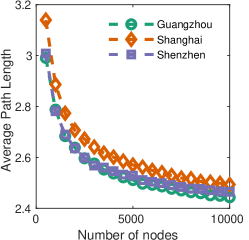
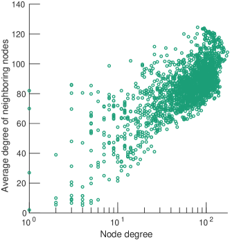
Despite the differences in scale and layout of the metro networks, we can immediately observe several structure properties that are universal across the MCNs. The MCNs of different cities and of various number of nodes all present high values of average clustering coefficient, short average path lengths and small network diameters. Moreover, these statistics are found to converge to fixed values with the number of nodes increases from 500 to 7,000 and then become invariant with further increases in the number of nodes in the network (see Fig. S2 for the convergence of average path length). These results suggest that the structural properties of the MCNs are primarily determined by the layout and scale of the metro network. And the minor differences in the values of these network metrics are also reflections of the differences in their metro systems. Since Shanghai has the largest metro network, we observe the average path length and the network diameter are in general higher than those of Guangzhou and Shenzhen, and the average clustering coefficient is comparatively lower than other cities due to more diverse destinations among travelers. Finally, the assortativity values of the three cities imply that MCNs are weakly assortative where nodes are likely to be connected to other nodes with similar degree and this can be verified from the visualization in Fig. S3. In general we observe a positive correlation between the node degree and the average degree of the neighboring nodes, but there is also huge discrepancy among the average degree of the neighboring nodes for the nodes of similar degree. This indicates certain level of randomness in the number of contacts in the MCN, which is likely to depend on the time of arrival and the specific pair of trip origin and destination.
S2.4 Network randomization
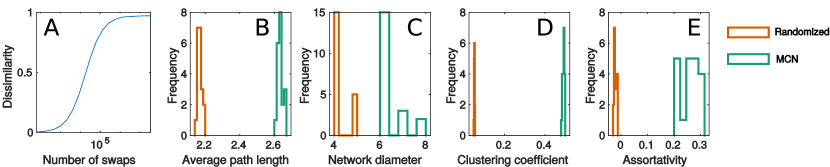
To verify the statistical significance of the network metrics for MCNs, we conduct the randomization of the simulated MCNs by selecting two random links in the MCN and swap their endpoints, which is also known as XSwap hanhijarvi2009randomization . XSwap produces the randomization of the MCN while preserving the same degree distribution. We compare the network metrics discussed above between 20 samples of MCN and the corresponding randomized networks, and the results are shown in Fig. S4. It is obvious that the differences in the distributions of network metrics between the two networks are statistically significant. This confirms the observed structural properties are distinct in MCNs. These results highlight that MCN is a special type of network that presents universal structural properties though being stemmed from metro systems of different scales and layouts.
S2.5 Degree distribution
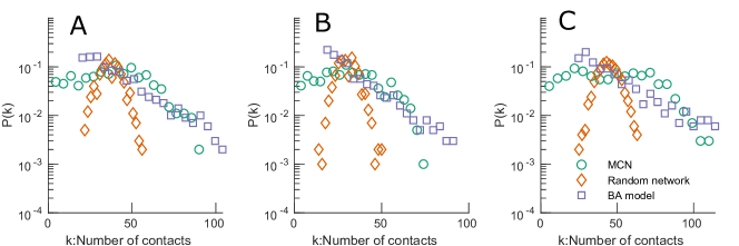
The universality of the MCN can also be observed from its unweighted and weighted degree distributions. We first observe that with the same number of nodes in MCNs, the average unweighted degree and weighted degree are different among the three cities. Shenzhen metro has the highest average unweighted and weighted node degree and also the largest variation of node degree, followed by Guangzhou and Shanghai respectively. This is likely because that Shenzhen has the smallest metro network among the three which results in higher chance of contact and hence higher clustering coefficient and average node degree. But the probability density function for the degree distributions of the three cities present striking similarities. As shown in Fig. S5, the unweighted degree distribution shows that there is large proportion of nodes of degree smaller or equal to around half of the maximum degree in MCN and it has a tail that decays almost exponentially fast. One may be tempted to fit a power-law distribution to explain the decay of the tail. Indeed, many real networks are observed to be well explained by power-law distribution and we observe alike decaying trend between MCN and the power-law counterpart. And the MCNs are shown to be significantly different from the random networks in terms of the overall shape and the tail behavior. But there are two subtle differences that prevents the use of power-law distribution for characterizing the degree distribution of MCNs. First, as seen in Fig. S5, the chance of having high-degree hubs in MCN is much lower as compared to the scale-free network of the same number of nodes and links. This indicates the decay of the tail is faster than that in the scale-free network. But more importantly is that MCNs are deemed to be scale-dependent and the degree distribution is closely associated with the number of nodes or equivalently the number of travelers in the metro system. This poses a fundamental contradiction to the philosophy behind the power-law distribution and its properties.
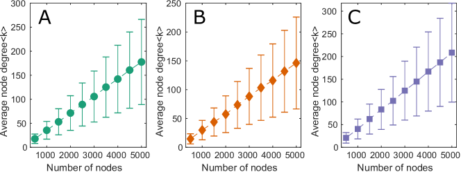
Nevertheless, the degree distribution of MCN presents several surprising properties that are usually seen in the scale-free network. The first is the possible divergence of and as shown in Fig. S6, where the standard deviation of the node degree increases with higher average node degree. Such phenomenon is one important reason that leads to the presence of scale-free property and this is observed in the MCNs for all three cities. In addition, despite seeing that the chance of large hubs is much lower in MCN than in the scale-free network, we empirically observe that the maximum degree of the MCN also increase linearly with increasing size of the network. This again is a unique property that is found in scale-free networks:
| (4) |
where is the exponent the power-law distribution.
In summary, by analyzing the simulated MCNs, we find that several structural properties of the MCNs are invariant to the size of the network and are primarily determined by the layout and scale of the metro systems. We show that these properties are rare in random networks and are likely to be distinct features of MCNs that are universal across different cities. But more importantly, while presenting fundamental differences when compared with scale-free networks, the MCNs also present universal structural properties that are usually found in scale-free networks. These findings define the MCN as a special class of networks that arises from the collective behavior of travelers and also the interplay between trip pattern and the metro system layout.
S3 Individual level disease transmission model
Based on the constructed MCNs, we next model the percolation of communicable diseases on the MCNs with the individual based model (IBM). The IBM is adapted from the non-linear dynamical system approach in chakrabarti2008epidemic . In the IBM, each traveler is a node in MCN and the transmission takes place between two travelers with positive . We consider the classical susceptible-infectious-susceptible (SIS) model as the disease dynamics, while a more refined model such as SIR and SEIR can also be embedded.
The IBM model takes the following items as model input:
-
1.
The unweighted adjacency matrix or weighted adjacency matrix of the MCN.
-
2.
Disease parameters: unit transmission rate and recovery rate , where represents the units number of time steps required for full recovery.
S3.1 Disease transmission rate
For communicable diseases that spread upon contact, it is well understood that the exposure duration and contact distance between two individuals are two contributing factors to a successful transmission. In our study, the strength of transmission between two individuals is denoted by equation 3. It measures the expected contact duration of two travelers based on their travel profile, and scales the probability of contact by considering the chance if two individuals are within effective transmission distance. As a consequence, we are able to measure the heterogeneous transmission rate between two travelers.
S3.2 The model
Denote as the probability that node is infected at time . When an individual travels, the probability that stays healthy at time can be written as:
| (5) |
where represents the probability that neighboring nodes of fail to transmit disease to node at time . The first term on right hand side of the equation implies the node was healthy at time and is not infected at time , and the second term suggests that the node was infected at time but recovered at time .
The probability that all neighbors of failed to transmit the disease can be written as:
| (6) |
with denotes the set of neighboring nodes of . The right hand side also also contains two parts: either a neighbor is not infectious at current time (), or if is infectious but fails to transmit the diseases.
By rearranging equation 5, we can express the probability that node is infected at time as
| (7) |
And the entire system dynamics over the MCN can be expressed in the matrix form as
| (8) |
So that the disease spreading on MCN is characterized as a non-linear dynamic system.
S3.3 Condition for disease free equilibrium
The disease dynamic system on MCN has two equilibrium states. One is the disease free equilibrium (DFE), where each individual is in S (healthy) state and the disease is completely eliminated. On the contrary is the endemic equilibrium, where there will always be a positive portion of nodes that are in I state. Formally, the DFE can be defined as
Definition 1 (Disease free equilibrium (DFE)).
The system reaches the disease free equilibrium if at time for all nodes.
The vulnerability of a metro system therefore corresponds to the stability condition for the IBM of the MCN to reach DFE. The stability of the system depends on how the system may return to equilibrium under small perturbation. If the perturbation diminishes and the system goes back to the equilibrium point, the DFE point is said to be asymptotically stable, otherwise the system will reach the endemic state. Before we establish the stability condition for DFE, we first introduce the Gershgorin Circle theorem golub2012matrix as follows
Theorem 1 (Gershgorin circle theorem).
Every eigenvalue of a complete matrix A lies within at least one of the Gershgorin discs :
| (9) |
where is the eigenvalue of .
Based on Gershgorin circle theorem, we develop the following condition for the stability of the DFE on MCN:
Proposition 1.
The DFE is asymptotically stable if .
Proof.
We proof the proposition by linearizing the non-linear dynamic system at the DFE and measuring the partial derivatives :
| (10) |
where we have
| (11) |
| (12) |
| (13) |
Therefore we have
| (14) |
For the DFE to be stable, it must be satisfied that the largest eigenvalue of is less than 1:
| (15) |
Define as an upper bound of the eigenvalue of . Since all diagonal entries of are identical, by applying Theorem 1, we have
| (16) |
To satisfy the condition in equation 15, we require the upper bound to satisfy:
| (17) |
This gives that and completes the proof. ∎
Proposition 1 has several important implications. The risk level of the MCN is shown to be dictated by the individual who has the highest risk exposure. As long as the exposure rate of this particular individual is smaller than the recovery speed, the system will reach DFE. Otherwise the system may be either DFE or endemic. However, in practice, if we would like to control the spread of communicable diseases, it is unlikely that we may identify who exactly this person is. Even if this person is spotted, vaccine/quarantine the individual does not necessarily reduce the risk level of the overall system, since the second riskiest person may have similar level of risk exposure. This implies that we would also need to examine the structure of the contact network to devise feasible control strategies. In addition, the model provides the solution to monitor the vulnerability of metro systems at very fine scale and identify the periods of time that are of particularly high risk level.
S4 OD-level model
One drawback of the IBM model, however, comes from its computational bottleneck. It will be very expensive to generate large-scale MCN with millions of passengers that copes with the passenger demand level in real-world scenarios. In this regard, we also develop a metapopulation model based on the flow of travelers between each pair of origin and destination (OD) pair. The OD level model can be used to monitor the risk level of metro systems, but it does not reveal any insights on the contact pattern among individual travelers. The OD-level model treats each pair of OD as the set of nodes and the contagion pattern between OD pairs as the set of links. It can be readily seen that the total number of OD pairs in a given metro network is the square of number of stations, which is much more scalable as compared to constructing contact networks for millions of travelers. Denote and as the susceptible population and infected population of OD pair , and let be the set of OD pairs in the network, we have the following equations
| (18) |
where represents the proportion of susceptible population of being infected by the infectious population of and is the expected contact duration between OD pairs and . The disease dynamics at the OD level can therefore be written as:
| (19) |
Moreover, since , where is the total number of travelers for OD pair , equation 19 can be further rewritten as:
| (20) |
And the matrix form is therefore
| (21) |
where is a square matrix with its entry: and . is a column vector with its entry being . Equation 21 gives the disease dynamics at the OD level.
We can see that one important difference between the OD-level model and the IBM is that the OD-level model use as the aggregate representation of the contact duration between all travelers of OD pair and travelers of OD pair , rather than the individual level contact duration between travelers and . As a result, it sacrifices the fidelity for modeling disease at the individual model, but can be used for understanding the system level dynamics more efficiently.
S5 Generation model
By observing that multiple metro networks in different cities share very similar degree distributions in their MCNs, we next establish the generation mechanism to model how the MCNs are shaped during travel. The goal is to build a single generation mechanism that is capable of restoring the MCNs of all cities to support the universality of MCNs.
Being different from many other networks, the MCNs are special in the way that the number of links each node being adjacent should be a function of the total number of nodes in the MCNs. This corresponds to the congestion effect in the metro system with more number of travelers. Consequently, the MCNs may not be generated in the way like preferential attachment newman2001clustering where new nodes and links are added sequentially. Instead, we follow a process where we first estimate the total number of links in the network and then assign the links among the nodes in a way similar to the configuration model.
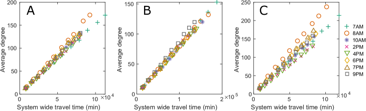
To cope with the congestion effect in MCNs, we consider the expected number of contacts each node may encounter as:
| (22) |
This states that the number of contacts is proportional to the rescaled travel time and the number of nodes . In particular, with , suggests more expected number of contacts with increasing travel time, and if we take the derivative of with respect to , we have
| (23) |
which implies that, in contrast to the rescale as , the number of contacts does not increase linearly with increasing . Instead, the increase rate will drop with the increase in travel time. Indeed, the number of contacts one may have with 40 minutes of travel should not be 10 times that of the number contacts as if one travels for 4 minutes. Regarding the value of , we define it as the similarity coefficient that measures the ’similarity’ of travels among all travelers. Higher value of indicates that, on average, a traveler will have higher contact chance with another traveler, e.g., two travelers are more likely to travel in the same direction to the same destination. On the other hand, the value of reflects the scale of the metro network, with the physical meaning being the contact rate per individual traveler per unit time of travel. As a result, is a system dependent value and varies across the cities.
With the above definition, we can approximate the total number of links (contacts) in the MCNs as:
| (24) |
And if we consider each link as two stubs (half links), denoting and , we then assign these stubs to each node based on their contribution , where the probability that a randomly chosen stub is adjacent to node with travel time as:
| (25) |
While each stub counts as one degree for each node, we can therefore write down the probability density function that a node of travel time is of degree follows the binomial distribution:
| (26) |
Then for a randomly selected node in the MCN, the probability density function for the number of contacts follows
| (27) |
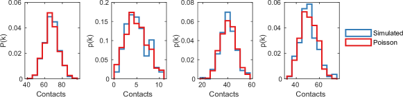
where is the probability density function for the human mobility within metro system and is observed to be well captured by the exponential distribution. With large , we can approximate the binomial distribution as the Poisson distribution and hence we have
| (28) |
and this gives the probability density function for the unweighted MCN.
Following equation 28, we can subsequently generate a MCN with stubs attached to each node. To produce the weighted MCN, we follow the process of the configuration model as:
-
1.
Randomly selected two stubs in the unweighted MCN, with the nodes adjacent to the stubs as and .
-
2.
Connect the selected stubs with an link, and assign the weight to the link: .
-
3.
Repeat the above two steps until all stubs are exhausted. Output the weighted MCN.
In summary, the above procedure describes the growth of MCN as a two-stage process where we first determine if two travelers will get into contact and then decide the duration of their contact which is assumed to be proportional to the shorter travel time of the two.
S5.1 Validation
The validation of the generation model involves the calibration of the model parameters and then verify if the calibrated generation model is representative of the simulated MCNs from the smart card data. To correctness of the generation model is validated using the two sample Kolmogorov–Smirnov (KS) test massey1951kolmogorov to compare the CDF of the degree distribution of the MCN from the generation model and the CDF of the degree distribution of the MCNs simulated from the smart card data. The null hypothesis of the KS test is that the two data samples for comparison are drawn from the same continuous distribution. Specifically, we binned the degree distribution of each MCN into 20 equal-length intervals, and conduct KS test on the probability distribution of the binned data.
The calibration of model parameters is to find the best and value that leads to the best goodness of fit between the generation model and the simulated MCNs. In particular, we have different for different time intervals while is held the same across all time intervals for a particular city. Since we do not have a closed form representation for the probability density function of the weighted MCNs, we conduct cross-validation to find the pair of parameters that minimizes the KS statistics. For each city, we consider being time invariant since it captures the impacts of metro network structure, and will change over time to reflect temporal variations of passenger trip patterns. We perform cross-validation to determine the optimal and for each city and for each time period, with the selection criteria being the parameter combination that gives the lowest sum of KS statistics for weighted degree distribution and unweighted degree distribution of the MCNs.
S5.2 Measure of similarity
To further validate the correctness of , we present the metric for measuring the trip similarity among all travelers and we compare the computed metrics to the fitted values. The similarity is measured by first constructing the correlation matrix of the trip pairs, where for each entry of :
| (29) |
where and represent the normalized trip flow traveling on OD pair and OD pair (number of nodes on OD pair divided by total number of nodes in MCN). refers to the standardized contact duration between the two OD pairs. In this regard, each entry of measures the pairwise contagion strength and row of therefore gives the level of correlation of OD pair with all other OD pairs. And the correlation depends on both the demand level as well as the contact duration.
Given the correlation matrix , we next extract the top eigenvalues of as , and we define similarity index as the standard deviation among the top eigenvalues:
| (30) |
where refers to the mean of the eigenvalues. With the normalization of trip flow and standardization of contact duration, we restrict to lie between 0 and 1.
The idea of similarity index is related to the principal component analysis of the correlation matrix, where the trace of the correlation matrix measures the total variance and the top principal components seek to maximize the variance. The standard deviation among the top eigenvalues therefore measures the differences in the total contribution to the total variance of each component, and hence reflects the trip differences among passengers. In particular, if those trips are totally uncorrelated and the trips, then the eigenvalues are all of the same value and the standard deviation among them is simply 0. An example in metro system is that the demand are evenly distributed among all OD pairs and these OD pairs have no overlapping segments to enable contacts. On the other hand, if some of the trip pairs are highly correlated, we should have few eigenvalues of value much higher than others, which gives rise to the large standard deviation. An extreme case in the metro system is that all travelers leave from the same origin to the same destination so that these trips are perfectly correlated and the standard deviation is therefore 1. The correlation matrix for metro systems is of size ( here is the number of stations) and we do not need to compute all eigenvalues. Instead, based on empirically observations, we find that eigenvalues drop quickly to nearly zero and we therefore set .
S6 First and second moment of node degree in MCN
Here we develop the first and second moment of the MCNs based on the generation model. We also derive an approximation of the largest node degree in a given MCN. These help to gain further insights on the degree distribution of the MCNs with increasing number of nodes.
S6.1 First moment
From the generation model for MCN we have:
| (31) |
And we can calculate the average degree of the MCN as:
| (32) |
When , the summation of discrete degree can be replaced with the integration:
| (33) |
where is the mean of the binomial distribution of trials and rate of success. And we therefore have:
| (34) |
Note that represents the probability density function for human mobility in metro network, which we find to be approximated by an exponentially decaying tail. We consider that
| (35) |
Then
| (36) |
Where the integration gives
| (37) |
where is the upper incomplete Gamma function with if , and . This suggests that
| (38) |
which suggests that the average degree of MCN is linearly proportional to the number of nodes in the network.
S6.2 Second moment
In addition, we can also calculate as
| (39) |
where represents the second moment of the binomial distribution. Following the same procedure for deriving , we arrive at the expression of as
| (40) |
This implies that the variance of MCN scales quadratically to the increase in number of nodes. These results explain the divergence of with .
S6.3 Max degree node
To estimate the maximum degree in MCN, let we consider the probability that
| (41) | ||||
where .
And for the maximum degree, we expect that
| (42) |
so that there is one node that is within the range . This condition suggests that
| (43) |
By taking the natural log on both sides, the equation simplifies to
| (44) | ||||
where for the last step we make use of the Taylor series expansion for log values
| (45) |
This result indicates that the maximum degree of the MCN is linearly proportional to the number of nodes in the network.
References
- [1] Gaode Map API. http://map.amap.com/subway/, 2018. Accessed: 2018-09-30.
- [2] Guangzhou metro timetable. http://cs.gzmtr.com/ckfw/fwsj/, 2018. Accessed: 2018-09-30.
- [3] Shanghai metro timetable. http://service.shmetro.com/en/hcskb/240.htm, 2018. Accessed: 2018-09-30.
- [4] Shenzhen metro timetable. http://www.szmc.net/page/eng/time_table.html, 2018. Accessed: 2018-09-30.
- [5] Jane D Siegel, Emily Rhinehart, Marguerite Jackson, and Linda Chiarello. 2007 guideline for isolation precautions preventing transmission of infectious agents in healthcare settings. 2007.
- [6] Duncan J Watts and Steven H Strogatz. Collective dynamics of ‘small-world’networks. nature, 393(6684):440, 1998.
- [7] Sami Hanhijärvi, Gemma C Garriga, and Kai Puolamäki. Randomization techniques for graphs. In Proceedings of the 2009 SIAM International Conference on Data Mining, pages 780–791. SIAM, 2009.
- [8] Deepayan Chakrabarti, Yang Wang, Chenxi Wang, Jurij Leskovec, and Christos Faloutsos. Epidemic thresholds in real networks. ACM Transactions on Information and System Security (TISSEC), 10(4):1, 2008.
- [9] Gene H Golub and Charles F Van Loan. Matrix computations, volume 3. JHU Press, 2012.
- [10] Mark EJ Newman. Clustering and preferential attachment in growing networks. Physical review E, 64(2):025102, 2001.
- [11] Frank J Massey Jr. The kolmogorov-smirnov test for goodness of fit. Journal of the American statistical Association, 46(253):68–78, 1951.