Multi-task Reinforcement Learning
with a Planning Quasi-Metric

Abstract

We introduce a new reinforcement learning approach combining a planning quasi-metric (PQM) that estimates the number of steps required to go from any state to another, with task-specific “aimers” that compute a target state to reach a given goal. This decomposition allows the sharing across tasks of a task-agnostic model of the quasi-metric that captures the environment’s dynamics and can be learned in a dense and unsupervised manner. We achieve multiple-fold training speed-up compared to recently published methods on the standard bit-flip problem and in the MuJoCo robotic arm simulator.

1 Introduction

We are interested in devising a new approach to reinforcement learning to solve multiple tasks in a single environment, and to learn separately the dynamic of the environment and the definitions of goals in it. A simple example would be a 2d maze, where there could be two different sets of tasks: reach horizontal coordinate $x$ or reach vertical coordinate $y$. Learning the spatial configuration of the maze would be useful for both sets of tasks.

Our approach relies on task-specific models which, given a starting state $s$, and a goal $g$ which is a set of states, compute a “target state” $s^{\prime}\in g$. We dubbed these models aimers (see § 2.2) and we stress that they are not designed to compute the series of actions to go from $s$ to $s^{\prime}$, but only $s^{\prime}$ itself. Given this target state, the planning per se is computed using a model of a quasi-metric between states (see § 2.1). This latter model is task agnostic and can be re-used from one to another. This decomposition allows to transfer the modeling of the world dynamic captured by the quasi metric, and to limit the task-specific learning to the aimers, which are lighter models trainable with very few observations as demonstrated in the experimental section (§ 3).

The idea of a quasi-metric between states is the natural extension of recent works, starting with the Universal Value Function Approximators (Schaul et al., 2015) which introduced the notion that learning the reward function can be done without a single privileged goal, and then extended with the Hindsight Experience Replay (Andrychowicz et al., 2017) that introduced the idea that goals do not have to be pre-defined but can be picked arbitrarily. Combined with a constant negative reward, this leads naturally to a metric where states and goal get a more symmetric role, which departs from the historical and classical idea of accumulated reward.

The long-term motivation of our approach is to segment the policy of an agent into a life-long learned quasi-metric, and a collection of task-specific easy-to-learn aimers. These aimers would be related to high-level imperatives for a biological system, triggered by low-level physiological necessities (“eat”, “get warmer”, “reproduce”, “sleep”), and high-level operations for a robot (“recharge battery”, “pick up boxes”, “patrol”, etc.). Additionally, the central role of a metric where the heavy lifting takes place provides a powerful framework to develop hierarchical planning, curiosity strategies, estimators of performance, etc.

Figure 1: Given a starting state $s$ and a goal $g\in{\cal G}$, the aimer $h^{{\cal G}}$ computes a target state $s^{\prime}$ which is the closest state in $g$, that is $s^{\prime}=h^{{\cal G}}(s,g)\in g$ that minimizes the length $\min_{a}f(s,s^{\prime}\!,a)$ of the dashed path to go from $s$ to $s^{\prime}$ under the environment dynamics.

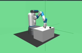
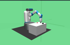
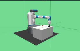
Figure 2: Trajectory of MuJoCo’s robotic arm when a new aimer is trained for the “push” task and the quasi-metric is kept from the “pick and place” task. The quasi-metric properly modeled how to move the arm at a desired location in contact with the black box, and needs minimal training to manipulate the box without gripper (see § 3.2.1).

2 Method

Let ${\cal S}$ be the state space and ${\cal A}$ the action space. We call goal a subset $g\subset{\cal S}$ of the state space, and a task a set of goals ${\cal G}\subset{\cal P}({\cal S})$. Many tasks can be defined in a given environment with the same state and action spaces. Note that in the environments we consider, the concrete definition of a task is a subset of the state vector coordinates, and a goal is defined by the target values for these coordinates.

Consider the robotic arm of the MuJoCo simulator (Todorov et al., 2012), that we use for experiments in § 3.2: The state space ${\cal S}$ concatenates, among others, the position and velocity of the arm and the location of the object to manipulate. Examples of tasks could be “reach a certain position”, in which case a goal is a set of states parameterized by a 3d position, where the position of the arm handle is fixed but all other degrees of freedom are let free, “reach a certain speed” where everything is let unconstrained but the handle’s speed, “put the object at the left side of the table”, where everything is free but one coordinate of the object location, and so on.

For what follows, we also let $(s_{t},a_{t},r_{t})\in{\cal S}\times{\cal A}\times\mathbb{R},\ t=1,\dots,T$ be a state / action / reward sequence.

2.1 Planning Quasi-Metric

Similarly to the distance between states proposed by Eysenbach et al. (2019), we explicitly introduce an action-parameterized quasi-metric

$$f:{\cal S}^{2}\times{\cal A}\rightarrow\mathbb{R}_{+}$$ (1)

such that $f(s,s^{\prime}\!,a)$ is “the minimum [expected] number of steps to go from $s$ to $s^{\prime}$ when starting with action $a$”.

We stress that it is a quasi-metric since it is not symmetric in most of the actual planning setups. Consider for instance one-way streets for an autonomous urban vehicle, irreversible physical transformations, or inertia for a robotic task, which may make going from $s_{1}=(x_{1},v_{1})$ to $s_{2}=(x_{2},v_{2})$ easy and the reciprocal transition difficult.

Given an arbitrary target state $s^{\prime}$, the update of $f$ should minimize

$$\left(f(s_{t},s_{t+1},a_{t})-1\right)^{2}+\left(f(s_{t},s^{\prime}\!,a_{t})-\left(1+\min_{\alpha}\tilde{f}(s_{t+1},s^{\prime}\!,\alpha)\right)\right)^{2}$$ (2)

where the first term makes the quasi-metric $1$ between successive states, and the second makes it globally consistent with the best policy, following Bellman’s equation. $\tilde{f}$ is a “target model”, usually updated less frequently or through a stabilizing moving average.

We implement the learning of the PQM with a standard actor/critic structure (Lillicrap et al., 2015). First the PQM itself that plays the role of the critic

$$f_{w_{f}}:{\cal S}^{2}\times{\cal A}\rightarrow\mathbb{R}_{+}$$ (3)

and an actor, which is either an explicit $\operatornamewithlimits{argmin}$ in the case of a finite set of actions, or a model

$$a_{w_{a}}:{\cal S}^{2}\rightarrow{\cal A}$$ (4)

to approximate $a_{w_{a}}(s,s^{\prime})\simeq\operatornamewithlimits{argmin}_{\alpha}f_{w_{f}}(s,s^{\prime},\alpha)$ when dealing with a continuous action space ${\cal A}.$

For training, given a tuple $(s_{t},s_{t+1},s^{\prime}\!,a_{t})$ we update $w_{f}$ to reduce

$$\mathcal{L}(w_{f};s_{t},s_{t+1},s^{\prime}\!,a_{t},\tilde{w}_{f})=\\ \left(f_{w_{f}}(s_{t},s_{t+1},a_{t})-1\right)^{2}+\left(f_{w_{f}}(s_{t},s^{\prime}\!,a_{t})\!-\!\left(1\!+\!f_{\tilde{w}_{f}}(s_{t+1},s^{\prime}\!,a_{\tilde{w}_{a}}(s_{t+1}s^{\prime}))\right)\right)^{2}\!\!\!$$ (5)

and we update $w_{a}$ to reduce

$$f_{w_{f}}(s_{t},s^{\prime}\!,a_{w_{a}}(s_{t},s^{\prime})),$$ (6)

so that $a_{w_{a}}$ gets closer to the choice of action at $s_{t}$ that minimizes the remaining distance to $s^{\prime}$.

2.2 Aimer

Note that while the quasi-metric allows to reach a certain state by choosing at any moment the action that decreases the distance to it the most, it does not allow to reach a more abstract “goal”, defined as a set of states. This objective is not trivial: the two objects are defined at completely different scales, the latter possibly ignoring virtually all the degrees of freedom of the former.

Hence, to use the PQM to actually reach goals, a key element is missing to pick the “ideal state” that (1) is in the goal but also (2) is the easiest to reach from the state currently occupied. For this purpose we introduce the idea of aimer (see figure 2) which, given a set of goals ${\cal G}\subset{\cal P}({\cal S})$, is of the form

$$h^{{\cal G}}:{\cal S}\times{\cal G}\rightarrow{\cal S}$$ (7)

and is such that $h^{{\cal G}}(s,g)$ is the “best” target state, that is the state in $g\in{\cal G}$ closest to $s$:

$$\forall s,g\in{\cal S}\times{\cal G},\ h^{{\cal G}}(s,g)=\operatornamewithlimits{argmin}_{s^{\prime}\in g}\min_{a}f(s,s^{\prime}\!,a).$$ (8)

The key notion in this formulation is that we can have multiple aimers dedicated to as many goal spaces, that utilize the same quasi-metric, which is in charge of the heavy lifting of “understanding” the underlying dynamics of the environment.

We follow the idea of the actor for the action choice, and do not implement the aimer by explicitly solving the system of equation 8 but introduce a parameterized model

$$h_{w_{h}}:{\cal S}\times{\cal G}\rightarrow{\cal S}.$$ (9)

For training, given a pair $(s,g)\in{\cal S}\times{\cal G}$ we update $w_{h}$ to reduce

$$f_{w_{f}}(s,h_{w_{h}}(s,g),a_{w_{a}}(s,h_{w_{h}}(s,g)))\\ +\lambda_{1}\,d(h_{w_{h}}(s,g),g)+\lambda_{2}\,v(h_{w_{h}}(s,g)).$$ (10)

The first term is an estimate of the objective of the problem (8), that is the distance between $s$ and $h_{w_{h}}(s,g)$, where the actor’s prediction plays the role of the $\min$ of the original problem.

The second term is a penalty replacing the hard constraints of (8) with a distance $d$ to a set. That latter distance is in practice a $L_{2}$ norm over a subset of the state’s coordinates. We come back to this with more details in § 3.

The third term $v$ is a penalty for imposing the validity of the state, for instance ensuring that speed or angles remain in valid ranges.

The resulting policy combines the actor $a$ and the aimer $h$. Given the current state $s$ and the goal $g$, the chosen action is $a(s,h(s,g))$.

3 Experiments

We have validated our approach experimentally in PyTorch (Paszke et al., 2019), on two standard environments: the bit-flipping problem (see § 3.1), known to be particularly challenging to traditional RL approaches relying on sparse rewards, and the MuJoCo simulator (see § 3.2), which exhibits some key difficulties of real robotic tasks. Our software to reproduce the experiments will be available under an open-source license at the time of publication.

To ensure that the benefits of PQM are complementary to state-of-the-art strategies making a smart re-use of episodes, we have compared our approach to the performance of DQN+HER from Andrychowicz et al. (2017) that we name here solely DQN for the bit-flipping problem and DDPG+HER from Plappert et al. (2018) that we name here solely DDPG for the Mujoco simulator. Hence all the algorithms we consider in the experimental part, both baselines and our PQM, are using HER.

The experimental results presented in this section were obtained with roughly 250 vCPU cores for one month, which is far less than the requirement for some state-of-the-art results. It forced us to only coarsely adapt configurations optimized in previous works for more classical and consequently quite different approaches.

3.1 Bit-flip

3.1.1 Environment and tasks

The state space for this first environment is a Boolean vector of $n$ bits, and there are $n$ actions, each switching one particular bit of the state. We fix $n=30$ and define two tasks, corresponding to reaching a target configuration respectively for the first $15$ bits and the last $15$ bits. A goal in these tasks is defined by the target configuration of $15$ bits.

The difficulty in this environment is the cardinality of the state space, the lack of geometrical structure, and the average time it takes to go from any state to any other state under a random policy.

To demonstrate the transferability of the quasi-metric, we also consider a task defined by the 15 first bits, with transfer from a task defined by the 15 last bits. After training an aimer and quasi-metric on one, we train a new aimer on the other but keep and fine-tune the parameters $w_{f}$ of the quasi-metric.

3.1.2 Network architectures and training

The critic is implemented as $f(s,s^{\prime},a)=\phi_{a}(s,s^{\prime})$, where $\phi$ is a ReLU MLP with $2n=60$ input units, one hidden layer with $256$ neurons, and $n=30$ outputs. As indicated in § 2.1, the actor for this environment is an explicit $\operatornamewithlimits{argmin}$ over the actions. The aimer $h$ is implemented also as a ReLU MLP with $n+n/2=45$ input units corresponding to the concatenation of a state and a goal definition, one hidden layer with $256$ neurons, and $n=30$ output neurons, with a final sigmoid non-linearity.

The length of an episode is equal to the number of bits in the goal, which is twice the median of the optimal number of actions. We kept the meta-parameters as selected by Plappert et al. (2018, appendix B), and chose $\lambda_{1}=100$. There is no term imposing the validity of the aimer output, hence no parameter $\lambda_{2}$.

Following algorithm S.1, we train for $500$ epochs, each consisting of running the policy for $16$ episodes and then performing $40$ optimization steps on minibatches of size $256$ sampled uniformly from a replay buffer consisting of $10^{6}$ transitions. We use the “future” strategy of HER for the selection of goals Andrychowicz et al. (2017). We update the target networks after every optimization step using the decay coefficient of $0.95$.

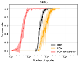
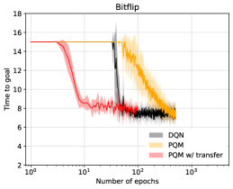
Figure 3: Empirical mean success rate (left) and median time to goal (right) with $\pm$ one standard deviation confidence interval on the bit-flip task (see § 3.1.1) of three different algorithms: a standard deep Q-learning (DQN), our approach that combines a planning quasi-metric with an aimer (PQM), and the same with training of an aimer from scratch and transfer of the quasi-metric trained on a task where the bits to match to reach the goals were different (PQM w/ transfer). That latter curve shows a boost in early training thanks to the pre-trained quasi-metric.

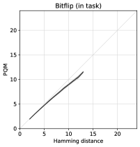
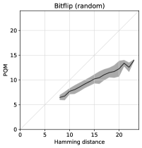
Figure 4: Accuracy of the quasi-metric estimate on the bit-flip task (see § 3.1.1). We plot here the empirical mean and $\pm$ one standard deviation confidence interval of the PQM estimate $\min_{a}f(s,s^{\prime},a)$ vs. the true distance, which here is the number of differing bits, hence the Hamming distance. The left figure is obtained when the starting state and the goal state differ only on the bits that are relevant to the task, hence are consistent with the aimer $h$, and the right figure when both are taken at random.

3.1.3 Results

The experiments in the bit-flip environment show the advantage of using a planning quasi-metric. As shown on figure 3, the training is successful and the combination of the quasi-metric and the aimer results in a policy similar to that of the standard DQN, both in terms of success rate and in terms of time to goal. It also appears that, while this model is slightly harder to train on a single task compared to DQN, it provides a great performance boost when transferring the PQM between tasks: since the quasi-metric is pre-trained, the training process only needs to train an aimer, which is a simple model, and fine-tune the quasi-metric.

It is noteworthy that due to limited computational means, we kept essentially the meta-parameters of the DQN setup of Andrychowicz et al. (2017), and as such the comparison is biased to DQN’s advantage.

Figure 4 gives a clearer view of the accuracy of the metric alone. We have computed after training the value of $\min_{a}f(s,s^{\prime},a)$ for pairs of starting states / target states taken at random, and compared it to the “true” distance, which happens to be in that environment the Hamming distance, that is the number of bits that differ between the two.

For the tasks in this environment, the aimer $h$ predicts a target state whose bits that matter for the task are the goal configuration, and the others are unchanged from the starting state, since this corresponds to the shortest path. Hence we considered two groups of state pairs: Either “in task”, which means that the two states are consistent with the aimer prediction in the task, and differ only on the bits that matter for the task, or “random” in which case they are arbitrary, and hence may be inconsistent with the biased statistic observed during training.

The results show that the estimate of the quasi-metric is very accurate on the first group, less so on the second, but still strongly monotonic. This is consistent with the transfer providing a substantial boost to the training on a new task.

3.2 MuJoCo

3.2.1 Environment and tasks

For our second set of experiments, we use the “Fetch” environments of OpenAI gym (Brockman et al., 2016) which use the MuJoCo physics engine (Todorov et al., 2012), pictured in figure 2, and are described in details by Plappert et al. (2018, section 1.1). If left unspecified the details of our experiments are the same as indicated by Plappert et al. (2018, section 1.4), and Andrychowicz et al. (2017, appendix A).

We consider two tasks: “push”, where a box is placed at random on the table and the robot’s objective is to move it to a desired location also on the table, without using the gripper, and “pick and place”, in which the robot can control its gripper, and the desired location for the box may be located above the table surface.

To demonstrate the transferability of the quasi-metric in this environment, we also consider the “push” task with transfer from “pick and place”: after training an aimer and the quasi-metric on the latter, we train a new aimer on the former, but keep the parameters $w_{f}$ and $w_{a}$ as starting point for the quasi-metric.

Note that our implementation of DDPG outperforms the results obtained by Plappert et al. (2018). This is due to the addition of an extra factor in the loss of the critic which sets the target Q value to 0 whenever the goal is reached. In our approach, the metric does not entail at all the notion of a goal, hence this factor was omitted.

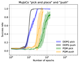
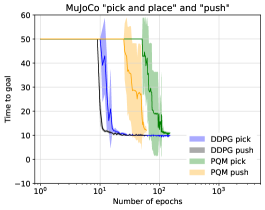
Figure 5: Empirical mean success rate (left) and median time to goal (right) with $\pm$ one standard deviation confidence interval on the MuJoCo “pick and place” and “push” tasks (see § 3.2.1). We compare the performance of the Deep Deterministic Policy Gradient (DDPG), with our approach that combines a planning quasi-metric with an aimer (PQM). These curves show that although the metric is harder to learn than the policy alone, the joint learning of the two models is successful.

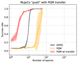
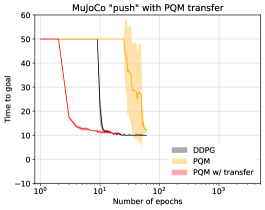
Figure 6: Empirical mean success rate (left) and median time to goal (right) with $\pm$ one standard deviation confidence interval on the MuJoCo “push” task (see § 3.2.1). We compare the performance of the Deep Deterministic Policy Gradient (DDPG), with our approach that combines a planning quasi-metric with a aimer (PQM), and the same with training of an aimer from scratch and transfer of the quasi-metric trained on the “pick and place” task (PQM w/ transfer). That latter curve shows a boost in early training thanks to the pre-trained quasi-metric.

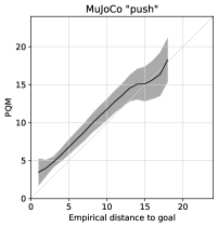
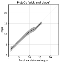
Figure 7: Accuracy of the quasi-metric on the MuJoCo “push” and “pick and place” tasks (see § 3.2.1). We plot here the empirical mean and $\pm$ one standard deviation confidence interval of the PQM estimate $f(s,s^{\prime},a(s,s^{\prime}))$ at the beginning of a successful episode, where $s^{\prime}$ is the target goal as estimated by the aimer vs. the actual number of steps it took to reach $s^{\prime}$.

3.2.2 Network architectures and training

In what follows let $d_{s}=25$ be the dimension of the state space ${\cal S}$, $d_{a}=4$ the dimension of the action space ${\cal A}$, $d_{g}=3$ the dimension of the goal parameter, which corresponds to the desired spatial location of the manipulated box.

The critic $f$ is implemented with a ReLU MLP, with $2d_{s}+d_{a}$ input units, corresponding to the concatenation of two states and an action, three hidden layers with $512$ units each, and a single output unit. The actor $a$ is a ReLU MLP with $2d_{s}$ input units, three hidden layers with $512$ units each, and $d_{a}$ output units with $\tanh$ non-linearity. As Plappert et al. (2018), we also add a penalty to the actor’s loss equal to the square of the output layer pre-activations. Finally the aimer $h$ is a ReLU MLP with $d_{s}+d_{g}$ input units, three hidden layers of $256$ units, and $d_{s}$ output units.

Following the algorithm S.1, for “pick and place” and “push with transfer”, we train for $150$ epochs. For “push”, we train for $60$ epochs. As in Plappert et al. (2018), each epoch consists of $50$ cycles, and each cycle consists of running the policy for $2$ episodes and then performing $40$ optimization steps on minibatches of size $256$ sampled uniformly from a replay buffer consisting of $10^{6}$ transitions. We use the “future” strategy of HER for the selection of goals (Andrychowicz et al., 2017), and update the target networks after every cycle using the decay coefficient of $0.95$.

We kept the meta-parameters as selected in Plappert et al. (2018, appendix B), with an additional grid search over the number of hidden neurons in the actor and critic models in $\{256,512\}$, $\lambda_{1}$ in $\{50,100,250,500,750,1000\}$, and $\lambda_{2}$ in $\{0,1,5,10,50,100,250,500,750,1000\}$.

For each combination, we trained a policy on the “push” task, and eventually selected the combination with the highest rolling median success rate over $10$ epochs, resulting in $512$ hidden neurons, $\lambda_{1}=500$, and $\lambda_{2}=50$. Note that additional trials tuning the learning rate of the models did not yield significant improvements.

All hyperparameters are described in greater detail by Andrychowicz et al. (2017).

3.2.3 Results

The results obtained in this environment confirm the observations from the bit-flip environment. Figure 5 shows that the joint training of the PQM and aimers works properly and results in a policy similar to that obtained with the DDPG approach. Once again, the PQM is slightly harder to train on a single task, in part due to the limited meta-optimization we could afford that favors the baseline, and in part due to the difficulty of learning the metric, which is a more complicated functional. However, our approach outperforms DDPG when the aimer alone has to be trained from scratch, and the PQM is transferred between tasks.

Figures 2 and 6 show the advantage of using the PQM to transfer knowledge from a task to another. Even though the two tasks are quite different, one using the gripper and moving the object in space while holding it, and the other moving only by contact in the plane, the quasi-metric provides an initial boost in the training by providing the ability to position the arm.

Finally, Figure 7 shows that the estimate of the quasi-metric accurately reflects the actual distance to the goal state.

4 Related works

The idea of a goal-conditioned policy combined with a constant negative reward, which results in an accumulated reward structure having the form of the [opposite of] the distance to the goal (Kaelbling, 1993) has seen a strong renewal of interest recently. Eysenbach et al. (2019) explicitly consider a distance between states, Hartikainen et al. (2019) utilize a learned distance function to efficiently optimize a goal-reaching policy and Dhiman et al. (2018) optimize a value function between states, which accounts for the distance function, based on the triangular inequality. As such, these works make use of a metric between states but do not use the notion of aimer in order to generate a state-goal to reach from the current state. While Nasiriany et al. (2019) and Florensa et al. (2019) use a similar concept to the aimer, it can in practice only generate nearby goals from the current state and there is no explicit transferability through a shared distance metric among different tasks.

The idea of transferring models has been applied to reinforcement learning Taylor and Stone (2009), with recent successes using a single model that mimics specialized expert actors on individual tasks Parisotto et al. (2016). The key issue of bringing several models to a common representation is tackled by normalizing contributions of the different tasks Hessel et al. (2018). This is in contrast with our proposal, which explicitly leverages being in a similar environment, and corresponds in our view to a more realistic robotic setup for which the embodiment is fixed.

More recently, Chen et al. (2019) address the transferability problem through the use of attention and planning modules. An embedding is learnt to go from a high dimensional continuous state space into a low dimensional discrete one in order to facilitate the planning process. Prior training of the policy and value function approximators is leveraged to reduce the number of required samples for solving new tasks. In a similar setting, Chiang et al. (2019) propose to learn a transferable obstacle avoiding state-to-state policy with evolutionary algorithms. From the rollouts generated, a time to reach estimator is learnt and used to grow a tree of nearby states to attain during the actual planning.

5 Conclusion

We have proposed to address the action selection problem by modeling separately the estimation of a target state given a goal and a quasi-metric between states. Experiments show that these two models can be trained jointly to get an efficient policy and that this approach supersedes robust baselines. As also illustrated in the experiments, the core advantage is that this decomposition moves the bulk of the modeling to the quasi-metric, which can be trained across tasks, with a dense feedback from the environment, while the aimer can be trained very quickly from a small number of episodes.

By disentangling two very different aspects of the planning, this decomposition is very promising for future extensions. The aimers are easier to learn and may be improved with a specific class of regressors taking advantage of a coarse-to-fine structure: your final destination can be initially coarsely defined and refined along your way. The quasi-metric handles the difficulty of learning a global structure known only through local interactions but is potentially amenable to the triangular inequality, clustering methods, and dimension reduction.

Broader Impact

For the past decade, Deep Reinforcement Learning has been paving the way towards Artificial General Intelligence. It is our belief that transfer learning and shared representations constitute a step in that direction.

Nonetheless, Deep Reinforcement Learning requires tremendous computational resources that only a few companies and institutions can afford. Our approach allows one to speedup the learning process thus lowering the entry barrier to practical applications and new research. Besides, power consumption has a direct environmental cost.

References

- Andrychowicz et al. (2017) M. Andrychowicz, F. Wolski, A. Ray, J. Schneider, R. Fong, P. Welinder, B. McGrew, J. Tobin, P. Abbeel, and W. Zaremba. Hindsight experience replay. CoRR, abs/1707.01495, 2017.
- Brockman et al. (2016) G. Brockman, V. Cheung, L. Pettersson, J. Schneider, J. Schulman, J. Tang, and W. Zaremba. Openai gym. CoRR, abs/1606.01540, 2016.
- Chen et al. (2019) B. Chen, B. Dai, and L. Song. Learning to plan via neural exploration-exploitation trees. CoRR, abs/1903.00070, 2019.
- Chiang et al. (2019) H. L. Chiang, J. Hsu, M. Fiser, L. Tapia, and A. Faust. Rl-rrt: Kinodynamic motion planning via learning reachability estimators from rl policies. IEEE Robotics and Automation Letters, 4(4):4298–4305, 2019.
- Dhiman et al. (2018) V. Dhiman, S. Banerjee, J. M. Siskind, and J. J. Corso. Floyd-warshall reinforcement learning learning from past experiences to reach new goals. CoRR, abs/1809.09318, 2018.
- Eysenbach et al. (2019) B. Eysenbach, R. Salakhutdinov, and S. Levine. Search on the replay buffer: Bridging planning and reinforcement learning. CoRR, abs/1906.05253, 2019.
- Florensa et al. (2019) C. Florensa, J. Degrave, N. Heess, J. T. Springenberg, and M. A. Riedmiller. Self-supervised learning of image embedding for continuous control. CoRR, abs/1901.00943, 2019.
- Hartikainen et al. (2019) K. Hartikainen, X. Geng, T. Haarnoja, and S. Levine. Dynamical distance learning for unsupervised and semi-supervised skill discovery. CoRR, abs/1907.08225, 2019.
- Hessel et al. (2018) M. Hessel, H. Soyer, L. Espeholt, W. Czarnecki, S. Schmitt, and H. van Hasselt. Multi-task deep reinforcement learning with popart. CoRR, abs/1809.04474, 2018.
- Kaelbling (1993) L. P. Kaelbling. Learning to achieve goals. In International Joint Conference on Artificial Intelligence, pages 1094–1098, 1993.
- Lillicrap et al. (2015) T. P. Lillicrap, J. J. Hunt, A. Pritzel, N. Heess, T. Erez, Y. Tassa, D. Silver, and D. Wierstra. Continuous control with deep reinforcement learning. arXiv preprint arXiv:1509.02971, 2015.
- Nasiriany et al. (2019) S. Nasiriany, V. H. Pong, S. Lin, and S. Levine. Planning with goal-conditioned policies, 2019.
- Parisotto et al. (2016) E. Parisotto, J. L. Ba, and R. Salakhutdinov. Actor-mimic: Deep multitask and transfer reinforcement learning. In International Conference on Learning Representations (ICLR), 2016.
- Paszke et al. (2019) A. Paszke, S. Gross, F. Massa, A. Lerer, J. Bradbury, G. Chanan, T. Killeen, Z. Lin, N. Gimelshein, L. Antiga, A. Desmaison, A. Kopf, E. Yang, Z. DeVito, M. Raison, A. Tejani, S. Chilamkurthy, B. Steiner, L. Fang, J. Bai, and S. Chintala. Pytorch: An imperative style, high-performance deep learning library. In Neural Information Processing Systems (NeurIPS), pages 8024–8035, 2019.
- Plappert et al. (2018) M. Plappert, M. Andrychowicz, A. Ray, B. McGrew, B. Baker, G. Powell, J. Schneider, J. Tobin, M. Chociej, P. Welinder, V. Kumar, and W. Zaremba. Multi-goal reinforcement learning: Challenging robotics environments and request for research. CoRR, abs/1802.09464, 2018.
- Schaul et al. (2015) T. Schaul, D. Horgan, K. Gregor, and D. Silver. Universal value function approximators. In International Conference on Machine Learning (ICML), volume 37, pages 1312–1320, 2015.
- Taylor and Stone (2009) M. E. Taylor and P. Stone. Transfer learning for reinforcement learning domains: A survey. Journal of Machine Learning Research (JMLR), 10:1633–1685, 2009.
- Todorov et al. (2012) E. Todorov, T. Erez, and Y. Tassa. Mujoco: A physics engine for model-based control. In International Conference on Intelligent Robots and Systems, pages 5026–5033, 2012.