Inference for Batched Bandits

Abstract

As bandit algorithms are increasingly utilized in scientific studies and industrial applications, there is an associated increasing need for reliable inference methods based on the resulting adaptively-collected data. In this work, we develop methods for inference on data collected in batches using a bandit algorithm. We first prove that the ordinary least squares estimator (OLS), which is asymptotically normal on independently sampled data, is not asymptotically normal on data collected using standard bandit algorithms when there is no unique optimal arm. This asymptotic non-normality result implies that the naive assumption that the OLS estimator is approximately normal can lead to Type-1 error inflation and confidence intervals with below-nominal coverage probabilities. Second, we introduce the Batched OLS estimator (BOLS) that we prove is (1) asymptotically normal on data collected from both multi-arm and contextual bandits and (2) robust to non-stationarity in the baseline reward.

1 Introduction

Due to their regret minimizing guarantees bandit algorithms have been increasingly used in in real-world sequential decision-making problems, like online advertising [28], mobile health [44], and online education [36]. However, for many real-world problems it is not enough to just minimize regret on a particular problem instance. For example, suppose we have run an online education experiment using a bandit algorithm where we test different types of teaching strategies. When designing a new online course, ideally we could use the data from the previous experiment to inform the design, e.g., under-performing arms could be eliminated or modified. Moreover, to help others designing online courses we would like to be able to publish our findings about how different teaching strategies compare in their performance. This example demonstrates the need for statistical inference methods on bandit data, which allow practitioners to draw generalizable knowledge from the data they have collected (e.g., how much better one teaching strategy is compared to another) for the sake of scientific discovery and informed decision making.

In this work we will focus on methods to construct confidence intervals for the margin—the difference in expected rewards of two bandit arms—from batched bandit data. Rather than constructing high probability confidence intervals, we are interested in constructing confidence intervals by using the asymptotic distribution of estimators to approximate their finite sample distribution. Asymptotic approximation methods for statistical inference has a long history of being successful in science and leads to much narrower confidence intervals than those constructed using high probability bounds. Most statistical inference methods based on asymptotic approximation assume that treatments are assigned independently [15]. However, bandit data violates this independence assumption because it is collected adaptively, meaning previous actions and rewards inform future action selections. The non-independence makes statistical inference more challenging, e.g., estimators like the sample mean are often biased on bandit data [34, 39].

Throughout, we focus on the batched bandit setting, in which arms of the bandit are pulled in batches. For our asymptotic analysis we fix the total number of batches, $T$, and allow the arm pulls in each batch, $n$, to go to infinity. Note that we do not need or expect $n$ to go to infinity for real-world experiments; we use the asymptotic distribution of estimators to approximate their finite-sample distribution when constructing confidence intervals. We focus on the batched setting because it closely reflects many of the problem settings where bandit algorithms are applied. For example, in many mobile health [44, 24, 29] and online education problems [22, 36] multiple users use apps / take courses simultaneously, so a batch corresponds to the number of unique users the bandit algorithm acts on at once. The batched setting is even common in online recommendations and advertising because it is impractical to update the bandit after every action if many users visit the site simultaneously [40, 38, 12, 27]. In many such experimental settings the length of the study, $T$, cannot be arbitrarily adjusted, e.g., in online education, courses generally cannot be made arbitrarily long, and clinical trials often run for a standard amount of time that depends on the domain science (e.g. the length of mobile health studies is a function of the scientific community’s belief in how long it should take for users to form a habit). On the other hand, the number of users, $n$, can in principle grow as large as funding allows.

Additionally, in our batched setting, we assume that the means of the arms can change over time, i.e., from batch to batch, which reflects the temporal non-stationarity that is prevalent in many real world bandit application problems. For example, in online recommendation systems, the click through rate of a given recommendation typically varies over time, e.g., breaking news articles become less popular over time [40, 27]. Online education and mobile health are also highly non-stationary problems because users tend to disengage over time, so the same notification may be much less effective if sent near the end of an experiment than sent near the beginning [9, 21, 7]. Our statistical inference method does not need to assume that the number of stationary time periods in the experiment is large and is robust to temporal non-stationarity from batch to batch.

The first contribution of this work is proving that on bandit data, rather surprisingly, whether standard estimators are asymptotically normal can depend on whether the margin is zero. We prove that for common bandit algorithms, the arm selection probabilities only concentrate if there is a unique optimal arm. Thus, for two-arm bandits, the arm selection probabilities do not concentrate when the margin—the difference in the expected rewards between the arms—is zero. We show that this leads the ordinary least squares (OLS) estimator to be asymptotically normal when the margin is non-zero, and asymptotically not normal when the margin is zero. Since the OLS estimator does not converge uniformly (over values of the margin), standard inference methods (normal approximations, bootstrap) can lead to inflated Type-1 error and unreliable confidence intervals on bandit data.

The second contribution of this work is introducing the Batched OLS (BOLS) estimator, which can be used for reliable inference—even in non-stationary settings—on data collected with batched bandits. We prove that, regardless of whether the margin is zero or not, the BOLS estimator for the margin for both multi-arm and contextual bandits is asymptotically normal and thus can be used for both hypothesis testing and obtaining confidence intervals. Moreover, BOLS is also automatically robust to non-stationarity in the rewards and can be used for constructing valid confidence intervals even if there is non-stationarity in the baseline reward, i.e., if the rewards of the arms change from batch to batch, but the margin remains constant. If the margin itself is also non-stationary, BOLS can also be used for constructing simultaneous confidence intervals for the margins for each batch.

2 Related Work

Batched Bandits   Much work on batched bandits focuses on minimizing regret [35, 10] or identifying the best arm with high probability [2, 18]. The best arm identification literature utilizes high probability confidence bounds to construct confidence intervals for bandit parameters; we will discuss this method in the next section. Note that in contrast to other batched bandit literature that allow batch sizes to be adjusted adaptively [35], here we do not have adaptive control over the batch sizes.

Batched bandits are closely related to multistage adaptive clinical trials, in which between each batch (or stage of the trial) the data collection procedure can be adjusted depending on the outcome of the previous batches. Our Batched OLS estimator is most closely related to “stage-wise" p-values for group sequential trials that are computed on each stage separately [42]. p-value combination tests are commonly used to combine stage-wise p-values, when the sequence of p-values are shown to be independent or p-clud, meaning that under the null each p-value has a Uniform(0,1) distribution conditional on past p-values [42]. [31] formally establish the independence of stage-wise p-values for two-stage trials in which there are a countable number of adaptive rules; note that this rules out bandit algorithms with real-valued arm selection probabilities, like Thompson Sampling. [4] establishes the p-clud property for two-stage adaptive clinical trials under the assumption that the distribution of the second stage data is known conditioned on the decision rule and first stage data under the null hypothesis. Neither of these methods are sufficient for obtaining independent p-values for adaptive trials (1) with an arbitrary number of stages, (2) where exact distribution of rewards is unknown, and (3) where the action selection probabilities can be real numbers, like for Thompson Sampling.

High Probability Confidence Intervals   High probability confidence intervals provide stronger guarantees than those constructed using asymptotic approximations. In particular, these bounds are guaranteed to hold for finite number of observations and often even hold uniformly over all $n$ and $T$. These types of bounds are used throughout the bandit and reinforcement learning literature to construct confidence intervals for bandit parameters [14, 20], prove regret bounds [1, 26], and provide guarantees regarding best arm identification [16, 17]. The primary drawback of high probability confidence intervals is that they are much more conservative than those constructed using asymptotic approximations. This means that many more observations will be needed to get a confidence interval of the same width or for a statistical test to have the same power when using high probability confidence intervals compared to those constructed using asymptotic approximation. Since the cost of increasing the the number of users in a study can be large, being able to construct narrow—yet reliable—confidence intervals is crucial to many applications.

In our simulations we compare our method to high probability confidence bounds constructed using the self-normalized martingale bound of [1]. This bound is guaranteed to hold on adaptively collected data and is commonly used in the proof of regret bounds for bandit algorithms. We find that all the approaches based on asymptotic approximations (which we discuss next), significantly outperform the statistical test constructed using a self-normalized martingale bound in terms of power. Moreover, despite the weaker guarantees of statistical inference based on asymptotic approximations, they are generally able to provide reliable coverage of confidence intervals and type-1 error control.

Adaptive Inference based on Asymptotic Approximations   A common approach in the literature for performing inference on bandit data is to use adaptive weights, which are weights that are a function of the history. An early example of using adaptive weights is that of [33] and [32], who use adaptive weights in estimating the expected reward under the optimal policy when one has access to i.i.d. observational data. They use an Augmented-Inverse-Probability-Weighted estimator with adaptive weights that are a function of the estimated standard deviation of the reward. [32] conjecture that their approach can be adapted to the adaptive sampling case. Subsequently [11] developed the adaptively weighted method for inference on bandit data to produce the Adaptively-Weighted Augmented-Inverse-Probability-Weighted Estimator (AW-AIPW) for data collected via multi-arm bandits. They prove a central limit theorem (CLT) for AW-AIPW when the adaptive weights satisfy certain conditions. Note, however, the AW-AIPW estimator does not have guarantees in non-stationary settings.

Adaptive weights are also used by [6] to form the W-decorrelated estimator, a debiased version of OLS, that is asymptotically normal. In the multi-arm bandit setting, the adaptive weights are a function of the number of times an arm was chosen previously. We found that in the two-arm setting, the W-decorrelated estimator down-weights rewards from later in the study (Appendix F). [5] introduce the Online Debiased Estimator that also has bias guarantees on adaptive data, but in the more challenging high-dimensional linear regression setting. They prove the asymptotic normality of their estimator in the Gaussian autoregressive time series and the two-batch settings. Note that none of these estimation methods have guarantees in non-stationary bandit settings.

[25] provide conditions under which the OLS estimator is asymptotically normal on adaptively collected data. However, as noted in [41, 6, 11], classical inference techniques developed for i.i.d. data often empirically have inflated Type-1 error on bandit data. In Section 4.1, we discuss the restrictive nature of [25]’s CLT conditions.

3 Problem Formulation

Setup and Notation

Though our results generalize to $K$-arm, contextual bandits (see Section 5.2), we first focus on the two-arm bandit for expositional simplicity. Suppose there are $T$ timesteps or batches in a study. In each batch $t\in[1\colon T]$, we select $n$ binary actions $\{A_{t,i}\}_{i=1}^{n}\in\{0,1\}^{n}$. We then observe independent rewards $\{R_{t,i}\}_{i=1}^{n}$, one for each action selected. Note that the distribution of these random variables changes with the batch size, $n$. For example, the distribution of the actions one chooses for the $2^{\textnormal{nd}}$ batch, $\{A_{2,i}\}_{i=1}^{n}$, may change if one has observed $n=10$ vs. $n=100$ samples $\{A_{1,i},R_{1,i}\}_{i=1}^{n}$ in the first batch. For readability, we omit indexing random variables by $n$, except for the variables $H_{t-1}^{(n)}$ and $\pi_{t}^{(n)}$, and filtrations like $\mathcal{G}_{t-1}^{(n)}$ to be introduced next.

For each $t\in[1\colon T]$, the bandit selects actions $\{A_{t,i}\}_{i=1}^{n}\overset{i.i.d.}{\sim}\textnormal{Bernoulli}(\pi_{t}^{(n)})$ conditional on $H_{t-1}^{(n)}:=\{A_{t^{\prime},i},R_{t^{\prime},i}\}_{i=1,t^{\prime}=1}^{i=n,t^{\prime}=t-1}$, the history prior to batch $t$. Note, the action selection probability $\pi_{t}^{(n)}:=\mathbb{P}(A_{t,i}=1|H_{t-1}^{(n)})$ depends on the history $H_{t-1}^{(n)}$. We assume the following conditional mean for rewards:

$$\mathbb{E}\big{[}R_{t,i}\big{|}H_{t-1}^{(n)},A_{t,i}\big{]}=(1-A_{t,i})\beta_{t,0}+A_{t,i}\beta_{t,1}.$$ (1)

Note in equation (1) we condition on $H_{t-1}^{(n)}$ because the conditional mean of the reward does not depend on prior rewards or actions. Let $\textbf{X}_{t,i}:=[1-A_{t,i},A_{t,i}]^{\top}\in^{2}$; note $\textbf{X}_{t,i}$ is higher dimensional when we add more arms and/or context variables. We define the errors as $\epsilon_{t,i}:=R_{t,i}-(\textbf{X}_{t,i})^{\top}\boldsymbol{\beta}_{t}$. Equation (1) implies that $\{\epsilon_{t,i}:i\in[1\colon n],t\in[1\colon T]\}$ are a martingale difference array with respect to the filtration $\{\mathcal{G}_{t}^{(n)}\}_{t=1}^{T}$, where $\mathcal{G}_{t}^{(n)}:=\sigma\big{(}H_{t-1}^{(n)}\cup\{A_{t,i}\}_{i=1}^{n}\big{)}$; thus, $\mathbb{E}[\epsilon_{t,i}|\mathcal{G}_{t-1}^{(n)}]=0,\forall t,i,n$. The parameters $\boldsymbol{\beta}_{t}=(\beta_{t,0},\beta_{t,1})$ can change across batches $t\in[1\colon T]$, which allows for non-stationarity between batches. Assuming that $\boldsymbol{\beta}_{t}=\boldsymbol{\beta}_{t^{\prime}}$ for all $t,t^{\prime}\in[1\colon T]$ simplifies to the stationary mean case.

Action Selection Probability Constraint (Clipping)

In order to perform inference on bandit data it is necessary to guarantee that the bandit algorithm explores sufficiently. For example, the CLTs for both the W-decorrelated [6] and the AW-AIPW [11] estimators have conditions that implicitly require that the bandit algorithms cannot sample any given action with probability that goes to zero or one arbitrarily fast. Greater exploration also increases the power of statistical tests regarding the margin [43]. Moreover, if there is non-stationarity in the margin between batches, it is desirable for the bandit algorithm to continue exploring. We explicitly guarantee exploration by constraining the probability that any given action can be sampled (see Definition 1). We allow the action selection probabilities $\pi_{t}^{(n)}$ to converge to $0$ and/or $1$ at some rate.

Definition 1.

A clipping constraint with rate $f(n)$ means that $\pi_{t}^{(n)}$ satisfies the following:

$$\lim_{n\to\infty}\mathbb{P}\big{(}\pi_{t}^{(n)}\in[f(n),1-f(n)]\big{)}=1$$ (2)

4 Asymptotic Distribution of the Ordinary Least Squares Estimator

Suppose we are in the stationary case, and we would like to estimate $\boldsymbol{\beta}$. Consider the OLS estimator: $\boldsymbol{\hat{\beta}}^{\textnormal{OLS}}=(\underline{\textbf{X}}^{\top}\underline{\textbf{X}})^{-1}\underline{\textbf{X}}^{\top}\textbf{R}$, where $\underline{\textbf{X}}:=[\textbf{X}_{1,1},..,\textbf{X}_{1,n},..,\textbf{X}_{T,1},..,\textbf{X}_{T,n}]^{\top}\in^{nT\times 2}$ and $\textbf{R}:=[R_{1,1},..,R_{1,n},..,R_{T,1},..,R_{T,n}]^{\top}\in^{nT}$. Note that $\underline{\textbf{X}}^{\top}\underline{\textbf{X}}=\sum_{t=1}^{T}\sum_{i=1}^{n}\textbf{X}_{t,i}\textbf{X}_{t,i}^{\top}$.

4.1 Conditions for Asymptotically Normality of the OLS estimator

If $(\textbf{X}_{t,i},\epsilon_{t,i})$ are i.i.d., $\mathbb{E}[\epsilon_{t,i}]=0$, $\mathbb{E}[\epsilon_{t,i}^{2}]=\sigma^{2}$, and the first two moments of $\textbf{X}_{t,i}$ exist, a classical result from statistics [3] is that the OLS estimator is asymptotically normal, i.e., as $n\to\infty$,

$$(\underline{\textbf{X}}^{\top}\underline{\textbf{X}})^{1/2}(\boldsymbol{\hat{\beta}}^{\textnormal{OLS}}-\boldsymbol{\beta})\overset{D}{\to}\mathcal{N}(\boldsymbol{0},\sigma^{2}\underline{\boldsymbol{I}}_{p}).$$

[25] generalize this result by proving that the OLS estimator is still asymptotically normal in the adaptive sampling case when $\underline{\textbf{X}}^{\top}\underline{\textbf{X}}$ satisfies a certain stability condition. To show that a similar result holds for the batched setting, we generalize the CLT of [25] to triangular arrays (required since the distribution of our random variables vary as the batch size, $n$, changes), as stated in Theorem 5.

Condition 1 (Moments).

For all $t,n,i$, $\mathbb{E}[\epsilon_{t,i}^{2}\big{|}\mathcal{G}_{t-1}^{(n)}]=\sigma^{2}$ and $\mathbb{E}\big{[}\epsilon_{t,i}^{4}\big{|}\mathcal{G}_{t-1}^{(n)}\big{]}<M<\infty$.

Condition 2 (Stability).

For some non-random sequence of scalars $\{a_{i}\}_{i=1}^{\infty}$, as $n\to\infty$,

$a_{n}\cdot\frac{1}{nT}\sum_{t=1}^{T}\sum_{i=1}^{n}A_{t,i}\overset{P}{\to}1$

Theorem 1 (Triangular array version [25], Theorem 3).

Assuming Conditions 1 and 2, as $n\to\infty$,

$\big{(}\underline{\textbf{X}}^{\top}\underline{\textbf{X}}\big{)}^{1/2}(\boldsymbol{\hat{\beta}}^{\textnormal{OLS}}-\boldsymbol{\beta})\overset{D}{\to}\mathcal{N}(0,\sigma^{2}\underline{\textbf{I}}_{p})$.

Note that in the bandit setting, Condition 2 means that prior to running the experiment, the asymptotic rate at which arms will be selected is predictable. We will show that Condition 2 is in a sense necessary for the asymptotic normality of OLS. In Corollary 1 below we state that Conditions 1 and 3, and a non-zero margin are sufficient for stability Condition 2. Later, we will show that when the margin is zero, Condition 2 does not hold for many common bandit algorithms and prove that this leads the OLS estimator to be asymptotically non-normal.

Condition 3 (Conditionally i.i.d. actions).

For each $t\in[1\colon T]$, $\{A_{t,i}\}_{i=1}^{n}\overset{i.i.d.}{\sim}\textnormal{Bernoulli}(\pi_{t}^{(n)})$ i.i.d. over $i\in[1\colon n]$ conditional on $H_{t-1}^{(n)}$.

Corollary 1 (Sufficient conditions for Theorem 5).

If Conditions 1 and 3 hold, and the margin is non-zero, data collected in batches using $\epsilon$-greedy, Thompson Sampling, or UCB with clipping constraint with $f(n)=c~{}$ for some $0<c\leq\frac{1}{2}$ (see Definition 1) satisfy Theorem 5 conditions.

Figure 1: Empirical distribution of the Z-statistic ($\sigma^{2}$ is known) of the OLS estimator for the margin. All simulations are with no margin ($\beta_{1}=\beta_{0}=0$); $\mathcal{N}(0,1)$ rewards; $T=25$; and $n=100$. For $\epsilon$-greedy, $\epsilon=0.1$.

4.2 Asymptotic Non-Normality under No Margin

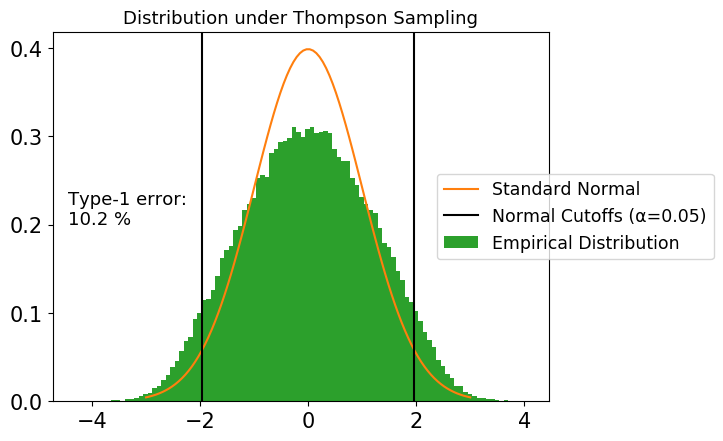
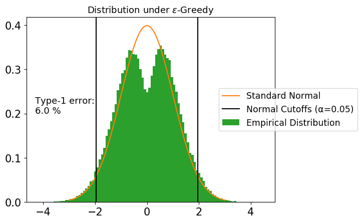
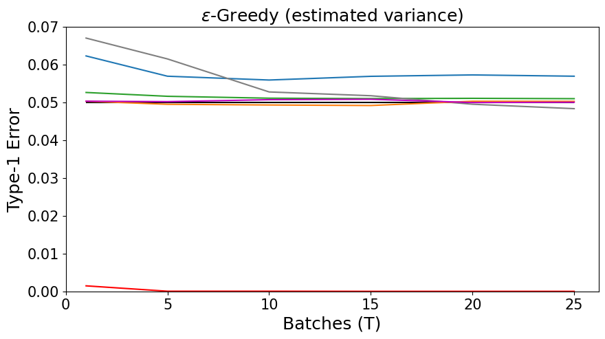
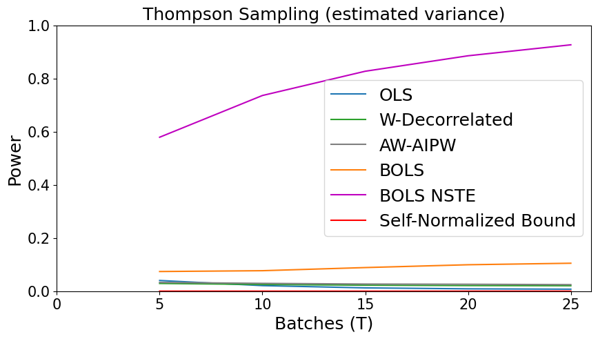
We prove the conjecture of [6] that when the margin is zero, the OLS estimator is asymptotically non-normal under common bandit algorithms, including Thompson Sampling, $\epsilon$-greedy, and UCB. Thus as seen in Figure 1, assuming the OLS estimator is approximately Normal on bandit data can lead to inflated Type-1 error, even asymptotically. The asymptotic non-normality of OLS occurs when the margin is zero because when there is no unique optimal arm, $\pi_{t}^{(n)}$ does not concentrate as $n\to\infty$ (Appendix C).

We state the asymptotic non-normality result for Thompson Sampling in Theorem 2; see Appendix C for the proof and similar results for $\epsilon$-greedy and UCB. It is sufficient to prove asymptotic non-normality for $T=2$. Note, $\hat{\Delta}^{\textnormal{OLS}}$ is the difference in the sample means for each arm, so $\hat{\Delta}^{\textnormal{OLS}}=\hat{\beta}_{1}^{\textnormal{OLS}}-\hat{\beta}_{0}^{\textnormal{OLS}}$. The Z-statistic of $\hat{\Delta}^{\textnormal{OLS}}$, which is asymptotically normal under i.i.d. sampling, is as follows:

$$\sqrt{\frac{\sum_{t=1}^{2}\sum_{i=1}^{n}A_{t,i})(\sum_{t=1}^{2}\sum_{i=1}^{n}1-A_{t,i})}{2\sigma^{2}n}}\big{(}\hat{\Delta}^{\textnormal{OLS}}-\Delta\big{)}.$$ (3)

Theorem 2 (Asymptotic non-normality of OLS estimator under zero margin for Thompson Sampling).

Let $T=2$ and $\pi_{1}^{(n)}=\frac{1}{2}$. If $\epsilon_{t,i}\overset{i.i.d.}{\sim}\mathcal{N}(0,1)$, we have independent normal priors on arm means $\tilde{\beta}_{0},\tilde{\beta}_{1}\overset{i.i.d.}{\sim}\mathcal{N}(0,1)$, and $\pi_{2}^{(n)}=\pi_{\min}\vee[(1-\pi_{\max})\wedge\mathbb{P}(\tilde{\beta}_{1}>\tilde{\beta}_{0}\big{|}H_{1}^{(n)})]$ for constants $\pi_{\min},\pi_{\max}$ with $0<\pi_{\min}\leq\pi_{\max}<1$, then (3) is asymptotically not normal when the margin is zero.

Figure 2: Empirical undercoverage probabilities (coverage probability below $95\%$) of confidence intervals using on a normal approximation for the OLS estimator. We use Thompson Sampling with $\mathcal{N}(0,1)$ priors, a clipping constraint of $0.05\leq\pi_{t}^{(n)}\leq 0.95$, $\mathcal{N}(0,1)$ rewards, $T=25$, and known $\sigma^{2}$. Standard errors are $<0.001$.

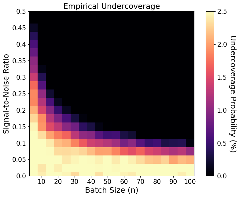
Since the OLS estimator is asymptotically normal when $\Delta\neq 0$ (Corollary 1) and asymptotically not Normal when $\Delta=0$, the OLS estimator does not converge uniformly on data collected under standard bandit algorithms. The non-uniform convergence of the OLS estimator precludes us from using a normal approximation to perform hypothesis testing and construct confidence intervals (see [19]). In real-world applications, there is rarely exactly zero margin. However, the non-uniform convergence of the OLS estimator at zero margin is still practically important because the asymptotic distribution of the OLS estimator when the margin is zero is indicative of the finite-sample distribution when the margin is statistically difficult to differentiate from zero, i.e., when the signal-to-noise ratio, $\frac{|\Delta|}{\sigma}$, is low. Figure 2 shows that even when the margin is non-zero, when the signal-to-noise ratio is low, confidence intervals constructed using a normal approximation have coverage probabilities below the nominal level. Moreover, for any batch size $n$ and noise variance $\sigma^{2}$, there exists a non-zero margin size with a finite-sample distribution that is poorly approximated by a normal distribution.

5 Batched OLS Estimator

5.1 Batched OLS Estimator for Multi-Arm Bandits

We now introduce the Batched OLS (BOLS) estimator that is asymptotically normal under a large class of bandit algorithms, even when the margin is zero. Instead of computing the OLS estimator on all the data, we compute the OLS estimator for each batch and normalize it by the variance estimated from that batch. For each $t\in[1\colon T]$, the BOLS estimator of the margin $\Delta_{t}:=\beta_{t,1}-\beta_{t,0}$ is:

$$\hat{\Delta}_{t}^{\textnormal{BOLS}}=\frac{\sum_{i=1}^{n}(1-A_{t,i})R_{t,i}}{\sum_{i=1}^{n}1-A_{t,i}}-\frac{\sum_{i=1}^{n}A_{t,i}R_{t,i}}{\sum_{i=1}^{n}A_{t,i}}.$$

Theorem 3 (Asymptotic Normality of Batched OLS estimator for multi-arm bandits).

Assuming Conditions 1 (moments) and 3 (conditionally i.i.d. actions), and a clipping rate $f(n)=\frac{1}{n^{\alpha}}$  for some $0\leq\alpha<1$ (see Definition 1),

$$\begin{bmatrix}\sqrt{\frac{(\sum_{i=1}^{n}1-A_{1,i})(\sum_{i=1}^{n}A_{1,i})}{n}}(\hat{\Delta}_{1}^{\textnormal{BOLS}}-\Delta_{1})\\ \sqrt{\frac{(\sum_{i=1}^{n}1-A_{2,i})(\sum_{i=1}^{n}A_{2,i})}{n}}(\hat{\Delta}_{2}^{\textnormal{BOLS}}-\Delta_{2})\\ \vdots\\ \sqrt{\frac{(\sum_{i=1}^{n}1-A_{T,i})(\sum_{i=1}^{n}A_{T,i})}{n}}(\hat{\Delta}_{T}^{\textnormal{BOLS}}-\Delta_{T})\\ \end{bmatrix}\overset{D}{\to}\mathcal{N}(0,\sigma^{2}\underline{\textbf{I}}_{T})\vspace{-2mm}$$

It is straightforward to generalize Theorem 3 to the case that batches are different sizes but the size of

the smallest batch goes to infinity and the batch size is independent of the history.

By Theorem 3, for the stationary margin case, we can test $H_{0}:\Delta=c$ vs. $H_{1}:\Delta\neq c$ with the following statistic, which is asymptotically normal under the null:

$$\frac{1}{\sqrt{T}}\sum_{t=1}^{T}\sqrt{\frac{(\sum_{i=1}^{n}1-A_{t,i})(\sum_{i=1}^{n}A_{t,i})}{n\sigma^{2}}}(\hat{\Delta}_{t}^{\textnormal{BOLS}}-c).$$ (4)

This type of test statistic—a weighted combination of asymptotically independent normals—a special case of the inverse normal p-value combination test, has been used in simple settings in which the studies (e.g., batches) are independent (e.g., when conducting meta-analyses across multiple studies) [26]. Here the ability to use this type of test statistic is novel since, due to the bandit algorithm, the batches are not independent. The work here demonstrates asymptotic independence and thus for large $n$ the Z-statistics from each batch should be approximately independently distributed.

The key to proving asymptotic normality for BOLS is that the following ratio converges in probability to one: $\frac{(\sum_{i=1}^{n}1-A_{t,i})(\sum_{i=1}^{n}A_{t,i})}{n}\frac{1}{n\pi_{t}^{(n)}(1-\pi_{t}^{(n)})}\overset{P}{\to}1$. Since $\pi_{t}^{(n)}\in\mathcal{G}_{t-1}^{(n)}$, $\frac{1}{n\pi_{t}^{(n)}(1-\pi_{t}^{(n)})}$ is a constant given $\mathcal{G}_{t-1}^{(n)}$. Thus, even if $\pi_{t}^{(n)}$ does not concentrate, we are still able to apply the martingale CLT [8] to prove asymptotic normality. See Appendix B for more details.

5.2 Batched OLS Estimator for Contextual Bandits

For contextual $K$-arm bandits, for any two arms $x,y\in[0\colon K-1]$, we can estimate the margin between them $\boldsymbol{\Delta}_{t,x-y}:=\boldsymbol{\beta}_{t,x}-\boldsymbol{\beta}_{t,y}\in^{d}$. In each batch, we observe context vectors $\{\textbf{C}_{t,i}\}_{i=1}^{n}$ for $\textbf{C}_{t,i}\in^{d}$. We redefine the history $H_{t-1}^{(n)}:=\{\textbf{C}_{t^{\prime},i},A_{t^{\prime},i},R_{t^{\prime},i}\}_{i=1,t^{\prime}=1}^{i=1,t^{\prime}=t-1}$ and define the filtration $\mathcal{F}_{t}^{(n)}:=\sigma\big{(}H_{t-1}^{(n)}\cup\{A_{t,i},\textbf{C}_{t,i}\}_{i=1}^{n}\big{)}$. The action selection probabilities $\boldsymbol{\pi}_{t}^{(n)}$ are now functions of the context, so $\boldsymbol{\pi}_{t}^{(n)}(\textbf{C}_{t,i})\in[0,1]^{K}$ is a vector where the $k^{\textnormal{th}}$ dimension equals $\mathbb{P}(A_{t,i}=k|\mathcal{H}_{t-1}^{(n)},\textbf{C}_{t,i})$. We assume the following conditional mean model of the reward: $\mathbb{E}\big{[}R_{t,i}\big{|}\mathcal{F}_{t-1}^{(n)}\big{]}=\sum_{k=0}^{K-1}\mathbb{I}_{(A_{t,i}=k)}\textbf{C}_{t,i}^{\top}\boldsymbol{\beta}_{t,k}$ and let $\epsilon_{t,i}:=R_{t,i}-\sum_{k=0}^{K-1}\mathbb{I}_{(A_{t,i}=k)}\textbf{C}_{t,i}^{\top}\boldsymbol{\beta}_{t,k}$.

Condition 4 (Conditionally i.i.d. contexts).

For each $t$, $\textbf{C}_{t,1},\textbf{C}_{t,2},...,\textbf{C}_{t,n}$ are i.i.d. and its first two moments, $\boldsymbol{\mu}_{t},\underline{\boldsymbol{\Sigma}}_{t}$, are non-random given $H_{t-1}^{(n)}$, i.e., $\boldsymbol{\mu}_{t},\underline{\boldsymbol{\Sigma}}_{t}\in\sigma(H_{t-1}^{(n)})$.

Condition 5 (Bounded context).

$||\textbf{C}_{t,i}||_{\max}\leq u$ for all $i,t,n$ for some constant $u$. Also, the minimum eigenvalue of $\underline{\boldsymbol{\Sigma}}_{t}$ is lower bounded, i.e., $\lambda_{\min}(\underline{\boldsymbol{\Sigma}}_{t})>l>0$.

Definition 2.

A conditional clipping constraint with rate $f(n)$ means that the action selection probabilities $\boldsymbol{\pi}_{t}^{(n)}:^{d}\to[0,1]^{K}$ satisfy the following:

$$\mathbb{P}\big{(}\forall~{}\textbf{c}\in^{d},\boldsymbol{\pi}_{t}^{(n)}(\textbf{c})\in\big{[}f(n),1-f(n)\big{]}^{K}\big{)}\to 1$$

For each $t\in[1\colon T]$, we have the OLS estimator for $\boldsymbol{\Delta}_{t,x-y}$: $\boldsymbol{\hat{\Delta}}_{t}^{\textnormal{OLS}}:=\big{[}\underline{\textbf{C}}_{t,x}^{-1}+\underline{\textbf{C}}_{t,y}^{-1}\big{]}^{-1}\big{(}\boldsymbol{\hat{\beta}}_{t,x}^{\textnormal{OLS}}-\boldsymbol{\hat{\beta}}_{t,y}^{\textnormal{OLS}}\big{)}$, where $\underline{\textbf{C}}_{t,k}:=\sum_{i=1}^{n}\mathbb{I}_{A_{t,i}^{(n)}=k}\textbf{C}_{t,i}\textbf{C}_{t,i}^{\top}\in^{d\times d}$, $\boldsymbol{\hat{\beta}}_{t,k}^{\textnormal{OLS}}=\underline{\textbf{C}}_{t,k}^{-1}\sum_{i=1}^{n}\mathbb{I}_{A_{t,i}^{(n)}=k}\textbf{C}_{t,i}R_{t,i}$.

Theorem 4 (Asymptotic Normality of Batched OLS estimator for contextual bandits).

Assuming Conditions 1 (moments), 3 (conditionally i.i.d. actions), 4, and 5, and a conditional clipping rate $f(n)=c$  for some $0\leq c<\frac{1}{2}$ (see Definition 2),

$$\begin{bmatrix}\big{[}\underline{\textbf{C}}^{-1}_{1,x}+\underline{\textbf{C}}_{1,y}^{-1}\big{]}^{1/2}(\boldsymbol{\hat{\Delta}}_{1}^{\textnormal{OLS}}-\boldsymbol{\Delta}_{1,x-y})\\ \big{[}\underline{\textbf{C}}^{-1}_{2,x}+\underline{\textbf{C}}_{2,y}^{-1}\big{]}^{1/2}(\boldsymbol{\hat{\Delta}}_{2}^{\textnormal{OLS}}-\boldsymbol{\Delta}_{2,x-y})\\ \vdots\\ \big{[}\underline{\textbf{C}}^{-1}_{T,x}+\underline{\textbf{C}}_{T,y}^{-1}\big{]}^{1/2}(\boldsymbol{\hat{\Delta}}_{T}^{\textnormal{OLS}}-\boldsymbol{\Delta}_{T,x-y})\\ \end{bmatrix}\overset{D}{\to}\mathcal{N}(0,\sigma^{2}\underline{\textbf{I}}_{Td}).$$

5.3 Batched OLS Statistic for Non-Stationary Bandits

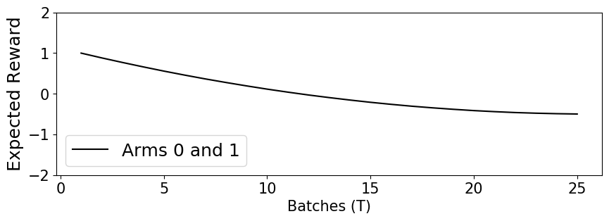
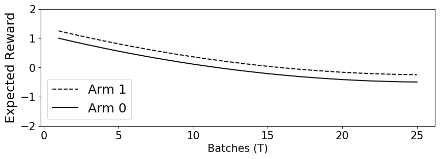
Many real-world problems we would like to use bandit algorithms for have non-stationary over time. For example, in online advertising, the effectiveness of an ad may change over time due to exposure to competing ads and general societal changes that could affect perceptions of an ad. We may believe that the expected reward for a given action may vary over time, but that the margin is constant from batch to batch. In the online advertising setting, this would mean whether one ad is always better than another is stable, but the overall effectiveness of both ads may change over time. In this case, we can simply use the BOLS test statistic described earlier in equation (4) to test $H_{0}\colon\Delta=0$ vs. $H_{1}\colon\Delta\neq 0$. Note that the BOLS test statistic for the margin is robust to non-stationarity in the baseline reward without any adjustment. Moreover, in our simulation settings we estimate the variance $\sigma^{2}$ separately for each batch, which allows for non-stationarity in the variance between batches as well; see Appendix A for variance estimation details and see Section 6 for simulation results. Additionally, in the case that we believe that the margin itself may vary from batch to batch, the BOLS test statistic can also be used to construct confidence regions that contain the true margin $\Delta_{t}$ for each batch simultaneously; see Appendix A.5 for details.

6 Simulation Experiments

Procedure

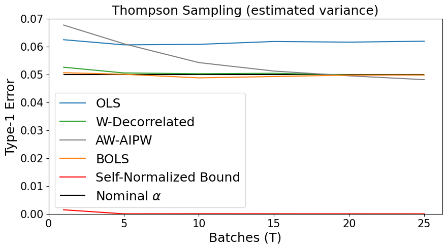
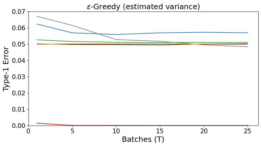
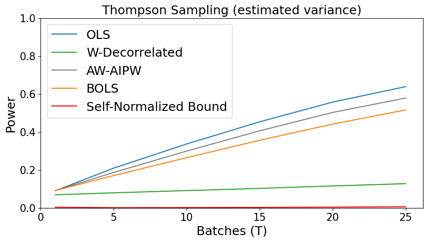
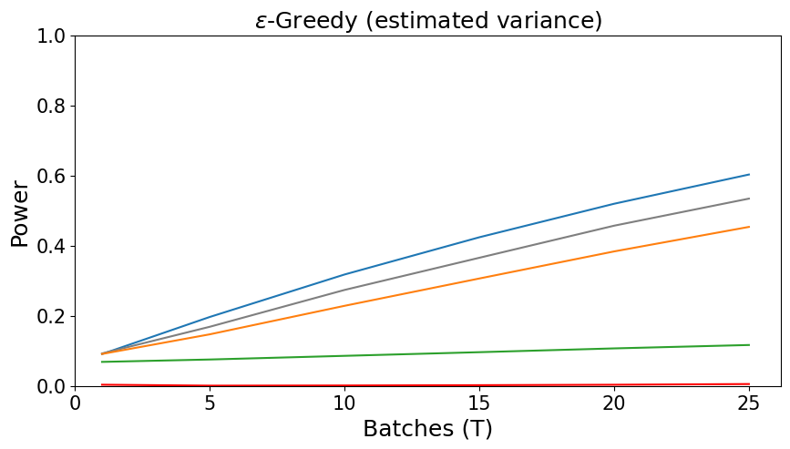
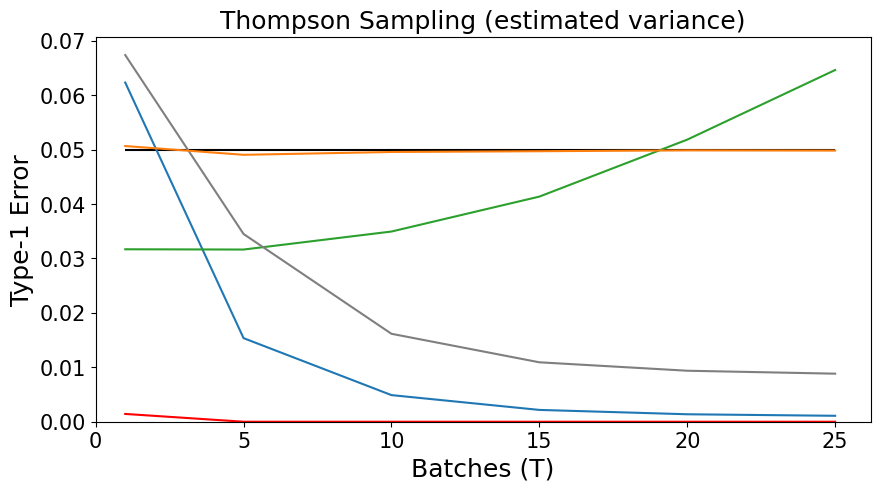
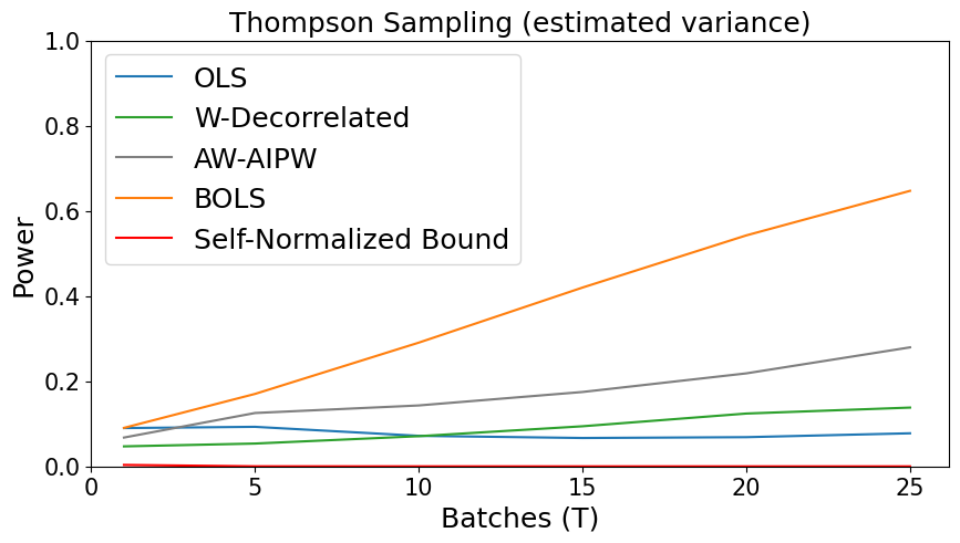
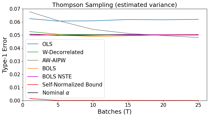
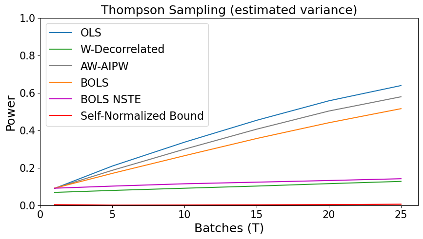
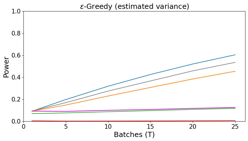
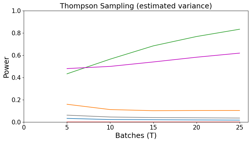
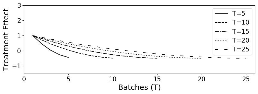
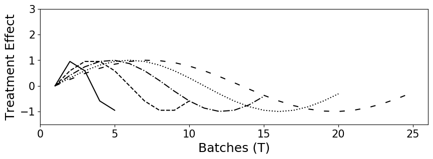
We focus on the two-arm bandit setting and test whether the margin is zero, specifically $H_{0}\colon\Delta=0$ vs. $H_{1}\colon\Delta\neq 0$. We perform experiments for when the noise variance $\sigma^{2}$ is estimated. We assume homoscedastic errors throughout. See Appendix A.4 for more details about how we estimate the noise variance and more details regarding our experimental setup. In Figures 6 and 7, we display results for stationary bandits and in Figure 5 we show results for bandits with non-stationary baseline rewards. See Appendix A.5 for results for bandits with non-stationary margins.

In our simulations, we found that OLS and AW-AIPW have inflated Type-1 error. Since Type-1 control is a hard constraint, solutions with inflated Type-1 error are infeasible solutions. In the power plots, we adjust the cutoffs of the estimators to ensure proper Type-1 error control; if an estimator has inflated Type-1 error under the null, in the power simulations we use a critical value estimated using the simulations under the null. Note that it is unfeasible to make these cutoff adjustment for real experiments (unless one found the worst case setting), as there are many nuisance parameters—like the expected rewards for each arm and the noise variance—which can affect cutoff values.

Results

Figure 3 shows that for small sample sizes ($nT\lesssim 300$), BOLS has more reliable Type-1 error control than AW-AIPW with variance stabilizing weights. After $nT\geq 500$ samples, AW-AIPW has proper Type-1 error, and by Figure 4 it always has slightly greater power than BOLS in the stationary setting. The W-decorrelated estimator has reliable Type-1 error control, but very low power compared to AW-AIPW and BOLS. Finally the high probability, self-normalized martingale bound of [1], which we use for hypothesis testing, has very low power compared to the asymptotic approximation statistical inference methods.

In Figure 5, we display simulation results for the non-stationary baseline reward setting. Whereas other estimators have no Type-1 error guarantees, BOLS still has proper Type-1 error control in the non-stationary baseline reward setting. Moreover, BOLS can have much greater power than other estimators when there is non-stationarity in the baseline reward. Overall, BOLS is favorable over other estimators in small-sample settings or when one wants to be robust to non-stationarity in the baseline reward—at the cost of losing a little power if the environment is stationary.

Figure 3: Stationary Setting: Type-1 error for a two-sided test of $H_{0}\colon\Delta=0$ vs. $H_{1}\colon\Delta\neq 0$ ($\alpha=0.05$). We set $\beta_{1}=\beta_{0}=0$, $n=25$, and a clipping constraint of $0.1\leq\pi_{t}^{(n)}\leq 0.9$. We use 100k Monte Carlo simulations and standard errors are $<0.001$.

Figure 4: Stationary Setting: Power for a two-sided test of $H_{0}\colon\Delta=0$ vs. $H_{1}\colon\Delta\neq 0$ ($\alpha=0.05$). We set $\beta_{1}=0$, $\beta_{0}=0.25$, $n=25$, and a clipping constraint of $0.1\leq\pi_{t}^{(n)}\leq 0.9$. We use 100k Monte Carlo simulations and standard errors are $<0.002$. We account for Type-1 error inflation as described in Section 6.

Figure 5: Non-stationary baseline reward setting: Type-1 error (upper left) and power (upper right) for a two-sided test of $H_{0}\colon\Delta=0$ vs. $H_{1}\colon\Delta\neq 0$ ($\alpha=0.05$). In the lower two plots we plot the expected rewards for each arm; note the margin is constant across batches. We use $n=25$ and a clipping constraint of $0.1\leq\pi_{t}^{(n)}\leq 0.9$. We use 100k Monte Carlo simulations and standard errors are $<0.002$.

7 Discussion

We found that the OLS estimator is asymptotically non-normal when the margin is zero due to the non-concentration of the action selection probabilities. Since the OLS estimator is a canonical example of a method-of-moments estimator [13], our results suggest that the inferential guarantees of standard method-of-moments estimators may fail to hold on adaptively collected data when there is no unique optimal, regret-minimizing policy. We develop the Batched OLS estimator, which is asymptotically normal even when the action selection probabilities do not concentrate. An open question is whether batched versions of general method-of-moments estimators could similarly be used for adaptive inference.

Broader Impact

Our work has the positive impact of encouraging the use of valid statistical inference methods on bandit data, which ultimately leads to more reliable scientific conclusions. In addition, by providing a valid statistical inference method on bandit data, our work facilitates the use of bandit algorithms in experimentation.

AAAA_batched_bandits_camera_ready

Appendix A Simulation Details

A.1 W-Decorrelated Estimator

For the $W$-decorrelated estimator [6], for a batch size of $n$ and for $T$ batches, we set $\lambda$ to be the $\frac{1}{nT}$ quantile of $\lambda_{\min}(\underline{\textbf{X}}^{\top}\underline{\textbf{X}})/\log(nT)$, where $\lambda_{\min}(\underline{\textbf{X}}^{\top}\underline{\textbf{X}})$ denotes the minimum eigenvalue of $\underline{\textbf{X}}^{\top}\underline{\textbf{X}}$. This procedure of choosing $\lambda$ is motivated by the conditions of Theorem 4 of [6] and follows the methods used by [6] in their simulation experiments. We had to adjust the original procedure for choosing $\lambda$ used by [6] (who set $\lambda$ to the $0.15$ quantile of $\lambda_{\min}(\underline{\textbf{X}}^{\top}\underline{\textbf{X}})$), because they only evaluated the W-decorrelated method for when the total number of samples was $nT=1000$ and valid values of $\lambda$ changes with the sample size.

A.2 AW-AIPW Estimator

Since the AW-AIPW test statistic for the treatment effect is not explicitly written in the original paper [11], we now write the formulas for the AW-AIPW estimator of the treatment effect: $\hat{\Delta}^{\textnormal{AW-AIPW}}:=\hat{\beta}_{1}^{\textnormal{AW-AIPW}}-\hat{\beta}_{0}^{\textnormal{AW-AIPW}}$. We use the variance stabilizing weights, equal to the square root of the sampling probabilities, $\sqrt{\pi_{t}^{(n)}}$ and $\sqrt{1-\pi_{t}^{(n)}}$. Below, $N_{t,1}=\sum_{i=1}^{n}A_{t,i}$ and $N_{t,0}=\sum_{i=1}^{n}(1-A_{t,i})$.

$$Y_{t,1}:=\frac{A_{t,i}}{\pi_{t}^{(n)}}R_{t,i}+\bigg{(}1-\frac{A_{t,i}^{(n)}}{\pi_{t}^{(n)}}\bigg{)}\frac{\sum_{t^{\prime}=1}^{t-1}\sum_{i=1}^{n}A_{t,i}^{(n)}R_{t,i}}{\sum_{t^{\prime}=1}^{t-1}N_{t^{\prime},1}}$$

$$Y_{t,0}:=\frac{1-A_{t,i}^{(n)}}{1-\pi_{t}^{(n)}}R_{t,i}+\bigg{(}1-\frac{1-A_{t,i}}{1-\pi_{t}^{(n)}}\bigg{)}\frac{\sum_{t^{\prime}=1}^{t-1}\sum_{i=1}^{n}(1-A_{t,i})R_{t,i}}{\sum_{t^{\prime}=1}^{t-1}N_{t^{\prime},0}}$$

$$\hat{\beta}_{1}^{\textnormal{AW-AIPW}}:=\frac{\sum_{t=1}^{T}\sum_{i=1}^{n}\sqrt{\pi_{t}^{(n)}}Y_{t,1}}{\sum_{t=1}^{T}\sum_{i=1}^{n}\sqrt{\pi_{t}^{(n)}}}~{}~{}~{}~{}\textnormal{ and }~{}~{}~{}~{}\hat{\beta}_{0}^{\textnormal{AW-AIPW}}:=\frac{\sum_{t=1}^{T}\sum_{i=1}^{n}\sqrt{1-\pi_{t}^{(n)}}Y_{t,0}}{\sum_{t=1}^{T}\sum_{i=1}^{n}\sqrt{1-\pi_{t}^{(n)}}}$$

The variance estimator for $\hat{\Delta}^{\textnormal{AW-AIPW}}$ is $\hat{V}_{0}+\hat{V}_{1}+2\hat{C}_{0,1}$ where

$$\hat{V}_{1}:=\frac{\sum_{t=1}^{T}\sum_{i=1}^{n}\pi_{t}^{(n)}(Y_{t,1}-\hat{\beta}_{1}^{\textnormal{AW-AIPW}})^{2}}{\bigg{(}\sum_{t=1}^{T}\sum_{i=1}^{n}\sqrt{\pi_{t}^{(n)}}\bigg{)}^{2}}~{}~{}~{}~{}\textnormal{ and }~{}~{}~{}~{}\hat{V}_{0}:=\frac{\sum_{t=1}^{T}\sum_{i=1}^{n}(1-\pi_{t}^{(n)})(Y_{t,0}-\hat{\beta}_{0}^{\textnormal{AW-AIPW}})^{2}}{\bigg{(}\sum_{t=1}^{T}\sum_{i=1}^{n}\sqrt{1-\pi_{t}^{(n)}}\bigg{)}^{2}}$$

$$\hat{C}_{0,1}:=-\frac{\sum_{t=1}^{T}\sum_{i=1}^{n}\sqrt{\pi_{t}^{(n)}(1-\pi_{t}^{(n)})}(Y_{t,1}-\hat{\beta}_{1}^{\textnormal{AW-AIPW}})(Y_{t,0}-\hat{\beta}_{0}^{\textnormal{AW-AIPW}})}{\bigg{(}\sum_{t=1}^{T}\sum_{i=1}^{n}\sqrt{\pi_{t}^{(n)}}\bigg{)}\bigg{(}\sum_{t=1}^{T}\sum_{i=1}^{n}\sqrt{1-\pi_{t}^{(n)}}\bigg{)}}$$

A.3 Self-Normalized Martingale Bound

By the self-normalized martingale bound of [1], specifically Theorem 1 and Lemma 6, we have that in the two arm bandit setting,

$$\mathbb{P}\left(\forall T,n\geq 1,\left|\hat{\beta}_{1}^{\textnormal{OLS}}-\beta_{1}\right|\leq c_{1,T}\textnormal{ and }\left|\hat{\beta}_{0}^{\textnormal{OLS}}-\beta_{0}\right|\leq c_{0,T}\right)\geq 1-\delta$$

where

$$c_{a,T}=\sqrt{\sigma^{2}\frac{1+\sum_{t=1}^{T}N_{t,a}}{\left(\sum_{t=1}^{T}N_{t,a}\right)^{2}}\left(1+2\log\left(\frac{2\sqrt{1+\sum_{t=1}^{T}N_{t,a}}}{\delta}\right)\right)}$$

We estimate $\sigma^{2}$ using the procedure stated below for the OLS estimator. We reject the null hypothesis that $\Delta=0$ whenever either the confidence bounds for the two arms are non-overlapping. Specifically when

$$\hat{\beta}_{1}^{\textnormal{OLS}}+c_{1,T}\leq\hat{\beta}_{0}^{\textnormal{OLS}}-c_{0,T}~{}~{}~{}\textnormal{ or }~{}~{}~{}\hat{\beta}_{0}^{\textnormal{OLS}}+c_{0,T}\leq\hat{\beta}_{1}^{\textnormal{OLS}}-c_{1,T}$$

A.4 Estimating Noise Variance

OLS Estimator

Given the OLS estimators for the means of each arm, $\hat{\beta}_{1}^{\textnormal{OLS}},\hat{\beta}_{0}^{\textnormal{OLS}}$, we estimate the noise variance $\sigma^{2}$ as follows:

$$\hat{\sigma}^{2}:=\frac{1}{nT-2}\sum_{t=1}^{T}\sum_{i=1}^{n}\bigg{(}R_{t,i}-A_{t,i}\hat{\beta}_{1}^{\textnormal{OLS}}-(1-A_{t,i})\hat{\beta}_{0}^{\textnormal{OLS}}\bigg{)}^{2}.$$

We use a degrees of freedom bias correction by normalizing by $nT-2$ rather than $nT$. Since the W-decorrelated estimator is a modified version of the OLS estimator, we also use this same noise variance estimator for the W-decorrelated estimator; we found that this worked well in practice, in terms of Type-1 error control.

Batched OLS

Given the Batched OLS estimators for the means of each arm for each batch, $\hat{\beta}_{t,1}^{\textnormal{BOLS}},\hat{\beta}_{t,0}^{\textnormal{BOLS}}$, we estimate the noise variance for each batch $\sigma_{t}^{2}$ as follows:

$$\hat{\sigma}_{t}^{2}:=\frac{1}{n-2}\sum_{i=1}^{n}\bigg{(}R_{t,i}-A_{t,i}\hat{\beta}_{t,1}^{\textnormal{BOLS}}-(1-A_{t,i})\hat{\beta}_{t,0}^{\textnormal{BOLS}}\bigg{)}^{2}.$$

Again, we use a degrees of freedom bias correction by normalizing by $n-2$ rather than $n$. We prove the consistency of $\hat{\sigma}_{t}^{2}$ (meaning $\hat{\sigma}_{t}^{2}\overset{P}{\to}\sigma^{2}$) in Corollary 4. Using BOLS to test $H_{0}:\Delta=a$ vs. $H_{1}:\Delta\neq a$, we use the following test statistic:

$$\frac{1}{\sqrt{T}}\sum_{t=1}^{T}\sqrt{\frac{N_{t,0}N_{t,1}}{n\hat{\sigma}_{t}^{2}}}(\hat{\Delta}_{t}^{\textnormal{BOLS}}-a).$$

Above, $N_{t,1}=\sum_{i=1}^{n}A_{t,i}$ and $N_{t,0}=\sum_{i=1}^{n}(1-A_{t,i})$. For this test statistic, we use cutoffs based on the Student-t distribution, i.e., for $Y_{t}\overset{i.i.d.}{\sim}t_{n-2}$ we use a cutoff $c_{\alpha/2}$ such that

$$\mathbb{P}\bigg{(}\bigg{|}\frac{1}{\sqrt{T}}\sum_{t=1}^{T}Y_{t}\bigg{|}>c_{\alpha/2}\bigg{)}=\alpha.$$

We found $c_{\alpha/2}$ by simulating draws from the Student-t distribution.

A.5 Non-Stationary Treatment Effect

When we believe that the margin itself varies from batch to batch, we are able to construct a confidence region that contains the true margin $\Delta_{t}$ for each batch simultaneously with probability $1-\alpha$.

Corollary 2 (Confidence band for margin for non-stationary bandits).

Assume the same conditions as Theorem 3. Let $z_{x}$ be $x^{\textnormal{th}}$ quantile of the standard Normal distribution, i.e., for $Z\sim\mathcal{N}(0,1)$, $\mathbb{P}(Z<z_{\alpha})=\alpha$. For each $t\in[1\colon T]$, we define the interval

$$\textbf{L}_{t}=\hat{\Delta}_{t}^{\textnormal{OLS}}\pm z_{1-\frac{\alpha}{2T}}\sqrt{\frac{\sigma^{2}n}{N_{t,0}N_{t,1}}}.$$

$\lim_{n\to\infty}\mathbb{P}\big{(}\forall t\in[1:T],\Delta_{t}\in\textbf{L}_{t}\big{)}\geq 1-\alpha$. Above, $N_{t,1}=\sum_{i=1}^{n}A_{t,i}$ and $N_{t,0}=\sum_{i=1}^{n}(1-A_{t,i})$.

Proof:

Note that by Corollary 3,

$$\mathbb{P}\big{(}\textnormal{exists some }t\in[1:T]~{}s.t.~{}\Delta_{t}\notin\textbf{L}_{t}\big{)}\leq\sum_{t=1}^{T}\mathbb{P}\big{(}\Delta_{t}\notin\textbf{L}_{t}\big{)}\to\sum_{t=1}^{T}\frac{\alpha}{T}=\alpha$$

where the limit is as $n\to\infty$. Since

$$\mathbb{P}\big{(}\forall t\in[1:T],\Delta_{t}\in\textbf{L}_{t}\big{)}=1-\mathbb{P}\big{(}\textnormal{exists some }t\in[1:T]~{}s.t.~{}\Delta_{t}\notin\textbf{L}_{t}\big{)}$$

Thus,

$$\lim_{n\to\infty}\mathbb{P}\big{(}\forall t\in[1:T],\Delta_{t}\in\textbf{L}_{t}\big{)}\geq 1-\alpha~{}~{}~{}\qed$$

We can also test the null hypothesis of no margin against the alternative that at least one batch has non-zero margin, i.e., $H_{0}\colon\forall t\in[1\colon T],\Delta_{t}=0$ vs. $H_{1}\colon\exists t\in[1\colon T]~{}s.t.~{}\Delta_{t}\not=0$. Note that the global null stated above is of great interest in the mobile health literature [23, 30]. Specifically we use the following test statistic:

$$\sum_{t=1}^{T}\frac{N_{t,0}N_{t,1}}{\sigma^{2}n}(\hat{\Delta}_{t}^{\textnormal{OLS}}-0)^{2},$$

which by Theorem 3 converges in distribution to a chi-squared distribution with $T$ degrees of freedom under the null $\Delta_{t}=0$ for all $t$.

To account for estimating noise variance $\sigma^{2}$, in our simulations for this test statistic, we use cutoffs based on the Student-t distribution, i.e., for $Y_{t}\overset{i.i.d.}{\sim}t_{n-2}$ we use a cutoff $c_{\alpha/2}$ such that

$$\mathbb{P}\bigg{(}\frac{1}{T}\sum_{t=1}^{T}Y_{t}^{2}>c_{\alpha}\bigg{)}=\alpha.$$

We found $c_{\alpha}$ by simulating draws from the Student-t distribution.

In the plots below we call the test statistic in (A.5) “BOLS Non-Stationary Treatment Effect” (BOLS NSTE). BOLS NSTE performs poorly in terms of power compared to other test statistics in the stationary setting; however, in the non-stationary setting, BOLS NSTE significantly outperforms all other test statistics, which tend to have low power when the average treatment effect is close to zero. Note that the W-decorrelated estimator performs well in the left plot of Figure 8; this is because as we show in Appendix F, the W-decorrelated estimator upweights samples from the earlier batches in the study. So when the treatment effect is large in the beginning of the study, the W-decorrelated estimator has high power and when the treatment effect is small or zero in the beginning of the study, the W-decorrelated estimator has low power.

Figure 6: Stationary Setting: Type-1 error for a two-sided test of $H_{0}\colon\Delta=0$ vs. $H_{1}\colon\Delta\neq 0$ ($\alpha=0.05$). We set $\beta_{1}=\beta_{0}=0$, $n=25$, and a clipping constraint of $0.1\leq\pi_{t}^{(n)}\leq 0.9$. We use 100k Monte Carlo simulations and standard errors are $<0.001$.

Figure 7: Stationary Setting: Power for a two-sided test of $H_{0}\colon\Delta=0$ vs. $H_{1}\colon\Delta\neq 0$ ($\alpha=0.05$). We set $\beta_{1}=0$, $\beta_{0}=0.25$, $n=25$, and a clipping constraint of $0.1\leq\pi_{t}^{(n)}\leq 0.9$. We use 100k Monte Carlo simulations and standard errors are $<0.002$. We account for Type-1 error inflation as described in Section 6.

Figure 8: Nonstationary setting: The two upper plots display the power of estimators for a two-sided test of $H_{0}\colon\forall t\in[1\colon T],~{}\beta_{t,1}-\beta_{t,0}=0$ vs. $H_{1}\colon\exists t\in[1\colon T],\beta_{t,1}-\beta_{t,0}\neq 0$ ($\alpha=0.05$). The two lower plots display two treatment effect trends; the left plot considers a decreasing trend (quadratic function) and the right plot considers a oscillating trend ($\sin$ function). We set $n=25$, and a clipping constraint of $0.1\leq\pi_{t}^{(n)}\leq 0.9$. We use 100k Monte Carlo simulations and standard errors are $<0.002$.

AAAA_batched_bandits_camera_ready AAAA_batched_bandits_camera_ready

Appendix B Asymptotic Normality of the OLS Estimator

Condition 6 (Weak moments).

$\forall t,n,i$, $\mathbb{E}[\epsilon_{t,i}^{2}\big{|}\mathcal{G}_{t-1}^{(n)}]=\sigma^{2}$ and for all $\forall t,n,i$, $\mathbb{E}[\varphi(\epsilon_{t,i}^{2})|\mathcal{G}_{t-1}^{(n)}]<M<\infty$ a.s. for some function $\varphi$ where $\lim_{x\to\infty}\frac{\varphi(x)}{x}\to\infty$.

Condition 7 (Stability).

There exists a sequence of nonrandom positive-definite symmetric matrices, $\underline{\textbf{V}}_{n}$, such that

1. $\underline{\textbf{V}}_{n}^{-1}\big{(}\sum_{t=1}^{T}\sum_{i=1}^{n}\textbf{X}_{t,i}\textbf{X}_{t,i}^{\top}\big{)}^{\frac{1}{2}}=\underline{\textbf{V}}_{n}^{-1}\big{(}\underline{\textbf{X}}^{\top}\underline{\textbf{X}}\big{)}^{\frac{1}{2}}\overset{P}{\to}\underline{\textbf{I}}_{p}$

2. $\max_{i\in[1\colon n],t\in[1\colon T]}\|\underline{\textbf{V}}_{n}^{-1}\textbf{X}_{t,i}\|_{2}\overset{P}{\to}0$

Theorem 5 (Triangular array version of Lai & Wei (1982), Theorem 3).

Let $\textbf{X}_{t,i}\in^{p}$ be non-anticipating with respect to filtration $\{\mathcal{G}_{t}^{(n)}\}_{t=1}^{T}$, so $\textbf{X}_{t,i}$ is $\mathcal{G}_{t-1}^{(n)}$ measurable. We assume the following conditional mean model for rewards:

$$\mathbb{E}\big{[}R_{t,i}\big{|}\mathcal{G}_{t-1}^{(n)}\big{]}=\textbf{X}_{t,i}^{\top}\boldsymbol{\beta}.$$

We define $\epsilon_{t,i}:=R_{t,i}-\textbf{X}_{t,i}^{\top}\boldsymbol{\beta}$. Note that $\{\epsilon_{t,i}\}_{i=1,t=1}^{i=n,t=T}$ is a martingale difference array with respect to filtration $\{\mathcal{G}_{t}^{(n)}\}_{t=1}^{T}$.

Assuming Conditions 6 and 7, as $n\to\infty$,

$$(\underline{\textbf{X}}^{\top}\underline{\textbf{X}})^{1/2}(\boldsymbol{\hat{\beta}}^{\textnormal{OLS}}-\boldsymbol{\beta})\overset{D}{\to}\mathcal{N}(0,\sigma^{2}\underline{\textbf{I}}_{p})$$

Note, in the body of the paper we state that this theorem holds in the two-arm bandit case assuming Conditions 2 and 1. Note that Condition 1 is sufficient for Condition 6 and Condition 2 is sufficient for Condition 7 in the two-arm bandit case.

Proof:

$$\boldsymbol{\hat{\beta}}^{\textnormal{OLS}}=((\underline{\textbf{X}}^{\top}\underline{\textbf{X}})^{-1}\underline{\textbf{X}}^{(n),\top}\textbf{R}^{(n)}=(\underline{\textbf{X}}^{\top}\underline{\textbf{X}})^{-1}\underline{\textbf{X}}^{\top}(\underline{\textbf{X}}\boldsymbol{\beta}+\boldsymbol{\epsilon})$$

$$\boldsymbol{\hat{\beta}}^{\textnormal{OLS}}-\boldsymbol{\beta}=(\underline{\textbf{X}}^{\top}\underline{\textbf{X}})^{-1}\underline{\textbf{X}}^{\top}\boldsymbol{\epsilon}=\bigg{(}\sum_{t=1}^{T}\sum_{i=1}^{n}\textbf{X}_{t,i}\textbf{X}_{t,i}^{\top}\bigg{)}^{-1}\sum_{t=1}^{T}\sum_{i=1}^{n}\textbf{X}_{t,i}\epsilon_{t,i}$$

It is sufficient to show that as $n\to\infty$:

$$(\underline{\textbf{X}}^{\top}\underline{\textbf{X}})^{-1/2}\sum_{t=1}^{T}\sum_{i=1}^{n}\textbf{X}_{t,i}\epsilon_{t,i}\overset{D}{\to}\mathcal{N}(0,\sigma^{2}\underline{\textbf{I}}_{p})$$

By Slutsky’s Theorem and Condition 7 (a), it is also sufficient to show that as $n\to\infty$,

$$\underline{\textbf{V}}_{n}^{-1}\sum_{t=1}^{T}\sum_{i=1}^{n}\textbf{X}_{t,i}\epsilon_{t,i}\overset{D}{\to}\mathcal{N}(0,\sigma^{2}\underline{\textbf{I}}_{p})$$

By Cramer-Wold device, it is sufficient to show multivariate normality if for any fixed $\textbf{c}\in^{p}$ s.t. $\|\textbf{c}\|_{2}=1$, as $n\to\infty$,

$$\textbf{c}^{\top}\underline{\textbf{V}}_{n}^{-1}\sum_{t=1}^{T}\sum_{i=1}^{n}\textbf{X}_{t,i}\epsilon_{t,i}\overset{D}{\to}\mathcal{N}(0,\sigma^{2})$$

We will prove this central limit theorem by using a triangular array martingale central limit theorem, specifically Theorem 2.2 of [8]. We will do this by letting $Y_{t,i}=\textbf{c}^{T}\underline{\textbf{V}}_{n}^{-1}\textbf{X}_{t,i}\epsilon_{t,i}$. The theorem states that as $n\to\infty$, $\sum_{t=1}^{T}\sum_{i=1}^{n}Y_{t,i}\overset{D}{\to}\mathcal{N}(0,\sigma^{2})$ if the following conditions hold as $n\to\infty$:

1. $\sum_{t=1}^{T}\sum_{i=1}^{n}E[Y_{t,i}|\mathcal{G}_{t-1}^{(n)}]\overset{P}{\to}0$

2. $\sum_{t=1}^{T}\sum_{i=1}^{n}E[Y_{t,i}^{2}|\mathcal{G}_{t-1}^{(n)}]\overset{P}{\to}\sigma^{2}$

3. $\forall\delta>0,\sum_{t=1}^{T}\sum_{i=1}^{n}E\big{[}Y_{t,i}^{2}\mathbb{I}_{(|Y_{t,i}|>\delta)}\big{|}\mathcal{G}_{t-1}^{(n)}\big{]}\overset{P}{\to}0$

Useful Properties

Note that by Cauchy-Schwartz and Condition 7 (b), as $n\to\infty$,

$$\max_{i\in[1\colon n],t\in[1\colon T]}\big{|}\textbf{c}^{\top}\underline{\textbf{V}}_{n}^{-1}\textbf{X}_{t,i}\big{|}\leq\max_{i\in[1\colon n],t\in[1\colon T]}\|\textbf{c}\|_{2}\|\underline{\textbf{V}}_{n}^{-1}\textbf{X}_{t,i}\|_{2}\overset{P}{\to}0$$

By continuous mapping theorem and since the square function on non-negative inputs is order preserving, as $n\to\infty$,

$$\bigg{(}\max_{i\in[1\colon n],t\in[1\colon T]}\big{|}\textbf{c}^{\top}\underline{\textbf{V}}_{n}^{-1}\textbf{X}_{t,i}\big{|}\bigg{)}^{2}=\max_{i\in[1\colon n],t\in[1\colon T]}\big{(}\textbf{c}^{\top}\underline{\textbf{V}}_{n}^{-1}\textbf{X}_{t,i}\big{)}^{2}\overset{P}{\to}0$$ (5)

By Condition 7 (a) and continuous mapping theorem, $\textbf{c}^{\top}\underline{\textbf{V}}_{n}^{-1}(\textbf{X}_{t,i}^{\top}\textbf{X}_{t,i})^{1/2}\overset{P}{\to}\textbf{c}^{\top}$, so

$$\textbf{c}^{\top}\underline{\textbf{V}}_{n}^{-1}(\textbf{X}_{t,i}^{\top}\textbf{X}_{t,i})^{1/2}(\textbf{X}_{t,i}^{\top}\textbf{X}_{t,i})^{1/2}\underline{\textbf{V}}_{n}^{-1}\textbf{c}\overset{P}{\to}\textbf{c}^{\top}\textbf{c}=1$$

Thus,

$$\textbf{c}^{\top}\underline{\textbf{V}}_{n}^{-1}\bigg{(}\sum_{t=1}^{T}\sum_{i=1}^{n}\textbf{X}_{t,i}\textbf{X}_{t,i}^{\top}\bigg{)}\underline{\textbf{V}}_{n}^{-1}\textbf{c}=\sum_{t=1}^{T}\sum_{i=1}^{n}\textbf{c}^{\top}\underline{\textbf{V}}_{n}^{-1}\textbf{X}_{t,i}\textbf{X}_{t,i}^{\top}\underline{\textbf{V}}_{n}^{-1}\textbf{c}\overset{P}{\to}1$$

Since $\textbf{c}^{\top}\underline{\textbf{V}}_{n}^{-1}\textbf{X}_{t,i}$ is a scalar, as $n\to\infty$,

$$\sum_{t=1}^{T}\sum_{i=1}^{n}(\textbf{c}^{\top}\underline{\textbf{V}}_{n}^{-1}\textbf{X}_{t,i})^{2}\overset{P}{\to}1$$ (6)

Condition (a): Martingale

$$\sum_{t=1}^{T}\sum_{i=1}^{n}\mathbb{E}[\textbf{c}^{\top}\underline{\textbf{V}}_{n}^{-1}\textbf{X}_{t,i}\epsilon_{t,i}|\mathcal{G}_{t-1}^{(n)}]=\sum_{t=1}^{T}\sum_{i=1}^{n}\textbf{c}^{\top}\underline{\textbf{V}}_{n}^{-1}\textbf{X}_{t,i}\mathbb{E}[\epsilon_{t,i}|\mathcal{G}_{t-1}^{(n)}]=0$$

Condition (b): Conditional Variance

$$\sum_{t=1}^{T}\sum_{i=1}^{n}\mathbb{E}[(\textbf{c}^{\top}\underline{\textbf{V}}_{n}^{-1}\textbf{X}_{t,i})^{2}\epsilon_{t,i}^{2}|\mathcal{G}_{t-1}^{(n)}]=\sum_{t=1}^{T}\sum_{i=1}^{n}(\textbf{c}^{\top}\underline{\textbf{V}}_{n}^{-1}\textbf{X}_{t,i})^{2}\mathbb{E}[\epsilon_{t,i}^{2}|\mathcal{G}_{t-1}^{(n)}]=\sigma^{2}\sum_{t=1}^{T}\sum_{i=1}^{n}(\textbf{c}^{\top}\underline{\textbf{V}}_{n}^{-1}\textbf{X}_{t,i})^{2}\overset{P}{\to}\sigma^{2}$$

where the last equality holds by Condition 6 and the limit holds by (6) as $n\to\infty$.

Condition (c): Lindeberg Condition

Let $\delta>0$. We want to show that as $n\to\infty$,

$$\sum_{t=1}^{T}\sum_{i=1}^{n}Z_{t,i}^{2}\mathbb{E}\bigg{[}\epsilon_{t,i}^{2}\mathbb{I}_{(Z_{t,i}^{2}\epsilon_{t,i}^{2}>\delta^{2})}\bigg{|}\mathcal{G}_{t-1}^{(n)}\bigg{]}\overset{P}{\to}0$$

where above, we define $Z_{t,i}^{(n)}:=\textbf{c}^{\top}\underline{\textbf{V}}_{n}^{-1}\textbf{X}_{t,i}$. By Condition 6, we have that for all $n\geq 1$,

$$\max_{t\in[1\colon T],i\in[1\colon n]}\mathbb{E}[\varphi(\epsilon_{t,i}^{2})|\mathcal{G}_{t-1}^{(n)}]<M$$

Since we assume that $\lim_{x\to\infty}\frac{\varphi(x)}{x}=\infty$, for all $m\geq 1$, there exists a $b_{m}$ s.t. $\varphi(x)\geq mMx$ for all $x\geq b_{m}$. So, for all $n,t,i$,

$$M\geq\mathbb{E}[\varphi(\epsilon_{t,i}^{2})|\mathcal{G}_{t-1}^{(n)}]\geq\mathbb{E}[\varphi(\epsilon_{t,i}^{2})\mathbb{I}_{(\epsilon_{t,i}^{2}\geq b_{m})}|\mathcal{G}_{t-1}^{(n)}]\geq mM\mathbb{E}[\epsilon_{t,i}^{2}\mathbb{I}_{(\epsilon_{t,i}^{2}\geq b_{m})}|\mathcal{G}_{t-1}^{(n)}]$$

Thus,

$$\max_{t\in[1\colon T],i\in[1\colon n]}\mathbb{E}[\epsilon_{t,i}^{2}\mathbb{I}_{(\epsilon_{t,i}^{2}\geq b_{m})}|\mathcal{G}_{t-1}^{(n)}]\leq\frac{1}{m}$$

So we have that

$$\sum_{t=1}^{T}\sum_{i=1}^{n}Z_{t,i}^{2}\mathbb{E}\big{[}\epsilon_{t,i}^{2}\mathbb{I}_{(Z_{t,i}^{2}\epsilon_{t,i}^{2}>\delta^{2})}\big{|}\mathcal{G}_{t-1}^{(n)}\big{]}$$

$$=\sum_{t=1}^{T}\sum_{i=1}^{n}Z_{t,i}^{2}\bigg{(}\mathbb{E}\bigg{[}\epsilon_{t,i}^{2}\mathbb{I}_{(Z_{t,i}^{2}\epsilon_{t,i}^{2}>\delta^{2})}\bigg{|}\mathcal{G}_{t-1}^{(n)}\bigg{]}\mathbb{I}_{(Z_{t,i}^{2}\leq\delta^{2}/b_{m})}+\mathbb{E}\bigg{[}\epsilon_{t,i}^{2}\mathbb{I}_{(Z_{t,i}^{2}\epsilon_{t,i}^{2}>\delta^{2})}\bigg{|}\mathcal{G}_{t-1}^{(n)}\bigg{]}\mathbb{I}_{(Z_{t,i}^{2}>\delta^{2}/b_{m})}\bigg{)}$$

$$\leq\sum_{t=1}^{T}\sum_{i=1}^{n}Z_{t,i}^{2}\bigg{(}\mathbb{E}\bigg{[}\epsilon_{t,i}^{2}\mathbb{I}_{(\epsilon_{t,i}^{2}>b_{m})}\bigg{|}\mathcal{G}_{t-1}^{(n)}\bigg{]}+\sigma^{2}\mathbb{I}_{(Z_{t,i}^{2}>\delta^{2}/b_{m})}\bigg{)}$$

$$\leq\bigg{(}\frac{1}{m}+\sigma^{2}\mathbb{I}_{(\max_{t^{\prime}\in[1\colon T],j\in[1\colon n]}Z_{t^{\prime},j}^{2}>\delta^{2}/b_{m})}\bigg{)}\sum_{t=1}^{T}\sum_{i=1}^{n}Z_{t,i}^{2}$$

By Slutsky’s Theorem and (6), it is sufficient to show that as $n\to\infty$,

$$\frac{1}{m}+\sigma^{2}\mathbb{I}_{(\max_{t^{\prime}\in[1\colon T],j\in[1\colon n]}Z_{t^{\prime},j}^{2}>\delta^{2}/b_{m})}\overset{P}{\to}0$$

For any $\epsilon>0$,

$$\mathbb{P}\bigg{(}\frac{1}{m}+\sigma^{2}\mathbb{I}_{(\max_{t^{\prime}\in[1\colon T],j\in[1\colon n]}Z_{t^{\prime},j}^{2}>\delta^{2}/b_{m})}>\epsilon\bigg{)}\leq\mathbb{I}_{(\frac{1}{m}>\frac{\epsilon}{2})}+\mathbb{P}\bigg{(}\sigma^{2}\mathbb{I}_{(\max_{t^{\prime}\in[1\colon T],j\in[1\colon n]}Z_{t^{\prime},j}^{2}>\delta^{2}/b_{m})}>\frac{\epsilon}{2}\bigg{)}$$

We can choose $m$ such that $\frac{1}{m}\leq\frac{\epsilon}{2}$, so $\mathbb{P}\big{(}\frac{1}{m}>\frac{\epsilon}{2}\big{)}=0$. For the second term (note that $m$ is now fixed),

$$\mathbb{P}\bigg{(}\sigma^{2}\mathbb{I}_{(\max_{t^{\prime}\in[1\colon T],j\in[1\colon n]}Z_{t^{\prime},j}^{2}>\delta^{2}/b_{m})}>\frac{\epsilon}{2}\bigg{)}\leq\mathbb{P}\bigg{(}\max_{t^{\prime}\in[1\colon T],j\in[1\colon n]}Z_{t^{\prime},j}^{2}>\delta^{2}/b_{m}\bigg{)}\to 0$$

where the last limit holds by (5) as $n\to\infty$. ∎

B.1 Corollary 1 (Sufficient conditions for Theorem 5)

Under Conditions 1 and 3, when the treatment effect is non-zero data collected in batches using $\epsilon$-greedy, Thompson Sampling, or UCB with a fixed clipping constraint (see Definition 1) will satisfy Theorem 5 conditions.

Proof:

The only condition of Theorem 5 that needs to verified is Condition 2. To satisfy Condition 2, it is sufficient to show that for any given $\Delta$, for some constant $c\in(0,T)$,

$$\frac{1}{n}\sum_{t=1}^{T}\sum_{i=1}^{n}A_{t,i}=\frac{1}{n}\sum_{t=1}^{T}N_{t,1}\overset{P}{\to}c.$$

$\epsilon$-greedy We assume without loss of generality that $\Delta>0$ and $\pi_{1}^{(n)}=\frac{1}{2}$. Recall that for $\epsilon$-greedy, for $a\in[2\colon T]$,

$$\pi_{a}^{(n)}=\begin{cases}1-\frac{\epsilon}{2}&\textnormal{ if }\frac{\sum_{t=1}^{a}\sum_{i=1}^{n}A_{t,i}R_{t,i}}{\sum_{t^{\prime}=1}^{a}N_{t^{\prime},1}}>\frac{\sum_{t=1}^{a}\sum_{i=1}^{n}(1-A_{t,i})R_{t,i}}{\sum_{t^{\prime}=1}^{a}N_{t^{\prime},0}}\\ \frac{\epsilon}{2}&\textnormal{ otherwise }\end{cases}$$

Thus to show that $\pi_{a}^{(n)}\overset{P}{\to}1-\frac{\epsilon}{2}$ for all $a\in[2\colon T]$, it is sufficient to show that

$$\mathbb{P}\bigg{(}\frac{\sum_{t=1}^{a}\sum_{i=1}^{n}A_{t,i}R_{t,i}}{\sum_{t^{\prime}=1}^{a}N_{t^{\prime},1}}>\frac{\sum_{t=1}^{a}\sum_{i=1}^{n}(1-A_{t,i})R_{t,i}}{\sum_{t^{\prime}=1}^{a}N_{t^{\prime},0}}\bigg{)}\to 1$$ (7)

To show (7), it is equivalent to show that

$$\mathbb{P}\bigg{(}\Delta>\frac{\sum_{t=1}^{a}\sum_{i=1}^{n}(1-A_{t,i})\epsilon_{t,i}}{\sum_{t^{\prime}=1}^{a}N_{t^{\prime},0}}-\frac{\sum_{t=1}^{a}\sum_{i=1}^{n}A_{t,i}\epsilon_{t,i}}{\sum_{t^{\prime}=1}^{a}N_{t^{\prime},1}}\bigg{)}\to 1$$ (8)

To show (8), it is sufficient to show that

$$\frac{\sum_{t=1}^{a}\sum_{i=1}^{n}(1-A_{t,i})\epsilon_{t,i}}{\sum_{t^{\prime}=1}^{a}N_{t^{\prime},0}}-\frac{\sum_{t=1}^{a}\sum_{i=1}^{n}A_{t,i}\epsilon_{t,i}}{\sum_{t^{\prime}=1}^{a}N_{t^{\prime},1}}\overset{P}{\to}0.$$ (9)

To show (9), it is equivalent to show that

$$\sum_{t=1}^{a}\frac{\sqrt{N_{t,0}}}{\sum_{t^{\prime}=1}^{a}N_{t^{\prime},0}}\frac{\sum_{i=1}^{n}(1-A_{t,i})\epsilon_{t,i}}{\sqrt{N_{t,0}}}-\sum_{t=1}^{a}\frac{\sqrt{N_{t,1}}}{\sum_{t^{\prime}=1}^{a}N_{t^{\prime},1}}\frac{\sum_{i=1}^{n}A_{t,i}\epsilon_{t,i}}{\sqrt{N_{t,1}}}\overset{P}{\to}0.$$ (10)

By Lemma 1, for all $t\in[1\colon T]$,

$$\frac{N_{t,1}}{\pi_{t}^{(n)}n}\overset{P}{\to}1$$

Thus by Slutsky’s Theorem, to show (10), it is sufficient to show that

$$\sum_{t=1}^{a}\frac{\sqrt{n(1-\pi_{t}^{(n)})}}{n\sum_{t^{\prime}=1}^{a}(1-\pi_{t^{\prime}}^{(n)})}\frac{\sum_{i=1}^{n}(1-A_{t,i})\epsilon_{t,i}}{\sqrt{N_{t,0}}}-\sum_{t=1}^{a}\frac{\sqrt{n\pi_{t}^{(n)}}}{n\sum_{t^{\prime}=1}^{a}\pi_{t^{\prime}}^{(n)}}\frac{\sum_{i=1}^{n}A_{t,i}\epsilon_{t,i}}{\sqrt{N_{t,1}}}\overset{P}{\to}0.$$ (11)

Since $\pi_{t}^{(n)}\in[\frac{\epsilon}{2},1-\frac{\epsilon}{2}]$ for all $t,n$, the left hand side of (11) equals the following:

$$\sum_{t=1}^{a}o_{p}(1)\frac{\sum_{i=1}^{n}(1-A_{t,i})\epsilon_{t,i}}{\sqrt{N_{t,0}}}-\sum_{t=1}^{a}o_{p}(1)\frac{\sum_{i=1}^{n}A_{t,i}\epsilon_{t,i}}{\sqrt{N_{t,1}}}\overset{P}{\to}0.$$

The above limit holds because by Thereom 3, we have that

$$\bigg{(}\frac{\sum_{i=1}^{n}A_{1,i}\epsilon_{1,i}}{\sqrt{N_{1,1}}},\frac{\sum_{i=1}^{n}(1-A_{1,i})\epsilon_{1,i}}{\sqrt{N_{1,0}}},...,\frac{\sum_{i=1}^{n}A_{T,i}\epsilon_{T,i}}{\sqrt{N_{T,1}}},\frac{\sum_{i=1}^{n}(1-A_{T,i})\epsilon_{T,i}}{\sqrt{N_{T,0}}}\bigg{)}\overset{D}{\to}\mathcal{N}(\boldsymbol{0},\sigma^{2}\underline{\boldsymbol{I}}_{2T}).$$ (12)

Thus, by Slutsky’s Theorem and Lemma 1, we have that

$$\frac{1}{n}\sum_{t=1}^{T}N_{t,1}\overset{P}{\to}\frac{1}{2}+(T-1)(1-\frac{\epsilon}{2})~{}~{}~{}~{}~{}~{}~{}~{}~{}\textnormal{ and }~{}~{}~{}~{}~{}~{}~{}~{}~{}~{}\frac{1}{n}\sum_{t=1}^{T}N_{t,0}\overset{P}{\to}\frac{1}{2}+(T-1)\frac{\epsilon}{2}$$

Thompson Sampling We assume without loss of generality that $\Delta>0$ and $\pi_{1}^{(n)}=\frac{1}{2}$. Recall that for Thompson Sampling with independent standard normal priors ($\tilde{\beta}_{1},\tilde{\beta}_{0}\overset{i.i.d.}{\sim}\mathcal{N}(0,1)$) for $a\in[2\colon T]$,

$$\pi_{a}^{(n)}=\pi_{\min}\vee\big{[}\pi_{\max}\wedge\mathbb{P}(\tilde{\beta}_{1}>\tilde{\beta}_{0}~{}|~{}H_{a-1}^{(n)})\big{]}$$

Given the independent standard normal priors on $\tilde{\beta}_{1},\tilde{\beta}_{0}$, we have the following posterior distribution:

$$\tilde{\beta}_{1}-\tilde{\beta}_{0}~{}|~{}H_{a-1}^{(n)}\sim\mathcal{N}\bigg{(}\frac{\sum_{t=1}^{a-1}\sum_{i=1}^{n}A_{t,i}R_{t,i}}{\sigma^{2}+\sum_{t=1}^{a-1}N_{t,1}}-\frac{\sum_{t=1}^{a-1}\sum_{i=1}^{n}(1-A_{t,i})R_{t,i}}{\sigma^{2}+\sum_{t=1}^{a-1}N_{t,0}},\\ \frac{\sigma^{2}(\sigma^{2}+\sum_{t=1}^{a-1}N_{t,1})+\sigma^{2}(\sigma^{2}+\sum_{t=1}^{a-1}N_{t,0})}{(\sigma^{2}+\sum_{t=1}^{a-1}N_{t,0})(\sigma^{2}+\sum_{t=1}^{a-1}N_{t,1})}\bigg{)}$$

$$=:\mathcal{N}\big{(}\mu_{a-1}^{(n)},(\sigma_{a-1}^{(n)})^{2}\big{)}$$

Thus to show that $\pi_{a}^{(n)}\overset{P}{\to}\pi_{\max}$ for all $a\in[2\colon T]$, it is sufficient to show that $\mu_{a-1}^{(n)}\overset{P}{\to}\Delta$ and $(\sigma_{a-1}^{(n)})^{2}\overset{P}{\to}0$ for all $a\in[2\colon T]$. By Lemma 1, for all $t\in[1\colon T]$,

$$\frac{N_{t,1}}{\pi_{t}^{(n)}n}\overset{P}{\to}1$$

Thus, to show $(\sigma_{a-1}^{(n)})^{2}\overset{P}{\to}0$, it is sufficient to show that

$$\frac{\sigma^{2}(\sigma^{2}+n\sum_{t=1}^{a-1}\pi_{t}^{(n)})+\sigma^{2}(\sigma^{2}+n\sum_{t=1}^{a-1}(1-\pi_{t}^{(n)}))}{(\sigma^{2}+n\sum_{t=1}^{a-1}(1-\pi_{t}^{(n)}))(\sigma^{2}+n\sum_{t=1}^{a-1}\pi_{t}^{(n)})}\overset{P}{\to}0$$

The above limit holds because $\pi_{t}^{(n)}\in[\pi_{\min},\pi_{\max}]$ for $0<\pi_{\min}\leq\pi_{\max}<1$ by the clipping condition.

We now show that $\mu_{a-1}^{(n)}\overset{P}{\to}\Delta$, which is equivalent to showing that the following converges in probability to $\Delta$

$$\frac{\sum_{t=1}^{a-1}\sum_{i=1}^{n}A_{t,i}R_{t,i}}{\sigma^{2}+\sum_{t=1}^{a-1}N_{t,1}}-\frac{\sum_{t=1}^{a-1}\sum_{i=1}^{n}(1-A_{t,i})R_{t,i}}{\sigma^{2}+\sum_{t=1}^{a-1}N_{t,0}}$$

$$=\frac{\sum_{t=1}^{a-1}N_{t,1}}{\sigma^{2}+\sum_{t=1}^{a-1}N_{t,1}}\frac{\sum_{t=1}^{a-1}\sum_{i=1}^{n}A_{t,i}R_{t,i}}{\sum_{t=1}^{a-1}N_{t,1}}-\frac{\sum_{t=1}^{a-1}N_{t,0}}{\sigma^{2}+\sum_{t=1}^{a-1}N_{t,0}}\frac{\sum_{t=1}^{a-1}\sum_{i=1}^{n}(1-A_{t,i})R_{t,i}}{\sum_{t=1}^{a-1}N_{t,0}}$$

$$=\frac{\sum_{t=1}^{a-1}N_{t,1}}{\sigma^{2}+\sum_{t=1}^{a-1}N_{t,1}}\bigg{(}\beta_{1}+\frac{\sum_{t=1}^{a-1}\sum_{i=1}^{n}A_{t,i}\epsilon_{t,i}}{\sum_{t=1}^{a-1}N_{t,1}}\bigg{)}\\ -\frac{\sum_{t=1}^{a-1}N_{t,0}}{\sigma^{2}+\sum_{t=1}^{a-1}N_{t,0}}\bigg{(}\beta_{0}+\frac{\sum_{t=1}^{a-1}\sum_{i=1}^{n}(1-A_{t,i})\epsilon_{t,i}}{\sum_{t=1}^{a-1}N_{t,0}}\bigg{)}$$ (13)

Note that

$$\frac{\sum_{t=1}^{a-1}N_{t,1}}{\sigma^{2}+\sum_{t=1}^{a-1}N_{t,1}}\beta_{1}-\frac{\sum_{t=1}^{a-1}N_{t,0}}{\sigma^{2}+\sum_{t=1}^{a-1}N_{t,0}}\beta_{0}\overset{P}{\to}\Delta$$ (14)

Equation (14) above holds by Lemma 1, because

$$\frac{n\sum_{t=1}^{a-1}\pi_{t}^{(n)}}{\sigma^{2}+n\sum_{t=1}^{a-1}\pi_{t}^{(n)}}\overset{P}{\to}1~{}~{}~{}~{}~{}~{}~{}~{}~{}~{}~{}~{}~{}~{}~{}~{}~{}~{}~{}~{}~{}~{}~{}~{}~{}~{}~{}~{}~{}~{}~{}~{}~{}~{}\frac{n\sum_{t=1}^{a-1}(1-\pi_{t}^{(n)})}{\sigma^{2}+n\sum_{t=1}^{a-1}(1-\pi_{t}^{(n)})}\overset{P}{\to}1$$ (15)

which hold because $\pi_{t}^{(n)}\in[\pi_{\min},\pi_{\max}]$ due to our clipping condition.

By Slutsky’s Theorem and (14), to show (13), it is sufficient to show that

$$\frac{\sum_{t=1}^{a-1}\sum_{i=1}^{n}A_{t,i}\epsilon_{t,i}}{\sigma^{2}+\sum_{t=1}^{a-1}N_{t,1}}-\frac{\sum_{t=1}^{a-1}\sum_{i=1}^{n}(1-A_{t,i})\epsilon_{t,i}}{\sigma^{2}+\sum_{t=1}^{a-1}N_{t,0}}\overset{P}{\to}0.$$ (16)

Equation (16) is equivalent to the following:

$$\sum_{t=1}^{a-1}\frac{\sqrt{N_{t,1}}}{\sigma^{2}+\sum_{t^{\prime}=1}^{a-1}N_{t^{\prime},1}}\frac{\sum_{i=1}^{n}A_{t,i}\epsilon_{t,i}}{\sqrt{N_{t,1}}}-\sum_{t=1}^{a-1}\frac{\sqrt{N_{t,0}}}{\sigma^{2}+\sum_{t^{\prime}=1}^{a-1}N_{t^{\prime},0}}\frac{\sum_{i=1}^{n}(1-A_{t,i})\epsilon_{t,i}}{\sqrt{N_{t,0}}}\overset{P}{\to}0$$ (17)

By Lemma 1, to show (17) it is sufficient to show that

$$\sum_{t=1}^{a-1}\frac{\sqrt{n\pi_{t}^{(n)}}}{\sigma^{2}+n\sum_{t^{\prime}=1}^{a-1}\pi_{t^{\prime}}^{(n)}}\frac{\sum_{i=1}^{n}A_{t,i}\epsilon_{t,i}}{\sqrt{N_{t,1}}}-\sum_{t=1}^{a-1}\frac{\sqrt{n(1-\pi_{t}^{(n)})}}{\sigma^{2}+n\sum_{t^{\prime}=1}^{a-1}(1-\pi_{t^{\prime}}^{(n)})}\frac{\sum_{i=1}^{n}(1-A_{t,i})\epsilon_{t,i}}{\sqrt{N_{t,0}}}\overset{P}{\to}0$$ (18)

Since $\pi_{t}^{(n)}\in[\pi_{\min},\pi_{\max}]$ due to our clipping condition, the left hand side of (18) equals the following

$$\sum_{t=1}^{a-1}o_{p}(1)\frac{\sum_{i=1}^{n}A_{t,i}\epsilon_{t,i}}{\sqrt{N_{t,1}}}-\sum_{t=1}^{a-1}o_{p}(1)\frac{\sum_{i=1}^{n}(1-A_{t,i})\epsilon_{t,i}}{\sqrt{N_{t,0}}}\overset{P}{\to}0$$

The above limit holds by (12).

Thus, by Slutsky’s Theorem and Lemma 1, we have that

$$\frac{1}{n}\sum_{t=1}^{T}N_{t,1}\overset{P}{\to}\frac{1}{2}+(T-1)\pi_{\max}~{}~{}~{}~{}~{}~{}~{}~{}~{}\textnormal{ and }~{}~{}~{}~{}~{}~{}~{}~{}~{}~{}\frac{1}{n}\sum_{t=1}^{T}N_{t,0}\overset{P}{\to}\frac{1}{2}+(T-1)\pi_{\min}~{}~{}~{}\qed$$

UCB

We assume without loss of generality that $\Delta>0$ and $\pi_{1}^{(n)}=\frac{1}{2}$. Recall that for UCB, for $a\in[2\colon T]$,

$$\pi_{a}^{(n)}=\begin{cases}\pi_{\max}&\textnormal{ if }U_{a-1,1}>U_{a-1,0}\\ 1-\pi_{\max}&\textnormal{ otherwise }\\ \end{cases}$$

where we define the upper confidence bounds $U$ for any confidence level $\delta$ with $0<\delta<1$ as follows:

$$U_{a-1,1}=\begin{cases}\infty&\textnormal{ if }\sum_{t=1}^{a-1}N_{t,1}=0\\ \frac{\sum_{t=1}^{a-1}\sum_{i=1}^{n}A_{t,i}R_{t,i}}{\sum_{t=1}^{a-1}N_{t,1}}+\sqrt{\frac{2\log 1/\delta}{\sum_{t=1}^{a-1}N_{t,1}}}&\textnormal{ otherwise }\end{cases}$$

$$U_{a-1,0}=\begin{cases}\infty&\textnormal{ if }N_{1,0}=0\\ \frac{\sum_{t=1}^{a-1}\sum_{i=1}^{n}(1-A_{t,i})R_{t,i}}{\sum_{t=1}^{a-1}N_{t,0}}+\sqrt{\frac{2\log 1/\delta}{\sum_{t=1}^{a-1}N_{t,0}}}&\textnormal{ otherwise }\end{cases}$$

Thus to show that $\pi_{a}^{(n)}\overset{P}{\to}\pi_{\max}$ for all $a\in[2\colon T]$, it is sufficient to show that $\mathbb{I}_{(U_{a,1}>U_{a,0})}\overset{P}{\to}1$, which is equivalent to showing that the following converges in probability to $1$:

$$\mathbb{I}_{(\sum_{t=1}^{a}N_{t,1}>0,\sum_{t=1}^{a}N_{t,0}>0)}\mathbb{I}_{\big{(}\frac{\sum_{t=1}^{a}\sum_{i=1}^{n}A_{t,i}R_{t,i}}{\sum_{t=1}^{a}N_{t,1}}+\sqrt{\frac{2\log 1/\delta}{\sum_{t=1}^{a}N_{t,1}}}>\frac{\sum_{t=1}^{a}\sum_{i=1}^{n}(1-A_{t,i})R_{t,i}}{\sum_{t=1}^{a}N_{t,1}}+\sqrt{\frac{2\log 1/\delta}{\sum_{t=1}^{a}N_{t,0}}}\big{)}}\\ +\mathbb{I}_{(\sum_{t=1}^{a}N_{t,1}=0,\sum_{t=1}^{a}N_{t,0}>0)}$$

$$=\mathbb{I}_{\big{(}(\beta_{1}-\beta_{0})+\frac{\sum_{t=1}^{a}\sum_{i=1}^{n}A_{t,i}\epsilon_{t,i}}{\sum_{t=1}^{a}N_{t,1}}+\sqrt{\frac{2\log 1/\delta}{\sum_{t=1}^{a}N_{t,1}}}>\frac{\sum_{t=1}^{a}\sum_{i=1}^{n}(1-A_{t,i})\epsilon_{t,i}}{\sum_{t=1}^{a}N_{t,1}}+\sqrt{\frac{2\log 1/\delta}{\sum_{t=1}^{a}N_{t,0}}}\big{)}}+o_{p}(1)$$

Note that to show that the above converges in probability to $1$, it is sufficient to show that the following:

$$\frac{\sum_{t=1}^{a}\sum_{i=1}^{n}(1-A_{t,i})\epsilon_{t,i}}{\sum_{t=1}^{a}N_{t,1}}+\sqrt{\frac{2\log 1/\delta}{\sum_{t=1}^{a}N_{t,0}}}-\frac{\sum_{t=1}^{a}\sum_{i=1}^{n}A_{t,i}\epsilon_{t,i}}{\sum_{t=1}^{a}N_{t,1}}-\sqrt{\frac{2\log 1/\delta}{\sum_{t=1}^{a}N_{t,1}}}\overset{P}{\to}0$$

Note that for fixed $\delta$, we have that $\frac{2\log 1/\delta}{\sum_{t=1}^{a}N_{t,0}}\overset{P}{\to}0$, since $\frac{N_{t,0}}{n/2}\overset{P}{\to}1$. Also note that $\frac{\sum_{t=1}^{a}\sum_{i=1}^{n}(1-A_{t,i})\epsilon_{t,i}}{\sum_{t=1}^{a}N_{t,1}}-\frac{\sum_{t=1}^{a}\sum_{i=1}^{n}A_{t,i}\epsilon_{t,i}}{\sum_{t=1}^{a}N_{t,1}}\overset{P}{\to}0$, by the same argument made in the $\epsilon$-greedy case to show (9).

Thus, by Slutsky’s Theorem and Lemma 1, we have that

$$\frac{1}{n}\sum_{t=1}^{T}N_{t,1}\overset{P}{\to}\frac{1}{2}+(T-1)\pi_{\max}~{}~{}~{}~{}~{}~{}~{}~{}~{}\textnormal{ and }~{}~{}~{}~{}~{}~{}~{}~{}~{}~{}\frac{1}{n}\sum_{t=1}^{T}N_{t,0}\overset{P}{\to}\frac{1}{2}+(T-1)(1-\pi_{\max})$$

AAAA_batched_bandits_camera_ready AAAA_batched_bandits_camera_ready

Appendix C Non-uniform convergence of the OLS Estimator

Definition 3 (Non-concentration of a sequence of random variables).

For a sequence of random variables $\{Y_{i}\}_{i=1}^{n}$ on probability space $(\Omega,\mathcal{F},\mathbb{P})$, we say $Y_{n}$ does not concentrate if for each $a\in$ there exists an $\epsilon_{a}>0$ with

$$P\big{(}\big{\{}\omega\in\Omega:\big{|}Y_{n}(\omega)-a\big{|}>\epsilon_{a}\big{\}}\big{)}\not\to 0.$$

C.1 Thompson Sampling

Proposition 1 (Non-concentration of sampling probabilities under Thompson Sampling).

Under the assumptions of Theorem 2, the posterior distribution that arm $1$ is better than arm $0$ converges as follows:

$$\mathbb{P}\big{(}\tilde{\beta}_{1}>\tilde{\beta}_{0}~{}\big{|}~{}H_{1}^{(n)}\big{)}\overset{D}{\to}\begin{cases}1&\textnormal{ if }\Delta>0\\ 0&\textnormal{ if }\Delta<0\\ \textnormal{Uniform}[0,1]&\textnormal{ if }\Delta=0\end{cases}$$

Thus, the sampling probabilities $\pi_{t}^{(n)}$ do not concentrate when $\Delta=0$.

Proof:

Below, $N_{t,1}=\sum_{i=1}^{n}A_{t,i}$ and $N_{t,0}=\sum_{i=1}^{n}(1-A_{t,i})$. Posterior means:

$$\tilde{\beta}_{0}|H_{1}^{(n)}\sim\mathcal{N}\bigg{(}\frac{\sum_{i=1}^{n}(1-A_{1,i})R_{1,i}}{\sigma_{a}^{2}+N_{1,0}},\frac{\sigma^{2}}{\sigma_{a}^{2}+N_{0,1}}\bigg{)}$$

$$\tilde{\beta}_{1}|H_{1}^{(n)}\sim\mathcal{N}\bigg{(}\frac{\sum_{i=1}^{n}A_{1,i}R_{1,i}}{\sigma_{a}^{2}+N_{1,1}},\frac{\sigma_{a}^{2}}{\sigma_{a}^{2}+N_{1,1}}\bigg{)}$$

$$\tilde{\beta}_{1}-\tilde{\beta}_{0}~{}|~{}H_{1}^{(n)}\sim\mathcal{N}(\mu_{n},\sigma^{2}_{n})$$

for $\mu_{n}:=\frac{\sum_{i=1}^{n}A_{1,i}R_{1,i}}{\sigma_{a}^{2}+N_{1,1}}-\frac{\sum_{i=1}^{n}(1-A_{1,i})R_{1,i}}{\sigma_{a}^{2}+N_{1,0}}$ and $\sigma^{2}_{n}:=\frac{\sigma_{a}^{2}(\sigma_{a}^{2}+N_{1,1})+\sigma_{a}^{2}(\sigma_{a}^{2}+N_{1,0})}{(\sigma_{a}^{2}+N_{1,0})(\sigma_{a}^{2}+N_{1,1})}$.

$$P(\tilde{\beta}_{1}>\tilde{\beta}_{0}~{}|~{}H_{1}^{(n)})=P(\tilde{\beta}_{1}-\tilde{\beta}_{0}>0~{}|~{}H_{1}^{(n)})=P\bigg{(}\frac{\tilde{\beta}_{1}-\tilde{\beta}_{0}-\mu_{n}}{\sigma_{n}}>-\frac{\mu_{n}}{\sigma_{n}}~{}\bigg{|}~{}H_{1}^{(n)}\bigg{)}$$

For $Z\sim\mathcal{N}(0,1)$ independent of $\mu_{n},\sigma_{n}$.

$$=P\bigg{(}Z>-\frac{\mu_{n}}{\sigma_{n}}~{}\bigg{|}~{}H_{1}^{(n)}\bigg{)}=P\bigg{(}Z<\frac{\mu_{n}}{\sigma_{n}}~{}\bigg{|}~{}H_{1}^{(n)}\bigg{)}=\Phi\bigg{(}\frac{\mu_{n}}{\sigma_{n}}~{}\bigg{|}~{}H_{1}^{(n)}\bigg{)}$$

$$\frac{\mu_{n}}{\sigma_{n}}=\bigg{(}\frac{\sum_{i=1}^{n}A_{1,i}R_{1,i}}{\sigma_{a}^{2}+N_{1,1}}-\frac{\sum_{i=1}^{n}(1-A_{1,i})R_{1,i}}{\sigma_{a}^{2}+N_{1,0}}\bigg{)}\sqrt{\frac{(\sigma_{a}^{2}+N_{1,0})(\sigma_{a}^{2}+N_{1,1})}{2\sigma_{a}^{4}+\sigma_{a}^{2}n}}$$

$$=\bigg{(}\frac{\beta_{1}N_{1,1}+\sum_{i=1}^{n}A_{1,i}\epsilon_{1,i}}{\sigma_{a}^{2}+N_{1,1}}-\frac{\beta_{0}N_{1,0}+\sum_{i=1}^{n}(1-A_{1,i})\epsilon_{1,i}}{\sigma_{a}^{2}+N_{1,0}}\bigg{)}\sqrt{\frac{(\sigma_{a}^{2}+N_{1,0})(\sigma_{a}^{2}+N_{1,1})}{2\sigma_{a}^{4}+\sigma_{a}^{2}n}}$$

$$=\frac{\sum_{i=1}^{n}A_{1,i}\epsilon_{1,i}}{\sqrt{N_{1,1}}}\sqrt{\frac{N_{1,1}(\sigma_{a}^{2}+N_{1,0})}{(2\sigma_{a}^{4}+\sigma_{a}^{2}n)(\sigma_{a}^{2}+N_{1,1})}}-\frac{\sum_{i=1}^{n}(1-A_{1,i})\epsilon_{1,i}}{\sqrt{N_{1,0}}}\sqrt{\frac{N_{1,0}(\sigma_{a}^{2}+N_{1,1})}{(2\sigma_{a}^{4}+\sigma_{a}^{2}n)(\sigma_{a}^{2}+N_{1,0})}}$$

$$+\bigg{(}\beta_{1}\frac{N_{1,1}}{\sigma_{a}^{2}+N_{1,1}}-\beta_{0}\frac{N_{1,0}}{\sigma_{a}^{2}+N_{1,0}}\bigg{)}\sqrt{\frac{(\sigma_{a}^{2}+N_{1,0})(\sigma_{a}^{2}+N_{1,1})}{2\sigma_{a}^{4}+\sigma_{a}^{2}n}}=:B_{n}+C_{n}$$

Let’s first examine $C_{n}$. Note that $\beta_{1}=\beta_{0}+\Delta$, so $\beta_{1}\frac{N_{1,1}}{\sigma_{a}^{2}+N_{1,1}}-\beta_{0}\frac{N_{1,0}}{\sigma_{a}^{2}+N_{1,0}}$ equals

$$=(\beta_{0}+\Delta)\frac{N_{1,1}}{\sigma_{a}^{2}+N_{1,1}}-\beta_{0}\frac{N_{1,0}}{\sigma_{a}^{2}+N_{1,0}}=\Delta\frac{N_{1,1}}{\sigma_{a}^{2}+N_{1,1}}+\beta_{0}\bigg{(}\frac{N_{1,1}}{\sigma_{a}^{2}+N_{1,1}}-\frac{N_{1,0}}{\sigma_{a}^{2}+N_{1,0}}\bigg{)}$$

$$=\Delta\frac{N_{1,1}/n}{(\sigma_{a}^{2}+N_{1,1})/n}+\beta_{0}\bigg{(}\frac{N_{1,1}(\sigma_{a}^{2}+N_{1,0})-N_{1,0}(\sigma_{a}^{2}+N_{1,1})}{(\sigma_{a}^{2}+N_{1,1})(\sigma_{a}^{2}+N_{1,1})}\bigg{)}$$

$$=\Delta\frac{\frac{1}{2}+o(1)}{\frac{1}{2}+o(1)}+\beta_{0}\sigma_{a}^{2}\bigg{(}\frac{N_{1,1}-N_{1,0}}{(\sigma_{a}^{2}+N_{1,1})(\sigma_{a}^{2}+N_{1,1})}\bigg{)}=\Delta[1+o(1)]+o\bigg{(}\frac{1}{n}\bigg{)}$$

where the last equality holds by the Strong Law of Large Numbers because

$$\frac{\frac{1}{n^{2}}(N_{1,1}-N_{1,0})}{\frac{1}{n^{2}}(\sigma_{a}^{2}+N_{1,1})(\sigma_{a}^{2}+N_{1,1})}=\frac{\frac{1}{n}[\frac{1}{2}-\frac{1}{2}+o(1)]}{[\frac{1}{2}+o(1)][\frac{1}{2}+o(1)]}=\frac{\frac{1}{n}o(1)}{\frac{1}{4}+o(1)}=o\bigg{(}\frac{1}{n}\bigg{)}$$

Thus,

$$C_{n}=\bigg{[}\Delta[1+o(1)]+o\bigg{(}\frac{1}{n}\bigg{)}\bigg{]}\sqrt{\frac{(\sigma_{a}^{2}+N_{1,0})(\sigma_{a}^{2}+N_{1,1})}{2\sigma_{a}^{4}+\sigma_{a}^{2}n}}$$

$$=\bigg{[}\Delta[1+o(1)]+o\bigg{(}\frac{1}{n}\bigg{)}\bigg{]}\sqrt{\frac{n[\frac{1}{2}+o(1)][\frac{1}{2}+o(1)]}{o(1)+\sigma_{a}^{2}}}=\sqrt{n}\Delta\big{[}1/(2\sigma_{a})+o(1)\big{]}+o\bigg{(}\frac{1}{\sqrt{n}}\bigg{)}$$

Let’s now examine $B_{n}$.

$$\sqrt{\frac{N_{1,1}(\sigma_{a}^{2}+N_{1,0})}{(2\sigma_{a}^{4}+\sigma_{a}^{2}n)(\sigma_{a}^{2}+N_{1,1})}}=\sqrt{\frac{[\frac{1}{2}+o(1)][\frac{1}{2}+o(1)]}{[\sigma_{a}^{2}+o(1)][\frac{1}{2}+o(1)]}}=\sqrt{\frac{1}{2\sigma_{a}^{2}}}+o(1)$$

$$\sqrt{\frac{N_{1,0}(\sigma_{a}^{2}+N_{1,1})}{(2\sigma_{a}^{4}+\sigma_{a}^{2}n)(\sigma_{a}^{2}+N_{1,0})}}=\sqrt{\frac{[\frac{1}{2}+o(1)][\frac{1}{2}+o(1)]}{[\sigma_{a}^{2}+o(1)][\frac{1}{2}+o(1)]}}=\sqrt{\frac{1}{2\sigma_{a}^{2}}}+o(1)$$

Note that by Theorem 3, $\bigg{[}\frac{1}{\sqrt{N_{1,1}}}\sum_{i=1}^{n}\epsilon_{1,i}A_{1,i},\frac{1}{\sqrt{N_{1,0}}}\sum_{i=1}^{n}\epsilon_{1,i}(1-A_{1,i})\bigg{]}\overset{D}{\to}\mathcal{N}(\boldsymbol{0},\underline{\textbf{I}}_{2})$. Thus by Slutky’s Theorem,

$$\begin{bmatrix}\frac{\sum_{i=1}^{n}A_{1,i}\epsilon_{1,i}}{\sqrt{N_{1,1}}}\sqrt{\frac{N_{1,1}(\sigma_{a}^{2}+N_{1,0})}{(2\sigma_{a}^{4}+\sigma_{a}^{2}n)(\sigma_{a}^{2}+N_{1,1})}}\\ \frac{\sum_{i=1}^{n}(1-A_{1,i})\epsilon_{1,i}}{\sqrt{N_{1,0}}}\sqrt{\frac{N_{1,0}(\sigma_{a}^{2}+N_{1,1})}{(2\sigma_{a}^{4}+\sigma_{a}^{2}n)(\sigma_{a}^{2}+N_{1,0})}}\end{bmatrix}=\begin{bmatrix}\frac{\sum_{i=1}^{n}A_{1,i}\epsilon_{1,i}}{\sqrt{N_{1,1}}}\big{[}\sqrt{\frac{1}{2\sigma_{a}^{2}}}+o(1)\big{]}\\ \frac{\sum_{i=1}^{n}(1-A_{1,i})\epsilon_{1,i}}{\sqrt{N_{1,0}}}\big{[}\sqrt{\frac{1}{2\sigma_{a}^{2}}}+o(1)\big{]}\end{bmatrix}\overset{D}{\to}\mathcal{N}\bigg{(}\boldsymbol{0},\frac{1}{2\sigma_{a}^{2}}\underline{\textbf{I}}_{2}\bigg{)}$$

Thus, we have that, $B_{n}\overset{D}{\to}\mathcal{N}\big{(}0,\frac{1}{\sigma_{a}^{2}}\big{)}$. Since we assume that the algorithm’s variance is correctly specified, so $\sigma_{a}^{2}=1$,

$$B_{n}+C_{n}\overset{D}{\to}\begin{cases}\infty&\textnormal{ if }\Delta>0\\ -\infty&\textnormal{ if }\Delta<0\\ \mathcal{N}(0,1)&\textnormal{ if }\Delta=0\end{cases}$$

Thus, by continuous mapping theorem,

$$\mathbb{P}\big{(}\tilde{\beta}_{1}>\tilde{\beta}_{0}\big{|}H_{1}^{(n)}\big{)}=\Phi\bigg{(}\frac{\mu_{n}}{\sigma_{n}}\bigg{)}=\Phi(B_{n}+C_{n})\overset{D}{\to}\begin{cases}1&\textnormal{ if }\Delta>0\\ 0&\textnormal{ if }\Delta<0\\ \textnormal{Uniform}[0,1]&\textnormal{ if }\Delta=0\end{cases}\qed$$

Proof of Theorem 2 (Non-uniform convergence of the OLS estimator of the treatment effect for Thompson Sampling):

The normalized errors of the OLS estimator for $\Delta$, which are asymptotically normal under i.i.d. sampling are as follows:

$$\sqrt{\frac{(N_{1,1}+N_{2,1})(N_{1,0}+N_{2,0})}{2n}}\bigg{(}\hat{\beta}_{1}^{\textnormal{OLS}}-\hat{\beta}_{0}^{\textnormal{OLS}}-\Delta\bigg{)}$$

$$=\sqrt{\frac{(N_{1,1}+N_{2,1})(N_{1,0}+N_{2,0})}{2n}}\bigg{(}\frac{\sum_{t=1}^{2}\sum_{i=1}^{n}A_{t,i}R_{t,i}}{N_{1,1}+N_{2,1}}-\frac{\sum_{t=1}^{2}\sum_{i=1}^{n}(1-A_{t,i})R_{t,i}}{N_{1,0}+N_{2,0}}-\Delta\bigg{)}$$

$$=\sqrt{\frac{(N_{1,1}+N_{2,1})(N_{1,0}+N_{2,0})}{2n}}\bigg{(}(\beta_{1}-\beta_{0})-\Delta+\frac{\sum_{t=1}^{2}\sum_{i=1}^{n}A_{t,i}\epsilon_{t,i}}{N_{1,1}+N_{2,1}}-\frac{\sum_{t=1}^{2}\sum_{i=1}^{n}(1-A_{t,i})\epsilon_{t,i}}{N_{1,0}+N_{2,0}}\bigg{)}$$

$$=\sqrt{\frac{N_{1,0}+N_{2,0}}{2n}}\frac{\sum_{t=1}^{2}\sum_{i=1}^{n}A_{t,i}\epsilon_{t,i}}{\sqrt{N_{1,1}+N_{2,0}}}-\sqrt{\frac{N_{1,1}+N_{2,1}}{2n}}\frac{\sum_{t=1}^{2}\sum_{i=1}^{n}(1-A_{t,i})\epsilon_{t,i}}{\sqrt{N_{1,0}+N_{2,0}}}$$

$$=[1,-1,1,-1]\begin{bmatrix}\vspace{1mm}\sqrt{\frac{N_{1,0}+N_{2,0}}{2n}}\frac{\sum_{i=1}^{n}A_{1,i}\epsilon_{1,i}}{\sqrt{N_{1,1}+N_{2,1}}}\\ \vspace{1mm}\sqrt{\frac{N_{1,1}+N_{2,1}}{2n}}\frac{\sum_{i=1}^{n}(1-A_{1,i})\epsilon_{1,i}}{\sqrt{N_{1,0}+N_{2,0}}}\\ \vspace{1mm}\sqrt{\frac{N_{1,0}+N_{2,0}}{2n}}\frac{\sum_{i=1}^{n}A_{2,i}\epsilon_{2,i}}{\sqrt{N_{1,1}+N_{2,1}}}\\ \sqrt{\frac{N_{1,1}+N_{2,1}}{2n}}\frac{\sum_{i=1}^{n}(1-A_{2,i})\epsilon_{2,i}}{\sqrt{N_{1,0}+N_{2,0}}}\end{bmatrix}$$

$$=[1,-1,1,-1]\begin{bmatrix}\vspace{1mm}\sqrt{\frac{N_{1,0}+N_{2,0}}{2(N_{1,1}+N_{2,1})}}\sqrt{\frac{N_{1,1}}{n}}\frac{\sum_{i=1}^{n}A_{1,i}\epsilon_{1,i}}{\sqrt{N_{1,1}}}\\ \vspace{1mm}\sqrt{\frac{N_{1,1}+N_{2,1}}{2(N_{1,0}+N_{2,0})}}\sqrt{\frac{N_{1,0}}{n}}\frac{\sum_{i=1}^{n}(1-A_{1,i})\epsilon_{1,i}}{\sqrt{N_{1,0}}}\\ \vspace{1mm}\sqrt{\frac{N_{1,0}+N_{2,0}}{2(N_{1,1}+N_{2,1})}}\sqrt{\frac{N_{2,1}}{n}}\frac{\sum_{i=1}^{n}A_{2,i}\epsilon_{2,i}}{\sqrt{N_{2,1}}}\\ \sqrt{\frac{N_{1,1}+N_{2,1}}{2(N_{1,0}+N_{2,0})}}\sqrt{\frac{N_{2,0}}{n}}\frac{\sum_{i=1}^{n}(1-A_{2,i})\epsilon_{2,i}}{\sqrt{N_{2,0}}}\end{bmatrix}$$ (19)

By Theorem 3, $\bigg{(}\frac{\sum_{i=1}^{n}A_{1,i}\epsilon_{1,i}}{\sqrt{N_{1,1}}},\frac{\sum_{i=1}^{n}(1-A_{1,i})\epsilon_{1,i}}{\sqrt{N_{1,0}}},\frac{\sum_{i=1}^{n}A_{2,i}\epsilon_{2,i}}{\sqrt{N_{2,1}}},\frac{\sum_{i=1}^{n}(1-A_{2,i})\epsilon_{2,i}}{\sqrt{N_{2,0}}}\bigg{)}\overset{D}{\to}\mathcal{N}(\boldsymbol{0},\underline{\textbf{I}}_{4})$. By Lemma 1 and Slutsky’s Theorem, $\sqrt{\frac{2n(N_{1,1}+N_{2,1})}{N_{1,1}(N_{1,0}+N_{2,0})}}\sqrt{\frac{\frac{1}{2}(\frac{1}{2}+[1-\pi_{2}])}{2(\frac{1}{2}+\pi_{2})}}=1+o_{p}(1)$, thus,

$$\sqrt{\frac{N_{1,0}+N_{2,0}}{2(N_{1,1}+N_{2,1})}}\sqrt{\frac{N_{1,1}}{n}}\frac{\sum_{i=1}^{n}A_{1,i}\epsilon_{1,i}}{\sqrt{N_{1,1}}}$$

$$=\bigg{(}\sqrt{\frac{2n(N_{1,1}+N_{2,1})}{N_{1,1}(N_{1,0}+N_{2,0})}}\sqrt{\frac{\frac{1}{2}(\frac{1}{2}+[1-\pi_{2}])}{2(\frac{1}{2}+\pi_{2})}}+o_{p}(1)\bigg{)}\sqrt{\frac{N_{1,0}+N_{2,0}}{2(N_{1,1}+N_{2,1})}}\sqrt{\frac{N_{1,1}}{n}}\frac{\sum_{i=1}^{n}A_{1,i}\epsilon_{1,i}}{\sqrt{N_{1,1}}}$$

$$=\sqrt{\frac{\frac{1}{2}(\frac{1}{2}+[1-\pi_{2}])}{2(\frac{1}{2}+\pi_{2})}}\frac{\sum_{i=1}^{n}A_{1,i}\epsilon_{1,i}}{\sqrt{N_{1,1}}}+o_{p}(1)\sqrt{\frac{N_{1,0}+N_{2,0}}{2(N_{1,1}+N_{2,1})}}\sqrt{\frac{N_{1,1}}{n}}\frac{\sum_{i=1}^{n}A_{1,i}\epsilon_{1,i}}{\sqrt{N_{1,1}}}$$

Note that $\sqrt{\frac{N_{1,0}+N_{2,0}}{2(N_{1,1}+N_{2,1})}}$ is stochastically bounded because for any $K>2$,

$$\mathbb{P}\bigg{(}\frac{N_{1,0}+N_{2,0}}{2(N_{1,1}+N_{2,1})}>K\bigg{)}\leq\mathbb{P}\bigg{(}\frac{n}{N_{1,1}}>K\bigg{)}=\mathbb{P}\bigg{(}\frac{1}{K}>\frac{N_{1,1}}{n}\bigg{)}\to 0$$

where the limit holds by the law of large numbers since $N_{1,1}^{(n)}\sim\textnormal{Binomial}(n,\frac{1}{2})$. Thus, since $\frac{N_{1,1}}{n}\leq 1$ and $\frac{\sum_{i=1}^{n}A_{1,i}\epsilon_{1,i}}{\sqrt{N_{1,1}}}\overset{D}{\to}\mathcal{N}(0,1)$,

$$o_{p}(1)\sqrt{\frac{N_{1,0}+N_{2,0}}{2(N_{1,1}+N_{2,1})}}\sqrt{\frac{N_{1,1}}{n}}\frac{\sum_{i=1}^{n}A_{1,i}\epsilon_{1,i}}{\sqrt{N_{1,1}}}=o_{p}(1)$$

We can perform the above procedure on the other three terms. Thus, equation (19) is equal to the following:

$$[1,-1,1,-1]\begin{bmatrix}\vspace{1mm}\sqrt{\frac{1/2+1-\pi_{2}}{4(1/2+\pi_{2})}}\frac{\sum_{i=1}^{n}A_{1,i}\epsilon_{1,i}}{\sqrt{N_{1,1}}}\\ \vspace{1mm}\sqrt{\frac{1/2+\pi_{2}}{4(1/2+1-\pi_{2})}}\frac{\sum_{i=1}^{n}(1-A_{1,i})\epsilon_{1,i}}{\sqrt{N_{1,0}}}\\ \vspace{1mm}\sqrt{\frac{(1/2+1-\pi_{2})\pi_{2}}{2(1/2+\pi_{2})}}\frac{\sum_{i=1}^{n}A_{2,i}\epsilon_{2,i}}{\sqrt{N_{2,1}}}\\ \sqrt{\frac{(1/2+\pi_{2})(1-\pi_{2})}{2(1/2+1-\pi_{2})}}\frac{\sum_{i=1}^{n}(1-A_{2,i})\epsilon_{2,i}}{\sqrt{N_{2,0}}}\end{bmatrix}+o_{p}(1)$$

Recall that we showed earlier in Proposition 1 that

$$\pi_{2}^{(n)}=\pi_{\min}\vee\bigg{[}\pi_{\max}\wedge\Phi\bigg{(}\frac{\mu_{n}}{\sigma_{n}}\bigg{)}\bigg{]}=\pi_{\min}\vee\bigg{[}\pi_{\max}\wedge\Phi\bigg{(}B_{n}+C_{n}\bigg{)}\bigg{]}$$

$$=\pi_{\min}\vee\bigg{[}\pi_{\max}\wedge\Phi\bigg{(}\frac{\sum_{i=1}^{n}A_{1,i}\epsilon_{1,i}}{\sqrt{2N_{1,1}}}-\frac{\sum_{i=1}^{n}(1-A_{1,i})\epsilon_{1,i}}{\sqrt{2N_{1,0}}}+\sqrt{n}\Delta\bigg{[}\frac{1}{2}+o(1)\bigg{]}+o(1)\bigg{)}\bigg{]}$$

When $\Delta>0$, $\pi_{2}^{(n)}\overset{P}{\to}\pi_{\max}$ and when $\Delta<0$, $\pi_{2}^{(n)}\overset{P}{\to}\pi_{\min}$. We now consider the $\Delta=0$ case.

$$\pi_{2}^{(n)}=\pi_{\min}\vee\bigg{[}\pi_{\max}\wedge\Phi\bigg{(}\frac{1}{\sqrt{2}}\bigg{[}\frac{\sum_{i=1}^{n}A_{1,i}\epsilon_{1,i}}{\sqrt{N_{1,1}}}-\frac{\sum_{i=1}^{n}(1-A_{1,i})\epsilon_{1,i}}{\sqrt{N_{1,0}}}\bigg{]}+o(1)\bigg{)}\bigg{]}$$

$$=\pi_{\min}\vee\bigg{[}\pi_{\max}\wedge\Phi\bigg{(}\frac{1}{\sqrt{2}}\bigg{[}\frac{\sum_{i=1}^{n}A_{1,i}\epsilon_{1,i}}{\sqrt{N_{1,1}}}-\frac{\sum_{i=1}^{n}(1-A_{1,i})\epsilon_{1,i}}{\sqrt{N_{1,0}}}\bigg{]}\bigg{)}\bigg{]}+o(1)$$

By Slutsky’s Theorem, for $Z_{1},Z_{2},Z_{3},Z_{4}\overset{i.i.d.}{\sim}\mathcal{N}(0,1)$,

$$[1,-1,1,-1]\begin{bmatrix}\vspace{1mm}\sqrt{\frac{1/2+1-\pi_{2}}{4(1/2+\pi_{2})}}\frac{\sum_{i=1}^{n}A_{1,i}\epsilon_{1,i}}{\sqrt{N_{1,1}}}\\ \vspace{1mm}\sqrt{\frac{1/2+\pi_{2}}{4(1/2+1-\pi_{2})}}\frac{\sum_{i=1}^{n}(1-A_{1,i})\epsilon_{1,i}}{\sqrt{N_{1,0}}}\\ \vspace{1mm}\sqrt{\frac{(1/2+1-\pi_{2})\pi_{2}}{2(1/2+\pi_{2})}}\frac{\sum_{i=1}^{n}A_{2,i}\epsilon_{2,i}}{\sqrt{N_{2,1}}}\\ \sqrt{\frac{(1/2+\pi_{2})(1-\pi_{2})}{2(1/2+1-\pi_{2})}}\frac{\sum_{i=1}^{n}(1-A_{2,i})\epsilon_{2,i}}{\sqrt{N_{2,0}}}\end{bmatrix}+o_{p}(1)\overset{D}{\to}[1,-1,1,-1]\begin{bmatrix}\vspace{1mm}\sqrt{\frac{1/2+1-\pi_{*}}{4(1/2+\pi_{*})}}Z_{1}\\ \vspace{1mm}\sqrt{\frac{1/2+\pi_{*}}{4(1/2+1-\pi_{*})}}Z_{2}\\ \vspace{1mm}\sqrt{\frac{(1/2+1-\pi_{*})\pi_{*}}{2(1/2+\pi_{*})}}Z_{3}\\ \sqrt{\frac{(1/2+\pi_{*})(1-\pi_{*})}{2(1/2+1-\pi_{*})}}Z_{4}\end{bmatrix}$$

$$=\sqrt{\frac{1/2+1-\pi_{*}}{2(1/2+\pi_{*})}}\bigg{(}\sqrt{1/2}Z_{1}+\sqrt{\pi_{*}}Z_{3}\bigg{)}-\sqrt{\frac{1/2+\pi_{*}}{2(1/2+1-\pi_{*})}}\bigg{(}\sqrt{1/2}Z_{2}+\sqrt{1-\pi_{*}}Z_{4}\bigg{)}$$

where $\pi_{*}=\begin{cases}\pi_{\max}&\textnormal{ if }\Delta>0\\ \pi_{\min}&\textnormal{ if }\Delta<0\\ \pi_{\min}\vee(\pi_{\max}\wedge\Phi[\sqrt{1/2}(Z_{1}-Z_{2})])&\textnormal{ if }\Delta=0~{}~{}~{}\square\end{cases}$

C.2 $\epsilon$-Greedy

Proposition 2 (Non-concentration of the sampling probabilities under zero treatment effect for $\epsilon$-greedy).

Let $T=2$ and $\pi_{1}^{(n)}=\frac{1}{2}$ for all $n$. We assume that $\{\epsilon_{t,i}\}_{i=1}^{n}\overset{i.i.d.}{\sim}\mathcal{N}(0,1)$, and

$$\pi_{2}^{(n)}=\begin{cases}1-\frac{\epsilon}{2}&\textnormal{ if }\frac{\sum_{i=1}^{n}A_{1,i}R_{1,i}}{N_{1,1}}>\frac{\sum_{i=1}^{n}(1-A_{1,i})R_{1,i}}{N_{1,0}}\\ \frac{\epsilon}{2}&\textnormal{ otherwise }\\ \end{cases}$$

Thus, the sampling probability $\pi_{2}^{(n)}$ does not concentrate when $\beta_{1}=\beta_{0}$.

Proof:

We define $M_{n}:=\mathbb{I}_{\big{(}\frac{\sum_{i=1}^{n}A_{1,i}R_{1,i}}{N_{1,1}}>\frac{\sum_{i=1}^{n}(1-A_{1,i})R_{1,i}}{N_{1,0}}\big{)}}=\mathbb{I}_{\big{(}(\beta_{1}-\beta_{0})+\frac{\sum_{i=1}^{n}A_{1,i}\epsilon_{1,i}}{N_{1,1}}>\frac{\sum_{i=1}^{n}(1-A_{1,i})\epsilon_{1,i}}{N_{1,0}}\big{)}}$. Note that when $M_{n}=1$, $\pi_{2}^{(n)}=1-\frac{\epsilon}{2}$ and when $M_{n}=0$, $\pi_{2}^{(n)}=\frac{\epsilon}{2}$.

When the margin is zero, $M_{n}$ does not concentrate because for all $N_{1,1},N_{1,0}$, since $\epsilon_{1,i}\overset{i.i.d.}{\sim}\mathcal{N}(0,1)$,

$$\mathbb{P}\bigg{(}\frac{\sum_{i=1}^{n}A_{1,i}\epsilon_{1,i}}{N_{1,1}}>\frac{\sum_{i=1}^{n}(1-A_{1,i})\epsilon_{1,i}}{N_{1,0}}\bigg{)}=\mathbb{P}\bigg{(}\frac{1}{\sqrt{N_{1,1}}}Z_{1}-\frac{1}{\sqrt{N_{1,0}}}Z_{2}>0\bigg{)}=\frac{1}{2}$$

for $Z_{1},Z_{2}\overset{i.i.d.}{\sim}\mathcal{N}(0,1)$. Thus, we have shown that $\pi_{2}^{(n)}$ does not concentrate when $\beta_{1}-\beta_{0}=0$. $\square$

Theorem 6 (Non-uniform convergence of the OLS estimator of the treatment effect for $\epsilon$-greedy).

Assuming the setup and conditions of Proposition 2, and that $\beta_{1}=b$, we show that the normalized errors of the OLS estimator converges in distribution as follows:

$$\sqrt{N_{1,1}+N_{2,1}}\big{(}\hat{\beta}_{1}^{\textnormal{OLS}}-b\big{)}\overset{D}{\to}Y$$

$$Y=\begin{cases}Z_{1}&\textnormal{ if }\beta_{1}-\beta_{0}\neq 0\\ \sqrt{\frac{1}{3-\epsilon}}\big{(}Z_{1}-\sqrt{2-\epsilon}Z_{3}\big{)}\mathbb{I}_{(Z_{1}>Z_{2})}+\sqrt{\frac{1}{1+\epsilon}}\big{(}Z_{1}-\sqrt{\epsilon}Z_{3}\big{)}\mathbb{I}_{(Z_{1}<Z_{2})}&\textnormal{ if }\beta_{1}-\beta_{0}=0\end{cases}$$

for $Z_{1},Z_{2},Z_{3}\overset{i.i.d.}{\sim}N(0,1)$. Note the $\beta_{1}-\beta_{0}=0$ case, $Y$ is non-normal.

Proof:

The normalized errors of the OLS estimator for $\beta_{1}$ are

$$\sqrt{N_{1,1}+N_{2,1}}\bigg{(}\frac{\sum_{t=1}^{2}\sum_{i=1}^{n}A_{t,i}R_{t,i}}{N_{1,1}+N_{2,1}}-b\bigg{)}=\frac{\sum_{t=1}^{2}\sum_{i=1}^{n}A_{t,i}\epsilon_{t,i}}{\sqrt{N_{1,1}+N_{2,1}}}$$

$$=[1,1]\begin{bmatrix}\frac{\sum_{i=1}^{n}A_{1,i}\epsilon_{1,i}}{\sqrt{N_{1,1}+N_{2,1}}}\\ \frac{\sum_{i=1}^{n}A_{2,i}\epsilon_{2,i}}{\sqrt{N_{1,1}+N_{2,1}}}\end{bmatrix}=[1,1]\begin{bmatrix}\sqrt{\frac{N_{1,1}}{N_{1,1}+N_{2,1}}}\frac{\sum_{i=1}^{n}A_{1,i}\epsilon_{1,i}}{\sqrt{N_{1,1}}}\\ \sqrt{\frac{N_{2,1}}{N_{1,1}+N_{2,1}}}\frac{\sum_{i=1}^{n}A_{2,i}\epsilon_{2,i}}{\sqrt{N_{2,1}}}\end{bmatrix}$$

By Slutsky’s Theorem and Lemma 1, $\bigg{(}\sqrt{\frac{1/2}{1/2+\pi_{2}^{(n)}}}\sqrt{\frac{N_{1,1}+N_{2,1}}{N_{1,1}}},\sqrt{\frac{\pi_{2}^{(n)}}{1/2+\pi_{2}^{(n)}}}\sqrt{\frac{N_{1,1}+N_{2,1}}{N_{2,1}}}\bigg{)}\overset{P}{\to}(1,1)$, so

$$=[1,1]\begin{bmatrix}\bigg{(}\sqrt{\frac{1/2}{1/2+\pi_{2}^{(n)}}}\sqrt{\frac{N_{1,1}+N_{2,1}}{N_{1,1}}}+o_{p}(1)\bigg{)}\sqrt{\frac{N_{1,1}}{N_{1,1}+N_{2,1}}}\frac{\sum_{i=1}^{n}A_{1,i}\epsilon_{1,i}}{\sqrt{N_{1,1}}}\\ \bigg{(}\sqrt{\frac{\pi_{2}^{(n)}}{1/2+\pi_{2}^{(n)}}}\sqrt{\frac{N_{1,1}+N_{2,1}}{N_{2,1}}}+o_{p}(1)\bigg{)}\sqrt{\frac{N_{2,1}}{N_{1,1}+N_{2,1}}}\frac{\sum_{i=1}^{n}A_{2,i}\epsilon_{2,i}}{\sqrt{N_{2,1}}}\end{bmatrix}$$

$$=[1,1]\begin{bmatrix}\sqrt{\frac{1/2}{1/2+\pi_{2}^{(n)}}}\frac{\sum_{i=1}^{n}A_{1,i}\epsilon_{1,i}}{\sqrt{N_{1,1}}}+o_{p}(1)\\ \sqrt{\frac{\pi_{2}^{(n)}}{1/2+\pi_{2}^{(n)}}}\frac{\sum_{i=1}^{n}A_{2,i}\epsilon_{2,i}}{\sqrt{N_{2,1}}}+o_{p}(1)\end{bmatrix}$$

The last equality holds because by Theorem 3, $\big{(}\frac{\sum_{i=1}^{n}A_{1,i}\epsilon_{1,i}}{\sqrt{N_{1,1}}},\frac{\sum_{i=1}^{n}A_{2,i}\epsilon_{2,i}}{\sqrt{N_{2,1}}}\big{)}\overset{D}{\to}\mathcal{N}(\boldsymbol{0},\underline{\textbf{I}}_{2})$.

Let’s define $M_{n}:=\mathbb{I}_{\big{(}\frac{\sum_{i=1}^{n}A_{1,i}R_{1,i}}{N_{1,1}}>\frac{\sum_{i=1}^{n}(1-A_{1,i})R_{1,i}}{N_{1,0}}\big{)}}=\mathbb{I}_{\big{(}(\beta_{1}-\beta_{0})+\frac{\sum_{i=1}^{n}A_{1,i}\epsilon_{1,i}}{N_{1,1}}>\frac{\sum_{i=1}^{n}(1-A_{1,i})\epsilon_{1,i}}{N_{1,0}}\big{)}}$. Note that when $M_{n}=1$, $\pi_{2}^{(n)}=1-\frac{\epsilon}{2}$ and when $M_{n}=0$, $\pi_{2}^{(n)}=\frac{\epsilon}{2}$.

$$M_{n}=\mathbb{I}_{\big{(}(\beta_{1}-\beta_{0})+\frac{\sum_{i=1}^{n}A_{1,i}\epsilon_{1,i}}{N_{1,1}}>\frac{\sum_{i=1}^{n}(1-A_{1,i})\epsilon_{1,i}}{N_{1,0}}\big{)}}=\mathbb{I}_{\big{(}\sqrt{N_{1,0}}(\beta_{1}-\beta_{0})+\sqrt{\frac{N_{1,0}}{N_{1,1}}}\frac{\sum_{i=1}^{n}A_{1,i}\epsilon_{1,i}}{\sqrt{N_{1,1}}}>\frac{\sum_{i=1}^{n}(1-A_{1,i})\epsilon_{1,i}}{\sqrt{N_{1,0}}}\big{)}}$$

$$=\mathbb{I}_{\big{(}\sqrt{N_{1,0}}(\beta_{1}-\beta_{0})+[1+o_{p}(1)]\frac{\sum_{i=1}^{n}A_{1,i}\epsilon_{1,i}}{\sqrt{N_{1,1}}}>\frac{\sum_{i=1}^{n}(1-A_{1,i})\epsilon_{1,i}}{\sqrt{N_{1,0}}}\big{)}}$$

where the last equality holds because $\sqrt{\frac{N_{1,0}}{N_{1,1}}}\overset{P}{\to}1$ by Lemma 1, Slutsky’s Theorem, and continuous mapping theorem. Thus, by Proposition 2,

$$M^{(n)}\overset{P}{\to}\begin{cases}1&\textnormal{ if }\beta_{1}-\beta_{0}>0\\ 0&\textnormal{ if }\beta_{1}-\beta_{0}<0\\ \textnormal{does not concentrate }&\textnormal{ if }\beta_{1}-\beta_{0}=0\end{cases}$$

Note that

$$\begin{bmatrix}\sqrt{\frac{\frac{1}{2}}{\frac{1}{2}+\pi_{2}^{(n)}}}\frac{\sum_{i=1}^{n}A_{1,i}\epsilon_{1,i}}{\sqrt{N_{1,1}}}+o_{p}(1)\\ \sqrt{\frac{\pi_{2}^{(n)}}{\frac{1}{2}+\pi_{2}^{(n)}}}\frac{\sum_{i=1}^{n}A_{2,i}\epsilon_{2,i}}{\sqrt{N_{2,1}}}+o_{p}(1)\end{bmatrix}$$

$$=\begin{bmatrix}\sqrt{\frac{\frac{1}{2}}{\frac{1}{2}+1-\frac{\epsilon}{2}}}\frac{\sum_{i=1}^{n}A_{1,i}\epsilon_{1,i}}{\sqrt{N_{1,1}}}+o_{p}(1)\\ \sqrt{\frac{1-\epsilon/2}{\frac{1}{2}+1-\frac{\epsilon}{2}}}\frac{\sum_{i=1}^{n}A_{2,i}\epsilon_{2,i}}{\sqrt{N_{2,1}}}+o_{p}(1)\end{bmatrix}M_{n}+\begin{bmatrix}\sqrt{\frac{\frac{1}{2}}{\frac{1}{2}+\frac{\epsilon}{2}}}\frac{\sum_{i=1}^{n}A_{1,i}\epsilon_{1,i}}{\sqrt{N_{1,1}}}+o_{p}(1)\\ \sqrt{\frac{\frac{\epsilon}{2}}{\frac{1}{2}+\frac{\epsilon}{2}}}\frac{\sum_{i=1}^{n}A_{2,i}\epsilon_{2,i}}{\sqrt{N_{2,1}}}+o_{p}(1)\end{bmatrix}(1-M_{n})$$

Also note that by Theorem 3, $\bigg{(}\frac{\sum_{i=1}^{n}A_{1,i}\epsilon_{1,i}}{\sqrt{N_{1,1}}},\frac{\sum_{i=1}^{n}(1-A_{1,i})\epsilon_{1,i}}{\sqrt{N_{1,0}}},\frac{\sum_{i=1}^{n}A_{2,i}\epsilon_{2,i}}{\sqrt{N_{2,1}}},\frac{\sum_{i=1}^{n}(1-A_{2,i})\epsilon_{2,i}}{\sqrt{N_{2,1}}}\bigg{)}\overset{D}{\to}\mathcal{N}(\boldsymbol{0},\underline{\textbf{I}}_{4})$.

When $\beta_{1}>\beta_{0}$, $M_{n}\overset{P}{\to}1$ and when $\beta_{1}<\beta_{0}$, $M_{n}\overset{P}{\to}0$; in both these cases the normalized errors are asymptotically normal. We now focus on the case that $\beta_{1}=\beta_{0}$. By continuous mapping theorem and Slutsky’s theorem for $Z_{1},Z_{2},Z_{3},Z_{4}\overset{i.i.d.}{\sim}\mathcal{N}(0,1)$,

$$=[1,1]\begin{bmatrix}\sqrt{\frac{\frac{1}{2}}{\frac{1}{2}+1-\frac{\epsilon}{2}}}\frac{\sum_{i=1}^{n}A_{1,i}\epsilon_{1,i}}{\sqrt{N_{1,1}}}+o_{p}(1)\\ \sqrt{\frac{1-\epsilon/2}{\frac{1}{2}+1-\frac{\epsilon}{2}}}\frac{\sum_{i=1}^{n}A_{2,i}\epsilon_{2,i}}{\sqrt{N_{2,1}}}+o_{p}(1)\end{bmatrix}\mathbb{I}_{\big{(}[1+o(1)]\frac{\sum_{i=1}^{n}A_{1,i}\epsilon_{1,i}}{\sqrt{N_{1,1}}}>\frac{\sum_{i=1}^{n}(1-A_{1,i})\epsilon_{1,i}}{\sqrt{N_{1,0}}}\big{)}}$$

$$+[1,1]\begin{bmatrix}\sqrt{\frac{\frac{1}{2}}{\frac{1}{2}+\frac{\epsilon}{2}}}\frac{\sum_{i=1}^{n}A_{1,i}\epsilon_{1,i}}{\sqrt{N_{1,1}}}+o_{p}(1)\\ \sqrt{\frac{\frac{\epsilon}{2}}{\frac{1}{2}+\frac{\epsilon}{2}}}\frac{\sum_{i=1}^{n}A_{2,i}\epsilon_{2,i}}{\sqrt{N_{2,1}}}+o_{p}(1)\end{bmatrix}\bigg{(}1-\mathbb{I}_{\big{(}[1+o(1)]\frac{\sum_{i=1}^{n}A_{1,i}\epsilon_{1,i}}{\sqrt{N_{1,1}}}>\frac{\sum_{i=1}^{n}(1-A_{1,i})\epsilon_{1,i}}{\sqrt{N_{1,0}}}\big{)}}\bigg{)}$$

$$\overset{D}{\to}[1,1]\begin{bmatrix}\sqrt{\frac{1/2}{1/2+1-\epsilon/2}}Z_{1}\\ \sqrt{\frac{1-\epsilon/2}{1/2+1-\epsilon/2}}Z_{3}\end{bmatrix}\mathbb{I}_{(Z_{1}>Z_{2})}+[1,1]\begin{bmatrix}\sqrt{\frac{1/2}{1/2+\epsilon/2}}Z_{1}\\ \sqrt{\frac{\epsilon/2}{1/2+\epsilon/2}}Z_{3}\end{bmatrix}\mathbb{I}_{(Z_{1}<Z_{2})}$$

$$=\bigg{(}\sqrt{\frac{1}{3-\epsilon}}Z_{1}+\sqrt{\frac{2-\epsilon}{3-\epsilon}}Z_{3}\bigg{)}\mathbb{I}_{(Z_{1}>Z_{2})}+\bigg{(}\sqrt{\frac{1}{1+\epsilon}}Z_{1}+\sqrt{\frac{\epsilon}{1+\epsilon}}Z_{3}\bigg{)}\mathbb{I}_{(Z_{1}<Z_{2})}$$

Thus,

$$\frac{\sum_{t=1}^{2}\sum_{i=1}^{n}A_{t,i}\epsilon_{t,i}}{\sqrt{N_{1,1}+N_{2,1}}}\overset{D}{\to}Y$$

$$Y:=\begin{cases}\sqrt{\frac{1}{3-\epsilon}}\big{(}Z_{1}-\sqrt{2-\epsilon}Z_{3}\big{)}&\textnormal{ if }\beta_{1}-\beta_{0}>0\\ \sqrt{\frac{1}{1+\epsilon}}\big{(}Z_{1}-\sqrt{\epsilon}Z_{3}\big{)}&\textnormal{ if }\beta_{1}-\beta_{0}<0\\ \sqrt{\frac{1}{3-\epsilon}}\big{(}Z_{1}-\sqrt{2-\epsilon}Z_{3}\big{)}\mathbb{I}_{(Z_{1}>Z_{2})}+\sqrt{\frac{1}{1+\epsilon}}\big{(}Z_{1}-\sqrt{\epsilon}Z_{3}\big{)}\mathbb{I}_{(Z_{1}<Z_{2})}&\textnormal{ if }\beta_{1}-\beta_{0}=0~{}~{}\square\end{cases}$$

C.3 UCB

Theorem 7 (Asymptotic non-Normality under zero treatment effect for clipped UCB).

Let $T=2$ and $\pi_{1}^{(n)}=\frac{1}{2}$ for all $n$. We assume that $\{\epsilon_{t,i}\}_{i=1}^{n}\overset{i.i.d.}{\sim}\mathcal{N}(0,1)$, and

$$\pi_{2}^{(n)}=\begin{cases}\pi_{\max}&\textnormal{ if }U_{1}>U_{0}\\ 1-\pi_{\max}&\textnormal{ otherwise }\\ \end{cases}$$

where we define the upper confidence bounds $U$ for any confidence level $\delta$ with $0<\delta<1$ as follows:

$$U_{1}=\begin{cases}\infty&\textnormal{ if }N_{1,1}=0\\ \frac{\sum_{i=1}^{n}A_{1,i}R_{1,i}}{N_{1,1}}+\sqrt{\frac{2\log 1/\delta}{N_{1,1}}}&\textnormal{ otherwise }\end{cases}$$

$$U_{0}=\begin{cases}\infty&\textnormal{ if }N_{1,0}=0\\ \frac{\sum_{i=1}^{n}(1-A_{1,i})R_{1,i}}{N_{1,1}}+\sqrt{\frac{2\log 1/\delta}{N_{1,0}}}&\textnormal{ otherwise }\end{cases}$$

Assuming above conditions, and that $\beta_{1}=b$, we show that the normalized errors of the OLS estimator converges in distribution as follows:

$$\sqrt{N_{1,1}+N_{2,1}}\big{(}\hat{\beta}_{1}^{\textnormal{OLS}}-b\big{)}\overset{D}{\to}Y$$

$$Y=\begin{cases}Z_{1}&\textnormal{ if }\Delta=0\\ \big{(}\sqrt{\frac{\frac{1}{2}}{\frac{1}{2}+\pi_{\max}}}Z_{1}+\sqrt{\frac{\pi_{\max}}{\frac{1}{2}+\pi_{\max}}}Z_{3}\big{)}\mathbb{I}_{(Z_{1}>Z_{2})}+\big{(}\sqrt{\frac{\frac{1}{2}}{\frac{3}{2}-\pi_{\max}}}Z_{1}+\sqrt{\frac{1-\pi_{\max}}{\frac{3}{2}-\pi_{\max}}}Z_{3}\big{)}\mathbb{I}_{(Z_{1}<Z_{2})}&\textnormal{ if }\Delta=0\end{cases}$$

for $Z_{1},Z_{2},Z_{3}\overset{i.i.d.}{\sim}N(0,1)$. Note the $\Delta:=\beta_{1}-\beta_{0}=0$ case, $Y$ is non-normal.

Proof:

The proof is very similar to that of asymptotic non-normality result for $\epsilon$-Greedy. By the same arguments made as in the $\epsilon$-Greedy case, we have that

$$\sqrt{N_{1,1}+N_{2,1}}\bigg{(}\frac{\sum_{t=1}^{2}\sum_{i=1}^{n}A_{t,i}R_{t,i}}{N_{1,1}+N_{2,1}}-b\bigg{)}=[1,1]\begin{bmatrix}\sqrt{\frac{1/2}{1/2+\pi_{2}^{(n)}}}\frac{\sum_{i=1}^{n}A_{1,i}\epsilon_{1,i}}{\sqrt{N_{1,1}}}+o_{p}(1)\\ \sqrt{\frac{\pi_{2}^{(n)}}{1/2+\pi_{2}^{(n)}}}\frac{\sum_{i=1}^{n}A_{2,i}\epsilon_{2,i}}{\sqrt{N_{2,1}}}+o_{p}(1)\end{bmatrix}$$

Assuming $n\geq 1$, we then define

$$M_{n}:=\mathbb{I}_{(U_{1}>U_{0})}$$

$$=\mathbb{I}_{(N_{1,1}>0,N_{1,0}>0)}\mathbb{I}_{\big{(}\frac{\sum_{i=1}^{n}A_{1,i}R_{1,i}}{N_{1,1}}+\sqrt{\frac{2\log 1/\delta}{N_{1,1}}}>\frac{\sum_{i=1}^{n}(1-A_{1,i})R_{1,i}}{N_{1,1}}+\sqrt{\frac{2\log 1/\delta}{N_{1,0}}}\big{)}}+\mathbb{I}_{(N_{1,1}=0,N_{1,0}>0)}$$

$$=\mathbb{I}_{(N_{1,1}>0,N_{1,0}>0)}\mathbb{I}_{\big{(}(\beta_{1}-\beta_{0})+\frac{\sum_{i=1}^{n}A_{1,i}\epsilon_{1,i}}{N_{1,1}}+\sqrt{\frac{2\log 1/\delta}{N_{1,1}}}>\frac{\sum_{i=1}^{n}(1-A_{1,i})\epsilon_{1,i}}{N_{1,1}}+\sqrt{\frac{2\log 1/\delta}{N_{1,0}}}\big{)}}+\mathbb{I}_{(N_{1,1}=0,N_{1,0}>0)}$$

$$=\mathbb{I}_{(N_{1,1}>0,N_{1,0}>0)}\mathbb{I}_{\big{(}\sqrt{N_{1,0}}(\beta_{1}-\beta_{0})+\sqrt{\frac{N_{1,0}}{N_{1,1}}}\big{[}\frac{\sum_{i=1}^{n}A_{1,i}\epsilon_{1,i}}{\sqrt{N_{1,1}}}+\sqrt{2\log 1/\delta}\big{]}>\frac{\sum_{i=1}^{n}(1-A_{1,i})\epsilon_{1,i}}{\sqrt{N_{1,1}}}+\sqrt{2\log 1/\delta}\big{)}}\\ +\mathbb{I}_{(N_{1,1}=0,N_{1,0}>0)}$$

Note that $\frac{N_{1,0}}{N_{1,1}}\overset{P}{\to}1$ by Lemma 1. Thus by Slutsky’s Theorem and continuous mapping theorem,

$$=\mathbb{I}_{\big{(}\sqrt{N_{1,0}}(\beta_{1}-\beta_{0})+[1+o_{p}(1)]\frac{\sum_{i=1}^{n}A_{1,i}\epsilon_{1,i}}{\sqrt{N_{1,1}}}+o_{p}(1)>\frac{\sum_{i=1}^{n}(1-A_{1,i})\epsilon_{1,i}}{\sqrt{N_{1,1}}}\big{)}}+o_{p}(1)$$ (20)

Note that

$$\begin{bmatrix}\sqrt{\frac{\frac{1}{2}}{\frac{1}{2}+\pi_{2}^{(n)}}}\frac{\sum_{i=1}^{n}A_{1,i}\epsilon_{1,i}}{\sqrt{N_{1,1}}}+o_{p}(1)\\ \sqrt{\frac{\pi_{2}^{(n)}}{\frac{1}{2}+\pi_{2}^{(n)}}}\frac{\sum_{i=1}^{n}A_{2,i}\epsilon_{2,i}}{\sqrt{N_{2,1}}}+o_{p}(1)\end{bmatrix}$$

$$=\begin{bmatrix}\sqrt{\frac{\frac{1}{2}}{\frac{1}{2}+\pi_{\max}}}\frac{\sum_{i=1}^{n}A_{1,i}\epsilon_{1,i}}{\sqrt{N_{1,1}}}+o_{p}(1)\\ \sqrt{\frac{\pi_{\max}}{\frac{1}{2}+\pi_{\max}}}\frac{\sum_{i=1}^{n}A_{2,i}\epsilon_{2,i}}{\sqrt{N_{2,1}}}+o_{p}(1)\end{bmatrix}M_{n}+\begin{bmatrix}\sqrt{\frac{\frac{1}{2}}{\frac{1}{2}+1-\pi_{\max}}}\frac{\sum_{i=1}^{n}A_{1,i}\epsilon_{1,i}}{\sqrt{N_{1,1}}}+o_{p}(1)\\ \sqrt{\frac{1-\pi_{\max}}{\frac{1}{2}+1-\pi_{\max}}}\frac{\sum_{i=1}^{n}A_{2,i}\epsilon_{2,i}}{\sqrt{N_{2,1}}}+o_{p}(1)\end{bmatrix}(1-M_{n})$$

Let $(Z_{1}^{(n)},Z_{2}^{(n)},Z_{3}^{(n)},Z_{4}^{(n)}):=\bigg{(}\frac{\sum_{i=1}^{n}A_{1,i}\epsilon_{1,i}}{\sqrt{N_{1,1}}},\frac{\sum_{i=1}^{n}(1-A_{1,i})\epsilon_{1,i}}{\sqrt{N_{1,0}}},\frac{\sum_{i=1}^{n}A_{2,i}\epsilon_{2,i}}{\sqrt{N_{2,1}}},\frac{\sum_{i=1}^{n}(1-A_{2,i})\epsilon_{2,i}}{\sqrt{N_{2,1}}}\bigg{)}$. Note that by Theorem 3, $(Z_{1}^{(n)},Z_{2}^{(n)},Z_{3}^{(n)},Z_{4}^{(n)})\overset{D}{\to}\mathcal{N}(\boldsymbol{0},\underline{\textbf{I}}_{4})$.

When $\beta_{1}>\beta_{0}$, $M_{n}\overset{P}{\to}1$ and when $\beta_{1}<\beta_{0}$, $M_{n}\overset{P}{\to}0$; in both these cases the normalized errors are asymptotically normal. We now focus on the case that $\beta_{1}=\beta_{0}$. By continuous mapping theorem and Slutsky’s theorem,

$$=[1,1]\begin{bmatrix}\sqrt{\frac{\frac{1}{2}}{\frac{1}{2}+\pi_{\max}}}Z_{1}^{(n)}+o_{p}(1)\\ \sqrt{\frac{\pi_{\max}}{\frac{1}{2}+\pi_{\max}}}Z_{3}^{(n)}+o_{p}(1)\end{bmatrix}\bigg{[}\mathbb{I}_{\big{(}[1+o_{p}(1)]Z_{1}^{(n)}+o_{p}(1)>Z_{2}^{(n)}\big{)}}+o_{p}(1)\bigg{]}\\ +[1,1]\begin{bmatrix}\sqrt{\frac{\frac{1}{2}}{\frac{1}{2}+1-\pi_{\max}}}Z_{1}^{(n)}+o_{p}(1)\\ \sqrt{\frac{1-\pi_{\max}}{\frac{1}{2}+1-\pi_{\max}}}Z_{3}^{(n)}+o_{p}(1)\end{bmatrix}\bigg{[}1-\mathbb{I}_{\big{(}[1+o_{p}(1)]Z_{1}^{(n)}+o_{p}(1)>Z_{2}^{(n)}\big{)}}+o_{p}(1)\bigg{]}\bigg{)}$$

$$\overset{D}{\to}[1,1]\begin{bmatrix}\sqrt{\frac{\frac{1}{2}}{\frac{1}{2}+\pi_{\max}}}Z_{1}\\ \sqrt{\frac{\pi_{\max}}{\frac{1}{2}+\pi_{\max}}}Z_{3}\end{bmatrix}\mathbb{I}_{(Z_{1}>Z_{2})}+[1,1]\begin{bmatrix}\sqrt{\frac{\frac{1}{2}}{\frac{1}{2}+1-\pi_{\max}}}Z_{1}\\ \sqrt{\frac{1-\pi_{\max}}{\frac{1}{2}+1-\pi_{\max}}}Z_{3}\end{bmatrix}\mathbb{I}_{(Z_{1}<Z_{2})}$$

$$=\bigg{(}\sqrt{\frac{\frac{1}{2}}{\frac{1}{2}+\pi_{\max}}}Z_{1}+\sqrt{\frac{\pi_{\max}}{\frac{1}{2}+\pi_{\max}}}Z_{3}\bigg{)}\mathbb{I}_{(Z_{1}>Z_{2})}+\bigg{(}\sqrt{\frac{\frac{1}{2}}{\frac{3}{2}-\pi_{\max}}}Z_{1}+\sqrt{\frac{1-\pi_{\max}}{\frac{3}{2}-\pi_{\max}}}Z_{3}\bigg{)}\mathbb{I}_{(Z_{1}<Z_{2})}.\qed$$

Note that (20) implies that if $\beta_{1}=\beta_{0}$, that $\pi_{2}^{(n)}$ will not concentrate.

AAAA_batched_bandits_camera_ready AAAA_batched_bandits_camera_ready

Appendix D Asymptotic Normality of the Batched OLS Estimator: Multi-Arm Bandits

Theorem 3

(Asymptotic normality of Batched OLS estimator for multi-arm bandits) Assuming Conditions 6 (weak moments) and 3 (conditionally i.i.d. actions), and a clipping rate of $f(n)=\omega(\frac{1}{n})$ (Definition 1),

$$\begin{bmatrix}\begin{bmatrix}N_{1,0}&0\\ 0&N_{1,1}\end{bmatrix}^{1/2}(\boldsymbol{\hat{\beta}}_{1}^{\textnormal{BOLS}}-\boldsymbol{\beta}_{1})\\ \begin{bmatrix}N_{2,0}&0\\ 0&N_{2,1}\end{bmatrix}^{1/2}(\boldsymbol{\hat{\beta}}_{2}^{\textnormal{BOLS}}-\boldsymbol{\beta}_{2})\\ \vdots\\ \begin{bmatrix}N_{T,0}&0\\ 0&N_{T,1}\end{bmatrix}^{1/2}(\boldsymbol{\hat{\beta}}_{T}^{\textnormal{BOLS}}-\boldsymbol{\beta}_{T})\\ \end{bmatrix}\overset{D}{\to}\mathcal{N}(0,\sigma^{2}\underline{\textbf{I}}_{2T})$$

where $\boldsymbol{\beta}_{t}=(\beta_{t,0},\beta_{t,1})$, $N_{t,1}=\sum_{i=1}^{n}A_{t,i}$, and $N_{t,0}=\sum_{i=1}^{n}(1-A_{t,i})$. Note in the body of this paper, we state Theorem 3 with conditions that are are sufficient for the weaker conditions we use here.

Lemma 1.

Assuming the conditions of Theorem 3, for any batch $t\in[1\colon T]$,

$$\frac{N_{t,1}}{n\pi_{t}^{(n)}}=\frac{\sum_{i=1}^{n}A_{t,i}}{n\pi_{t}^{(n)}}\overset{P}{\to}1~{}~{}~{}~{}\textnormal{ and }~{}~{}~{}~{}\frac{N_{t,0}}{n(1-\pi_{t}^{(n)})}=\frac{\sum_{i=1}^{n}(1-A_{t,i})}{n(1-\pi_{t}^{(n)})}\overset{P}{\to}1$$

Proof of Lemma 1:

To prove that $\frac{N_{t,1}}{n\pi_{t}^{(n)}}\overset{P}{\to}1$, it is equivalent to show that $\frac{1}{n\pi_{t}^{(n)}}\sum_{i=1}^{n}(A_{t,i}-\pi_{t}^{(n)})\overset{P}{\to}0$. Let $\epsilon>0$.

$$\mathbb{P}\bigg{(}\bigg{|}\frac{1}{n\pi_{t}^{(n)}}\sum_{i=1}^{n}(A_{t,i}-\pi_{t}^{(n)})\bigg{|}>\epsilon\bigg{)}$$

$$=\mathbb{P}\bigg{(}\bigg{|}\frac{1}{n\pi_{t}^{(n)}}\sum_{i=1}^{n}(A_{t,i}-\pi_{t}^{(n)})\bigg{|}\bigg{[}\mathbb{I}_{(\pi_{t}^{(n)}\in[f(n),1-f(n)])}+\mathbb{I}_{(\pi_{t}^{(n)}\not\in[f(n),1-f(n)])}\bigg{]}>\epsilon\bigg{)}$$

$$\leq\mathbb{P}\bigg{(}\bigg{|}\frac{1}{n\pi_{t}^{(n)}}\sum_{i=1}^{n}(A_{t,i}-\pi_{t}^{(n)})\bigg{|}\mathbb{I}_{(\pi_{t}^{(n)}\in[f(n),1-f(n)])}>\frac{\epsilon}{2}\bigg{)}\\ +\mathbb{P}\bigg{(}\bigg{|}\frac{1}{n\pi_{t}^{(n)}}\sum_{i=1}^{n}(A_{t,i}-\pi_{t}^{(n)})\bigg{|}\mathbb{I}_{(\pi_{t}^{(n)}\not\in[f(n),1-f(n)])}>\frac{\epsilon}{2}\bigg{)}$$

Since by our clipping assumption, $\mathbb{I}_{(\pi_{t}^{(n)}\in[f(n),1-f(n)])}\overset{P}{\to}1$, the second probability in the summation above converges to $0$ as $n\to\infty$. We will now show that the first probability in the summation above also goes to zero. Note that $\mathbb{E}\big{[}\frac{1}{n\pi_{t}^{(n)}}\sum_{i=1}^{n}(A_{t,i}-\pi_{t}^{(n)})\big{]}=\mathbb{E}\big{[}\frac{1}{n\pi_{t}^{(n)}}\sum_{i=1}^{n}(\mathbb{E}[A_{t,i}|H_{t-1}^{(n)}]-\pi_{t}^{(n)})\big{]}=0$. So by Chebychev inequality, for any $\epsilon>0$,

$$\mathbb{P}\bigg{(}\bigg{|}\frac{1}{n\pi_{t}^{(n)}}\sum_{i=1}^{n}(A_{t,i}-\pi_{t}^{(n)})\bigg{|}\mathbb{I}_{(\pi_{t}^{(n)}\in[f(n),1-f(n)])}>\epsilon\bigg{)}$$

$$\leq\frac{1}{\epsilon^{2}n^{2}}\mathbb{E}\bigg{[}\frac{1}{(\pi_{t}^{(n)})^{2}}\bigg{(}\sum_{i=1}^{n}(A_{t,i}-\pi_{t}^{(n)})\bigg{)}^{2}\mathbb{I}_{(\pi_{t}^{(n)}\in[f(n),1-f(n)])}\bigg{]}$$

$$\leq\frac{1}{\epsilon^{2}n^{2}}\sum_{i=1}^{n}\sum_{j=1}^{n}\mathbb{E}\bigg{[}\frac{1}{(\pi_{t}^{(n)})^{2}}(A_{t,i}-\pi_{t}^{(n)})(A_{t,j}-\pi_{t}^{(n)})\mathbb{I}_{(\pi_{t}^{(n)}\in[f(n),1-f(n)])}\bigg{]}$$

$$=\frac{1}{\epsilon^{2}n^{2}}\sum_{i=1}^{n}\sum_{j=1}^{n}\mathbb{E}\bigg{[}\frac{1}{(\pi_{t}^{(n)})^{2}}\mathbb{I}_{(\pi_{t}^{(n)}\in[f(n),1-f(n)])}\mathbb{E}\big{[}A_{t,i}A_{t,j}-\pi_{t}^{(n)}(A_{t,i}+A_{t,j})+(\pi_{t}^{(n)})^{2}\big{|}H_{t-1}^{(n)}\big{]}\bigg{]}$$

$$=\frac{1}{\epsilon^{2}n^{2}}\sum_{i=1}^{n}\sum_{j=1}^{n}\mathbb{E}\bigg{[}\frac{1}{(\pi_{t}^{(n)})^{2}}\mathbb{I}_{(\pi_{t}^{(n)}\in[f(n),1-f(n)])}\bigg{(}\mathbb{E}\big{[}A_{t,i}A_{t,j}\big{|}H_{t-1}^{(n)}\big{]}-(\pi_{t}^{(n)})^{2}\bigg{)}\bigg{]}$$ (21)

Note that if $i\neq j$, since $A_{t,i}\overset{i.i.d.}{\sim}\textnormal{Bernoulli}(\pi_{t}^{(n)})$, $\mathbb{E}[A_{t,i}A_{t,j}|H_{t-1}^{(n)}]=\mathbb{E}[A_{t,i}|H_{t-1}^{(n)}]E[A_{t,j}|H_{t-1}^{(n)}]=(\pi_{t}^{(n)})^{2}$, so (21) above equals the following

$$=\frac{1}{\epsilon^{2}n^{2}}\sum_{i=1}^{n}\mathbb{E}\bigg{[}\frac{1}{(\pi_{t}^{(n)})^{2}}\mathbb{I}_{(\pi_{t}^{(n)}\in[f(n),1-f(n)])}\bigg{(}\mathbb{E}\big{[}A_{t,i}\big{|}H_{t-1}^{(n)}\big{]}-(\pi_{t}^{(n)})^{2}\bigg{)}\bigg{]}$$

$$=\frac{1}{\epsilon^{2}n^{2}}\sum_{i=1}^{n}\mathbb{E}\bigg{[}\frac{1-\pi_{t}^{(n)}}{\pi_{t}^{(n)}}\mathbb{I}_{(\pi_{t}^{(n)}\in[f(n),1-f(n)])}\bigg{]}=\frac{1}{\epsilon^{2}n}\mathbb{E}\bigg{[}\frac{1-\pi_{t}^{(n)}}{\pi_{t}^{(n)}}\mathbb{I}_{(\pi_{t}^{(n)}\in[f(n),1-f(n)])}\bigg{]}\leq\frac{1}{\epsilon^{2}n}\frac{1}{f(n)}\to 0$$

where the limit holds because we assume $f(n)=\omega(\frac{1}{n})$ so $f(n)n\to\infty$. We can make a very similar argument for $\frac{N_{t,0}}{n(1-\pi_{t}^{(n)})}\overset{P}{\to}1$. ∎

Proof for Theorem 3 (Asymptotic normality of Batched OLS estimator for multi-arm bandits):

For readability, for this proof we drop the $(n)$ superscript on $\pi_{t}^{(n)}$. Note that

$$\begin{bmatrix}N_{t,0}&0\\ 0&N_{t,1}\end{bmatrix}^{1/2}(\boldsymbol{\hat{\beta}}_{t}^{\textnormal{BOLS}}-\boldsymbol{\beta}_{t})=\begin{bmatrix}N_{t,0}&0\\ 0&N_{t,1}\end{bmatrix}^{-1/2}\sum_{i=1}^{n}\begin{bmatrix}1-A_{t,i}\\ A_{t,i}\end{bmatrix}\epsilon_{t,i}.$$

We want to show that

$$\begin{bmatrix}\begin{bmatrix}N_{0,1}&0\\ 0&N_{1,1}\end{bmatrix}^{-1/2}\sum_{i=1}^{n}\begin{bmatrix}1-A_{1,i}\\ A_{1,i}\end{bmatrix}\epsilon_{1,i}\\ \begin{bmatrix}N_{0,2}&0\\ 0&N_{1,2}\end{bmatrix}^{-1/2}\sum_{i=1}^{n}\begin{bmatrix}1-A_{2,i}\\ A_{2,i}\end{bmatrix}\epsilon_{2,i}\\ \vdots\\ \begin{bmatrix}N_{t,0}&0\\ 0&N_{t,1}\end{bmatrix}^{-1/2}\sum_{i=1}^{n}\begin{bmatrix}1-A_{T,i}\\ A_{T,i}\end{bmatrix}\epsilon_{T,i}\end{bmatrix}=\begin{bmatrix}N_{0,1}^{-1/2}\sum_{i=1}^{n}(1-A_{1,i})\epsilon_{1,i}\\ N_{1,1}^{-1/2}\sum_{i=1}^{n}\ A_{1,i}\epsilon_{1,i}\\ N_{0,2}^{-1/2}\sum_{i=1}^{n}(1-A_{2,i})\epsilon_{2,i}\\ N_{1,2}^{-1/2}\sum_{i=1}^{n}\ A_{2,i}\epsilon_{2,i}\\ \vdots\\ N_{t,0}^{-1/2}\sum_{i=1}^{n}(1-A_{T,i})\epsilon_{T,i}\\ N_{t,1}^{-1/2}\sum_{i=1}^{n}\ A_{T,i}\epsilon_{T,i}\\ \end{bmatrix}\overset{D}{\to}\mathcal{N}(0,\sigma^{2}\underline{\textbf{I}}_{2T}).$$

By Lemma 1 and Slutsky’s Theorem it is sufficient to show that as $n\to\infty$,

$$\begin{bmatrix}\frac{1}{\sqrt{n(1-\pi_{1})}}\sum_{i=1}^{n}(1-A_{1,i})\epsilon_{1,i}\\ \frac{1}{\sqrt{n\pi_{1}}}\sum_{i=1}^{n}\ A_{1,i}\epsilon_{1,i}\\ \frac{1}{\sqrt{n(1-\pi_{2})}}\sum_{i=1}^{n}(1-A_{2,i})\epsilon_{2,i}\\ \frac{1}{\sqrt{n\pi_{2}}}\sum_{i=1}^{n}\ A_{2,i}\epsilon_{2,i}\\ \vdots\\ \frac{1}{\sqrt{n(1-\pi_{T})}}\sum_{i=1}^{n}(1-A_{T,i})\epsilon_{T,i}\\ \frac{1}{\sqrt{n\pi_{T}}}\sum_{i=1}^{n}\ A_{T,i}\epsilon_{T,i}\\ \end{bmatrix}=\begin{bmatrix}\frac{1}{\sqrt{n}}\begin{bmatrix}1-\pi_{1,1}&0\\ 0&\pi_{1,1}\end{bmatrix}^{-1/2}\sum_{i=1}^{n}\begin{bmatrix}1-A_{1,i}\\ A_{1,i}\end{bmatrix}\epsilon_{1,i}\\ \frac{1}{\sqrt{n}}\begin{bmatrix}1-\pi_{2}^{(n)}&0\\ 0&\pi_{2}^{(n)}\end{bmatrix}^{-1/2}\sum_{i=1}^{n}\begin{bmatrix}1-A_{2,i}\\ A_{2,i}\end{bmatrix}\epsilon_{2,i}\\ \vdots\\ \frac{1}{\sqrt{n}}\begin{bmatrix}1-\pi_{t}^{(n)}&0\\ 0&\pi_{t}^{(n)}\end{bmatrix}^{-1/2}\sum_{i=1}^{n}\begin{bmatrix}1-A_{T,i}\\ A_{T,i}\end{bmatrix}\epsilon_{T,i}\end{bmatrix}\overset{D}{\to}\mathcal{N}(0,\sigma^{2}\underline{\textbf{I}}_{2T})$$

By Cramer-Wold device, it is sufficient to show that for any fixed vector $\textbf{c}\in^{2T}$ s.t. $\|\textbf{c}\|_{2}=1$ that as $n\to\infty$,

$$\textbf{c}^{\top}\begin{bmatrix}n^{-1/2}\begin{bmatrix}1-\pi_{1,1}&0\\ 0&\pi_{1,1}\end{bmatrix}^{-1/2}\sum_{i=1}^{n}\begin{bmatrix}1-A_{1,i}\\ A_{1,i}\end{bmatrix}\epsilon_{1,i}\\ n^{-1/2}\begin{bmatrix}1-\pi_{2}^{(n)}&0\\ 0&\pi_{2}^{(n)}\end{bmatrix}^{-1/2}\sum_{i=1}^{n}\begin{bmatrix}1-A_{2,i}\\ A_{2,i}\end{bmatrix}\epsilon_{2,i}\\ \vdots\\ n^{-1/2}\begin{bmatrix}1-\pi_{t}^{(n)}&0\\ 0&\pi_{t}^{(n)}\end{bmatrix}^{-1/2}\sum_{i=1}^{n}\begin{bmatrix}1-A_{T,i}\\ A_{T,i}\end{bmatrix}\epsilon_{T,i}\end{bmatrix}\overset{D}{\to}\mathcal{N}(0,\sigma^{2})$$

Let us break up c so that $\textbf{c}=[\textbf{c}_{1},\textbf{c}_{2},...,\textbf{c}_{T}]^{\top}\in^{2T}$ with $\textbf{c}_{t}\in^{2}$ for $t\in[1\colon T]$. The above is equivalent to

$$\sum_{t=1}^{T}n^{-1/2}\textbf{c}_{t}^{\top}\begin{bmatrix}1-\pi_{t}^{(n)}&0\\ 0&\pi_{t}^{(n)}\end{bmatrix}^{-1/2}\sum_{i=1}^{n}\begin{bmatrix}1-A_{t,i}\\ A_{t,i}\end{bmatrix}\epsilon_{t,i}\overset{D}{\to}\mathcal{N}(0,\sigma^{2})$$

Let us define $Y_{t,i}:=n^{-1/2}\textbf{c}_{t}^{\top}\begin{bmatrix}1-\pi_{t,i}&0\\ 0&\pi_{t,i}\end{bmatrix}^{-1/2}\begin{bmatrix}1-A_{t,i}\\ A_{t,i}\end{bmatrix}\epsilon_{t,i}$.
The sequence $\{Y_{1,1},Y_{1,2},...,Y_{1,n},...,Y_{T,1},Y_{T,2},...,Y_{T,n}\}$ is a martingale with respect to sequence of histories $\{H_{t}^{(n)}\}_{t=1}^{T}$, since

$$\mathbb{E}[Y_{t,i}|H_{t-1}^{(n)}]=n^{-1/2}\textbf{c}_{t}^{\top}\begin{bmatrix}1-\pi_{t}^{(n)}&0\\ 0&\pi_{t}^{(n)}\end{bmatrix}^{-1/2}\mathbb{E}\bigg{[}\begin{bmatrix}1-A_{t,i}\\ A_{t,i}\end{bmatrix}\epsilon_{t,i}\bigg{|}H_{t-1}^{(n)}\bigg{]}$$

$$=n^{-1/2}\textbf{c}_{t}^{\top}\begin{bmatrix}1-\pi_{t}^{(n)}&0\\ 0&\pi_{t}^{(n)}\end{bmatrix}^{-1/2}\mathbb{E}\bigg{[}\begin{bmatrix}(1-\pi_{t}^{(n)})E[\epsilon_{t,i}|H_{t-1}^{(n)},A_{t,i}=0]\\ \pi_{t,i}E[\epsilon_{t,i}|H_{t-1}^{(n)},A_{t,i}=1]\end{bmatrix}\bigg{|}H_{t-1}^{(n)}\bigg{]}=0$$

for all $i\in[1\colon n]$ and all $t\in[1\colon T]$. We then apply [8] martingale central limit theorem to $Y_{t,i}$ to show the desired result (see the proof of Theorem 5 in Appendix B for the statement of the martingale CLT conditions).

Condition(a): Martingale Condition

The first condition holds because $\mathbb{E}[Y_{t,i}|H_{t-1}^{(n)}]=0$ for all $i\in[1\colon n]$ and all $t\in[1\colon T]$.

Condition(b): Conditional Variance

$$\sum_{t=1}^{T}\sum_{i=1}^{n}E[Y_{n,t,i}^{2}|H_{t-1}^{(n)}]=\sum_{t=1}^{T}\sum_{i=1}^{n}\mathbb{E}\bigg{[}\bigg{(}\frac{1}{\sqrt{n}}\textbf{c}_{t}^{\top}\begin{bmatrix}1-\pi_{t}^{(n)}&0\\ 0&\pi_{t}^{(n)}\end{bmatrix}^{-1/2}\begin{bmatrix}1-A_{t,i}\\ A_{t,i}\end{bmatrix}\epsilon_{t,i}\bigg{)}^{2}\bigg{|}H_{t-1}^{(n)}\bigg{]}$$

$$=\sum_{t=1}^{T}\sum_{i=1}^{n}\mathbb{E}\bigg{[}\frac{1}{n}\textbf{c}_{t}^{\top}\begin{bmatrix}1-\pi_{t}^{(n)}&0\\ 0&\pi_{t}^{(n)}\end{bmatrix}^{-1/2}\begin{bmatrix}1-A_{t,i}&0\\ 0&A_{t,i}\end{bmatrix}\begin{bmatrix}1-\pi_{t}^{(n)}&0\\ 0&\pi_{t}^{(n)}\end{bmatrix}^{-1/2}\textbf{c}_{t}\epsilon_{t,i}^{2}\bigg{|}H_{t-1}^{(n)}\bigg{]}$$

$$=\sum_{t=1}^{T}\sum_{i=1}^{n}\frac{1}{n}\textbf{c}_{t}^{\top}\begin{bmatrix}1-\pi_{t}^{(n)}&0\\ 0&\pi_{t}^{(n)}\end{bmatrix}^{-1/2}\begin{bmatrix}\mathbb{E}[(1-A_{t,i})\epsilon_{t,i}^{2}|H_{t-1}^{(n)}]&0\\ 0&\mathbb{E}[A_{t,i}\epsilon_{t,i}^{2}|H_{t-1}^{(n)}]\end{bmatrix}\begin{bmatrix}1-\pi_{t}^{(n)}&0\\ 0&\pi_{t}^{(n)}\end{bmatrix}^{-1/2}\textbf{c}_{t}$$

Since $\mathbb{E}[A_{t,i}\epsilon_{t,i}^{2}|H_{t-1}^{(n)}]=\pi_{t}^{(n)}\mathbb{E}[\epsilon_{t,i}^{2}|H_{t-1}^{(n)},A_{t,i}=1]=\sigma^{2}\pi_{t}$ and $\mathbb{E}[(1-A_{t,i})\epsilon_{t,i}^{2}|H_{t-1}^{(n)}]=(1-\pi_{t})\mathbb{E}[\epsilon_{t,i}^{2}|H_{t-1}^{(n)},A_{t,i}=0]=\sigma^{2}(1-\pi_{t})$,

$$=\sum_{t=1}^{T}\sum_{i=1}^{n}n^{-1}\textbf{c}_{t}^{\top}\textbf{c}_{t}\sigma^{2}=\sum_{t=1}^{T}\textbf{c}_{t}^{\top}\textbf{c}_{t}\sigma^{2}=\sigma^{2}$$

Condition(c): Lindeberg Condition

Let $\delta>0$.

$$\sum_{t=1}^{T}\sum_{i=1}^{n}E\big{[}Y_{t,i}^{2}\mathbb{I}_{(Y_{t,i}^{2}>\delta^{2})}\big{|}H_{t-1}^{(n)}\big{]}=\sum_{t=1}^{T}\sum_{i=1}^{n}\mathbb{E}\bigg{[}\bigg{(}n^{-1/2}\textbf{c}_{t}^{\top}\begin{bmatrix}1-\pi_{t}^{(n)}&0\\ 0&\pi_{t}^{(n)}\end{bmatrix}^{-1/2}\begin{bmatrix}1-A_{t,i}\\ A_{t,i}\end{bmatrix}\epsilon_{t,i}\bigg{)}^{2}\mathbb{I}_{(Y_{t,i}^{2}>\delta^{2})}\bigg{|}H_{t-1}^{(n)}\bigg{]}$$

$$=\sum_{t=1}^{T}\frac{1}{n}\sum_{i=1}^{n}\mathbb{E}\bigg{[}\textbf{c}_{t}^{\top}\begin{bmatrix}1-\pi_{t}^{(n)}&0\\ 0&\pi_{t}^{(n)}\end{bmatrix}^{-1/2}\begin{bmatrix}1-A_{t,i}&0\\ 0&A_{t,i}\end{bmatrix}\begin{bmatrix}1-\pi_{t}^{(n)}&0\\ 0&\pi_{t}^{(n)}\end{bmatrix}^{-1/2}\textbf{c}_{t}\epsilon_{t,i}^{2}\mathbb{I}_{(Y_{t,i}^{2}>\delta^{2})}\bigg{|}H_{t-1}^{(n)}\bigg{]}$$

$$=\sum_{t=1}^{T}\frac{1}{n}\sum_{i=1}^{n}\textbf{c}_{t}^{\top}\begin{bmatrix}1-\pi_{t}^{(n)}&0\\ 0&\pi_{t}^{(n)}\end{bmatrix}^{-\frac{1}{2}}\\ \begin{bmatrix}\mathbb{E}[(1-A_{t,i})\epsilon_{t,i}^{2}\mathbb{I}_{(Y_{t,i}^{2}>\delta^{2})}|H_{t-1}^{(n)}]&0\\ 0&\mathbb{E}[A_{t,i}\epsilon_{t,i}^{2}\mathbb{I}_{(Y_{t,i}^{2}>\delta^{2})}|H_{t-1}^{(n)}]\end{bmatrix}\\ \begin{bmatrix}1-\pi_{t}^{(n)}&0\\ 0&\pi_{t}^{(n)}\end{bmatrix}^{-\frac{1}{2}}\textbf{c}_{t}$$

Note that for $\textbf{c}_{t}=[c_{t,0},c_{t,1}]^{\top}$, $\mathbb{E}\big{[}(1-A_{t,i})\epsilon_{t,i}^{2}\mathbb{I}_{(Y_{t,i}^{2}>\delta^{2})}\big{|}H_{t-1}^{(n)}\big{]}=\mathbb{E}\bigg{[}\epsilon_{t,i}^{2}\mathbb{I}_{\big{(}\frac{c_{t,0}^{2}}{1-\pi_{t}^{(n)}}\epsilon_{t,i}^{2}>n\delta^{2}\big{)}}\bigg{|}H_{t-1}^{(n)},A_{t,i}=0\bigg{]}(1-\pi_{t})$ and $\mathbb{E}\big{[}A_{t,i}\epsilon_{t,i}^{2}\mathbb{I}_{(Y_{t,i}^{2}>\delta^{2})}\big{|}H_{t-1}^{(n)}\big{]}=\mathbb{E}\bigg{[}\epsilon_{t,i}^{2}\mathbb{I}_{\big{(}\frac{c_{t,1}^{2}}{\pi_{t}^{(n)}}\epsilon_{t,i}^{2}>n\delta^{2}\big{)}}\bigg{|}H_{t-1}^{(n)},A_{t,i}=1\bigg{]}\pi_{t}$. Thus, we have that

$$=\sum_{t=1}^{T}\frac{1}{n}\sum_{i=1}^{n}c_{t,0}^{2}\mathbb{E}\bigg{[}\epsilon_{t,i}^{2}\mathbb{I}_{\big{(}\epsilon_{t,i}^{2}>\frac{n\delta^{2}(1-\pi_{t})}{c_{t,0}^{2}}\big{)}}\bigg{|}H_{t-1}^{(n)},A_{t,i}=0\bigg{]}+c_{t,1}^{2}\mathbb{E}\bigg{[}\epsilon_{t,i}^{2}\mathbb{I}_{\big{(}\epsilon_{t,i}^{2}>\frac{n\delta^{2}\pi_{t}^{(n)}}{c_{t,1}^{2}}\big{)}}\bigg{|}H_{t-1}^{(n)},A_{t,i}=1\bigg{]}$$

$$\leq\sum_{t=1}^{T}\max_{i\in[1\colon n]}\bigg{\{}c_{t,0}^{2}\mathbb{E}\bigg{[}\epsilon_{t,i}^{2}\mathbb{I}_{\big{(}\epsilon_{t,i}^{2}>\frac{n\delta^{2}(1-\pi_{t})}{c_{t,0}^{2}}\big{)}}\bigg{|}H_{t-1}^{(n)},A_{t,i}=0\bigg{]}+c_{t,1}^{2}\mathbb{E}\bigg{[}\epsilon_{t,i}^{2}\mathbb{I}_{\big{(}\epsilon_{t,i}^{2}>\frac{n\delta^{2}\pi_{t}^{(n)}}{c_{t,1}^{2}}\big{)}}\bigg{|}H_{t-1}^{(n)},A_{t,i}=1\bigg{]}\bigg{\}}$$

Note that for any $t\in[1\colon T]$ and $i\in[1\colon n]$,

$$\mathbb{E}\bigg{[}\epsilon_{t,i}^{2}\mathbb{I}_{\big{(}\epsilon_{t,i}^{2}>\frac{n\delta^{2}\pi_{t}^{(n)}}{c_{t,1}^{2}}\big{)}}\bigg{|}H_{t-1}^{(n)},A_{t,i}=1\bigg{]}$$

$$=\mathbb{E}\bigg{[}\epsilon_{t,i}^{2}\mathbb{I}_{\big{(}\epsilon_{t,i}^{2}>\frac{n\delta^{2}\pi_{t}^{(n)}}{c_{t,1}^{2}}\big{)}}\bigg{|}H_{t-1}^{(n)},A_{t,i}=1\bigg{]}\bigg{(}\mathbb{I}_{(\pi_{t}^{(n)}\in[f(n),1-f(n)])}+\mathbb{I}_{(\pi_{t}^{(n)}\not\in[f(n),1-f(n)])}\bigg{)}$$

$$\leq\mathbb{E}\bigg{[}\epsilon_{t,i}^{2}\mathbb{I}_{\big{(}\epsilon_{t,i}^{2}>\frac{n\delta^{2}f(n)}{c_{t,1}^{2}}\big{)}}\bigg{|}H_{t-1}^{(n)},A_{t,i}=1\bigg{]}+\sigma^{2}\mathbb{I}_{(\pi_{t}^{(n)}\not\in[f(n),1-f(n)])}$$

The second term converges in probability to zero as $n\to\infty$ by our clipping assumption. We now show how the first term goes to zero in probability. Since we assume $f(n)=\omega(\frac{1}{n})$, $nf(n)\to\infty$. So, it is sufficient to show that for all $t,n$,

$$\lim_{m\to\infty}\max_{i\in[1\colon n]}\bigg{\{}\mathbb{E}\bigg{[}\epsilon_{t,i}^{2}\mathbb{I}_{(\epsilon_{t,i}^{2}>m)}\bigg{|}H_{t-1}^{(n)},A_{t,i}=1\bigg{]}\bigg{\}}=0$$

By Condition 6, we have that for all $n\geq 1$,

$$\max_{t\in[1\colon T],i\in[1\colon n]}\mathbb{E}[\varphi(\epsilon_{t,i}^{2})|H_{t-1}^{(n)},A_{t,i}=1]<M$$

Since we assume that $\lim_{x\to\infty}\frac{\varphi(x)}{x}=\infty$, for all $m$, there exists a $b_{m}$ s.t. $\varphi(x)\geq mMx$ for all $x\geq b_{m}$. So, for all $n,t,i$,

$$M\geq\mathbb{E}[\varphi(\epsilon_{t,i}^{2})|H_{t-1}^{(n)},A_{t,i}=1]\geq\mathbb{E}[\varphi(\epsilon_{t,i}^{2})\mathbb{I}_{(\epsilon_{t,i}^{2}\geq b_{m})}|H_{t-1}^{(n)},A_{t,i}=1]$$

$$\geq mM\mathbb{E}[\epsilon_{t,i}^{2}\mathbb{I}_{(\epsilon_{t,i}^{2}\geq b_{m})}|H_{t-1}^{(n)},A_{t,i}=1]$$

Thus,

$$\max_{t\in[1\colon T],i\in[1\colon n]}\mathbb{E}[\epsilon_{t,i}^{2}\mathbb{I}_{(\epsilon_{t,i}^{2}\geq b_{m})}|H_{t-1}^{(n)},A_{t,i}=1]\leq\frac{1}{m}$$

We can make a very similar argument that for all $t\in[1\colon T]$, as $n\to\infty$,

$$\max_{i\in[1\colon n]}\mathbb{E}\bigg{[}\epsilon_{t,i}^{2}\mathbb{I}_{\big{(}\epsilon_{t,i}^{2}>\frac{n\delta^{2}(1-\pi_{t})}{c_{t,0}^{2}}\big{)}}\bigg{|}H_{t-1}^{(n)},A_{t,i}=0\bigg{]}\overset{P}{\to}0~{}~{}~{}~{}\qed$$

Corollary 3 (Asymptotic Normality of the Batched OLS Estimator of Margin; two-arm bandit setting).

Assume the same conditions as Theorem 3. For each $t\in[1\colon T]$, we have the BOLS estimator of the margin $\beta_{1}-\beta_{0}$:

$$\hat{\Delta}_{t}^{\textnormal{BOLS}}=\frac{\sum_{i=1}^{n}(1-A_{t,i})R_{t,i}}{N_{t,0}}-\frac{\sum_{i=1}^{n}A_{t,i}R_{t,i}}{N_{t,1}}$$

We show that as $n\to\infty$,

$$\begin{bmatrix}\sqrt{\frac{N_{1,0}N_{1,1}}{n}}(\hat{\Delta}_{1}^{\textnormal{BOLS}}-\Delta_{1})\\ \sqrt{\frac{N_{2,0}N_{2,1}}{n}}(\hat{\Delta}_{2}^{\textnormal{BOLS}}-\Delta_{2})\\ \vdots\\ \sqrt{\frac{N_{T,0}N_{T,1}}{n}}(\hat{\Delta}_{T}^{\textnormal{BOLS}}-\Delta_{T})\\ \end{bmatrix}\overset{D}{\to}\mathcal{N}(0,\sigma^{2}\underline{\textbf{I}}_{T})$$

Proof:

$$\sqrt{\frac{N_{t,0}N_{t,1}}{n}}(\hat{\Delta}_{t}^{\textnormal{BOLS}}-\Delta_{t})=\sqrt{\frac{N_{t,0}N_{t,1}}{n}}\bigg{(}\frac{\sum_{i=1}^{n}(1-A_{t,i})\epsilon_{t,i}}{N_{t,0}}-\frac{\sum_{i=1}^{n}A_{t,i}\epsilon_{t,i}}{N_{t,1}}\bigg{)}$$

$$=\sqrt{\frac{N_{t,1}}{n}}\frac{\sum_{i=1}^{n}(1-A_{t,i})\epsilon_{t,i}}{\sqrt{N_{t,0}}}-\sqrt{\frac{N_{t,0}}{n}}\frac{\sum_{i=1}^{n}A_{t,i}\epsilon_{t,i}}{\sqrt{N_{t,1}}}$$

$$=\begin{bmatrix}\sqrt{\frac{N_{t,1}}{n}}&-\sqrt{\frac{N_{t,0}}{n}}\end{bmatrix}\begin{bmatrix}N_{t,0}&0\\ 0&N_{t,1}\end{bmatrix}^{-1/2}\sum_{i=1}^{n}\begin{bmatrix}1-A_{t,i}\\ A_{t,i}\end{bmatrix}\epsilon_{t,i}$$

By Slutsky’s Theorem and Lemma 1, it is sufficient to show that as $n\to\infty$,

$$\begin{bmatrix}\frac{1}{\sqrt{n}}\begin{bmatrix}\sqrt{\pi_{1}^{(n)}}&-\sqrt{1-\pi_{1}^{(n)}}~{}\end{bmatrix}\begin{bmatrix}1-\pi_{1}^{(n)}&0\\ 0&\pi_{1}^{(n)}\end{bmatrix}^{-1/2}\sum_{i=1}^{n}\begin{bmatrix}1-A_{1,i}\\ A_{1,i}\end{bmatrix}\epsilon_{1,i}\\ \frac{1}{\sqrt{n}}\begin{bmatrix}\sqrt{\pi_{2}^{(n)}}&-\sqrt{1-\pi_{2}^{(n)}}~{}\end{bmatrix}\begin{bmatrix}1-\pi_{2}^{(n)}&0\\ 0&\pi_{2}^{(n)}\end{bmatrix}^{-1/2}\sum_{i=1}^{n}\begin{bmatrix}1-A_{2,i}\\ A_{2,i}\end{bmatrix}\epsilon_{2,i}\\ \vdots\\ \frac{1}{\sqrt{n}}\begin{bmatrix}\sqrt{\pi_{t}^{(n)}}&-\sqrt{1-\pi_{t}^{(n)}}~{}\end{bmatrix}\begin{bmatrix}1-\pi_{t}^{(n)}&0\\ 0&\pi_{t}^{(n)}\end{bmatrix}^{-1/2}\sum_{i=1}^{n}\begin{bmatrix}1-A_{T,i}\\ A_{T,i}\end{bmatrix}\epsilon_{T,i}\\ \end{bmatrix}\overset{D}{\to}\mathcal{N}(0,\sigma^{2}\underline{\textbf{I}}_{T})$$

By Cramer-Wold device, it is sufficient to show that for any fixed vector $\textbf{d}\in^{T}$ s.t. $\|\textbf{d}\|_{2}=1$ that

$$\textbf{d}^{\top}\begin{bmatrix}\frac{1}{\sqrt{n}}\begin{bmatrix}\sqrt{\pi_{1}^{(n)}}&-\sqrt{1-\pi_{1}^{(n)}}~{}\end{bmatrix}\begin{bmatrix}1-\pi_{1}^{(n)}&0\\ 0&\pi_{1}^{(n)}\end{bmatrix}^{-1/2}\sum_{i=1}^{n}\begin{bmatrix}1-A_{1,i}\\ A_{1,i}\end{bmatrix}\epsilon_{1,i}\\ \frac{1}{\sqrt{n}}\begin{bmatrix}\sqrt{\pi_{2}^{(n)}}&-\sqrt{1-\pi_{2}^{(n)}}~{}\end{bmatrix}\begin{bmatrix}1-\pi_{2}^{(n)}&0\\ 0&\pi_{2}^{(n)}\end{bmatrix}^{-1/2}\sum_{i=1}^{n}\begin{bmatrix}1-A_{2,i}\\ A_{2,i}\end{bmatrix}\epsilon_{2,i}\\ \vdots\\ \frac{1}{\sqrt{n}}\begin{bmatrix}\sqrt{\pi_{t}^{(n)}}&-\sqrt{1-\pi_{t}^{(n)}}~{}\end{bmatrix}\begin{bmatrix}1-\pi_{t}^{(n)}&0\\ 0&\pi_{t}^{(n)}\end{bmatrix}^{-1/2}\sum_{i=1}^{n}\begin{bmatrix}1-A_{T,i}\\ A_{T,i}\end{bmatrix}\epsilon_{T,i}\\ \end{bmatrix}\overset{D}{\to}\mathcal{N}(0,\sigma^{2})$$

Let $[d_{1},d_{2},...,d_{T}]^{\top}:=\textbf{d}\in^{T}$. The above is equivalent to

$$\sum_{t=1}^{T}\frac{1}{\sqrt{n}}d_{t}\begin{bmatrix}\sqrt{\pi_{t}^{(n)}}&-\sqrt{1-\pi_{t}^{(n)}}~{}\end{bmatrix}\begin{bmatrix}1-\pi_{t}^{(n)}&0\\ 0&\pi_{t}^{(n)}\end{bmatrix}^{-1/2}\sum_{i=1}^{n}\begin{bmatrix}1-A_{t,i}\\ A_{t,i}\end{bmatrix}\epsilon_{t,i}\overset{D}{\to}\mathcal{N}(0,\sigma^{2})$$

Define $Y_{t,i}:=\frac{1}{\sqrt{n}}d_{t}\begin{bmatrix}\sqrt{\pi_{t}^{(n)}}&-\sqrt{1-\pi_{t}^{(n)}}~{}\end{bmatrix}\begin{bmatrix}1-\pi_{t}^{(n)}&0\\ 0&\pi_{t}^{(n)}\end{bmatrix}^{-1/2}\begin{bmatrix}1-A_{t,i}\\ A_{t,i}\end{bmatrix}\epsilon_{t,i}$.
$\{Y_{1,1},Y_{1,2},...,Y_{1,n},...,Y_{T,1},Y_{T,2},...,Y_{T,n}\}$ is a martingale difference array with respect to the sequence of histories $\{H_{t}^{(n)}\}_{t=1}^{T}$ because for all $i\in[1\colon n]$ and $t\in[1\colon T]$,

$$\mathbb{E}[Y_{t,i}|H_{t-1}^{(n)}]=\frac{1}{\sqrt{n}}d_{t}\begin{bmatrix}\sqrt{\pi_{t}^{(n)}}&-\sqrt{1-\pi_{t}^{(n)}}~{}\end{bmatrix}\begin{bmatrix}1-\pi_{t}^{(n)}&0\\ 0&\pi_{t}^{(n)}\end{bmatrix}^{-1/2}\mathbb{E}\bigg{[}\begin{bmatrix}1-A_{t,i}\\ A_{t,i}\end{bmatrix}\epsilon_{t,i}\bigg{|}H_{t-1}^{(n)}\bigg{]}$$

$$=\frac{d_{t}}{\sqrt{n}}\begin{bmatrix}\sqrt{\pi_{t}^{(n)}}&-\sqrt{1-\pi_{t}^{(n)}}\end{bmatrix}\begin{bmatrix}1-\pi_{t}^{(n)}&0\\ 0&\pi_{t}^{(n)}\end{bmatrix}^{-\frac{1}{2}}\mathbb{E}\bigg{[}\begin{bmatrix}(1-\pi_{t}^{(n)})\mathbb{E}[\epsilon_{t,i}|H_{t-1}^{(n)},A_{t,i}=0]\\ \pi_{t,i}\mathbb{E}[\epsilon_{t,i}|H_{t-1}^{(n)},A_{t,i}=1]\end{bmatrix}\bigg{|}H_{t-1}^{(n)}\bigg{]}=0$$

We now apply [8] martingale central limit theorem to $Y_{t,i}$ to show the desired result. Verifying the conditions for the martingale CLT is equivalent to what we did to verify the conditions in the conditions in the proof of Theorem 3—the only difference is that we replace $\textbf{c}_{t}^{\top}$ in the Theorem 3 proof with $d_{t}\begin{bmatrix}\sqrt{1-\pi_{t}^{(n)}}&-\sqrt{\pi_{t}^{(n)}}~{}\end{bmatrix}$ in this proof. Even though $\textbf{c}_{t}$ is a constant vector and $d_{t}\begin{bmatrix}\sqrt{1-\pi_{t}^{(n)}}&-\sqrt{\pi_{t}^{(n)}}~{}\end{bmatrix}$ is a random vector, the proof still goes through with this adjusted $\textbf{c}_{t}$ vector, since (i) $d_{t}\begin{bmatrix}\sqrt{1-\pi_{t}^{(n)}}&-\sqrt{\pi_{t}^{(n)}}~{}\end{bmatrix}\in H_{t-1}^{(n)}$, (ii) $\|\begin{bmatrix}\sqrt{1-\pi_{t}^{(n)}}&-\sqrt{\pi_{t}^{(n)}}~{}\end{bmatrix}\|_{2}=1$, and (iii) $\frac{n\delta^{2}\pi_{t}^{(n)}}{c_{t,1}^{2}}=\frac{n\delta^{2}\pi_{t}^{(n)}}{d_{t}^{2}\pi_{t}^{(n)}}\to\infty$ and $\frac{n\delta^{2}(1-\pi_{t})}{c_{t,0}^{2}}=\frac{n\delta^{2}(1-\pi_{t})}{d_{t}^{2}(1-\pi_{t})}\to\infty$. ∎

Corollary 4 (Consistency of BOLS Variance Estimator).

Assuming Conditions 1 (moments) and 3 (conditionally i.i.d. actions), and a clipping rate of $f(n)=\omega(\frac{1}{n})$ (Definition 1), for all $t\in[1\colon T]$, as $n\to\infty$,

$$\hat{\sigma}_{t}^{2}=\frac{1}{n-2}\sum_{i=1}^{n}\bigg{(}R_{t,i}-A_{t,i}\hat{\beta}_{t,1}^{\textnormal{BOLS}}-(1-A_{t,i})\hat{\beta}_{t,0}^{\textnormal{BOLS}}\bigg{)}^{2}\overset{P}{\to}\sigma^{2}$$

Proof:

$$\hat{\sigma}_{t}^{2}=\frac{1}{n-2}\sum_{i=1}^{n}\bigg{(}R_{t,i}-A_{t,i}\hat{\beta}_{t,1}^{\textnormal{BOLS}}-(1-A_{t,i})\hat{\beta}_{t,0}^{\textnormal{BOLS}}\bigg{)}^{2}$$

$$=\frac{1}{n-2}\sum_{i=1}^{n}\bigg{(}\bigg{[}A_{t,i}\beta_{t,1}+(1-A_{t,i})\beta_{t,0}+\epsilon_{t,i}\bigg{]}-A_{t,i}\bigg{[}\beta_{t,1}+\frac{\sum_{i=1}^{n}A_{t,i}\epsilon_{t,i}}{N_{t,1}}\bigg{]}-(1-A_{t,i})\bigg{[}\beta_{t,0}+\frac{\sum_{i=1}^{n}(1-A_{t,i})\epsilon_{t,i}}{N_{t,0}}\bigg{]}\bigg{)}^{2}$$

$$=\frac{1}{n-2}\sum_{i=1}^{n}\bigg{(}\epsilon_{t,i}-A_{t,i}\frac{\sum_{i=1}^{n}A_{t,i}\epsilon_{t,i}}{N_{t,1}}-(1-A_{t,i})\frac{\sum_{i=1}^{n}(1-A_{t,i})\epsilon_{t,i}}{N_{t,0}}\bigg{)}^{2}$$

$$=\frac{1}{n-2}\sum_{i=1}^{n}\bigg{(}\epsilon_{t,i}^{2}-2A_{t,i}\epsilon_{t,i}\frac{\sum_{i=1}^{n}A_{t,i}\epsilon_{t,i}}{N_{t,1}}-2(1-A_{t,i})\epsilon_{t,i}\frac{\sum_{i=1}^{n}(1-A_{t,i})\epsilon_{t,i}}{N_{t,0}}\\ +A_{t,i}\bigg{[}\frac{\sum_{i=1}^{n}A_{t,i}\epsilon_{t,i}}{N_{t,1}}\bigg{]}^{2}+(1-A_{t,i})\bigg{[}\frac{\sum_{i=1}^{n}(1-A_{t,i})\epsilon_{t,i}}{N_{t,0}}\bigg{]}^{2}\bigg{)}$$

$$=\bigg{(}\frac{1}{n-2}\sum_{i=1}^{n}\epsilon_{t,i}^{2}\bigg{)}-2\frac{(\sum_{i=1}^{n}A_{t,i}\epsilon_{t,i})^{2}}{(n-2)N_{t,1}}-2\frac{(\sum_{i=1}^{n}(1-A_{t,i})\epsilon_{t,i})^{2}}{(n-2)N_{t,0}}\\ +\frac{N_{t,1}}{n-2}\bigg{[}\frac{\sum_{i=1}^{n}A_{t,i}\epsilon_{t,i}}{N_{t,1}}\bigg{]}^{2}+\frac{N_{t,0}}{n-2}\bigg{[}\frac{\sum_{i=1}^{n}(1-A_{t,i})\epsilon_{t,i}}{N_{t,0}}\bigg{]}^{2}$$

$$=\bigg{(}\frac{1}{n-2}\sum_{i=1}^{n}\epsilon_{t,i}^{2}\bigg{)}-\frac{(\sum_{i=1}^{n}A_{t,i}\epsilon_{t,i})^{2}}{(n-2)N_{t,1}}-\frac{(\sum_{i=1}^{n}(1-A_{t,i})\epsilon_{t,i})^{2}}{(n-2)N_{t,0}}$$

Note that $\frac{1}{n-2}\sum_{i=1}^{n}\epsilon_{t,i}^{2}\overset{P}{\to}\sigma^{2}$ because for all $\delta>0$,

$$\mathbb{P}\bigg{(}\bigg{|}\bigg{[}\frac{1}{n-2}\sum_{i=1}^{n}\epsilon_{t,i}^{2}\bigg{]}-\sigma^{2}\bigg{|}>\delta\bigg{)}\leq\mathbb{P}\bigg{(}\bigg{|}\bigg{[}\frac{1}{n-2}\sum_{i=1}^{n}\epsilon_{t,i}^{2}\bigg{]}-\frac{\sigma^{2}(n-2)}{n}\bigg{|}>\delta/2\bigg{)}+\mathbb{P}\bigg{(}\bigg{|}\frac{\sigma^{2}(n-2)}{n}-\sigma^{2}\bigg{|}>\delta/2\bigg{)}$$

$$=\mathbb{P}\bigg{(}\bigg{|}\frac{1}{n-2}\sum_{i=1}^{n}(\epsilon_{t,i}^{2}-\sigma^{2})\bigg{|}>\delta/2\bigg{)}+\mathbb{P}\bigg{(}\sigma^{2}\bigg{|}\frac{-2}{n}\bigg{|}>\delta/2\bigg{)}$$

Since the second term in the summation above goes to zero for sufficiently large $n$, we now focus on the first term in the summation above. By Chebychev inequality,

$$\mathbb{P}\bigg{(}\bigg{|}\frac{1}{n-2}\sum_{i=1}^{n}(\epsilon_{t,i}^{2}-\sigma^{2})\bigg{|}>\delta/2\bigg{)}\leq\frac{4}{\delta^{2}(n-2)^{2}}\mathbb{E}\bigg{[}\sum_{i=1}^{n}\sum_{j=1}^{n}(\epsilon_{t,i}^{2}-\sigma^{2})(\epsilon_{t,j}^{2}-\sigma^{2})\bigg{]}=\frac{4}{\delta^{2}(n-2)^{2}}\mathbb{E}\bigg{[}\sum_{i=1}^{n}(\epsilon_{t,i}^{2}-\sigma^{2})^{2}\bigg{]}$$

where the equality above holds because for $i\not=j$, $\mathbb{E}[(\epsilon_{t,i}^{2}-\sigma^{2})(\epsilon_{t,j}^{2}-\sigma^{2})]=\mathbb{E}\big{[}\mathbb{E}[(\epsilon_{t,i}^{2}-\sigma^{2})(\epsilon_{t,j}^{2}-\sigma^{2})|\mathcal{H}_{t-1}^{(n)}]\big{]}=\mathbb{E}\big{[}\mathbb{E}[\epsilon_{t,i}^{2}-\sigma^{2}|\mathcal{H}_{t-1}^{(n)}]\mathbb{E}[\epsilon_{t,j}^{2}-\sigma^{2}|\mathcal{H}_{t-1}^{(n)}]\big{]}=0$. By Condition 1 $\mathbb{E}[\epsilon_{t,i}^{4}|\mathcal{H}_{t=1}^{(n)}]<M<\infty$,

$$=\frac{4}{\delta^{2}(n-2)^{2}}\mathbb{E}\bigg{[}\sum_{i=1}^{n}\mathbb{E}[(\epsilon_{t,i}^{4}-2\epsilon_{t,i}^{2}\sigma^{2}+\sigma^{4})|\mathcal{H}_{t-1}^{(n)}]\bigg{]}\leq\frac{4n(M+\sigma^{4})}{\delta^{2}(n-2)^{2}}\to 0$$

Thus by Slutsky’s Theorem it is sufficient to show that $\frac{(\sum_{i=1}^{n}A_{t,i}\epsilon_{t,i})^{2}}{(n-2)N_{t,1}}+\frac{(\sum_{i=1}^{n}(1-A_{t,i})\epsilon_{t,i})^{2}}{(n-2)N_{t,0}}\overset{P}{\to}0$. We will only show that $\frac{(\sum_{i=1}^{n}A_{t,i}\epsilon_{t,i})^{2}}{(n-2)N_{t,1}}\overset{P}{\to}0$; $\frac{(\sum_{i=1}^{n}(1-A_{t,i})\epsilon_{t,i})^{2}}{(n-2)N_{t,0}}\overset{P}{\to}0$ holds by a very similar argument.

Note that by Lemma 1, $\frac{N_{t,1}}{n\pi_{t}^{(n)}}\overset{P}{\to}1$. Thus, to show that $\frac{(\sum_{i=1}^{n}A_{t,i}\epsilon_{t,i})^{2}}{(n-2)N_{t,1}}\overset{P}{\to}0$ by Slutsky’s Theorem it is sufficient to show that $\frac{(\sum_{i=1}^{n}A_{t,i}\epsilon_{t,i})^{2}}{(n-2)n\pi_{t}^{(n)}}\overset{P}{\to}0$. Let $\delta>0$. By Markov inequality,

$$\mathbb{P}\bigg{(}\bigg{|}\frac{(\sum_{i=1}^{n}A_{t,i}\epsilon_{t,i})^{2}}{(n-2)n\pi_{t}^{(n)}}\bigg{|}>\delta\bigg{)}\leq\mathbb{E}\bigg{[}\frac{1}{\delta(n-2)n\pi_{t}^{(n)}}\bigg{(}\sum_{i=1}^{n}A_{t,i}\epsilon_{t,i}\bigg{)}^{2}\bigg{]}=\mathbb{E}\bigg{[}\frac{1}{\delta(n-2)n\pi_{t}^{(n)}}\sum_{j=1}^{n}\sum_{i=1}^{n}A_{t,j}A_{t,i}\epsilon_{t,i}\epsilon_{t,j}\bigg{]}$$

Since $\pi_{t}^{(n)}\in\mathcal{H}_{t-1}^{(n)}$,

$$=\mathbb{E}\bigg{[}\frac{1}{\delta(n-2)n\pi_{t}^{(n)}}\sum_{j=1}^{n}\sum_{i=1}^{n}\mathbb{E}[A_{t,j}A_{t,i}\epsilon_{t,i}\epsilon_{t,j}|\mathcal{H}_{t-1}^{(n)}]\bigg{]}$$

Since for $i\not=j$, $\mathbb{E}[A_{t,j}A_{t,i}\epsilon_{t,j}\epsilon_{t,i}|\mathcal{H}_{t-1}^{(n)}]=\mathbb{E}[A_{t,j}\epsilon_{t,j}|\mathcal{H}_{t-1}^{(n)}]\mathbb{E}[A_{t,i}\epsilon_{t,i}|\mathcal{H}_{t-1}^{(n)}]=0$,

$$=\mathbb{E}\bigg{[}\frac{1}{\delta(n-2)n\pi_{t}^{(n)}}\sum_{i=1}^{n}\mathbb{E}[A_{t,i}\epsilon_{t,i}^{2}|\mathcal{H}_{t-1}^{(n)}]\bigg{]}$$

Since $\mathbb{E}[A_{t,i}\epsilon_{t,i}^{2}|\mathcal{H}_{t-1}^{(n)}]=\mathbb{E}[\epsilon_{t,i}^{2}|\mathcal{H}_{t-1}^{(n)},A_{t,i}=1]\pi_{t}^{(n)}=\sigma^{2}\pi_{t}^{(n)}$,

$$=\mathbb{E}\bigg{[}\frac{1}{\delta(n-2)n\pi_{t}^{(n)}}n\sigma^{2}\pi_{t}^{(n)}\bigg{]}=\frac{\sigma^{2}}{\delta(n-2)}\to 0~{}~{}~{}\qed$$

AAAA_batched_bandits_camera_ready AAAA_batched_bandits_camera_ready

Appendix E Asymptotic Normality of the Batched OLS Estimator: Contextual Bandits

Theorem 4 (Asymptotic Normality of the Batched OLS Statistic)

For a $K$-armed contextual bandit, we for each $t\in[1\colon T]$, we have the BOLS estimator:

$$\boldsymbol{\hat{\beta}}_{t}^{\textnormal{BOLS}}=\begin{bmatrix}\underline{\textbf{C}}_{t,0}&\boldsymbol{0}&\boldsymbol{0}&\ldots&\boldsymbol{0}\\ \boldsymbol{0}&\underline{\textbf{C}}_{t,1}&\boldsymbol{0}&\ldots&\boldsymbol{0}\\ \boldsymbol{0}&\boldsymbol{0}&\underline{\textbf{C}}_{t,2}&\ldots&\boldsymbol{0}\\ \vdots&\vdots&\vdots&\ddots&\vdots\\ \boldsymbol{0}&\boldsymbol{0}&\boldsymbol{0}&\ldots&\underline{\textbf{C}}_{t,K-1}\\ \end{bmatrix}^{-1}\sum_{i=1}^{n}\begin{bmatrix}\mathbb{I}_{A_{t,i}=0}\textbf{C}_{t,i}\\ \mathbb{I}_{A_{t,i}=1}\textbf{C}_{t,i}\\ \vdots\\ \mathbb{I}_{A_{t,i}=K-1}\textbf{C}_{t,i}\\ \end{bmatrix}R_{t,i}\in^{Kd}$$

where $\underline{\textbf{C}}_{t,k}:=\sum_{i=1}^{n}\mathbb{I}_{A_{t,i}^{(n)}=k}\textbf{C}_{t,i}(\textbf{C}_{t,i})^{\top}\in^{d\times d}$. Assuming Conditions 6 (weak moments), 3 (conditionally i.i.d. actions), 4 (conditionally i.i.d. contexts), and 5 (bounded contexts), and a conditional clipping rate $f(n)=c$ for some $0\leq c<\frac{1}{2}$ (see Definition 2), we show that as $n\to\infty$,

$$\begin{bmatrix}\textnormal{Diagonal}\big{[}\underline{\textbf{C}}_{1,0},\underline{\textbf{C}}_{1,1},...,\underline{\textbf{C}}_{1,K-1}\big{]}^{1/2}(\boldsymbol{\hat{\beta}}_{1}^{\textnormal{BOLS}}-\boldsymbol{\beta}_{1})\\ \textnormal{Diagonal}\big{[}\underline{\textbf{C}}_{2,0},\underline{\textbf{C}}_{2,1},...,\underline{\textbf{C}}_{2,K-1}\big{]}^{1/2}(\boldsymbol{\hat{\beta}}_{2}^{\textnormal{BOLS}}-\boldsymbol{\beta}_{2})\\ \vdots\\ \textnormal{Diagonal}\big{[}\underline{\textbf{C}}_{T,0},\underline{\textbf{C}}_{T,1},...,\underline{\textbf{C}}_{T,K-1}\big{]}^{1/2}(\boldsymbol{\hat{\beta}}_{T}^{\textnormal{BOLS}}-\boldsymbol{\beta}_{T})\\ \end{bmatrix}\overset{D}{\to}\mathcal{N}(0,\sigma^{2}\underline{\textbf{I}}_{TKd})$$

Lemma 2.

Assuming the conditions of Theorem 4, for any batch $t\in[1\colon T]$ and any arm $k\in[0\colon K-1]$, as $n\to\infty$,

$$\bigg{[}\sum_{i=1}^{n}\mathbb{I}_{A_{t,i}=k}\textbf{C}_{t,i}\textbf{C}_{t,i}^{\top}\bigg{]}\big{[}n\underline{\textbf{Z}}_{t,k}P_{t,k}\big{]}^{-1}\overset{P}{\to}\underline{\textbf{I}}_{d}$$ (22)

$$\bigg{[}\sum_{i=1}^{n}\mathbb{I}_{A_{t,i}=k}\textbf{C}_{t,i}\textbf{C}_{t,i}^{\top}\bigg{]}^{1/2}\big{[}n\underline{\textbf{Z}}_{t,k}P_{t,k}\big{]}^{-1/2}\overset{P}{\to}\underline{\textbf{I}}_{d}$$ (23)

where $P_{t,k}:=\mathbb{P}(A_{t,i}=k|H_{t-1}^{(n)})$ and $\underline{\textbf{Z}}_{t,k}:=\mathbb{E}\big{[}\textbf{C}_{t,i}\textbf{C}_{t,i}^{\top}\big{|}H_{t-1}^{(n)},A_{t,i}=k\big{]}$.

Proof of Lemma 2:

We first show that as $n\to\infty$, $\frac{1}{n}\sum_{i=1}^{n}\big{(}\mathbb{I}_{A_{t,i}=k}\textbf{C}_{t,i}\textbf{C}_{t,i}^{\top}-\underline{\textbf{Z}}_{t,k}P_{t,k}\big{)}\overset{P}{\to}\underline{\boldsymbol{0}}$. It is sufficient to show that convergence holds entry-wise so for any $r,s\in[0\colon d-1]$, as $n\to\infty$, $\frac{1}{n}\sum_{i=1}^{n}\big{(}\mathbb{I}_{A_{t,i}=k}\textbf{C}_{t,i}\textbf{C}_{t,i}^{\top}(r,s)-P_{t,k}\underline{\textbf{Z}}_{t,k}(r,s)\big{)}\overset{P}{\to}0$. Note that

$$\mathbb{E}\bigg{[}\mathbb{I}_{A_{t,i}=k}\textbf{C}_{t,i}\textbf{C}_{t,i}^{\top}(r,s)-P_{t,k}\underline{\textbf{Z}}_{t,k}(r,s)\bigg{]}=\mathbb{E}\bigg{[}\mathbb{E}\big{[}\textbf{C}_{t,i}\textbf{C}_{t,i}^{\top}(r,s)\big{|}H_{t-1},A_{t,i}=k\big{]}P_{t,k}-P_{t,k}\underline{\textbf{Z}}_{t,k}(r,s)\bigg{]}=0$$

By Chebychev inequality, for any $\epsilon>0$,

$$\mathbb{P}\bigg{(}\bigg{|}\frac{1}{n}\sum_{i=1}^{n}\mathbb{I}_{A_{t,i}=k}\textbf{C}_{t,i}\textbf{C}_{t,i}^{\top}(r,s)-P_{t,k}\underline{\textbf{Z}}_{t,k}(r,s)\bigg{|}>\epsilon\bigg{)}\leq\frac{1}{\epsilon^{2}n^{2}}\mathbb{E}\bigg{[}\bigg{(}\sum_{i=1}^{n}\mathbb{I}_{A_{t,i}=k}\textbf{C}_{t,i}\textbf{C}_{t,i}^{\top}-P_{t,k}\underline{\textbf{Z}}_{t,k}(r,s)\bigg{)}^{2}\bigg{]}$$

$$=\frac{1}{\epsilon^{2}n^{2}}\sum_{i=1}^{n}\sum_{j=1}^{n}\mathbb{E}\bigg{[}\big{[}\mathbb{I}_{A_{t,i}=k}\textbf{C}_{t,i}\textbf{C}_{t,i}^{\top}(r,s)-P_{t,k}\underline{\textbf{Z}}_{t,k}(r,s)\big{]}\big{[}\mathbb{I}_{A_{t,i}=k}\textbf{C}_{t,j}\textbf{C}_{t,j}^{\top}(r,s)-P_{t,k}\underline{\textbf{Z}}_{t,k}(r,s)\big{]}\bigg{]}$$ (24)

By conditional independence and by law of iterated expectations (conditioning on $H_{t-1}^{(n)}$), for $i\neq j$, $\mathbb{E}\big{[}\big{(}\mathbb{I}_{A_{t,i}=k}\textbf{C}_{t,i}\textbf{C}_{t,i}^{\top}(r,s)-P_{t,k}\underline{\textbf{Z}}_{t,k}(r,s)\big{)}\big{(}\mathbb{I}_{A_{t,j}=k}\textbf{C}_{t,j}\textbf{C}_{t,j}^{\top}(r,s)-P_{t,k}\underline{\textbf{Z}}_{t,k}(r,s)\big{)}\big{]}=0$. Thus, (24) above equals the following:

$$=\frac{1}{\epsilon^{2}n^{2}}\sum_{i=1}^{n}\mathbb{E}\bigg{[}\bigg{(}\mathbb{I}_{A_{t,i}=k}\textbf{C}_{t,i}\textbf{C}_{t,i}^{\top}(r,s)-P_{t,k}\underline{\textbf{Z}}_{t,k}(r,s)\bigg{)}^{2}\bigg{]}$$

$$=\frac{1}{\epsilon^{2}n^{2}}\sum_{i=1}^{n}\mathbb{E}\bigg{[}\mathbb{I}_{A_{t,i}=k}\big{[}\textbf{C}_{t,i}\textbf{C}_{t,i}^{\top}(r,s)\big{]}^{2}-2\mathbb{I}_{A_{t,i}=k}\textbf{C}_{t,i}\textbf{C}_{t,i}^{\top}(r,s)P_{t,k}\underline{\textbf{Z}}_{t,k}(r,s)+P_{t,k}^{2}\big{[}\underline{\textbf{Z}}_{t,k}(r,s)\big{]}^{2}\bigg{]}$$

$$=\frac{1}{\epsilon^{2}n^{2}}\sum_{i=1}^{n}\mathbb{E}\bigg{[}\mathbb{I}_{A_{t,i}=k}\big{[}\textbf{C}_{t,i}\textbf{C}_{t,i}^{\top}(r,s)\big{]}^{2}-P_{t,k}^{2}\big{[}\underline{\textbf{Z}}_{t,k}(r,s)\big{]}^{2}\bigg{]}$$

$$=\frac{1}{\epsilon^{2}n}\mathbb{E}\bigg{[}\mathbb{I}_{A_{t,i}=k}\big{[}\textbf{C}_{t,i}\textbf{C}_{t,i}^{\top}(r,s)\big{]}^{2}-P_{t,k}^{2}\big{[}\underline{\textbf{Z}}_{t,k}(r,s)\big{]}^{2}\bigg{]}\leq\frac{2d\max(u^{2},1)}{\epsilon^{2}n}\to 0$$

as $n\to\infty$. The last inequality above holds by Condition 5.

Proving Equation (22):

It is sufficient to show that

$$\bigg{\|}\frac{2\max(du^{2},1)}{\epsilon^{2}n}\big{[}n\underline{\textbf{Z}}_{t,k}P_{t,k}\big{]}^{-1}\bigg{\|}_{op}=\bigg{\|}\frac{2\max(du^{2},1)}{\epsilon^{2}n^{2}P_{t,k}}\underline{\textbf{Z}}_{t,k}^{-1}\bigg{\|}_{op}\overset{P}{\to}0$$ (25)

We define random variable $M_{t}^{(n)}=\mathbb{I}_{(\forall~{}\textbf{c}\in^{d},~{}\mathcal{A}_{t}(H_{t-1}^{(n)},\textbf{c})\in[f(n),1-f(n)]^{K})}$, representing whether the conditional clipping condition is satisfied. Note that by our conditional clipping assumption, $M_{t}^{(n)}\overset{P}{\to}1$ as $n\to\infty$. The left hand side of (25) is equal to the following

$$\bigg{\|}\frac{2\max(du^{2},1)}{\epsilon^{2}n^{2}P_{t,k}}\underline{\textbf{Z}}_{t,k}^{-1}(M_{t}^{(n)}+(1-M_{t}^{(n)}))\bigg{\|}_{op}=\bigg{\|}\frac{2\max(du^{2},1)}{\epsilon^{2}n^{2}P_{t,k}}\underline{\textbf{Z}}_{t,k}^{-1}M_{t}^{(n)}\bigg{\|}_{op}+o_{p}(1)$$ (26)

By our conditional clipping condition and Bayes rule we have that for all $\textbf{c}\in[-u,u]^{d}$,

$$\mathbb{P}(\textbf{C}_{t,i}=\textbf{c}|A_{t,i}=k,H_{t-1}^{(n)},M_{t}^{(n)}=1)$$

$$=\frac{\mathbb{P}(A_{t,i}=k|\textbf{C}_{t,i}=\textbf{c},H_{t-1}^{(n)},M_{t}^{(n)}=1)\mathbb{P}(\textbf{C}_{t,i}=\textbf{c}|H_{t-1}^{(n)},M_{t}^{(n)}=1)}{\mathbb{P}(A_{t,i}=k|H_{t-1}^{(n)},M_{t}^{(n)}=1)}$$

$$\geq\frac{f(n)~{}\mathbb{P}(\textbf{C}_{t,i}=\textbf{c}|H_{t-1}^{(n)},M_{t}^{(n)}=1)}{1}.$$

Thus, we have that

$$\underline{\textbf{Z}}_{t,k}M_{t}^{(n)}=\mathbb{E}\big{[}\textbf{C}_{t,i}\textbf{C}_{t,i}^{\top}\big{|}H_{t-1}^{(n)},A_{t,i}=k\big{]}M_{t}^{(n)}=\mathbb{E}\big{[}\textbf{C}_{t,i}\textbf{C}_{t,i}^{\top}\big{|}H_{t-1}^{(n)},A_{t,i}=k,M_{t}^{(n)}=1\big{]}M_{t}^{(n)}$$

$$\succcurlyeq f(n)\mathbb{E}\big{[}\textbf{C}_{t,i}\textbf{C}_{t,i}^{\top}\big{|}H_{t-1}^{(n)},M_{t}^{(n)}=1\big{]}M_{t}^{(n)}=f(n)\mathbb{E}\big{[}\textbf{C}_{t,i}\textbf{C}_{t,i}^{\top}\big{|}H_{t-1}^{(n)}\big{]}M_{t}^{(n)}=f(n)\underline{\boldsymbol{\Sigma}}_{t}^{(n)}M_{t}^{(n)}.$$

By apply matrix inverses to both sides of the above inequality, we get that

$$\lambda_{\max}(\underline{\textbf{Z}}_{t,k}^{-1}M_{t}^{(n)})\leq\frac{1}{f(n)}\lambda_{\max}\bigg{(}\big{(}\underline{\boldsymbol{\Sigma}}_{t}^{(n)}\big{)}^{-1}\bigg{)}M_{t}^{(n)}\leq\frac{1}{l~{}f(n)}$$ (27)

where the last inequality above holds for constant $l$ by Condition 5. Recall that $P_{t,k}=\mathbb{P}(A_{t,i}=k~{}|~{}H_{t-1}^{(n)})$, so $P_{t,k}~{}|~{}(M_{t}^{(n)}=1)\geq f(n)$. Thus, equation (26) is bounded above by the following

$$\leq\frac{2\max(du^{2},1)}{\epsilon^{2}n^{2}lf(n)^{2}}+o_{p}(1)\overset{P}{\to}0$$

where the limit above holds because we assume that $f(n)=c$ for some $0<c\leq\frac{1}{2}$ ∎.

Proving Equation (23): By Condition 5, $\|\frac{1}{n}\underline{\textbf{C}}_{t,k}\|_{\max}\leq u$ and $\|\underline{\textbf{Z}}_{t,k}P_{t,k}\|_{\max}\leq u$. Thus, any continuous function of $\frac{1}{n}\underline{\textbf{C}}_{t,k}$ and $\underline{\textbf{Z}}_{t,k}P_{t,k}$ will have compact support and thus be uniformly continuous. For any uniformly continuous function $f:^{d\times d}\to^{d\times d}$, for any $\epsilon>0$, there exists a $\delta>0$ such that for any matrices $\underline{\textbf{A}},\underline{\textbf{B}}\in^{d\times d}$, whenever $\|\underline{\textbf{A}}-\underline{\textbf{B}}\|_{\textnormal{op}}<\delta$, then $\|f(\underline{\textbf{A}})-f(\underline{\textbf{B}})\|_{\textnormal{op}}<\epsilon$. Thus, for any $\epsilon>0$, there exists some $\delta>0$ such that

$$\mathbb{P}\bigg{(}\bigg{\|}\bigg{(}\frac{1}{n}\sum_{i=1}^{n}\mathbb{I}_{(A_{t,k}=k)}\textbf{C}_{t,i}\textbf{C}_{t,i}^{\top}\bigg{)}-\underline{\textbf{Z}}_{t,k}P_{t,k}\bigg{\|}_{\textnormal{op}}>\delta\bigg{)}\to 0$$

implies

$$\mathbb{P}\bigg{(}\bigg{\|}f\bigg{(}\frac{1}{n}\sum_{i=1}^{n}\mathbb{I}_{(A_{t,k}=k)}\textbf{C}_{t,i}\textbf{C}_{t,i}^{\top}\bigg{)}-f(\underline{\textbf{Z}}_{t,k}P_{t,k})\bigg{\|}_{\textnormal{op}}>\epsilon\bigg{)}\to 0$$

Thus, by letting $f$ be the matrix square-root function,

$$\bigg{(}\frac{1}{n}\sum_{i=1}^{n}\mathbb{I}_{(A_{t,k}=k)}\textbf{C}_{t,i}\textbf{C}_{t,i}^{\top}\bigg{)}^{1/2}-(\underline{\textbf{Z}}_{t,k}P_{t,k})^{1/2}\overset{P}{\to}\underline{\boldsymbol{0}}.$$

We now want to show that for some constant $r>0$, $\mathbb{P}\big{(}\big{\|}\underline{\textbf{Z}}_{t,k}^{-1}\frac{1}{P_{t,k}}\big{\|}_{\textnormal{op}}>r\big{)}$, because this would imply that

$$\bigg{[}\bigg{(}\frac{1}{n}\sum_{i=1}^{n}\mathbb{I}_{(A_{t,k}=k)}\textbf{C}_{t,i}\textbf{C}_{t,i}^{\top}\bigg{)}^{1/2}-(\underline{\textbf{Z}}_{t,k}P_{t,k})^{1/2}\bigg{]}(\underline{\textbf{Z}}_{t,k}P_{t,k})^{-1/2}\overset{P}{\to}\underline{\boldsymbol{0}}.$$

Recall that for $M_{t}^{(n)}=\mathbb{I}_{(\forall~{}\textbf{c}\in^{d},~{}\mathcal{A}_{t}(H_{t-1}^{(n)},\textbf{c})\in[f(n),1-f(n)]^{K})}$, representing whether the conditional clipping condition is satisfied,

$$\underline{\textbf{Z}}_{t,k}^{-1}=\underline{\textbf{Z}}_{t,k}^{-1}(M_{t}^{(n)}+(1-M_{t}^{(n)}))=\underline{\textbf{Z}}_{t,k}^{-1}M_{t}^{(n)}+o_{p}(1).$$

Thus it is sufficient to show that $\mathbb{P}\big{(}\big{\|}\underline{\textbf{Z}}_{t,k}^{-1}\frac{1}{P_{t,k}}M_{t}^{(n)}\big{\|}_{\textnormal{op}}>r\big{)}$. Recall that by equation (27) we have that

$$\lambda_{\max}(\underline{\textbf{Z}}_{t,k}^{-1}M_{t}^{(n)})\leq\frac{1}{f(n)}\lambda_{\max}\bigg{(}\big{(}\underline{\boldsymbol{\Sigma}}_{t}^{(n)}\big{)}^{-1}\bigg{)}M_{t}^{(n)}\leq\frac{1}{l~{}f(n)}$$

Also note that $P_{t,k}=\mathbb{P}(A_{t,i}=k~{}|~{}H_{t-1}^{(n)})$, so $P_{t,k}~{}|~{}(M_{t}^{(n)}=1)\geq f(n)$. Thus we have that

$$\mathbb{P}\bigg{(}\bigg{\|}\underline{\textbf{Z}}_{t,k}^{-1}\frac{1}{P_{t,k}}M_{t}^{(n)}\bigg{\|}_{\textnormal{op}}>r\bigg{)}\leq\mathbb{I}_{(\frac{1}{l~{}f(n)^{2}}>r)}=0$$

for $r>\frac{1}{l~{}f(n)^{2}}=\frac{1}{lc^{2}}$, since we assume that $f(n)=c$ for some $0<c\leq\frac{1}{2}$. ∎

Proof of Theorem 4:

We define $P_{t,k}:=\mathbb{P}(A_{t,i}=k|H_{t-1}^{(n)})$ and $\underline{\textbf{Z}}_{t,k}:=\mathbb{E}\big{[}\textbf{C}_{t,i}\textbf{C}_{t,i}^{\top}\big{|}H_{t-1}^{(n)},A_{t,i}=k\big{]}$. We also define

$$\textbf{D}_{t}^{(n)}:=\textnormal{Diagonal}\big{[}\underline{\textbf{C}}_{t,0},\underline{\textbf{C}}_{t,1},...,\underline{\textbf{C}}_{t,K-1}\big{]}^{1/2}(\boldsymbol{\hat{\beta}}_{t}-\boldsymbol{\beta}_{t})=\sum_{i=1}^{n}\begin{bmatrix}\underline{\textbf{C}}_{t,0}^{-1/2}~{}\textbf{C}_{t,i}\mathbb{I}_{A_{t,i}=0}\\ \underline{\textbf{C}}_{t,1}^{-1/2}~{}\textbf{C}_{t,i}\mathbb{I}_{A_{t,i}=1}\\ \vdots\\ \underline{\textbf{C}}_{t,K-1}^{-1/2}~{}\textbf{C}_{t,i}\mathbb{I}_{A_{t,i}=K-1}\\ \end{bmatrix}\epsilon_{t,i}$$

We want to show that $[\textbf{D}_{1}^{(n)},\textbf{D}_{2}^{(n)},...,\textbf{D}_{T}^{(n)}]^{\top}\overset{D}{\to}\mathcal{N}(\boldsymbol{0},\sigma^{2}\underline{\textbf{I}}_{TKd})$. By Lemma 2 and Slutsky’s Theorem, it sufficient to show that as $n\to\infty$, $[\textbf{Q}_{1}^{(n)},\textbf{Q}_{2}^{(n)},...,\textbf{Q}_{T}^{(n)}]^{\top}\overset{D}{\to}\mathcal{N}(\boldsymbol{0},\sigma^{2}\underline{\textbf{I}}_{TKd})$ for

$$\textbf{Q}_{t}^{(n)}:=\sum_{i=1}^{n}\begin{bmatrix}\frac{1}{\sqrt{nP_{t,0}}}\underline{\textbf{Z}}_{t,0}^{-1/2}\textbf{C}_{t,i}\mathbb{I}_{A_{t,i}=0}\\ \frac{1}{\sqrt{nP_{t,1}}}\underline{\textbf{Z}}_{t,1}^{-1/2}\textbf{C}_{t,i}\mathbb{I}_{A_{t,i}=1}\\ \vdots\\ \frac{1}{\sqrt{nP_{t,K-1}}}\underline{\textbf{Z}}_{t,K-1}^{-1/2}\textbf{C}_{t,i}\mathbb{I}_{A_{t,i}=K-1}\\ \end{bmatrix}\epsilon_{t,i}$$

By Cramer Wold device, it is sufficient to show that for any $\textbf{b}\in^{TKd}$ with $\|\textbf{b}\|_{2}=1$, where $\textbf{b}=[\textbf{b}_{1},\textbf{b}_{2},...,\textbf{b}_{T}]$ for $\textbf{b}_{t}\in^{Kd}$, as $n\to\infty$.

$$\sum_{t=1}^{T}\textbf{b}_{t}^{\top}\textbf{Q}_{t}^{(n)}\overset{D}{\to}\mathcal{N}(0,\sigma^{2})$$ (28)

We can further define for all $t\in[1\colon T]$, $\textbf{b}_{t}=[\textbf{b}_{t,0},\textbf{b}_{t,1},...,\textbf{b}_{t,K-1}]$ with $\textbf{b}_{t,k}\in^{d}$. Thus to show (28) it is equivalent to show that

$$\sum_{t=1}^{T}\sum_{k=0}^{K-1}\textbf{b}_{t,k}^{\top}\frac{1}{\sqrt{nP_{t,k}}}\underline{\textbf{Z}}_{t,k}^{-1/2}\sum_{i=1}^{n}\mathbb{I}_{A_{t,i}=k}\textbf{C}_{t,i}\epsilon_{t,i}\overset{D}{\to}\mathcal{N}(0,\sigma^{2})$$

We define $Y_{t,i}^{(n)}:=\sum_{k=0}^{K-1}\textbf{b}_{t,k}^{\top}\frac{1}{\sqrt{nP_{t,k}}}\mathbb{I}_{A_{t,i}=k}\underline{\textbf{Z}}_{t,k}^{-1/2}\textbf{C}_{t,i}\epsilon_{t,i}$. The sequence $Y_{1,1}^{(n)},Y_{1,2}^{(n)},...,Y_{1,n}^{(n)},...Y_{T,1}^{(n)},Y_{T,2}^{(n)},...,Y_{T,n}^{(n)}$ is a martingale difference array with respect to the sequence of histories $\{H_{t-1}^{(n)}\}_{t=1}^{T}$ because $\mathbb{E}[Y_{t,i}^{(n)}|H_{t-1}^{(n)}]=\mathbb{E}\bigg{[}\mathbb{E}[Y_{t,i}^{(n)}|H_{t-1}^{(n)},A_{t,i},\textbf{C}_{t,i}]\bigg{|}H_{t-1}^{(n)}\bigg{]}=0$ for all $i\in[1\colon n]$ and all $t\in[1\colon T]$. We then apply the martingale central limit theorem of [8] to $Y_{t,i}^{(n)}$ to show the desired result (see the proof of Theorem 5 in Appendix B for the statement of the martingale CLT conditions). Note that the first condition (a) of the martingale CLT is already satisfied, as we just showed that $Y_{t,i}^{(n)}$ form a martingale difference array with respect to $H_{t-1}^{(n)}$.

Condition(b): Conditional Variance

$$\sum_{t=1}^{T}\sum_{i=1}^{n}\mathbb{E}[Y_{t,i}^{2}|H_{t-1}^{(n)}]=\sum_{t=1}^{T}\sum_{i=1}^{n}\mathbb{E}\bigg{[}\bigg{(}\sum_{k=0}^{K-1}\textbf{b}_{t,k}^{\top}\frac{1}{\sqrt{nP_{t,k}}}\underline{\textbf{Z}}_{t,k}^{-1/2}\mathbb{I}_{A_{t,i}=k}\textbf{C}_{t,i}\epsilon_{t,i}\bigg{)}^{2}\bigg{|}H_{t-1}^{(n)}\bigg{]}$$

$$=\sum_{t=1}^{T}\sum_{i=1}^{n}\sum_{k=0}^{K-1}\frac{1}{nP_{t,k}}\textbf{b}_{t,k}^{\top}\underline{\textbf{Z}}_{t,k}^{-1/2}\mathbb{E}\bigg{[}\mathbb{I}_{A_{t,i}=k}\textbf{C}_{t,i}\textbf{C}_{t,i}^{\top}\epsilon_{t,i}^{2}\bigg{|}H_{t-1}^{(n)}\bigg{]}\underline{\textbf{Z}}_{t,k}^{-1/2}\textbf{b}_{t,k}$$

By law of iterated expectations (conditioning on $H_{t-1}^{(n)},A_{t,i},\textbf{C}_{t,i}$) and Condition 6,

$$=\frac{1}{n}\sum_{t=1}^{T}\sum_{i=1}^{n}\sum_{k=0}^{K-1}\frac{1}{P_{t,k}}\textbf{b}_{t,k}^{\top}\underline{\textbf{Z}}_{t,k}^{-1/2}\mathbb{E}\bigg{[}\mathbb{I}_{A_{t,i}=k}\textbf{C}_{t,i}\textbf{C}_{t,i}^{\top}\bigg{|}H_{t-1}^{(n)}\bigg{]}\underline{\textbf{Z}}_{t,k}^{-1/2}\textbf{b}_{t,k}\sigma^{2}$$

$$=\frac{1}{n}\sum_{t=1}^{T}\sum_{i=1}^{n}\sum_{k=0}^{K-1}\frac{1}{P_{t,k}}\textbf{b}_{t,k}^{\top}\underline{\textbf{Z}}_{t,k}^{-1/2}\mathbb{E}\bigg{[}\textbf{C}_{t,i}\textbf{C}_{t,i}^{\top}\bigg{|}H_{t-1}^{(n)},A_{t,i}=k\bigg{]}P_{t,k}\underline{\textbf{Z}}_{t,k}^{-1/2}\textbf{b}_{t,k}\sigma^{2}$$

$$=\frac{1}{n}\sum_{t=1}^{T}\sum_{i=1}^{n}\sum_{k=0}^{K-1}\textbf{b}_{t,k}^{\top}\underline{\textbf{I}}_{d}\textbf{b}_{t,k}\sigma^{2}=\sigma^{2}\sum_{t=1}^{T}\sum_{k=0}^{K-1}\textbf{b}_{t,k}^{\top}\textbf{b}_{t,k}=\sigma^{2}$$

Condition(c): Lindeberg Condition

Let $\delta>0$.

$$\sum_{t=1}^{T}\sum_{i=1}^{n}\mathbb{E}\big{[}Y_{t,i}^{2}\mathbb{I}_{(|Y_{t,i}|>\delta)}\big{|}H_{t-1}^{(n)}\big{]}=\sum_{t=1}^{T}\sum_{i=1}^{n}\mathbb{E}\bigg{[}\bigg{(}\sum_{k=0}^{K-1}\textbf{b}_{t,k}^{\top}\frac{1}{\sqrt{nP_{t,k}}}\textbf{Z}_{t,i}^{-1/2}\mathbb{I}_{A_{t,i}=k}\textbf{C}_{t,i}\epsilon_{t,i}\bigg{)}^{2}\mathbb{I}_{(Y_{t,i}^{2}>\delta^{2})}\bigg{|}H_{t-1}^{(n)}\bigg{]}$$

$$=\sum_{t=1}^{T}\sum_{i=1}^{n}\sum_{k=0}^{K-1}\frac{1}{nP_{t,k}}\textbf{b}_{t,k}^{\top}\textbf{Z}_{t,i}^{-1/2}\mathbb{E}\bigg{[}\mathbb{I}_{A_{t,i}=k}\textbf{C}_{t,i}\textbf{C}_{t,i}^{\top}\epsilon_{t,i}^{2}\mathbb{I}_{(Y_{t,i}^{2}>\delta^{2})}\bigg{|}H_{t-1}^{(n)}\bigg{]}\textbf{Z}_{t,i}^{-1/2}\textbf{b}_{t,k}$$

It is sufficient to show that for any $t\in[1\colon T]$ and any $k\in[0:K-1]$ the following converges in probability to zero:

$$\sum_{i=1}^{n}\frac{1}{nP_{t,k}}\textbf{b}_{t,k}^{\top}\textbf{Z}_{t,i}^{-1/2}\mathbb{E}\bigg{[}\mathbb{I}_{A_{t,i}=k}\textbf{C}_{t,i}\textbf{C}_{t,i}^{\top}\epsilon_{t,i}^{2}\mathbb{I}_{(Y_{t,i}^{2}>\delta^{2})}\bigg{|}H_{t-1}^{(n)}\bigg{]}\textbf{Z}_{t,i}^{-1/2}\textbf{b}_{t,k}$$

Recall that $Y_{t,i}=\sum_{k=0}^{K-1}\textbf{b}_{t,k}^{\top}\frac{1}{\sqrt{nP_{t,k}}}\mathbb{I}_{A_{t,i}=k}\underline{\textbf{Z}}_{t,k}^{-1/2}\textbf{C}_{t,i}\epsilon_{t,i}$.

$$=\frac{1}{n}\sum_{i=1}^{n}\textbf{b}_{t,k}^{\top}\textbf{Z}_{t,i}^{-1/2}\mathbb{E}\bigg{[}\textbf{C}_{t,i}\textbf{C}_{t,i}^{\top}\epsilon_{t,i}^{2}\mathbb{I}_{(\frac{1}{nP_{t,k}}\textbf{b}_{t,k}^{\top}\underline{\textbf{Z}}_{t,k}^{-1/2}\textbf{C}_{t,i}\textbf{C}_{t,i}^{\top}\underline{\textbf{Z}}_{t,k}^{-1/2}\textbf{b}_{t,k}\epsilon_{t,i}^{2}>\delta^{2})}\bigg{|}H_{t-1}^{(n)},A_{t,i}=k\bigg{]}\textbf{Z}_{t,i}^{-1/2}\textbf{b}_{t,k}$$

Since $\textbf{c}\in[-u,u]$, by the Gershgorin circle theorem, we can bound the maximum eigenvalue of $\textbf{c}\textbf{c}^{\top}$ by some constant $a>0$.

$$\leq\frac{a}{n}\sum_{i=1}^{n}\textbf{b}_{t,k}^{\top}\textbf{Z}_{t,i}^{-1}\textbf{b}_{t,k}\mathbb{E}\bigg{[}\epsilon_{t,i}^{2}\mathbb{I}_{(\frac{a}{nP_{t,k}}\textbf{b}_{t,k}^{\top}\underline{\textbf{Z}}_{t,k}^{-1}\textbf{b}_{t,k}\epsilon_{t,i}^{2}>\delta^{2})}~{}\bigg{|}~{}H_{t-1}^{(n)},A_{t,i}=k\bigg{]}$$

We define random variable $M_{t}^{(n)}=\mathbb{I}_{(\forall~{}\textbf{c}\in^{d},~{}\mathcal{A}_{t}(H_{t-1}^{(n)},\textbf{c})\in[f(n),1-f(n)]^{K})}$, representing whether the conditional clipping condition is satisfied. Note that by our conditional clipping assumption, $M_{t}^{(n)}\overset{P}{\to}1$ as $n\to\infty$.

$$=\frac{a}{n}\sum_{i=1}^{n}\textbf{b}_{t,k}^{\top}\underline{\textbf{Z}}_{t,k}^{-1}\textbf{b}_{t,k}\mathbb{E}\bigg{[}\epsilon_{t,i}^{2}\mathbb{I}_{(\frac{a}{nP_{t,k}}\textbf{b}_{t,k}^{\top}\underline{\textbf{Z}}_{t,k}^{-1}\textbf{b}_{t,k}\epsilon_{t,i}^{2}>\delta^{2})}\bigg{|}H_{t-1}^{(n)},A_{t,i}=k\bigg{]}\bigg{(}M_{t}^{(n)}+(1-M_{t}^{(n)})\bigg{)}$$

$$=\frac{a}{n}\sum_{i=1}^{n}\textbf{b}_{t,k}^{\top}\underline{\textbf{Z}}_{t,k}^{-1}\textbf{b}_{t,k}\mathbb{E}\bigg{[}\epsilon_{t,i}^{2}\mathbb{I}_{(\frac{a}{nP_{t,k}}\textbf{b}_{t,k}^{\top}\underline{\textbf{Z}}_{t,k}^{-1}\textbf{b}_{t,k}\epsilon_{t,i}^{2}>\delta^{2})}\bigg{|}H_{t-1}^{(n)},A_{t,i}=k\bigg{]}M_{t}^{(n)}+o_{p}(1)$$ (29)

By equation (27), have that

$$\lambda_{\max}(\underline{\textbf{Z}}_{t,k}^{-1})\leq\frac{1}{f(n)}\lambda_{\max}\bigg{(}\big{(}\underline{\boldsymbol{\Sigma}}_{t}^{(n)}\big{)}^{-1}\bigg{)}\leq\frac{1}{l~{}f(n)}$$

Recall that $P_{t,k}=\mathbb{P}(A_{t,i}=k~{}|~{}H_{t-1}^{(n)})$, so $P_{t,k}~{}|~{}(M_{t}^{(n)}=1)\geq f(n)$. Thus we have that equation (29) is upper bounded by the following:

$$\leq\frac{1}{n}\sum_{i=1}^{n}\frac{\textbf{b}_{t,k}^{\top}\textbf{b}_{t,k}}{l~{}f(n)}\mathbb{E}\bigg{[}\epsilon_{t,i}^{2}\mathbb{I}_{(\frac{a}{nf(n)}\frac{\textbf{b}_{t,k}^{\top}\textbf{b}_{t,k}}{l~{}f(n)}\epsilon_{t,i}^{2}>\delta^{2})}\bigg{|}H_{t-1}^{(n)},A_{t,i}=k\bigg{]}+o_{p}(1)$$

$$=\frac{1}{n}\sum_{i=1}^{n}\frac{\textbf{b}_{t,k}^{\top}\textbf{b}_{t,k}}{l~{}f(n)}\mathbb{E}\bigg{[}\epsilon_{t,i}^{2}\mathbb{I}_{(\epsilon_{t,i}^{2}>\delta^{2}\frac{l~{}nf(n)^{2}}{a\textbf{b}_{t,k}^{\top}\textbf{b}_{t,k}})}\bigg{|}H_{t-1}^{(n)},A_{t,i}=k\bigg{]}+o_{p}(1)$$

It is sufficient to show that

$$\lim_{n\to\infty}\max_{i\in[1\colon n]}\frac{1}{f(n)}\mathbb{E}\bigg{[}\epsilon_{t,i}^{2}\mathbb{I}_{(\epsilon_{t,i}^{2}>\delta^{2}\frac{l~{}nf(n)^{2}}{a\textbf{b}_{t,k}^{\top}\textbf{b}_{t,k}})}\bigg{|}H_{t-1}^{(n)},A_{t,i}=k\bigg{]}=0.$$ (30)

By Condition 6, we have that for all $n\geq 1$, $\max_{t\in[1\colon T],i\in[1\colon n]}\mathbb{E}[\varphi(\epsilon_{t,i}^{2})|H_{t-1}^{(n)},A_{t,i}=k]<M$.

Since we assume that $\lim_{x\to\infty}\frac{\varphi(x)}{x}=\infty$, for all $m\geq 1$, there exists a $b_{m}$ s.t. $\varphi(x)\geq mMx$ for all $x\geq b_{m}$. So, for all $n,t,i$,

$$M\geq\mathbb{E}[\varphi(\epsilon_{t,i}^{2})|H_{t-1}^{(n)},A_{t,i}=k]\geq\mathbb{E}[\varphi(\epsilon_{t,i}^{2})\mathbb{I}_{(\epsilon_{t,i}^{2}\geq b_{m})}|H_{t-1}^{(n)},A_{t,i}=k]$$

$$\geq mM\mathbb{E}[\epsilon_{t,i}^{2}\mathbb{I}_{(\epsilon_{t,i}^{2}\geq b_{m})}|H_{t-1}^{(n)},A_{t,i}=k]$$

Thus, $\max_{i\in[1\colon n]}\mathbb{E}[\epsilon_{t,i}^{2}\mathbb{I}_{(\epsilon_{t,i}^{2}\geq b_{m})}|H_{t-1}^{(n)},A_{t,i}=k]\leq\frac{1}{m}$; so $\lim_{m\to\infty}\max_{i\in[1\colon n]}\mathbb{E}[\epsilon_{t,i}^{2}\mathbb{I}_{(\epsilon_{t,i}^{2}\geq b_{m})}|H_{t-1}^{(n)},A_{t,i}=k]=0$. Since by our conditional clipping assumption, $f(n)=c$ for some $0<c\leq\frac{1}{2}$ thus $nf(n)^{2}\to\infty$. So equation (30) holds. ∎

Corollary 5 (Asymptotic Normality of the Batched OLS for Margin with Context Statistic).

Assume the same conditions as Theorem 4. For any two arms $x,y\in[0\colon K-1]$ for all $t\in[1\colon T]$, we have the BOLS estimator for $\boldsymbol{\Delta_{t,x-y}}:=\boldsymbol{\beta}_{t,x}-\boldsymbol{\beta}_{t,y}$. We show that as $n\to\infty$,

$$\begin{bmatrix}\bigg{[}\underline{\textbf{C}}^{-1}_{1,x}+\underline{\textbf{C}}_{1,y}^{-1}\bigg{]}^{1/2}(\boldsymbol{\hat{\Delta}}_{1,x-y}^{\textnormal{BOLS}}-\boldsymbol{\Delta}_{1,x-y})\\ \bigg{[}\underline{\textbf{C}}^{-1}_{2,x}+\underline{\textbf{C}}_{2,y}^{-1}\bigg{]}^{1/2}(\boldsymbol{\hat{\Delta}}_{2,x-y}^{\textnormal{BOLS}}-\boldsymbol{\Delta}_{2,x-y})\\ \vdots\\ \bigg{[}\underline{\textbf{C}}^{-1}_{T,x}+\underline{\textbf{C}}_{T,y}^{-1}\bigg{]}^{1/2}(\boldsymbol{\hat{\Delta}}_{T,x-y}^{\textnormal{BOLS}}-\boldsymbol{\Delta}_{T,x-y})\\ \end{bmatrix}\overset{D}{\to}\mathcal{N}(0,\sigma^{2}\underline{\textbf{I}}_{Td})$$

where

$$\boldsymbol{\hat{\Delta}}_{t,x-y}^{\textnormal{BOLS}}=\bigg{[}\underline{\textbf{C}}_{t,x}^{-1}+\underline{\textbf{C}}_{t,y}^{-1}\bigg{]}^{-1}\bigg{(}\underline{\textbf{C}}_{t,y}^{-1}\sum_{i=1}^{n}A_{t,i}\textbf{C}_{t,i}R_{t,i}-\underline{\textbf{C}}_{t,x}^{-1}\sum_{i=1}^{n}(1-A_{t,i})\textbf{C}_{t,i}R_{t,i}\bigg{)}.$$

Proof:

By Cramer-Wold device, it is sufficient to show that for any fixed vector $\textbf{d}\in^{Td}$ s.t. $\|\textbf{d}\|_{2}=1$, where $\textbf{d}=[\textbf{d}_{1},\textbf{d}_{2},...,\textbf{d}_{T}]$ for $\textbf{d}_{t}\in^{d}$, $\sum_{t=1}^{T}\textbf{d}_{t}^{\top}\big{[}\underline{\textbf{C}}_{t,x}^{-1}+\underline{\textbf{C}}_{t,y}^{-1}\big{]}^{1/2}(\boldsymbol{\hat{\Delta}}_{t,x-y}^{\textnormal{BOLS}}-\boldsymbol{\Delta}_{t,x-y})\overset{D}{\to}\mathcal{N}(0,\sigma^{2})$, as $n\to\infty$.

$$\sum_{t=1}^{T}\textbf{d}_{t}^{\top}\bigg{[}\underline{\textbf{C}}_{t,x}^{-1}+\underline{\textbf{C}}_{t,y}^{-1}\bigg{]}^{1/2}(\boldsymbol{\hat{\Delta}}_{t,x-y}^{\textnormal{BOLS}}-\boldsymbol{\Delta}_{t,x-y})\\ =\sum_{t=1}^{T}\textbf{d}_{t}^{\top}\bigg{[}\underline{\textbf{C}}_{t,x}^{-1}+\underline{\textbf{C}}_{t,y}^{-1}\bigg{]}^{-1/2}\bigg{(}\underline{\textbf{C}}_{t,y}^{-1}\sum_{i=1}^{n}A_{t,i}\textbf{C}_{t,i}\epsilon_{t,i}-\underline{\textbf{C}}_{t,x}^{-1}\sum_{i=1}^{n}(1-A_{t,i})\textbf{C}_{t,i}\epsilon_{t,i}\bigg{)}$$

By Lemma 2, as $n\to\infty$, $\frac{1}{nP_{t,x}}\underline{\textbf{Z}}_{t,x}^{-1}\underline{\textbf{C}}_{t,x}\overset{P}{\to}\underline{\textbf{I}}_{d}$ and $\frac{1}{nP_{t,y}}\underline{\textbf{Z}}_{t,y}^{-1}\underline{\textbf{C}}_{t,y}\overset{P}{\to}\underline{\textbf{I}}_{d}$, so by Slutsky’s Theorem it is sufficient to that as $n\to\infty$,

$$\sum_{t=1}^{T}\textbf{d}_{t}^{\top}\bigg{[}\underline{\textbf{C}}_{t,x}^{-1}+\underline{\textbf{C}}_{t,y}^{-1}\bigg{]}^{-1/2}\bigg{(}\frac{1}{nP_{t,y}}\underline{\textbf{Z}}_{t,y}^{-1}\sum_{i=1}^{n}A_{t,i}\textbf{C}_{t,i}\epsilon_{t,i}-\frac{1}{nP_{t,x}}\underline{\textbf{Z}}_{t,x}^{-1}\sum_{i=1}^{n}(1-A_{t,i})\textbf{C}_{t,i}\epsilon_{t,i}\bigg{)}\overset{D}{\to}\mathcal{N}(0,\sigma^{2})$$

We know that $\bigg{[}\frac{1}{P_{t,x}}\underline{\textbf{Z}}_{t,x}^{-1}+\frac{1}{P_{t,y}}\underline{\textbf{Z}}_{t,y}^{-1}\bigg{]}^{-1/2}\bigg{[}\frac{1}{P_{t,x}}\underline{\textbf{Z}}_{t,x}^{-1}+\frac{1}{P_{t,y}}\underline{\textbf{Z}}_{t,y}^{-1}\bigg{]}^{1/2}\overset{P}{\to}\underline{\textbf{I}}_{d}$.
By Lemma 2 and continuous mapping theorem, $nP_{t,x}\underline{\textbf{Z}}_{t,x}\underline{\textbf{C}}_{t,x}^{-1}\overset{P}{\to}\underline{\textbf{I}}_{d}$ and $nP_{t,y}\underline{\textbf{Z}}_{t,y}\underline{\textbf{C}}_{t,y}^{-1}\overset{P}{\to}\underline{\textbf{I}}_{d}$. So by Slutsky’s Theorem,

$$\bigg{[}\frac{1}{P_{t,x}}\underline{\textbf{Z}}_{t,x}^{-1}+\frac{1}{P_{t,y}}\underline{\textbf{Z}}_{t,y}^{-1}\bigg{]}^{-1/2}\bigg{[}n\underline{\textbf{C}}_{t,x}^{-1}+n\underline{\textbf{C}}_{t,y}^{-1}\bigg{]}^{1/2}\overset{P}{\to}\underline{\textbf{I}}_{d}$$

So, returning to our CLT, by Slutsky’s Theorem, it is sufficient to show that as $n\to\infty$,

$$\sum_{t=1}^{T}\textbf{d}_{t}^{\top}\bigg{[}\frac{1}{nP_{t,x}}\underline{\textbf{Z}}_{t,x}^{-1}+\frac{1}{nP_{t,y}}\underline{\textbf{Z}}_{t,y}^{-1}\bigg{]}^{-1/2}\frac{1}{nP_{t,y}}\underline{\textbf{Z}}_{t,y}^{-1}\sum_{i=1}^{n}A_{t,i}\textbf{C}_{t,i}\epsilon_{t,i}$$

$$-\sum_{t=1}^{T}\textbf{d}_{t}^{\top}\bigg{[}\frac{1}{nP_{t,x}}\underline{\textbf{Z}}_{t,x}^{-1}+\frac{1}{nP_{t,y}}\underline{\textbf{Z}}_{t,y}^{-1}\bigg{]}^{-1/2}\frac{1}{nP_{t,x}}\underline{\textbf{Z}}_{t,x}^{-1}\sum_{i=1}^{n}(1-A_{t,i})\textbf{C}_{t,i}\epsilon_{t,i}\overset{D}{\to}\mathcal{N}(0,\sigma^{2})$$

The above sum equals the following:

$$=\sum_{t=1}^{T}\textbf{d}_{t}^{\top}\bigg{[}\frac{1}{nP_{t,x}}\underline{\textbf{Z}}_{t,x}^{-1}+\frac{1}{nP_{t,y}}\underline{\textbf{Z}}_{t,y}^{-1}\bigg{]}^{-1/2}\frac{1}{\sqrt{nP_{t,x}}}\underline{\textbf{Z}}_{t,x}^{-1/2}\bigg{(}\frac{1}{\sqrt{nP_{t,x}}}\underline{\textbf{Z}}_{t,x}^{-1/2}\sum_{i=1}^{n}A_{t,i}\textbf{C}_{t,i}\epsilon_{t,i}\bigg{)}$$

$$-\sum_{t=1}^{T}\textbf{d}_{t}^{\top}\bigg{[}\frac{1}{nP_{t,x}}\underline{\textbf{Z}}_{t,x}^{-1}+\frac{1}{\sqrt{nP_{t,x}}}\underline{\textbf{Z}}_{t,y}^{-1}\bigg{]}^{-1/2}\frac{1}{\sqrt{nP_{t,y}}}\underline{\textbf{Z}}_{t,y}^{-1/2}\bigg{(}\frac{1}{\sqrt{nP_{t,y}}}\underline{\textbf{Z}}_{t,y}^{-1/2}\sum_{i=1}^{n}(1-A_{t,i})\textbf{C}_{t,i}\epsilon_{t,i}\bigg{)}$$

Asymptotic normality holds by the same martingale CLT as we used in the proof of Theorem 4. The only difference is that we adjust our $\textbf{b}_{t,k}$ vector from Theorem 4 to the following:

$$\textbf{b}_{t,k}:=\begin{cases}\textbf{0}&\textnormal{ if }k\not\in\{x,y\}\\ \textbf{d}_{t}^{\top}\bigg{[}\frac{1}{nP_{t,x}}\underline{\textbf{Z}}_{t,x}^{-1}+\frac{1}{nP_{t,y}}\underline{\textbf{Z}}_{t,y}^{-1}\bigg{]}^{-1/2}\frac{1}{\sqrt{nP_{t,x}}}\underline{\textbf{Z}}_{t,x}^{-1/2}&\textnormal{ if }k=x\\ \textbf{d}_{t}^{\top}\bigg{[}\frac{1}{nP_{t,x}}\underline{\textbf{Z}}_{t,x}^{-1}+\frac{1}{nP_{t,y}}\underline{\textbf{Z}}_{t,y}^{-1}\bigg{]}^{-1/2}\frac{1}{\sqrt{nP_{t,y}}}\underline{\textbf{Z}}_{t,y}^{-1/2}&\textnormal{ if }k=y\\ \end{cases}$$

The proof still goes through with this adjustment because for all $k\in[0\colon K-1]$, (i) $\textbf{b}_{t,k}\in H_{t-1}^{(n)}$, (ii) $\sum_{t=1}^{T}\sum_{k=0}^{K-1}\textbf{b}_{t,k}^{\top}\textbf{b}_{t,k}=\sum_{t=1}^{T}\textbf{d}_{t}^{\top}\textbf{d}_{t}=1$. and (iii) $\frac{l~{}nf(n)^{2}}{a\textbf{b}_{t,k}^{\top}\textbf{b}_{t,k}}\to\infty$ still holds because $\textbf{b}_{t,k}^{\top}\textbf{b}_{t,k}$ is bounded above by one. ∎

AAAA_batched_bandits_camera_ready AAAA_batched_bandits_camera_ready

Appendix F W-Decorrelated Estimator [6]

To better understand why the W-decorrelated estimator has relatively low power, but is still able to guarantee asymptotic normality, we now investigate the form of the W-decorrelated estimator in the two-arm bandit setting.

F.1 Decorrelation Approach

We now assume we are in the unbatched setting (i.e., batch size of one), as the W-decorrelated estimator was developed for this setting; however, these results easily translate to the batched setting. We now let $n$ index the number of samples total (previously this was $nT$) and examine asymptotics as $n\to\infty$. We assume the following model:

$$\textbf{R}_{n}=\underline{\textbf{X}}_{n}^{\top}\boldsymbol{\beta}+\boldsymbol{\epsilon}_{n}$$

where $\textbf{R}_{n},\boldsymbol{\epsilon}_{n}\in^{n}$ and $\underline{\textbf{X}}_{n}\in^{n\times p}$ and $\boldsymbol{\beta}\in^{p}$. The W-decorrelated OLS estimator is defined as follows:

$$\boldsymbol{\hat{\beta}}^{d}=\boldsymbol{\hat{\beta}}_{\textnormal{OLS}}+\underline{\textbf{W}}_{n}(\textbf{R}_{n}-\underline{\textbf{X}}_{n}\boldsymbol{\hat{\beta}}_{\textnormal{OLS}})$$

With this definition we have that,

$$\boldsymbol{\hat{\beta}}^{d}-\boldsymbol{\beta}=\boldsymbol{\hat{\beta}}_{\textnormal{OLS}}+\underline{\textbf{W}}_{n}(\textbf{R}_{n}-\underline{\textbf{X}}_{n}\boldsymbol{\hat{\beta}}_{\textnormal{OLS}})-\boldsymbol{\beta}$$

$$=\boldsymbol{\hat{\beta}}_{\textnormal{OLS}}+\underline{\textbf{W}}_{n}(\underline{\textbf{X}}_{n}\boldsymbol{\beta}+\boldsymbol{\epsilon}_{n})-\underline{\textbf{W}}_{n}\underline{\textbf{X}}_{n}\boldsymbol{\hat{\beta}}_{\textnormal{OLS}}-\boldsymbol{\beta}$$

$$=(\underline{\textbf{I}}_{p}-\underline{\textbf{W}}_{n}\underline{\textbf{X}}_{n})(\boldsymbol{\hat{\beta}}_{\textnormal{OLS}}-\boldsymbol{\beta})+\underline{\textbf{W}}_{n}\boldsymbol{\epsilon}_{n}$$

Note that if $\mathbb{E}[\underline{\textbf{W}}_{n}\boldsymbol{\epsilon}_{n}]=\mathbb{E}\big{[}\sum_{i=1}^{n}\textbf{W}_{i}\epsilon_{i}\big{]}=0$ (where $\textbf{W}_{i}$ is the $i^{th}$ column of $\underline{\textbf{W}}_{n}$), then $\mathbb{E}[(\underline{\textbf{I}}_{p}-\underline{\textbf{W}}_{n}\underline{\textbf{X}}_{n})(\boldsymbol{\hat{\beta}}_{\textnormal{OLS}}-\boldsymbol{\beta})]$ would be the bias of the estimator. We assume $\{\epsilon_{i}\}$ is a martingale difference sequence w.r.t. filtration $\{\mathcal{G}_{i}\}_{i=1}^{n}$. Thus, if we constrain $\textbf{W}_{i}$ to be $\mathcal{G}_{i-1}$ measurable,

$$\mathbb{E}[\underline{\textbf{W}}_{n}\boldsymbol{\epsilon}_{n}]=\mathbb{E}\big{[}\sum_{i=1}^{n}\textbf{W}_{i}\epsilon_{i}\big{]}=\sum_{i=1}^{n}\mathbb{E}\bigg{[}\mathbb{E}[\textbf{W}_{i}\epsilon_{i}|\mathcal{G}_{i-1}]\bigg{]}=\sum_{i=1}^{n}\mathbb{E}\bigg{[}\textbf{W}_{i}\mathbb{E}[\epsilon_{i}|\mathcal{G}_{i-1}]\bigg{]}=0$$

Trading off Bias and Variance

While decreasing $\mathbb{E}[(\underline{\textbf{I}}_{p}-\underline{\textbf{W}}_{n}\underline{\textbf{X}}_{n})(\boldsymbol{\hat{\beta}}_{\textnormal{OLS}}-\boldsymbol{\beta})]$ will decrease the bias, making $\underline{\textbf{W}}_{n}$ larger in norm will increase the variance. So the trade-off between bias and variance can be adjusted with different values of $\lambda$ for the following optimization problem:

$$||\underline{\textbf{I}}_{p}-\underline{\textbf{W}}_{n}\underline{\textbf{X}}_{n}\|_{F}^{2}+\lambda\|\underline{\textbf{W}}_{n}\|_{F}^{2}=\|\underline{\textbf{I}}_{p}-\underline{\textbf{W}}_{n}\underline{\textbf{X}}_{n}\|_{F}^{2}+\lambda\textnormal{Tr}(\underline{\textbf{W}}_{n}\underline{\textbf{W}}_{n}^{\top})$$

Optimizing for $\underline{\textbf{W}}_{n}$

The authors propose to optimize for $\underline{\textbf{W}}_{n}$ in a recursive fashion, so that the $i^{th}$ column, $\textbf{W}_{i}$, only depends on $\{\textbf{X}_{j}\}_{j\leq i}\cup\{\epsilon_{j}\}_{j\leq i-1}$ (so $\sum_{i=1}^{n}\mathbb{E}[\textbf{W}_{i}\epsilon_{i}]=0$). We let $\textbf{W}_{0}=0$, $\textbf{X}_{0}=0$, and recursively define $\underline{\textbf{W}}_{n}:=[\underline{\textbf{W}}_{n-1}\textbf{W}_{n}]$ where

$$\textbf{W}_{n}=\textnormal{argmin}_{\textbf{W}\in^{p}}\|\underline{\textbf{I}}_{p}-\underline{\textbf{W}}_{n-1}\underline{\textbf{X}}_{n-1}-\textbf{W}\textbf{X}_{n}^{\top}\|^{2}_{F}+\lambda\|\textbf{W}\|^{2}_{2}$$

where $\underline{\textbf{W}}_{n-1}=[\textbf{W}_{1};\textbf{W}_{2};...;\textbf{W}_{n-1}]\in^{p\times(n-1)}$ and $\underline{\textbf{X}}_{n-1}=[\textbf{X}_{1};\textbf{X}_{2};...;\textbf{X}_{n-1}]^{\top}\in^{(n-1)\times p}$. Now, let us find the closed form solution for each step of this minimization:

$$\frac{d}{d\textbf{W}}\|\underline{\textbf{I}}_{p}-\underline{\textbf{W}}_{n-1}\underline{\textbf{X}}_{n-1}-\textbf{W}\textbf{X}_{n}^{\top}\|^{2}_{F}+\lambda\|\textbf{W}\|^{2}_{2}=2(\underline{\textbf{I}}_{p}-\underline{\textbf{W}}_{n-1}\underline{\textbf{X}}_{n-1}-\textbf{W}\textbf{X}_{n}^{\top})(-\textbf{X}_{n})+2\lambda\textbf{W}$$

Note that since the Hessian is positive definite, so we can find the minimizing W by setting the first derivative to $0$:

$$\frac{d^{2}}{d\textbf{W}d\textbf{W}^{\top}}\|\underline{\textbf{I}}_{p}-\underline{\textbf{W}}_{n-1}\underline{\textbf{X}}_{n-1}-\textbf{W}\textbf{X}_{n}^{\top}\|^{2}_{F}+\lambda\|\textbf{W}\|^{2}_{2}=2\textbf{X}_{n}\textbf{X}_{n}^{\top}+2\lambda\underline{\textbf{I}}_{p}\succcurlyeq 0$$

$$0=2(\underline{\textbf{I}}_{p}-\underline{\textbf{W}}_{n-1}\underline{\textbf{X}}_{n-1}-\textbf{W}\textbf{X}_{n}^{\top})(-\textbf{X}_{n})+2\lambda\textbf{W}$$

$$(\underline{\textbf{I}}_{p}-\underline{\textbf{W}}_{n-1}\underline{\textbf{X}}_{n-1}-\textbf{W}\textbf{X}_{n}^{\top})\textbf{X}_{n}=\lambda\textbf{W}$$

$$(\underline{\textbf{I}}_{p}-\underline{\textbf{W}}_{n-1}\underline{\textbf{X}}_{n-1})\textbf{X}_{n}=\lambda\textbf{W}+\textbf{W}\textbf{X}_{n}^{\top}\textbf{X}_{n}=(\lambda+\|\textbf{X}_{n}\|^{2}_{2})\textbf{W}$$

$$\textbf{W}^{*}=(\underline{\textbf{I}}_{p}-\underline{\textbf{W}}_{n-1}\underline{\textbf{X}}_{n-1})\frac{\textbf{X}_{n}}{\lambda+\|\textbf{X}_{n}\|^{2}_{2}}$$

Proposition 3 (W-decorrelated estimator and time discounting in the two-arm bandit setting).

Suppose we have a 2-arm bandit. $A_{i}$ is an indicator that equals 1 if arm 1 is chosen for the $i^{th}$ sample, and 0 if arm 0 is chosen. We define $\textbf{X}_{i}:=[1-A_{i},A_{i}]\in^{2}$. We assume the following model of rewards:

$$R_{i}=\textbf{X}_{i}^{\top}\boldsymbol{\beta}+\epsilon_{i}=A_{i}\beta_{1}+(1-A_{i})\beta_{0}+\epsilon_{i}$$

We further assume that $\{\epsilon_{i}\}_{i=1}^{n}$ are a martingale difference sequence with respect to filtration $\{\mathcal{G}_{i}\}_{i=1}^{n}$. We also assume that $\textbf{X}_{i}$ are non-anticipating with respect to filtration $\{\mathcal{G}_{i}\}_{i=1}^{n}$. Note the W-decorrelated estimator:

$$\boldsymbol{\hat{\beta}}^{d}=\boldsymbol{\hat{\beta}}_{\textnormal{OLS}}+\underline{\textbf{W}}_{n}(\textbf{R}_{n}-\underline{\textbf{X}}_{n}\boldsymbol{\hat{\beta}}_{\textnormal{OLS}})$$

We show that for $\underline{\textbf{W}}_{n}=[\textbf{W}_{1};\textbf{W}_{2};...;\textbf{W}_{n}]\in^{p\times n}$ and choice of constant $\lambda$,

$$\textbf{W}_{i}=\begin{bmatrix}(1-\frac{1}{\lambda+1})^{\sum_{i=1}^{n}(1-A_{i})}\frac{1}{\lambda+1}\\ (1-\frac{1}{\lambda+1})^{\sum_{i=1}^{n}A_{i}}\frac{1}{\lambda+1}\end{bmatrix}\in^{2}$$

Moreover, we show that the W-decorrelated estimator for the mean of arm 1, $\beta_{1}$, is as follows:

$$\hat{\beta}_{1}^{d}=\bigg{(}1-\sum_{i=1}^{n}A_{t}\frac{1}{\lambda+1}\bigg{(}1-\frac{1}{\lambda+1}\bigg{)}^{N_{1,i}-1}\bigg{)}\hat{\beta}_{1}^{\textnormal{OLS}}+\sum_{i=1}^{n}A_{t}R_{t}\cdot\frac{1}{\lambda+1}\bigg{(}1-\frac{1}{\lambda+1}\bigg{)}^{N_{1,i}-1}$$

where $\hat{\beta}_{1}^{\textnormal{OLS}}=\frac{\sum_{i=1}^{n}A_{i}R_{i}}{N_{1,n}}$ for $N_{1,n}=\sum_{i=1}^{n}A_{i}$. Since [6] require that $\lambda\geq 1$ for their CLT results to hold, thus, the W-decorrelated estimators is down-weighting samples drawn later on in the study and up-weighting earlier samples.

Proof:

Recall the formula for $\textbf{W}_{i}$,

$$\textbf{W}_{i}=(\underline{\textbf{I}}_{p}-\underline{\textbf{W}}_{i-1}\underline{\textbf{X}}_{i-1})\frac{\textbf{X}_{i}}{\lambda+\|\textbf{X}_{i}\|^{2}_{2}}$$

We let $\textbf{W}_{i}=[W_{0,i},W_{1,i}]^{\top}$. For notational simplicity, we let $r=\frac{1}{\lambda+1}$. We now solve for $W_{1,n}$:

$$W_{1,1}=(1-0)\cdot rA_{1}=rA_{1}$$

$$W_{1,2}=(1-W_{1,1}\cdot A_{1})\cdot rA_{2}=(1-rA_{1})rA_{2}$$

$$W_{1,3}=\bigg{(}1-\sum_{i=1}^{2}\textbf{W}_{1,i}\cdot A_{i}\bigg{)}\cdot rA_{3}=\bigg{(}1-rA_{1}-(1-rA_{1})rA_{2}\bigg{)}\cdot rA_{3}=(1-rA_{1})(1-rA_{2})\cdot rA_{3}$$

$$W_{1,4}=\bigg{(}1-\sum_{i=1}^{3}\textbf{W}_{1,i}\cdot A_{i}\bigg{)}\cdot rA_{4}=\bigg{(}1-rA_{1}-(1-rA_{1})rA_{2}-(1-rA_{1})(1-rA_{2})\cdot rA_{3}\bigg{)}\cdot rA_{4}$$

$$=(1-rA_{1})\big{(}1-rA_{2}-(1-rA_{2})rA_{3})\big{)}\cdot rA_{4}=(1-rA_{1})(1-rA_{2})(1-rA_{3})\cdot rA_{4}$$

We have that for arbitrary $n$,

$$W_{1,n}=\bigg{(}1-\sum_{i=1}^{n-1}\textbf{W}_{1,i}\cdot A_{i}\bigg{)}\cdot rA_{n}=rA_{n}\prod_{i=1}^{n-1}(1-rA_{i})=rA_{n}(1-r)^{\sum_{i=1}^{n-1}A_{i}}=rA_{n}(1-r)^{N_{1,n-1}}$$

By symmetry, we have that

$$W_{0,n}=\bigg{(}1-\sum_{i=1}^{n-1}\textbf{W}_{1,i}\cdot(1-A_{i})\bigg{)}\cdot r(1-A_{n})=r(1-A_{n})(1-r)^{N_{0,n-1}}$$

Note the W-decorrelated estimator for $\beta_{1}$:

$$\hat{\beta}_{1}^{d}=\hat{\beta}_{1}^{\textnormal{OLS}}+\sum_{i=1}^{n}A_{i}\bigg{(}R_{i}-\hat{\beta}_{1}^{\textnormal{OLS}}\bigg{)}r(1-r)^{N_{1,i-1}}$$

$$=\bigg{(}1-\sum_{i=1}^{n}A_{i}r(1-r)^{N_{1,i-1}}\bigg{)}\hat{\beta}_{1}^{\textnormal{OLS}}+\sum_{i=1}^{n}A_{i}R_{i}\cdot r(1-r)^{N_{1,i-1}}~{}~{}~{}\square$$

References

- [1] Yasin Abbasi-Yadkori, Dávid Pál, and Csaba Szepesvári. Improved algorithms for linear stochastic bandits. In Advances in Neural Information Processing Systems, pages 2312–2320, 2011.
- [2] Arpit Agarwal, Shivani Agarwal, Sepehr Assadi, and Sanjeev Khanna. Learning with limited rounds of adaptivity: Coin tossing, multi-armed bandits, and ranking from pairwise comparisons. In Conference on Learning Theory, pages 39–75, 2017.
- [3] Takeshi Amemiya. Advanced Econometrics. Harvard University Press, 1985.
- [4] W Brannath, G Gutjahr, and P Bauer. Probabilistic foundation of confirmatory adaptive designs. Journal of the American Statistical Association, 107(498):824–832, 2012.
- [5] Yash Deshpande, Adel Javanmard, and Mohammad Mehrabi. Online debiasing for adaptively collected high-dimensional data. arXiv preprint arXiv:1911.01040, 2019.
- [6] Yash Deshpande, Lester Mackey, Vasilis Syrgkanis, and Matt Taddy. Accurate inference for adaptive linear models. In Jennifer Dy and Andreas Krause, editors, Proceedings of the 35th International Conference on Machine Learning, volume 80 of Proceedings of Machine Learning Research, pages 1194–1203, Stockholmsmässan, Stockholm Sweden, 10–15 Jul 2018. PMLR.
- [7] Katie L Druce, William G Dixon, and John McBeth. Maximizing engagement in mobile health studies: lessons learned and future directions. Rheumatic Disease Clinics, 45(2):159–172, 2019.
- [8] Aryeh Dvoretzky. Asymptotic normality for sums of dependent random variables. In Proceedings of the Sixth Berkeley Symposium on Mathematical Statistics and Probability, Volume 2: Probability Theory. The Regents of the University of California, 1972.
- [9] Gunther Eysenbach. The law of attrition. Journal of medical Internet research, 7(1):e11, 2005.
- [10] Zijun Gao, Yanjun Han, Zhimei Ren, and Zhengqing Zhou. Batched multi-armed bandits problem. Conference on Neural Information Processing Systems, 2019.
- [11] Vitor Hadad, David A Hirshberg, Ruohan Zhan, Stefan Wager, and Susan Athey. Confidence intervals for policy evaluation in adaptive experiments. arXiv preprint arXiv:1911.02768, 2019.
- [12] Yanjun Han, Zhengqing Zhou, Zhengyuan Zhou, Jose Blanchet, Peter W Glynn, and Yinyu Ye. Sequential batch learning in finite-action linear contextual bandits. arXiv preprint arXiv:2004.06321, 2020.
- [13] Martin L. Hazelton. Methods of Moments Estimation, pages 816–817. Springer Berlin Heidelberg, Berlin, Heidelberg, 2011.
- [14] Steven R Howard, Aaditya Ramdas, Jon McAuliffe, and Jasjeet Sekhon. Uniform, nonparametric, non-asymptotic confidence sequences. arXiv preprint arXiv:1810.08240, 2018.
- [15] Guido W Imbens and Donald B Rubin. Causal inference in statistics, social, and biomedical sciences. Cambridge University Press, 2015.
- [16] Kevin Jamieson, Matthew Malloy, Robert Nowak, and Sébastien Bubeck. lil’ucb: An optimal exploration algorithm for multi-armed bandits. In Conference on Learning Theory, pages 423–439, 2014.
- [17] Kevin Jamieson and Robert Nowak. Best-arm identification algorithms for multi-armed bandits in the fixed confidence setting. In 2014 48th Annual Conference on Information Sciences and Systems (CISS), pages 1–6. IEEE, 2014.
- [18] Kwang-Sung Jun, Kevin G Jamieson, Robert D Nowak, and Xiaojin Zhu. Top arm identification in multi-armed bandits with batch arm pulls. In AISTATS, pages 139–148, 2016.
- [19] Maximilian Kasy. Uniformity and the delta method. Journal of Econometric Methods, 8(1), 2019.
- [20] Emilie Kaufmann and Wouter Koolen. Mixture martingales revisited with applications to sequential tests and confidence intervals. arXiv preprint arXiv:1811.11419, 2018.
- [21] René F Kizilcec, Chris Piech, and Emily Schneider. Deconstructing disengagement: analyzing learner subpopulations in massive open online courses. In Proceedings of the third international conference on learning analytics and knowledge, pages 170–179, 2013.
- [22] René F Kizilcec, Justin Reich, Michael Yeomans, Christoph Dann, Emma Brunskill, Glenn Lopez, Selen Turkay, Joseph Jay Williams, and Dustin Tingley. Scaling up behavioral science interventions in online education. Proceedings of the National Academy of Sciences, 117(26):14900–14905, 2020.
- [23] Predrag Klasnja, Eric B Hekler, Saul Shiffman, Audrey Boruvka, Daniel Almirall, Ambuj Tewari, and Susan A Murphy. Microrandomized trials: An experimental design for developing just-in-time adaptive interventions. Health Psychology, 34(S):1220, 2015.
- [24] Predrag Klasnja, Shawna Smith, Nicholas J Seewald, Andy Lee, Kelly Hall, Brook Luers, Eric B Hekler, and Susan A Murphy. Efficacy of contextually tailored suggestions for physical activity: A micro-randomized optimization trial of heartsteps. Annals of Behavioral Medicine, 53(6):573–582, 2019.
- [25] Tze Leung Lai and Ching Zong Wei. Least squares estimates in stochastic regression models with applications to identification and control of dynamic systems. The Annals of Statistics, 10(1):154–166, 1982.
- [26] Tor Lattimore and Csaba Szepesvári. Bandit algorithms. Cambridge University Press, 2020.
- [27] Chang Li and Maarten De Rijke. Cascading non-stationary bandits: Online learning to rank in the non-stationary cascade model. arXiv preprint arXiv:1905.12370, 2019.
- [28] Lihong Li, Wei Chu, John Langford, and Robert E Schapire. A contextual-bandit approach to personalized news article recommendation. In Proceedings of the 19th international conference on World wide web, pages 661–670, 2010.
- [29] Peng Liao, Kristjan Greenewald, Predrag Klasnja, and Susan Murphy. Personalized heartsteps: A reinforcement learning algorithm for optimizing physical activity. Proceedings of the ACM on Interactive, Mobile, Wearable and Ubiquitous Technologies, 4(1):1–22, 2020.
- [30] Peng Liao, Predrag Klasnja, Ambuj Tewari, and Susan A Murphy. Sample size calculations for micro-randomized trials in mhealth. Statistics in medicine, 35(12):1944–1971, 2016.
- [31] Qing Liu, Michael A Proschan, and Gordon W Pledger. A unified theory of two-stage adaptive designs. Journal of the American Statistical Association, 97(460):1034–1041, 2002.
- [32] Alexander R Luedtke and Mark J van der Laan. Parametric-rate inference for one-sided differentiable parameters. Journal of the American Statistical Association, 113(522):780–788, 2018.
- [33] Alexander R Luedtke and Mark J Van Der Laan. Statistical inference for the mean outcome under a possibly non-unique optimal treatment strategy. Annals of statistics, 44(2):713, 2016.
- [34] Xinkun Nie, Xiaoying Tian, Jonathan Taylor, and James Zou. Why adaptively collected data have negative bias and how to correct for it. International Conference on Artificial Intelligence and Statistics, 2018.
- [35] Vianney Perchet, Philippe Rigollet, Sylvain Chassang, Erik Snowberg, et al. Batched bandit problems. The Annals of Statistics, 44(2):660–681, 2016.
- [36] Anna Rafferty, Huiji Ying, and Joseph Williams. Statistical consequences of using multi-armed bandits to conduct adaptive educational experiments. JEDM| Journal of Educational Data Mining, 11(1):47–79, 2019.
- [37] Joseph P Romano, Azeem M Shaikh, et al. On the uniform asymptotic validity of subsampling and the bootstrap. The Annals of Statistics, 40(6):2798–2822, 2012.
- [38] Eric M Schwartz, Eric T Bradlow, and Peter S Fader. Customer acquisition via display advertising using multi-armed bandit experiments. Marketing Science, 36(4):500–522, 2017.
- [39] Jaehyeok Shin, Aaditya Ramdas, and Alessandro Rinaldo. Are sample means in multi-armed bandits positively or negatively biased? In Advances in Neural Information Processing Systems, pages 7100–7109, 2019.
- [40] Liang Tang, Yexi Jiang, Lei Li, and Tao Li. Ensemble contextual bandits for personalized recommendation. In Proceedings of the 8th ACM Conference on Recommender Systems, pages 73–80, 2014.
- [41] Sofía S Villar, Jack Bowden, and James Wason. Multi-armed bandit models for the optimal design of clinical trials: benefits and challenges. Statistical science: a review journal of the Institute of Mathematical Statistics, 30(2):199, 2015.
- [42] Gernot Wassmer and Werner Brannath. Group sequential and confirmatory adaptive designs in clinical trials. Springer, 2016.
- [43] Jiayu Yao, Emma Brunskill, Weiwei Pan, Susan Murphy, and Finale Doshi-Velez. Power-constrained bandits. arXiv preprint arXiv:2004.06230, 2020.
- [44] Elad Yom-Tov, Guy Feraru, Mark Kozdoba, Shie Mannor, Moshe Tennenholtz, and Irit Hochberg. Encouraging physical activity in patients with diabetes: intervention using a reinforcement learning system. Journal of medical Internet research, 19(10):e338, 2017.