Momentum selective optical absorption in triptycene molecular membrane

Abstract

The optical properties of triptycene molecular membranes (TMMs) under the linearly and circularly polarized light irradiation have been theoretically studied. Since TMMs have the double-layered Kagome lattice structures for their $\pi$-electrons, i.e., tiling of trigonal and hexagonal-symmetric rings, the electronic band structures of TMMs have non-equivalent Dirac cones and perfect flat bands. By constructing the tight-binding model to describe the $\pi$-electronic states of TMMs, we have evaluated the optical absorption intensities and valley selective excitation of TMMs based on the Kubo formula. It is found that absorption intensities crucially depend on both light polarization angle and the excitation position in momentum space, i.e., the momentum and valley selective optical excitation. The polarization dependence and optical selection rules are also clarified by using group theoretical analyses.

I Introduction

Two-dimensional (2D) atomically thin materials have attracted significant attention owing to their unique physical and chemical properties, which are derived from the low dimensionality of electronic systems. Chhowalla et al. (2013); Butler et al. (2013) Graphene Novoselov et al. (2005a) is one of the most prominent 2D materials which shows high carrier mobilities, Dean et al. (2010) half-integer quantum Hall effect, Novoselov et al. (2005b); Zhang et al. (2005) and superconductivity. Cao et al. (2018) Owing to the honeycomb network structure of sp² carbon atoms, Castro Neto et al. (2009) the electronic states of graphene near the Fermi energy are well described by using the massless Dirac equation and possess conical energy dispersion at $K$ and $K^{\prime}$ points of hexagonal 1st Brillouin zone (BZ). These two nonequivalent Dirac $K$ and $K^{\prime}$ points are mutually related by time-reversal symmetry. The independence and degeneracy of the valley degree of freedom owing to Dirac cones can be used to control the electronic states, i.e., valleytronics, Schaibley et al. (2016); Rycerz et al. (2007); Xiao et al. (2007); Gunlycke and White (2011); Golub et al. (2011) which is analogous to spintronics and advantageous for the ultra-low-power consumption electronic devices. The idea of valleytronics is also applied to transition metal dichalcogenide with honeycomb structure such as MoS₂ and has been experimentally demonstrated that the electrons in each valley can be selectively excited by circularly polarized light irradiation. Mak et al. (2014); Wang et al. (2012); Xiao et al. (2012); Zeng et al. (2012); Kioseoglou et al. (2012); Sallen et al. (2012); Wu et al. (2013)

Besides the hexagonal lattice structures such as graphene, Kagome lattice, which has the trihexagonal tiling network, is of interest, because it also possesses electronic energy band structure with valley structures, together with a perfect flat energy band. Kagome lattice has been the intensive research subject of theoretical studies because of its peculiar magnetic, Mielke (1999); Helton et al. (2007); Yan et al. (2011); Sachdev (1992) transport Liu et al. (2010) and topological properties. Liu et al. (2009); Guo and Franz (2009); Hatsugai and Maruyama (2011); Beugeling et al. (2012); Ezawa (2018); Bolens and Nagaosa (2019) However, experimental fabrication of Kagome lattice especially composed of sp² carbon atoms is considered to be difficult. Recently, the bottom-up synthesis of 2D materials has been extensively investigated. Examples of this approach are surface metal-organic frameworks (MOFs) Makiura et al. (2010) and surface covalent-organic frameworks (COFs). Colson et al. (2011); Spitler et al. (2011) It is also suggested that the electronic states of 2D MOF consisting of $\pi$-conjugated nickel-bis-dithioleneKambe et al. (2013) can be modeled by the tight-binding model of Kagome lattice with the spin-orbit interactions as a candidate of topological insulators. Wang et al. (2013)

Here, we focus on the aromatic hydrocarbon triptycene Bartlett et al. (1942) that is the three-dimensional (3D) propeller type structure as the building blocks of polymerized triptycene molecular membranes (TMMs). Zhang et al. (2012); Bhola et al. (2013) There are two types of cross-linked structure in TMMs according to the bonding shape of each bridge, i.e., zigzag and armchair types. The recent first-principles calculations based on density functional theory (DFT) have shown that these TMMs are thermodynamically stable and become semiconducting with multiple Kagome bands, Fujii et al. (2018a, b) i.e., several sets of graphene energy bands with a flat energy band. Especially, these multiple Kagome bands provide a good platform of selective excitation of electrons with specific momentum, i.e., at $K$ and $K^{\prime}$ points. However, the effect of light irradiation on the optical transition has not been studied yet.

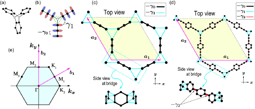
Figure 1: (a) Schematic structure of triptycene molecule. The black and white carbons indicate sp² and sp³ carbons, respectively. Each sp² carbon gives one $\pi$-electron. (b) Top view of the triptycene molecule together with $\pi$-orbital at each sp² carbons. $\pi$-orbitals construct the triangle network drawn with green dashed lines. Schematic structure of (c) zigzag TMM and (d) armchair TMM. The yellow shaded rhombus indicates the unit cell of TMMs. $\bm{a_{1}}=(a,0)$, $\bm{a_{2}}=(-a/2,\sqrt{3}a/2)$ are primitive vectors, where $a=8.92$Å for zigzag TMM and $a=22.17$Å for armchair TMM, respectively. The zigzag and armchair TMMs have $18$ and $54$ $\pi$-electronic sites in their unit cells, respectively. (e) 1st BZ of TMMs.

In this paper, we theoretically study the optical properties of TMMs under the linearly and circularly polarized light irradiation. To analyze the optical properties of TMMs, we construct the tight-binding model that faithfully reproduces the energy band structure obtained by DFT, and numerically evaluate the optical absorption intensity and valley selective optical excitation using the Kubo formula. Kubo (1957); Mahan (2000) It is found that absorption intensity crucially depends on both light polarization angle and the momentum of optically excited electrons. It is also confirmed that the circularly polarized light irradiation can selectively excite the electrons in either $K$ or $K^{\prime}$ point. Then, we analyze the optical selection rule of TMMs using the group theory. From the analysis, we determine the selection rules of the absorption spectrum and polarization-dependent transition at the high symmetric points in 1st BZ.

This paper is organized as follows. In Sec. II, we illustrate the lattice structures of zigzag and armchair TMMs. Subsequently, we construct the tight-binding model to calculate their electronic structures and describe the fundamental theoretical framework to evaluate the optical properties of TMMs. In Sec. III, we discuss the optical properties of zigzag TMM under linearly and circularly polarized light irradiation. The optical properties of armchair TMM is discussed in Sec. IV. Section V summarizes our results. In addition, the details of the optical selection rules for 2D Kagome lattice are given in the Appendix A.

II Tight-binding Model of TMM

In this paper, we employ the tight-binding model to describe the $\pi$-electronic states of TMMs and study their optical properties under the linearly and circularly polarized light irradiation. The Hamiltonian for the $\pi$-orbitals in TMMs can be given as

$$\hat{H}=\sum_{\langle n,m\rangle}\gamma_{n,m}\ket{\psi_{n}}\bra{\psi_{m}},$$

where $\psi_{m}$ and $\psi_{n}$ indicate the $\pi$-orbitals at $m$ and $n$ sites in the unit cell, respectively. $\gamma_{n,m}$ indicates the $\pi$-electron hopping integral between $m$ and $n$ atomic sites. The detailed parametrization of $\gamma_{n,m}$ is given below.

Triptycene is the 3D aromatic molecule and schematically shown in Fig. 1(a). The black and white circles indicate sp² and sp³ carbon atoms, respectively. Each sp² carbon provides one $\pi$-electron. Owing to the central sp³ carbons, three propeller wings extend toward three directions forming C_3v symmetry. Since there is no $\pi$-electron on the center of three propellers, the $\pi$-electrons construct the triangle network in the triptycene. Figure 1(b) shows the top view of triptycene molecule together with $\pi$-orbitals. The electron hoppings within the same wing are defined as $-\gamma_{0}$, and those between different wings are defined as $\gamma_{1}$, where $\gamma_{0}>0$ and $\gamma_{1}>0$.

Figure 2: (a) Energy bands structure of zigzag TMM together with corresponding DOS on the basis of tight-binding model. Black and cyan lines in the energy band structure indicate bonding and anti-bonding states between upper and lower layers, respectively. Note that the optical transition between black and cyan subbands are prohibited. The representative optical transitions from the highest valence subband are named $T_{1}$, $T_{2}$ and $T_{3}$. (b) (Left panel) Corresponding absorption spectrum of $T_{1}$, $T_{2}$ and $T_{3}$ optical transitions. The $k$-integration is performed within the whole 1st BZ. (Right panel) Same for $T_{1}$, $T_{2}$ and $T_{3}$ optical transitions, but the $k$-integration is performed in the $1/3$ regions of 1st BZ which separately contain $M_{1}$, $M_{2}$ and $M_{3}$ points. Angular dependence of absorption intensity at (d) $\Gamma$, (e) $M_{2}$, and (f) $K_{2}$ points.

As shown in Figs. 1 (c) and (d), there are two types of cross-linked structures of TMMs, i.e., zigzag and armchair TMMs, respectively. It should be noted that both of TMMs have C_6v symmetry. Here, the magenta arrows are primitive vectors, given as $\bm{a_{1}}=(a,0)$ and $\bm{a_{2}}=(-\frac{a}{2},\frac{\sqrt{3}a}{2})$, where $a$ is lattice constant: $a=8.92$Å for zigzag TMM and $a=22.17$Å for armchair TMM, respectively. The yellow shaded areas are the unit cells of TMMs. The zigzag and armchair TMMs have $18$ and $54$ $\pi$-electronic sites in their unit cells, respectively. Since the corresponding reciprocal lattice vectors are given as $\bm{b_{1}}=\frac{2\pi}{a}(1,\frac{1}{\sqrt{3}})$ and $\bm{b_{2}}=\frac{2\pi}{a}(0,\frac{2}{\sqrt{3}})$, the 1st BZ for TMMs becomes the hexagonal shown in Fig. 1(e).

In zigzag TMMs, triptycene molecules are polymerized by sharing benzene rings between neighboring molecules. It can be understood that the $\pi$-electrons form the network composed of triangle rings and even membered rings as shown in Fig. 1 (c). The inplane network structure is resemble to the Kagome lattice, where triangle and hexagonal-symmetric rings are alternatively spread. Besides, this Kagome-like network forms the bilayered structure which can be seen in side-view. The bilayer structure leads to bonding and anti-bonding molecular orbitals between upper and lower layers. As shown in Appendix A, the tight-binding model of 2D Kagome lattice produces the energy band structures with graphene energy dispersion and a perfect flat band. In actual, the DFT calculations show that zigzag TMMs become semiconducting and show the energy band structures accompanying several sets of Kagome-like energy dispersion. For the tight-binding model of zigzag TMMs, we use $-\gamma_{0}$ for the electron transfer within benzene rings, $\gamma_{1}=\gamma_{0}/4$ for triangular rings connecting benzene rings. Throughout this paper, we set $\gamma_{0}=2.43$eV. This parameter set fairly reproduces the energy band structures of zigzag TMMs obtained DFT calculations.

Figure 1 (d) shows the lattice structure of armchair TMMs, where triptycene molecules are connected through benzene molecules with $\sigma$-bondings. Since the benzene molecule bridges two carbon atoms belonging to the different layers as shown in the side-view of the structure, armchair TMM has the rippling structure. The DFT study has shown that armchair TMM is energetically stable and semiconducting. Similar to zigzag TMM, owing to the presence of triangle rings, armchair TMMs also has Kagome-like energy band structures. For the tight-binding model of armchair TMM, we use $-\gamma_{0}$ for the electron transfer within benzene rings, $\gamma_{1}=\gamma_{0}/4$ for triangular rings connecting benzene rings. It is also known that the bridging benzene rings are tilted with the angle of $\frac{\pi}{6}$ from the vertical plane to the armchair membrane owing to the conformation. Thus, the transfer integral for the bridging bonds is taken as $-\gamma_{2}(=-\gamma_{0}\cos\theta)$ with $\theta=\frac{\pi}{6}$. This parameter set fairly reproduces the energy band structures of armchair TMMs obtained DFT calculations. Fujii et al. (2018b)

Let us briefly make the overview of theoretical framework to study the optical properties of TMMs under the linearly and circularly polarized light irradiation. The light absorption coefficient of solid is described as

$$\alpha(\omega)=\frac{\omega}{cn}\rm{Im}[\varepsilon{(\omega)}],$$

where $\varepsilon(\omega)$ is complex dielectric function. Here $\omega$ is frequency of irradiation light and $n$ is refractive index. In addition, dielectric function $\varepsilon(\omega)$ can be related to the dynamical conductivity $\sigma(\omega)$ by

$$\varepsilon(\omega)=1+i\frac{4\pi}{\omega}\sigma(\omega).$$

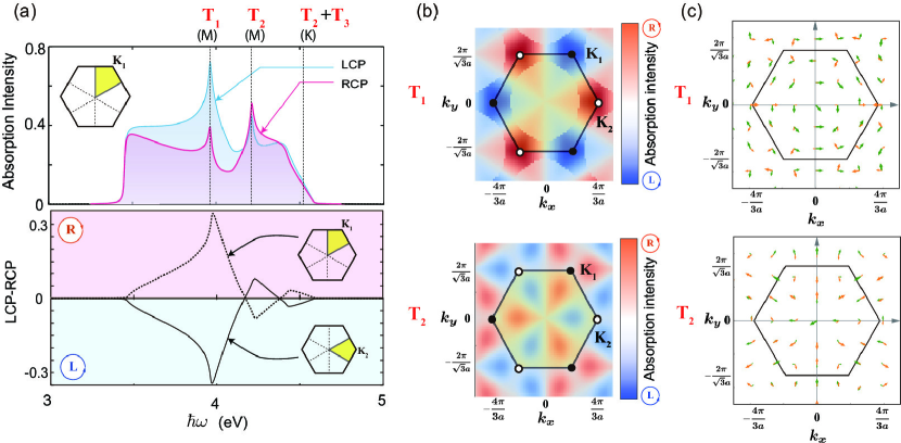
Figure 3: (a) (Upper panel) Optical absorption spectrum of zigzag TMM under the circularly polarized light irradiation. The three dashed lines indicate the representative optical transition caused by $T_{1}$ at $M$ point, $T_{2}$ at $M$ point and $T_{2}+T_{3}$ at $K$ point from left. The integration is evaluated within the $1/6$ region of 1st BZ containing $K_{2}$ point. (Lower panel) The difference of optical absorption between LCP and RCP. Dashed and solid lines correspond to the cases of $k$-integration for the $1/6$ regions of BZ containing $K_{1}$ and $K_{2}$, respectively. Since TMM preserves both time-reversal and inversion symmetries, $K_{1}$ and $K_{2}$ states polarize oppositely, i.e., no net valley polarization. (b) Momentum space mapping of absorption intensity difference between LCP and RCP, i.e., $\Delta\alpha(\bm{k})$ for (upper panel) $T_{1}$ and (lower panel) $T_{2}$ transitions. (c) The distribution of dipole vector in the momentum space for (upper panel) $T_{1}$ and (lower panel) $T_{2}$ transitions under the circularly polarized light irradiation. The green and orange arrows indicate real and imaginary parts of the dipole vector, respectively.

Since the effect of external field is treated within first-order perturbation, the dynamical conductivity can be evaluated through Kubo formula, Kubo (1957); Mahan (2000) i.e.,

$$\sigma(\omega) =\frac{\hbar}{iS}\sum_{\bm{k}}\sum_{i,f}\frac{f{(E_{\bm{k}}^{(f)})}-f{(E_{\bm{k}}^{(i)})}}{E_{\bm{k}}^{(f)}-E_{\bm{k}}^{(i)}}\frac{\left|\bm{e}\cdot\bra{\psi_{\bm{k}}^{(f)}}\nabla_{\bm{r}}\ket{\psi_{\bm{k}}^{(i)}}\right|^{2}}{E_{\bm{k}}^{(f)}-E_{\bm{k}}^{(i)}-\hbar\omega+i\eta}.$$

$$\eqqcolon\frac{1}{S}\sum_{\bm{k}}\sum_{i,f}\tilde{\sigma}_{f,i}(\bm{k},\omega)$$

$S$ is the area of system and $E_{\bm{k}}^{(i)}$ and $E_{\bm{k}}^{(f)}$ indicate the eigenenergies for initial and final states for the inter-band optical transition, respectively. $\psi_{\bm{k}}^{(i)}$ and $\psi_{\bm{k}}^{(f)}$ are corresponding wavefunctions obtained from tight-binding model. The $\bm{k}$-summation is performed within the 1st BZ. $f{(E^{(i)}_{\bm{k}})}$ is the Fermi-Dirac distribution function for the state of energy $E^{(i)}_{\bm{k}}$. $\eta$ is an infinitesimally small real number. Also, $\bm{e}=(e_{x},e_{y})$ is the polarization vector of incident light and $\bra{\psi_{\bm{k}}^{(f)}}\nabla_{\bm{r}}\ket{\psi_{\bm{k}}^{(i)}}$ represents the transition dipole vector, where $\nabla_{\bm{r}}=(\partial/\partial x,\partial/\partial y)$. For later use, we have also defined the integrand of $\sigma(\omega)$ as $\tilde{\sigma}_{f,i}(\bm{k},\omega)$, which gives the momentum resolved aborption intensity from $\psi_{\bm{k}}^{(i)}$ to $\psi_{\bm{k}}^{(f)}$, i.e., $\alpha_{f,i}(\bm{k},\omega)$. This will be used for momentum space mapping of aborption intensity.

The transition dipole vector is evaluated as the expectation value of group velocity, Lew Yan Voon and Ram-Mohan (1993) i.e.,

$$\bra{\psi_{\bm{k}}^{(f)}}\nabla_{\bm{r}}\ket{\psi_{\bm{k}}^{(i)}}=i\frac{m}{\hbar}\bra{\psi_{\bm{k}}^{(f)}}\frac{\partial\hat{H}}{\partial\bm{k}}\ket{\psi_{\bm{k}}^{(i)}}.$$

The inner product between the polarization vector and the transition dipole vector leads to

$$\bm{e}\cdot\bra{\psi_{\bm{k}}^{(f)}}\nabla_{\bm{r}}\ket{\psi_{\bm{k}}^{(i)}}$$

$$=i\frac{m}{\hbar}\left(e_{x}\bra{\psi_{\bm{k}}^{(f)}}\frac{\partial\hat{H}}{\partial\bm{k_{x}}}\ket{\psi_{\bm{k}}^{(i)}}+e_{y}\bra{\psi_{\bm{k}}^{(f)}}\frac{\partial\hat{H}}{\partial\bm{k_{y}}}\ket{\psi_{\bm{k}}^{(i)}}\right).$$

The polarization of light can be incorporated through the Jones vectors. Jones (1941) For linearly polarized light, it is given as

$$\bm{e}_{\rm{Linear}}=\left(\begin{array}[]{c}\cos{\phi}\\ \sin{\phi}\\ \end{array}\right),$$

where $\phi$ is direction of electric field of incident light measured from $x$-axis. Meanwhile, for right-handed circularly polarized (RCP) light irradiation, we use

$$\bm{e}_{\rm{RCP}}=\frac{1}{\sqrt{2}}\left(\begin{array}[]{c}1\\ -i\\ \end{array}\right),$$

and for left-handed circularly polarized (LCP) light, we use

$$\bm{e}_{\rm{LCP}}=\frac{1}{\sqrt{2}}\left(\begin{array}[]{c}1\\ i\\ \end{array}\right).$$

$\bm{e}_{\rm{RCP}}$ and $\bm{e}_{\rm{LCP}}$ satisfy the orthogonality.

III Optical properties of zigzag TMM

In this section, we consider the optical properties of zigzag TMM under linearly and circularly polarized light irradiation. Figure 2 (a) shows the energy band structure of zigzag TMM together with the corresponding density of states (DOS) on the basis of tight-binding model. The system is semiconducting with the direct band gap. Since zigzag TMM has C_6v symmetry same as the 2D Kagome lattice, several Dirac cones appear at $K$-point. Simultaneously, several perfect flat bands appear owing to the nature of Kagome lattice. If we say a set of graphene-like bands with a flat band as a Kagome-like energy band, as we have expected, six set of Kagome-like energy band structures are obtained. Since zigzag TMM has the bilayered structure, we can distinguish the energy subbands into bonding (black line spectrum) and anti-bonding (cyan line spectrum) subbands across the upper and lower layers. It is noted that optical transitions occur between same types of states, i.e., the transition from bonding (anti-bonding) to anti-bonding (bonding) states is forbidden since the parity of the wavefunction is reversed with respect to the $xy$-plane.

III.0.1 Linearly Polarized Light

Let us closely inspect the optical properties of zigzag TMM under linearly polarized light irradiation. To study the details of optical selection rules, we focus on the optical transition from the highest valence subband. The representative optical transitions are named $T_{1}$, $T_{2}$ and $T_{3}$ indicated by red arrows in Fig. 2(a). Note that the optical transition to cyan-colored subband is prohibited. The left panel of Fig. 2(b) shows the incident energy dependence of absorption intensity under linearly polarized light irradiation. Only $T_{1}$, $T_{2}$ and $T_{3}$ transitions contribute optical absorption in this energy region, and $k$-integration is performed in the whole 1st BZ.

The absorption spectrum shows two intensive peaks at $3.96$ and $4.21$ eV, which originate from the divergent joint density of states (JDOS) owing to the saddle points of energy band structure at $M$ points. The first peak mainly arises from the optical transition $T_{1}$, and the second one arises from $T_{2}$.

It is noted that three non-equivalent $M$ points contribute differently to these peaks of the optical absorption spectrum. The right panel of Fig. 2(b) shows the contributions from $M_{1}$, $M_{2}$, and $M_{3}$ points. To separate the contribution from each $M$ point, $\bm{k}$-integration of optical conductivity is performed in the three divided regions as shown in the inset of right panel of Fig. 2(b). It is seen that the $M_{2}$ point has the larger contribution to the first peak than $M_{1}$ and $M_{3}$, but the smaller contribution to the second peak. Thus, it is possible to make a polarization among three non-equivalent $M$ points using the linearly polarized light irradiation.

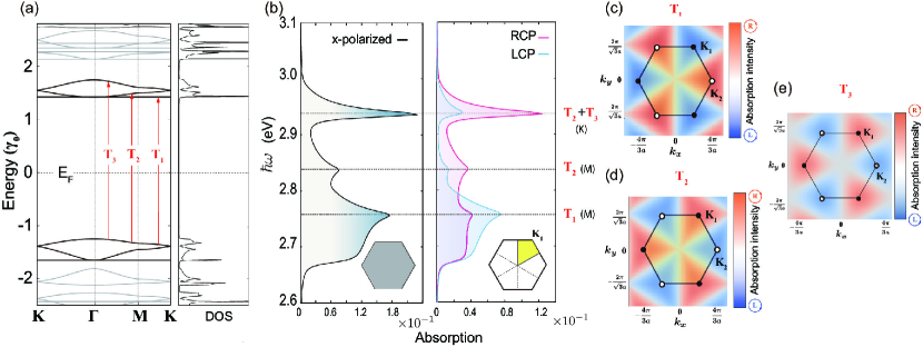
Figure 4: (a) Energy band structure of armchair TMM together with DOS on the basis of tight-binding model. The optical transitions from the highest valence subband to lowest three conduction subbands are named $T_{1}$, $T_{2}$ and $T_{3}$. (b) Optical absorption spectrum of armchair TMM under (left panel) linearly and (right panel) circularly irradiation. For linearly irradiation, $k$-integration is performed for whole 1st BZ. There are three pronounced peaks at $\hbar\omega=2.76$, $2.84$, and $2.94$ eV. At right side of the panel, it is noted that dominant optical transition and the high symmetric points where the optical transitions occur. For circularly irradiation, $k$-integration is performed for the $1/6$ region of 1st BZ containing $K_{1}$. Momentum space mapping of absorption intensity difference between RCP and LCP, i.e., $\Delta\alpha(\bm{k})$ for (c) $T_{1}$, (d) $T_{2}$ and (e) $T_{3}$ transitions.

III.0.2 Polarization Angle Dependence at High Symmetric $k$-Points

Next, we shall discuss the polarization angle dependence of optical absorption intensities at $\Gamma$, $M$, $K$ points using group theory. Dresselhaus et al. (2008) Since the TMMs have similar crystal symmetry with 2D Kagome lattice, the polarization angle dependence is quite analogous to the case of 2D Kagome lattice discussed in Appendix A in detail.

[1] $\Gamma$ point: The $\Gamma$ point has C_6v symmetry. However, in Kagome lattice and TMMs, the optical selection rules are determined by C_3v symmetry, because of the existence of the triangle unit in the lattice. Thus, optical transition occurs between non-degenerate $A_{1}$ state and doubly degenerate $E$ states. Therefore, only $T_{1}$ and $T_{2}$ transitions are optically active, but $T_{3}$ is prohibited.

Figure 2(d) shows the polar angle dependence of light absorption at the $\Gamma$ point for $T_{1}$ and $T_{2}$. Since the wavefunction of zigzag TMM (not shown) has the same symmetry as that of 2D Kagome lattice, the $T_{1}$ and $T_{2}$ have the polarization angle dependence on $\cos\phi$ and $\sin\phi$, respectively.

[2] $M$ point: The $M$ points have C_2v symmetry, i.e., there is no degeneracy in energy dispersion at these points. In zigzag TMM, all the wavefunctions at $M$ points are classified into either $A$ or $B$ representation, as similar to the case of 2D Kagome lattice. The optical transitions occur for $T_{1}$ and $T_{2}$. It should be noted that $T_{3}$ is not allowed because $T_{3}$ connects the two states with the same symmetry. In Fig. 2(e), the angle dependence of linearly polarized light at $M_{2}$ point is shown. We can clearly confirm the $T_{1}$ and $T_{2}$ have $\cos\phi$ and $\sin\phi$ dependence, respectively. This is consistent with the case of 2D Kagome lattice. For $M_{1}$ ($M_{3}$) point, the polarization angle dependence is obtained by shifting the angle as $\phi\rightarrow\phi-\pi/3$ ($\phi+\pi/3$).

[3] ${K}$ point: The $K$ points have C_3v symmetry. Similar to 2D Kagome lattice, non-degenerate $A_{1}$ states and doubly degenerates $E$ states appear at $K$ points in zigzag TMM. The flat band state corresponds to $A_{1}$, and the Dirac points correspond to $E$ states. Thus, the optical transitions are allowed between $A_{1}$ and $E$ states, i.e, $T_{1}$, and between $E$ states, i.e., $T_{2}$ and $T_{3}$. However, it is noted that the optical absorption is relatively weak compared with those at $\Gamma$ and $M$ points, owing to the smaller JDOS of Dirac cones in zigzag TMM.

The angle dependence at $K$ points is shown in Fig. 2(f). It is noted that the optical transition of $T_{1}$ is isotropic, which is not seen in $\Gamma$ and $M$ points. It is equivalent to the polarization dependence of 2D Kagome lattice, see Appendix A.

Furthermore, in TMMs, the unique optical transitions occur between Dirac cones, which are absent in simple 2D Kagome lattice. Similar to graphene, the Dirac cones are expected to have the helicity. In general, the upper and lower cones have opposite helicities even at the same $K$ point. The red and blue Dirac cones in Fig. 2(f) indicate the opposite helicity. It should be noted that the optical transitions between the same (different) helicities have the polarization angle dependence of $\sin\phi$ ($\cos\phi$). Thus, the polarization dependence of absorption spectrum at $K$ points has different origin from those at the $\Gamma$ and $M$ points.

III.0.3 Circularly Polarized Light

Since zigzag TMM has the valley structures in the energy band structure, the circularly polarized light irradiation can selectively excite the electrons belonging to either ${K_{1}}$ or ${K_{2}}$ point depending on the direction of polarization. Note that the present system preserves both time-reversal and inversion symmetries, no net valley polarization occurs. The upper panel of Fig. 3(a) is the absorption spectrum under the circularly polarized light irradiation, where the $k$-integration has been performed within the $1/6$ region of BZ containing $K_{2}$ point, see inset of Fig. 3(a). It can be noticed that there are two pronounced peaks around $\hbar\omega=3.96$ and $4.21$ eV, where only the first peak shows rather large difference between LCP and RCP. The first and second peaks correspond to the optical transition of $T_{1}$ and $T_{2}$ at $M$ point, respectively. The optical transition of $T_{1}$ is mainly dominated by the electronic excitation at $M$ and $K$ points. However, $T_{2}$ is mostly dominated by electronic excitation at $M$ points. The lower panel of Fig. 3(a) is the difference of optical absorption between LCP and RCP. Since TMM preserves both time-reversal and inversion symmetries, $K_{1}$ and $K_{2}$ states polarize oppositely, i.e., no net valley polarization.

Figure 3(b) shows momentum space mappings of absorption intensity differences between LCP and RCP, $\Delta\alpha(\bm{k})$, for the optical transitions $T_{1}$ and $T_{2}$. $\Delta\alpha(\bm{k})$ is defined as $\Delta\alpha(\bm{k})\coloneqq\alpha^{LCP}_{(f,i)}(\bm{k},\omega)-\alpha^{RCP}_{(f,i)}(\bm{k},\omega)$, where $(f,i)$ and $\omega$ are chosen to satisfy the condition of specific optical transition. Red (blue) region indicates strong absorption for RCP (LCP). The strong valley selective excitation by circularly polarized light irradiation can be observed for the optical transition $T_{1}$. However, such valley selective excitation becomes weak for $T_{2}$. This can be understood by inspecting the momentum space mapping of the dipole vector, $\bra{\psi_{\bm{k}}^{(f)}}\nabla_{\bm{r}}\ket{\psi_{\bm{k}}^{(i)}}$ as shown in Fig. 3(c), where green and orange arrows indicate real and imaginary parts of the dipole vector, respectively. As can be seen, the real and imaginary parts are orthogonal near the $K_{1}$ and $K_{2}$ points for $T_{1}$, resulting in the valley selective excitation. Ghalamkari et al. (2018); Tatsumi et al. (2018) However, the real and imaginary parts of dipole vector becomes parallel in the transition $T_{2}$, i.e. very weak valley selective excitation. Note that the momentum mapping of absorption intensity for $T_{3}$ is not shown here, because of that $T_{3}$ is optically prohibited except the vicinity of $K$ points.

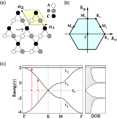
Figure 5: (a) Schematic of 2D Kagome lattice. The yellow area represents the unit cell and the primitive vectors are $\bm{a_{1}}=(a,0)$, $\bm{a_{2}}=(-\frac{a}{2},\frac{\sqrt{3}a}{2})$. $-\gamma$ is the hopping parameter between the nearest-neighbor sites. (b) 1st BZ. (c) Energy band structure and DOS. The optical transition from $\epsilon_{1}$ to $\epsilon_{2}$ ($\epsilon_{3}$) is defined as $T_{1}$ ($T_{2}$).

IV Optical properties of armchair TMM

In this section, we briefly discuss the optical properties of armchair TMM. For armchair TMM, we can apply the similar optical selection rules found in zigzag TMM. However, owing to the less dispersive energy band structures of armchair TMM, rather clear valley selective optical excitation can be observed.

Figure 4(a) shows the energy band structure of armchair TMM together with the corresponding DOS on the basis of tight-binding model. Here the titled angle is set to $\frac{\pi}{6}$. Similarly, several sets of Kagome bands are obtained. Since the unit cell contains $54$ atomic sites, only subbands and DOS near the Fermi energy are shown. Owing to the rippling structure of armchair TMMs, we cannot decompose the energy subbands into bonding and anti-bonding states. Similar to the case of zigzag TMM, let us focus on the optical transition from the highest valence subband to three lowest conduction subbands indicated as $T_{1}$, $T_{2}$, and $T_{3}$ in Fig. 4(a). Note that no valley polarization occurs, because both time-reversal and inversion symmetries are preserved.

In armchair TMM, the absorption spectrum of these transitions has the two strong peaks around the $2.76$eV and $2.94$eV in addition to one weak peak around the $2.84$eV as shown in the left panel of Fig. 4(b). Here, $k$-integration is performed in the whole 1st BZ. The first strong peak and second weak peak indicate the $T_{1}$ and $T_{2}$ transitions at $M$ point, respectively. However, the third strong peak indicates $T_{2}$ and $T_{3}$ transitions at $K$ point. In armchair TMM, the slope of energy dispersion for Dirac cones becomes smaller than that of zigzag TMM, leading to faster increase of DOS near the Dirac points. This fact induces rather strong valley selective optical absorption at $K$ point for $\hbar\omega=2.94$eV. Thus, armchair TMM can generate the valley selective optical excitation more clearly, as shown in the right panel of Fig. 4(b). Here, $k$-integration is performed in the $1/6$ region of 1st BZ containing $K_{1}$ point, see inset of Fig. 4(b). Certainly, the momentum space mappings of the absorption spectrum differences $\Delta\alpha(\bm{k})$ for $T_{1}$, $T_{2}$ and $T_{3}$ transitions clearly indicate the selective excitation around the $K_{1}$ and $K_{2}$ points as shown in Figs. 4(c), (d) and (e).

V Summary

In summary, we have theoretically investigated the optical properties of TMMs under the linearly and circularly polarized light irradiation. To analyze the optical properties of TMMs, we have constructed the tight-binding model that faithfully reproduces the energy band structures obtained by first-principles calculations. On the basis of the tight-binding model, we have numerically evaluated the optical absorption intensity and valley selective optical excitation using the Kubo formula. This approach reduces significantly the computational cost, since the TMMs contain the large number of atoms in their unit cells. It is found that absorption intensity crucially depends on both light polarization angle and the momentum of optically excited electrons. It has been also confirmed that the circularly polarized light irradiation can selectively excite the electrons in either $K$ or $K^{\prime}$ point. Besides the circularly polarized light irradiation, the use of second optical harmonics Golub and Tarasenko (2014) is another way to generate the valley polarization in TMMs, which will be studied in future. Thus, TMMs are considered to be the good platform for the valleytronics applications. In addition, we have analyzed the selection rules of TMMs using group theory, which shows very similar optical selection rules to that of 2D Kagome lattice system. From the analysis, we have determined the absorption spectrum and polarization-dependent transition at high symmetric points in 1st BZ. Our works will serve for designing further TMMs and analyze the experimental data of the optical absorption spectrum of TMMs.

K.W. acknowledges the financial support from Masuya Memorial Research Foundation of Fundamental Research. This work was supported by JSPS KAKENHI Grant No. JP18H01154, and JST CREST Grant No. JPMJCR19T1.

Appendix A Selection Rule of 2D Kagome Lattice

Here we consider the electronic states of 2D Kagome lattice and summarize the optical selection rules on the basis of nearest-neighbor tight-binding model. Figure 5 (a) shows schematic of 2D Kagome lattice. The yellow shaded area is the unit cell, which contains three non-equivalent atomic sites called $A$, $B$ and $C$. The primitive vectors are given as $\bm{a_{1}}=(a,0)$ and $\bm{a_{2}}=(-\frac{a}{2},\frac{\sqrt{3}a}{2})$, where $a$ is the lattice constant. Here, we assume that each site has a single electronic orbital and electron hopping parameter between nearest-neighbor sites is $-\gamma$.

The Schrödinger equation for 2D Kagome lattice is given as

$$\hat{H}_{\bm{k}}\psi_{\bm{k}}=\epsilon_{\bm{k}}\psi_{\bm{k}},$$

where $\psi_{\bm{k}}=\left(A_{\bm{k}},B_{\bm{k}},C_{\bm{k}}\right)$ is the wavefunction representing the amplitude at $A$, $B$ and $C$ subblattice sites in the unit cell, respectively. $\epsilon_{\bm{k}}$ is the energy eigenvalue. The Hamiltonian is given by

$$\hat{H}_{\bm{k}}=-\gamma\left(\begin{array}[]{ccc}0&1+e^{iK_{1}}&1+e^{-iK_{3}}\\ 1+e^{-iK_{1}}&0&1+e^{iK_{2}}\\ 1+e^{iK_{3}}&1+e^{-iK_{2}}&0\end{array}\right).$$

Here, we have defined $K_{\nu}=\bm{k}\cdot\bm{a}_{\nu}/2.$ with $\nu=(1,2,3)$, $\bm{k}=(k_{x},k_{y})$ and $\bm{a_{3}}=-(\bm{a_{1}}+\bm{a_{2}})$. Since the reciprocal lattice vectors are given as $\bm{b_{1}}=\frac{2\pi}{a}(1,\frac{1}{\sqrt{3}})$ and $\bm{b_{2}}=\frac{2\pi}{a}(0,\frac{2}{\sqrt{3}})$, the 1st BZ of 2D Kagome lattice becomes hexagonal shown in Fig. 5(b). The energy eigenvalues are given as $\epsilon_{\bm{k}}/\gamma=2,-1\pm\sqrt{3+2\sum_{\nu=1}^{3}\cos\left({K_{\nu}}\right)}.$ It should be noted that the form $\pm\sqrt{3+2\sum_{\nu=1}^{3}\cos\left({K_{\nu}}\right)}$ is completely identical with the form of energy band dispersion of nearest-neighbor tight binding model for $\pi$-electrons of graphene.

Figure 5(c) shows energy band structure and corresponding density of states of 2D Kagome lattice. There are three subbands in this system, the two lowest subbands have the identical structure with that of 2D honeycomb lattice, i.e., graphene. However, there is the perfect flat band over the 1st BZ at $\epsilon=2\gamma$. Hereafter, we call the energy subband $\epsilon_{1}$, $\epsilon_{2}$ and $\epsilon_{3}$ from lowest one to highest one, and corresponding wavefunctions $\psi_{1}$, $\psi_{2}$ and $\psi_{3}$, respectively. We also define that the optical transition from $\epsilon_{1}$ to $\epsilon_{2}$ ($\epsilon_{3}$) as $T_{1}$ ($T_{2}$).

Table 1: Character table of $C_{6v}$

$C_{6v}$	$E$	$2C_{6}(z)$	$2C_{3}(z)$	$C_{2}(z)$	$3\sigma_{v}$	$3\sigma_{d}$
$A_{1}$	1	1	1	1	1	1	$z$
$A_{2}$	1	1	1	1	-1	-1
$B_{1}$	1	-1	1	-1	1	-1
$B_{2}$	1	-1	1	-1	-1	1
$E_{1}$	2	1	-1	-2	0	0	$(x,y)$
$E_{2}$	2	-1	-1	2	0	0

Table 2: Character table of $C_{3v}$

$C_{3v}$	$E$	$2C_{3}(z)$	$3\sigma_{v}$
$A_{1}$	1	1	1	$z$
$A_{2}$	1	1	-1
$E$	2	-1	0	$(x,y)$

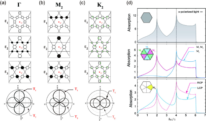
Figure 6: The real space distribution of wave functions for 2D Kagome lattice and (bottom panel) corresponding angle dependence of optical absorption at high symmetric points: (a) $\Gamma$ and (b) $M_{2}$. Black and white circles indicate the sign of wave functions, and the radius of circles indicates the amplitude of wave functions. Red dots indicate the inversion center (IC) of Kagome lattice. (c) Same for $K_{2}$ point. Here, the argument of complex wave function is indicated by green arrows. (d) Absorption intensity and polarization of 2D Kagome lattice, where $k$-integration for optical conductivity is performed (upper panel) for the whole 1st BZ, (middle panel) for $1/3$ regions of 1st BZ containing either $M_{1}$, $M_{2}$ or $M_{3}$ point, (lower panel) for $1/6$ region of 1st BZ containing $K_{2}$ point.

Let us discuss the optical selection rules and polarization angle dependence of 2D Kagome lattice at high symmetric $\bm{k}$-points, i.e., $\Gamma=(0,0)$, $K_{2}=\frac{2\pi}{a}(\frac{2}{3},0)$, and $M_{1}=\frac{2\pi}{a}(0,\frac{1}{\sqrt{3}})$.

[1] $\Gamma$ point: The $\Gamma$ point has C_6v symmetry, which obeys the character table of Table 1. At $\Gamma$ point, the eigenenergies are $\epsilon_{1}=-4\gamma$, and $\epsilon_{2}=\epsilon_{3}=2\gamma$. The wavefunction is analytically given as

$$\psi^{\Gamma}_{1} =\frac{1}{\sqrt{3}}\left(1,1,1\right),$$

$$\psi^{\Gamma}_{2} =\sqrt{\frac{2}{3}}\left(-\frac{1}{2},-\frac{1}{2},1\right),$$

$$\psi^{\Gamma}_{3} =\frac{1}{\sqrt{2}}\left(1,-1,0\right),$$

which are schematically drawn in Fig 6(a). According to the character table of C_6v, $\psi_{1}$ is $A_{1}$ representation, and the degenerate states of $\psi_{2}$ and $\psi_{3}$ are $E_{2}$ representation. Since the polarization vectors belong to $E_{1}$ representation, the tensor product $E_{1}\otimes A_{1}=E_{1}$ indicates that the optical transition to $E_{2}$ is not allowed. However, it should be noted that 2D Kagome lattice contains C_3v symmetry if we take the triangle unit as the symmetry center. According to the character table of C_3v (see Table 2), $\psi_{1}$ is $A_{1}$ representation, and the degenerate states of $\psi_{2}$ and $\psi_{3}$ are $E$ representation. Since in C_3v the tensor product is given as $E\otimes A_{1}=E$, both of optical transitions $T_{1}$ and $T_{2}$ are active. Furthermore, the basis functions for $\psi_{1}$, $\psi_{2}$ and $\psi_{3}$ states are given as $z$, $y$, $x$, respectively. The optical transition $T_{1}$ and $T_{2}$ have $x$ and $y$ polarization, respectively.

Since the wavefunctions are analytically obtained, we can analytically evaluate expectation values of the optical dipole vectors. For linear polarization, we obtain

$$\bm{e}\cdot\langle\psi_{2}|\nabla_{\bm{k}}H|\psi_{1}\rangle =-i\frac{3\sqrt{3}a}{2\sqrt{2}}\sin\phi,$$

$$\bm{e}\cdot\langle\psi_{3}|\nabla_{\bm{k}}H|\psi_{1}\rangle =i\frac{3a}{\sqrt{6}}\cos\phi.$$

This polarization angle dependence is consistent with the numerical calculations as shown in the bottom panel of Fig. 6(a). For circularly polarization, we obtain

$$\left|\bm{e}_{LCP}\cdot\langle\psi_{j}|\nabla_{\bm{k}}H|\psi_{1}\rangle\right|^{2} =\left|\bm{e}_{RCP}\cdot\langle\psi_{j}|\nabla_{\bm{k}}H|\psi_{1}\rangle\right|^{2},$$

where $j=2,3$. Thus, there is no dependence on direction of circularly polarization at $\Gamma$ point.

Table 3: Character table of $C_{2v}$

$C_{2v}$	$E$	$C_{2}$	$\sigma_{v}(xz)$	$\sigma_{v^{\prime}}(yz)$
$A_{1}$	1	1	1	1	$z$
$A_{2}$	1	1	-1	-1
$B_{1}$	1	-1	1	-1	$x$
$B_{2}$	1	-1	-1	1	$y$

[2] $M$ point: The $M$ points have C_2v symmetry, which obeys the character table of Table 3. The eigenenegies are $\epsilon_{1}=-2\gamma$, $\epsilon_{2}=0$, and $\epsilon_{3}=2\gamma$, respectively. For example, the wavefunctions at $M_{2}$ point are given as

$$\psi^{M_{2}}_{1} =\frac{1}{\sqrt{2}}\left(1,1,0\right),$$

$$\psi^{M_{2}}_{2} =\left(0,0,1\right),$$

$$\psi^{M_{2}}_{3} =\frac{1}{\sqrt{2}}\left(1,-1,0\right),$$

which are schematically shown in Fig. 6 (b). Since C_2v is 1D representation, we can define two symmetry axes in real space. $\psi^{M_{2}}_{1}$, $\psi^{M_{2}}_{2}$, and $\psi^{M_{1}}_{3}$ along the $x$ ($y$) direction are $A_{1}$, $A_{1}$ and $B_{1}$ ($B_{2}$, $A_{1}$ and $A_{1}$) representations, respectively. Note that the basis functions for $B_{1}$ and $B_{2}$ are $x$ and $y$, respectively. Thus, optical transition $T_{1}$ ($T_{2}$) is active with $y$ ($x$) polarization. For linear polarization, we can explicitly write the expectation value of dipole vector as

$$\bm{e}\cdot\langle\psi^{M_{2}}_{2}|\nabla_{\bm{k}}H|\psi^{M_{2}}_{1}\rangle =-i\sqrt{\frac{3}{2}}\sin\phi,$$

$$\bm{e}\cdot\langle\psi^{M_{2}}_{3}|\nabla_{\bm{k}}H|\psi^{M_{2}}_{1}\rangle =-i\cos\phi.$$

$M_{2}$ point has mirror with respect to $k_{y}$ axis, however, $M_{1}$ and $M_{3}$ have the mirror with respect to $k_{y}=\frac{1}{\sqrt{3}}k_{x}$ and $k_{y}=-\frac{1}{\sqrt{3}}k_{x}$, respectively. Thus, polarization angle dependence for $M_{1}$ and $M_{3}$ can be obtained by replacing the result of $M_{2}$ as $\phi\rightarrow\phi-\pi/3$ and $\phi\rightarrow\phi+\pi/3$, respectively. Thus, by tuning the angle of linear polarization, the electrons can be optically excited either $M_{1}$, $M_{2}$ or $M_{3}$ point selectively.

[3] $K_{2}$ point: The $K_{1}$ and $K_{2}$ points have C_3v symmetry. The eigenenergies are $\epsilon_{1}=\epsilon_{2}=-\gamma$ and $\epsilon_{3}=2\gamma$. The wavefunction at $K_{2}$ point is given as

$$\psi^{K_{2}}_{1} =\frac{1}{\sqrt{2}}(-\omega^{-1},0,1),$$

$$\psi^{K_{2}}_{2} =\frac{1}{\sqrt{2}}(1-2\omega,2,-\omega^{-1}),$$

$$\psi^{K_{2}}_{3} =\frac{1}{\sqrt{3}}(\omega^{-1},\omega,1),$$

where $\omega=\exp\left(i\frac{2\pi}{3}\right)$. $\psi_{3}$ has $A_{1}$ representation, and degenerate states of $\psi_{1}$ and $\psi_{2}$ have $E$ representation. For degenerate $\psi_{1}$ and $\psi_{2}$ states, we made the orthonormalization. Since the tensor product leads to $E\otimes E=A_{1}$, the optical transition from Dirac cone to the flat band is active.

For linear polarization, we can explicitly write the expectation value of dipole vector as

$$\bm{e}\cdot\langle\psi^{K_{2}}_{3}|\nabla_{\bm{k}}H|\psi^{K_{2}}_{1}\rangle =-i\frac{\sqrt{3}}{2\sqrt{2}}\omega^{-1}\exp\left(i\phi\right),$$

$$\bm{e}\cdot\langle\psi^{K_{2}}_{3}|\nabla_{\bm{k}}H|\psi^{K_{2}}_{2}\rangle =\frac{\sqrt{3}}{2\sqrt{2}}\omega^{-1}\exp\left(-i\phi\right).$$

The polarization angle works only for the phase factor, i.e., no polarization angle dependence. This behavior is shown in the bottom panel of Fig. 6(c). For circularly polarized light, the expectation values of dipole vector are written as

$$\bm{e}_{RCP}\cdot\langle\psi^{K_{2}}_{3}|\nabla_{\bm{k}}H|\psi^{K_{2}}_{1}\rangle =-i\frac{\sqrt{3}}{\sqrt{2}}\omega^{-1},$$

$$\bm{e}_{LCP}\cdot\langle\psi^{K_{2}}_{3}|\nabla_{\bm{k}}H|\psi^{K_{2}}_{1}\rangle =0,$$

$$\bm{e}_{RCP}\cdot\langle\psi^{K_{2}}_{3}|\nabla_{\bm{k}}H|\psi^{K_{2}}_{2}\rangle =\frac{\sqrt{3}}{\sqrt{2}}\omega^{-1},$$

$$\bm{e}_{LCP}\cdot\langle\psi^{K_{2}}_{3}|\nabla_{\bm{k}}H|\psi^{K_{2}}_{2}\rangle =0.$$

Thus, only RCP light can excite electrons at $K_{1}$ points, i.e., valley selective optical excitation. On the contrary, at $K_{2}$ points, only LCP light can excite electrons. However, it is noted that the optical absorption is relatively weak compared with those at $\Gamma$ and $M$ points, owing to the smaller JDOS of Dirac cones.

Absorption intensity: Figure 6 (d) shows the energy dependence of absorption intensity for the linearly and circularly polarized light irradiation, together with the valley selective optical excitation. In upper pannel of Fig. 6 (d), the spectrum is integrated over the whole 1st BZ, and the sharp peaks at $\hbar\omega=2\gamma$ and $4\gamma$ are originated from optical transition at $M$ point, where JDOS diverges logarithmically.

It is intriguing that the lower peak at $2\gamma$ is dominated by the optical transition $T_{1}$, as shown in middle panel of Fig. 6 (d). This behavior is attributed to the angle dependence at $M$ point showed in Fig. 6 (b). Thus, the lower peak has strong momentum selectivity for the optical absorption. For higher peak at $4\gamma$, no such strong selectivity is found. Also, for circularly polarized light irradiation, such strong polarization dependence does not occur as shown in lower panel of Fig. 6 (d). Instead, the valley selective optical excitation is relatively enhanced around $\hbar\omega=3\gamma$. Around this energy, optical transition occurs mainly at $K$ points between Dirac cones and flat band. Although the optical absorption intensity is not so large owing to the relatively small DOS near Dirac cones, they show stronger valley selective optical exciation.

References

- Chhowalla et al. (2013) M. Chhowalla, H. Shin, G. Eda, L. Li, K. Loh, and H. Zhang, Nat. Chem. 5, 263 (2013).
- Butler et al. (2013) S. Z. Butler, S. M. Hollen, L. Cao, Y. Cui, J. A. Gupta, H. R. Guti’errez, T. F. Heinz, S. S. Hong, J. Huang, A. F. Ismach, E. Johnston-Halperin, M. Kuno, V. V. Plashnitsa, R. D. Robinson, R. S. Ruoff, S. Salahuddin, J. Shan, L. Shi, M. G. Spencer, M. Terrones, W. Windl, and J. E. Goldberger, ACS Nano 7, 2898 (2013).
- Novoselov et al. (2005a) K. S. Novoselov, A. K. Geim, S. V. Morozov, D. Jiang, M. I. Katsnelson, I. V. Grigorieva, S. V. Dubonos, and A. A. Firsov, Nature 438, 197–200 (2005a).
- Dean et al. (2010) C. R. Dean, A. F. Young, I. Meric, C. Lee, L. Wang, S. Sorgenfrei, K. Watanabe, T. Taniguchi, P. Kim, K. L. Shepard, and J. Hone, Nat. Nanotechnol. 5, 722 (2010).
- Novoselov et al. (2005b) K. S. Novoselov, A. K. Geim, S. V. Morozov, D. Jiang, M. I. Katsnelson, I. V. Grigorieva, S. V. Dubonos, and A. A. Firsov, Nature 438, 197 (2005b).
- Zhang et al. (2005) Y. Zhang, Y.-W. Tan, H. L. Stormer, and P. Kim, Nature 438, 201 (2005).
- Cao et al. (2018) Y. Cao, V. Fatemi, S. Fang, K. Watanabe, T. Taniguchi, E. Kaxiras, and P. Jarillo-Herrero, Nature 556, 43 (2018).
- Castro Neto et al. (2009) A. H. Castro Neto, F. Guinea, N. M. R. Peres, K. S. Novoselov, and A. K. Geim, Rev. Mod. Phys. 81, 109 (2009).
- Schaibley et al. (2016) J. R. Schaibley, H. Yu, G. Clark, P. Rivera, J. S. Ross, K. L. Seyler, W. Yao, and X. Xu, Nat. Rev. Mater. 1, 16055 (2016).
- Rycerz et al. (2007) A. Rycerz, J. Tworzydło, and C. W. J. Beenakker, Nat. Phys. 3, 172 (2007).
- Xiao et al. (2007) D. Xiao, W. Yao, and Q. Niu, Phys. Rev. Lett. 99, 236809 (2007).
- Gunlycke and White (2011) D. Gunlycke and C. T. White, Phys. Rev. Lett. 106, 136806 (2011).
- Golub et al. (2011) L. E. Golub, S. A. Tarasenko, M. V. Entin, and L. I. Magarill, Phys. Rev. B 84, 195408 (2011).
- Mak et al. (2014) K. F. Mak, K. L. McGill, J. Park, and P. L. McEuen, Science 344, 1489 (2014).
- Wang et al. (2012) Q. H. Wang, K. Kalantar-Zadeh, A. Kis, J. N. Coleman, and M. S. Strano, Nat. Nanotechnol. 7, 699 (2012).
- Xiao et al. (2012) D. Xiao, G.-B. Liu, W. Feng, X. Xu, and W. Yao, Phys. Rev. Lett. 108, 196802 (2012).
- Zeng et al. (2012) H. Zeng, J. Dai, W. Yao, D. Xiao, and X. Cui, Nat. Nanotechnol. 7, 490 (2012).
- Kioseoglou et al. (2012) G. Kioseoglou, A. Hanbicki, M. Currie, A. Friedman, D. Gunlycke, and B. Jonker, Appl. Phys. Lett. 101 (2012).
- Sallen et al. (2012) G. Sallen, L. Bouet, X. Marie, G. Wang, C. R. Zhu, W. P. Han, Y. Lu, P. H. Tan, T. Amand, B. L. Liu, and B. Urbaszek, Phys. Rev. B 86, 081301(R) (2012).
- Wu et al. (2013) S. Wu, C. Huang, G. Aivazian, J. S. Ross, D. H. Cobden, and X. Xu, ACS Nano 7, 2768 (2013).
- Mielke (1999) A. Mielke, J. Phys. A: Math. Gen. 25, 4335 (1999).
- Helton et al. (2007) J. S. Helton, K. Matan, M. P. Shores, E. A. Nytko, B. M. Bartlett, Y. Yoshida, Y. Takano, A. Suslov, Y. Qiu, J.-H. Chung, D. G. Nocera, and Y. S. Lee, Phys. Rev. Lett. 98, 107204 (2007).
- Yan et al. (2011) S. Yan, D. Huse, and S. White, Science (New York, N.Y.) 332, 1173 (2011).
- Sachdev (1992) S. Sachdev, Phys. Rev. B 45, 12377 (1992).
- Liu et al. (2010) G. Liu, S.-L. Zhu, S. Jiang, F. Sun, and W. M. Liu, Phys. Rev. A 82, 053605 (2010).
- Liu et al. (2009) G. Liu, P. Zhang, Z. Wang, and S.-S. Li, Phys. Rev. B 79, 035323 (2009).
- Guo and Franz (2009) H.-M. Guo and M. Franz, Phys. Rev. B 80, 113102 (2009).
- Hatsugai and Maruyama (2011) Y. Hatsugai and I. Maruyama, EPL 95, 20003 (2011).
- Beugeling et al. (2012) W. Beugeling, J. C. Everts, and C. Morais Smith, Phys. Rev. B 86, 195129 (2012).
- Ezawa (2018) M. Ezawa, Phys. Rev. Lett. 120, 026801 (2018).
- Bolens and Nagaosa (2019) A. Bolens and N. Nagaosa, Phys. Rev. B 99, 165141 (2019).
- Makiura et al. (2010) R. Makiura, S. Motoyama, Y. Umemura, H. Yamanaka, O. Sakata, and H. Kitagawa, Nat. Mater. 9, 565 (2010).
- Colson et al. (2011) J. W. Colson, A. R. Woll, A. Mukherjee, M. P. Levendorf, E. L. Spitler, V. B. Shields, M. G. Spencer, J. Park, and W. R. Dichtel, Science 332, 228 (2011).
- Spitler et al. (2011) E. L. Spitler, B. T. Koo, J. L. Novotney, J. W. Colson, F. J. Uribe-Romo, G. D. Gutierrez, P. Clancy, and W. R. Dichtel, J. Am. Chem. Soc. 133, 19416 (2011).
- Kambe et al. (2013) T. Kambe, R. Sakamoto, K. Hoshiko, K. Takada, M. Miyachi, J.-H. Ryu, S. Sasaki, J. Kim, K. Nakazato, M. Takata, and H. Nishihara, J. Am. Chem. Soc. 135, 2462 (2013).
- Wang et al. (2013) Z. F. Wang, N. Su, and F. Liu, Nano Lett. 13, 2842 (2013).
- Bartlett et al. (1942) P. D. Bartlett, M. J. Ryan, and S. G. Cohen, J. Am. Chem. Soc. 64, 2649 (1942).
- Zhang et al. (2012) C. Zhang, Y. Liu, B. Li, B. Tan, C.-F. Chen, H.-B. Xu, and X.-L. Yang, ACS Macro Lett. 1, 190 (2012).
- Bhola et al. (2013) R. Bhola, P. Payamyar, D. J. Murray, B. Kumar, A. J. Teator, M. U. Schmidt, S. M. Hammer, A. Saha, J. Sakamoto, A. D. Schlüter, and B. T. King, J. Am. Chem. Soc. 135, 14134 (2013).
- Fujii et al. (2018a) Y. Fujii, M. Maruyama, K. Wakabayashi, K. Nakada, and S. Okada, J. Phys. Soc. Jpn. 87, 034704 (2018a).
- Fujii et al. (2018b) Y. Fujii, M. Maruyama, and S. Okada, Jpn. J. Appl. Phys. 57, 125203 (2018b).
- Kubo (1957) R. Kubo, J. Phys. Soc. Jpn. 12, 570 (1957).
- Mahan (2000) G. D. Mahan, Many-Particle Physics (Springer, 2000).
- Lew Yan Voon and Ram-Mohan (1993) L. C. Lew Yan Voon and L. R. Ram-Mohan, Phys. Rev. B 47, 15500 (1993).
- Jones (1941) R. C. Jones, J. Opt. Soc. Am. 31, 488 (1941).
- Dresselhaus et al. (2008) M. S. Dresselhaus, G. Dresselhaus, and A. Jorio, Group Theory (Springer-Verlag Berlin Heidelberg, 2008).
- Ghalamkari et al. (2018) K. Ghalamkari, Y. Tatsumi, and R. Saito, J. Phys. Soc. Jpn. 87, 024710 (2018).
- Tatsumi et al. (2018) Y. Tatsumi, T. Kaneko, and R. Saito, Phys. Rev. B 97, 195444 (2018).
- Golub and Tarasenko (2014) L. E. Golub and S. A. Tarasenko, Phys. Rev. B 90, 201402(R) (2014).