Self-awareness based resource allocation strategy for containment of epidemic spreading

Abstract

Resource support between individuals is of particular importance in controlling or mitigating epidemic spreading, especially during pandemics. Whereas there remains the question of how we can protect ourselves from being infected while helping others by donating resources in fighting against the epidemic. To answer the question, we propose a novel resource allocation model by considering the awareness of self-protection of individuals. In the model, a tuning parameter is introduced to quantify the reaction strength of individuals when they are aware of the disease. And then, a coupled model of resource allocation and disease spreading is proposed to study the impact of self-awareness on resource allocation and, its impact on the dynamics of epidemic spreading. Through theoretical analysis and extensive Monte Carlo simulations, we find that in the stationary state, the system converges to two states: the whole healthy or the completely infected, which indicates an abrupt increase in the prevalence when there is a shortage of resources. More importantly, we find that too cautious and too selfless for the people during the outbreak of an epidemic are both not suitable for disease control. Through extensive simulations, we find the optimal point, at which there is a maximum value of the epidemic threshold, and an outbreak can be delayed to the greatest extent. At last, we study further the effects of network structure on the coupled dynamics. We find that the degree heterogeneity promotes the outbreak of disease, and the network structure does not alter the optimal phenomenon in behavior response.

I Introduction

Controlling the outbreak of epidemic spreading is one of the most important topics in human history. During the past decades, the onset of several major global health threats such as the 2003 spread of SARS, the H1N1 influenza pandemic in 2009, and the western Africa Ebola outbreaks in 2014 have deprived tens of thousands of lives all around the world Chan et al. (2003); Girard et al. (2010); Team (2014). In the present, a novel coronavirus (2019-nCoV) causing severe acute respiratory disease emerged in Wuhan, China. As of February 4, 2020, there have been 20528 confirmed 2019-nCoV infections reported in 33 provinces and municipalities emergency office National Health Commission of the People’s Republic of China . The surge in infections has led to a severe shortage of medical resources. Thousands of confirmed and suspected cases await treatment. Facing the rapid outbreak of disease, people all over the country contribute a resource to support the populations in the epidemic areas, whereas self-protection is also essential. Thus the immediate problem is how can we protect ourselves from being infected while helping others in fighting against the epidemic.

A large number of researchers from various disciplines have made efforts to study the topic of optimal resource allocation in disease suppressing in the past years Wan et al. (2008); Gourdin et al. (2011); Lokhov and Saad (2017); Zhao et al. (2018); Li et al. (2020). For example, Preciado et al.  Preciado et al. (2013) studied the problem of the optimal distribution of vaccination resources to control epidemic spreading based on complex networks. They fond the cost-optimal distribution of vaccination resource when different levels of vaccination are allowed through a convex framework. Further they studied problems of the optimal allocation of two typical resources in containing epidemic spreading, namely the preventive resources and corrective resources throughout the nodes of the network to achieve the highest level of containment when the budget is given in advance or finding the minimum budget required to control the spreading the process when the budget is not specified Preciado et al. (2014). By using geometric programming, they solved these two problems. Chen et al. Chen et al. (2017) solved the problem of optimal allocation of a limited medical resource based on mean-field theory. They found that if the resource quantity that each node could get is proportional to its degree, the disease can be suppressed to the greatest extent. The above works considered the problem from a perspective of mathematical. The problem is solved from the premise that both the number of resources and the spreading state of the epidemic are fixed.

However, the real scenario is more complicated than a static mathematical problem. Multiple dynamical processes always interact and co-evolve Granell et al. (2013); Pastor-Satorras et al. (2015), forming a more realistic starting point. For example, although, the outbreak of 2019-nCoV induce a severe shortage of food, medical and defense resources such as surgical mask and disinfectant within a short time, with more and more resources produced by the healthy people, and the social-support from home and abroad, the situation is beginning to ease in Wuhan. More resources could help curb the spread of the disease. Resources and disease always interact dynamically in the evolution process. The coevolution of multiple dynamical processes attracts extensive research in recent years Wang et al. (2019). Böttcher Böttcher et al. (2015) studied the coevolution of resource and epidemics, they found a critical recovery cost that if the cost is above the critical value, epidemics spiral out of control into “explosive” spread. Chen et al. Chen et al. (2018a) studied the effect of social support from local connections on the spreading dynamics of the epidemic. They proposed coevolution spreading model on multiplex networks and found a hybrid phase transition on networks with heterogeneous degree distribution. In this multiplex network framework, Chen et al.  Chen et al. (2018b) further impact of preferential resource allocation on social subnetwork on the spreading dynamics of the epidemic. They found that the model exhibits different types of phase transitions, depending on the preference value of resource allocation.

In addition to the physical resource that can directly mitigate or control the epidemic spreading, the awareness of the epidemic in populations is another type of resource. The public can perceive the threat of epidemic social network through platform and mass media and then take measure to self-protect. Thus the interplay between awareness and epidemic spreading is another topic that attracts extensive research. A mass of works addressed the problem from different perspectives considering, for example, the risk perception, behavioral changes Funk et al. (2010a); Wu et al. (2012); Yang et al. (2019). Granell et al.  Granell et al. (2013) studied the interplay between the spreading of an the epidemic, and the information awareness on top of multiplex networks. Leveraging a microscopic Markov chain approach they found that the threshold of the epidemics has a metacritical the point from which the onset increases and the epidemics incidence decreases. Wang et al. Wang et al. (2016) studied the coevolution mechanisms using both real online and offline data, and proposed a coupled model on multiplex network. They found that disease outbreak in contact the network can trigger the outbreak of information on a communication network, and found an optimal information transmission rate that markedly suppresses the disease spreading.

Awareness of epidemic spreading is critically essential in suppressing disease outbreak, although there is a mass of works about the coevolution of awareness diffusion and disease spreading, a question remains to study. Namely, how awareness influences individual behavior during the outbreak of disease. The more interesting question is, how individuals will decide whether to allocate their resources after perceiving the local transmission state. To answer these questions, a novel resource allocation model is proposed in this paper, which considers the influence of the awareness of each individual. We consider that healthy individuals in an outbreak of disease are the source of various resources, they can not only produce a medical resource such as drugs, surgical mask but also donate a resource such as funds and food. Whereas when they perceive the threat of disease in the local area, they would decide whether to donate resources to infected neighbors. Since the donation behavior will lead to less resource for self-protection, and a more significant probability to be infected. Whereas, when they are aware of the threat of the disease and refuse to donate resources, they will have more resources for self-protection and a lower probability of being infected. Moreover, to study the interplay between the resource allocation and disease spreading, we propose a coupled dynamical model on complex networks.

Further, we adopt the dynamic message-passing method to solve the coupled model theoretically. First of all, we investigate the influence of awareness on the coupled dynamics of resource allocation and disease spreading on the scale-free network. To quantify the reaction strength of healthy individuals to the information of the local infection state, a parameter $\alpha$ is defined. A larger value of $\alpha$ indicates more sensitivity of an individual to the disease, and lower intention to denote resources. Through theoretical analysis and numeric simulations, we find that the system has only two stationary states, namely the absorb state and the globe outbreak state. With the increase of $\alpha$, the epidemic threshold first increases and then decreases, which indicates an optimal value of $\alpha$. Further, we find the optimal value at $\alpha_{opt}$ through extensive simulations, at which the disease can be suppressed to the greatest extent. Then we explain qualitatively the optimal phenomenon. At last, we investigate the impact of degree heterogeneity on the coupled dynamics, and find that the degree heterogeneity does not alter the optimal phenomenon and the abrupt increase in prevalence with a shortage of resource, and the epidemic threshold increases with the decrease of degree heterogeneity, which suggests that network heterogeneity promotes the outbreak of disease.

II Model descritption

II.1 Epidemic model

A resource based epidemiological susceptible-infected-susceptible model (r-SIS) is proposed to describe coupled dynamics of epidemic spreading and resource allocation on complex network. Individuals are represented by nodes in the network and an adjacency matrix $\mathbb{A}$ is introduced to represent the connection between nodes. If there is an edge between nodes $i$ and $j$, the element $a_{ij}=1$, otherwise $a_{ij}=0$. According to this scheme, any individual can be in two different states: susceptible(S) and infected(I). The infection propagates between each pair of I-state and S-state neighbors with an infection rate $\widetilde{\lambda}$ in one contact, which is assumed to depend on whether the S-state nodes to donate resources, see the details in Sec. II.2. At any time $t$, each I-state node $i$ recovers with a recovery rate $r_{i}(t)$. Resource including the medical, funds and food can promote recovery of patients from disease  Kulik and Mahler (1989); Nausheen et al. (2009). Thus we define the recovery rate of each I-state node as a function of the resource quantity received from healthy neighbors in this paper. As each I-state node will get a different amount of resource, the recovery rate varies from node to node. Consequently, the the recovery rate of any node $i$ at time $t$ can be defined as

$$r_{i}(t)=1-(1-\mu)^{\varepsilon{\omega_{i}(t)}},$$ (1)

where $\omega_{i}(t)$ is resource quantity of node $i$ received from healthy neighbors at time $t$, and $\mu$ is the basic recovery rate. A parameter $\varepsilon\in[0,1]$ is introduced in our model to represent the resource utilization rate  Mackie et al. (2007). Since in real scenario, there is the common phenomenon of the waste on resource Jaarsma et al. (1999); Gul and Guneri (2012) in medical and other service systems, implying the resource received from healthy neighbors may not be fully utilized on curing and recovery. Without loss of generality, we set $\mu_{r}=0.6$ throughout this work, i.e., only $60\%$ of the resources received are used.

For the r-SIS model, we define $\rho_{i}(t)$ is the probability that any node $i$ is an infected state. The fraction of infected nodes in a network of size $N$ at time $t$ can be calculated by averaging overall $N$ nodes:

$$\rho(t)=\frac{1}{N}\sum_{i=1}^{N}\rho_{i}(t).$$ (2)

Further we define the prevalence of the disease in the stationary state as $\rho\equiv\rho(\infty)$

II.2 Resource allocation model based on behaviour response

In the real scenario, healthy individuals can produce resources. For simplicity, we consider that each individual (node) in the network can generate one unit resource at a time step. During an outbreak of a disease, the susceptible individuals can perceive the threat of the disease intuitively by acquiring the information from direct neighbors. Generally, the more infected neighbors of an individual, the deeper it will be aware of the disease Funk et al. (2010b); Wang et al. (2015a). People aware of the disease will have different reactions  Funk et al. (2010b). And to quantify the reaction strength of an individual to the local information of disease, a tuning parameter $\alpha$ is introduced. Based on the description above, we can define the probability that a healthy individual with $m$ infected neighbors donate resource as

$$q(m)=q_{0}(1-\alpha)^{m},$$ (3)

where $q_{0}$ is a basic donation probability. When $\alpha=0$, all healthy nodes have the same donation probability $q_{0}$. Besides, we consider that a healthy node will donate one unit resource equally to its I-state neighbors at a time. Based on the resource allocation scheme, the amount of resource $\omega_{j\rightarrow{i}}$ that node $j$ with $m$ infected neighbors donate to one of its I-state neighbor, $i$ can be expressed as

$$\omega_{j\rightarrow i}=q(m)\frac{1}{m}.$$ (4)

When disease breaks out in the human population, people aware of a disease in their proximity will take measures to reduce their susceptibility, leading to a reduction in the effective rate of infection  Funk et al. (2009); Granell et al. (2013). We consider that if an individual is aware and refuse to donate resource for self-protection, it reduces its infectivity by a factor $c$. The basic infection rate is denoted as $\lambda$, and the actual rate of infection is denoted as $\widetilde{\lambda}$, which can thus be expressed as

$$\widetilde{\lambda}=\left\{\begin{array}[]{ll}\lambda,&\hbox{if distribute the resources;}\\ c\lambda,&\hbox{else. }\end{array}\right.$$ (5)

If a healthy individual donate resource to infected neighbors, it has a larger probability to be infected, on the contrary, it has a relatively smaller probability to be infected. The effective infection rate of any node $i$ can be also expressed as a function of $q$,

$$\widetilde{\lambda}_{i}=q(m)\lambda+[1-q(m)]c\lambda$$ (6)

III Dynamic message-passing method

In order to theoretically analyze the dynamic processes, we develop a generated dynamic message-passing method (GDMP) Karrer and Newman (2010); Shrestha et al. (2015). In this method, the message $\theta_{j\rightarrow i}$ are defined on the directed edges of a network to carry causal information of the flow of contagion, which can only transfer one way along directed links. $\theta_{j\rightarrow i}$ represents the probability that node $j$ is infectious because it was infected by one of its neighbors other than node $i$. In computing $\theta_{j\rightarrow i}$, we only take into account the contributions to $\rho_{j}$ that come from the neighbors other than $i$. The higher order process of $j$ being infected by $i$ and then passes the infection back to $i$ is neglected. Combine $\theta_{j\rightarrow i}$ and Eq. (3) for resource allocations, the resources $\omega_{i}(t)$ that an infected node $i$ receives from its healthy neighbors can be expressed as

$$\omega_{i}(t)=\sum_{j}a_{ij}[1-\theta_{j\rightarrow i}(t)]\frac{q[m_{j}(t)]}{m_{j}(t)},$$ (7)

where $m_{j}(t)$ is the expected number of I-state neighbors of node $j$ at time $t$, which is expressed as:

$$m_{j}(t)=\sum_{h\neq{i}}a_{jh}\theta_{h\rightarrow{j}}(t)+1,$$ (8)

where the plus one takes into account that node $i$ is in infected at this moment. The factor $(1-\theta_{j\rightarrow i}(t))$ in Eq. (7) stands for the probability that node $j$ is susceptible at time $t$. With the definition above, the discrete-time version of the evolution of $\rho_{i}(t)$ in a time interval $\Delta t$ reads Gómez et al. (2010)

$$\rho_{i}(t+\Delta t)=(1-\rho_{i}(t))(1-\Omega_{i}(t))+[1-r_{i}(t)\Delta t]\rho_{i}(t),$$ (9)

where $\Omega_{i}(t)$ is the probability that node $i$ is not infected by any neighbor with the product being over the set $\mathcal{N}_{i}$ of the neighbors of node $i$. The expression of $\Omega_{i}(t)$ is as follow:

$$\Omega_{i}(t)=\prod_{j\in\mathcal{N}_{i}}[1-\Delta t\,\widetilde{\lambda}_{i}(t)\,\theta_{j\rightarrow i}(t)],$$ (10)

Note that the first term on the right-hand side of Eq. (9) stands for the probability that node $i$ is in S-state and infected by at least one of its neighbors. The second term is the probability that node $i$ is in I-state and does not recover. Similarly, we can get the time evolution of $\theta_{j\rightarrow i}(t)$ as:

$$\begin{split}\theta_{j\rightarrow i}(t+\Delta t)=&(1-\theta_{j\rightarrow i}(t))(1-\phi_{j\rightarrow i}(t))+\\ &(1-r_{j}(t)\Delta t)\theta_{j\rightarrow i}(t)\;,\end{split}$$ (11)

where $\phi_{j\rightarrow i}(t)$ is the probability that node $j$ is not infected by any of its neighbors excluding node $i$, which can be expressed as:

$$\phi_{j\rightarrow i}(t)=\prod_{\ell\in\mathcal{N}_{j}\setminus i}[1-\Delta t\,\widetilde{\lambda}_{j}(t)\,\theta_{\ell\rightarrow j}(t)].$$ (12)

The product in Eq. (12) is over the set $\mathcal{N}_{j}\setminus i$ of the neighbors of $j$ excluding $i$. Further, by setting $\Delta t=1$ and considering situation in stationary state, Eqs. (9) and (11) become

$$\rho_{i}=(1-\rho_{i})(1-\Omega_{i})+(1-r_{i})\rho_{i},$$ (13)

and

$$\theta_{j\rightarrow i}=(1-\theta_{j\rightarrow i})(1-\phi_{j\rightarrow i})+(1-r_{j})\theta_{j\rightarrow i}.$$ (14)

Through numerical iteration, we can compute the infection probability of any node at any time $\rho_{i}(t)$, and prevalence $\rho$ in stationary state for different values of $\alpha$ and $\lambda$. However, the equations can only be solved numerically, except for the trivial solutions of $\rho_{i}=0$ and $\theta_{j\rightarrow i}=0$, for all $i=1,\cdots,N$, which leads to an overall $\rho=0$ phase of an all-healthy population.

Due to nonlinearities in Eqs. (7)–(12), they do not have a closed analytic form, and this disallows obtaining the epidemic threshold $\lambda_{c}$ for fixed values of $\alpha$, such that $\rho>0$ if $\lambda>\lambda_{c}$ and $\rho=0$ when $\lambda<\lambda_{c}$. The calculation of $\lambda_{c}$ can be performed by considering that when $\lambda\rightarrow\lambda_{c}$, $\rho_{i}\rightarrow 0$ and $\theta_{j\rightarrow i}\rightarrow 0$, and the number of infected neighbors of any healthy node is approximately zero in the thermodynamic limit. Then prior to reaching $\lambda_{c}$, the expression $(1-\theta_{j\rightarrow i})\rightarrow 1$ is valid. We can get a physical picture that the isolated infected nodes are well-separated and surrounded by healthy nodes, and any infected node $i$ will receive all the resource from each of its neighbors. By adding these assumptions to Eq. (7), resource $\omega_{i}$ becomes $\omega_{i}=k_{i}q_{0}(1-\alpha)$. By linearizing Eq. (1) and neglecting second-order terms for small $\mu$ , we obtain

$$r_{i}(t) \approx\epsilon\mu\omega_{i}(t)$$ (15)

$$=\epsilon\mu k_{i}q_{0}(1-\alpha)$$

Eq. (15) suggests that the recovery rate is proportional to node degree and inversely proportional to $\alpha$ when $\lambda\rightarrow\lambda_{c}$. For the sake of clarity, the basic recovery rate is set at $\mu=0.01$ in this paper. Further the Eqs. (10) and (12) can also be linearized using $\theta_{j\rightarrow i}\approx 0$ as

$$q_{i}\approx 1-\widetilde{\lambda}_{i}\sum_{j=1}^{N}{a_{ji}\theta_{j\rightarrow i}}$$ (16)

and

$$\phi_{j\rightarrow i}\approx 1-\widetilde{\lambda}_{j}\sum_{l\rightarrow h\in V_{E}}{\mathbf{M}_{j\rightarrow i,l\rightarrow h}\theta_{l\rightarrow h}},$$ (17)

where $V_{E}$ is the set of directed edges and $\mathbf{M}$ is $|V_{E}|\times|V_{E}|$ non-backtracking matrix Krzakala et al. (2013) of the network with the elements labelled by the edges

$$\mathbf{M}_{j\rightarrow i,l\rightarrow h}=\delta_{jh}(1-\delta_{il}),$$ (18)

with $\delta_{il}$ being the Dirac delta function. Substituting Eq. (17) into Eq. (14) and ignoring higher order terms of $\theta_{j\rightarrow{i}}$ gives

$$\sum{(-\delta_{lj}\delta_{ih}r_{j}+\widetilde{\lambda}_{j}\mathbf{M}_{j\rightarrow i,l\rightarrow h})}\theta_{l\rightarrow h}=0$$ (19)

Finally, consider that $m_{j}=1$ when $\lambda\rightarrow\lambda_{c}$, Eq. (6) becomes

$$\widehat{\lambda}\equiv\widetilde{\lambda}_{j}=[(1-c)q_{0}(1-\alpha)+c]\lambda.$$ (20)

To estimate the epidemic threshold, we calculate the average recovery rate as

$$\langle{r}\rangle=\epsilon\mu\langle{k}\rangle q_{0}(1-\alpha)$$ (21)

By inserting Eqs. (20) and (21) into Eq. (19), we get

$$\sum{(-\delta_{lj}\delta_{ih}\langle{r}\rangle+\widehat{\lambda}\mathbf{M}_{j\rightarrow i,l\rightarrow h})}\theta_{l\rightarrow h}=0$$ (22)

The system of equations in Eq. (22) has a non-trivial solution if and only if $\langle{r}\rangle/\widehat{\lambda}$ is an eigenvalue of the matrix $M$ Gómez et al. (2010). The lowest value $\widehat{\lambda}_{c}$ is then given by

$$\widehat{\lambda}_{c}=\frac{\langle{r}\rangle}{\Lambda_{max}}\,,$$ (23)

where $\Lambda_{max}$ is the largest eigenvalue of $\mathbf{M}$ Shrestha et al. (2015); Pastor-Satorras et al. (2015); Wang et al. (2017).

IV Numerical verification and simulation results

In this section, we will study the impact of systematically human behavior on the dynamics of epidemic spreading and the effects of network structure on the coupled dynamics of resource allocation and disease spreadings respectively through numerical verification and Monte Carlo simulations. In the simulation, the synchronous updating method Schönfisch and de Roos (1999); Wang et al. (2015b) is applied to the disease infection and resource allocation processes. Within each time increment $\Delta{t}$, where $\Delta{t}=1$ in this paper, infection propagates from any I-state node $j$ to S-state node $i$ with probability $\widetilde{\lambda}_{i}\Delta{t}$, and any I-state node $j$ recovers to S-state with a probability $r_{j}\Delta{t}$. With the spreading of disease, the resource allocation process co-occurs. The dynamics terminate once it enters a steady state in which the number of infected nodes only fluctuates within a small range. Note that, we fix the factor $c$ at a constant value $c=0.05$ throughout the paper, such that if any healthy individual $j$ chooses to reserve its resource, the probability that it is infected in one contact with an infected neighbor reduces to $\widetilde{\lambda}_{j}=0.05\lambda$.

IV.1 Effects of behavior response on the dynamics of epidemic spreading

In this section, we investigate the effects of behavioral response of individuals on the spreading dynamics. We consider that the coupled processes of resource allocation and disease spreading takes place on a scale-free network, as many real-world networks have skewed degree distributions  Girvan and Newman (2002); Holme and Kim (2002); Small et al. (2015); Liu et al. (2003). To build the network, we adopt the uncorrelated configuration model(UCM)  Molloy and Reed (1995); Catanzaro et al. (2005) according to a given degree distribution $P(k)\sim{k^{-\gamma}}$ with maximum degree $k_{max}=\sqrt{N}$ Boguná et al. (2004) and minimum degree $k_{min}=3$, which assures no degree correlation of the network when $N$ is sufficient large. To avoid the influence of network structure on the result, the degree exponent is set at $\gamma=2.4$, the network size is set at $N=10000$, and average degree is set at $\langle{k}\rangle=8$ in the simulations. In addition, we leverage the susceptibility measure $\chi$ to determine the epidemic threshold through simulations Ferreira et al. (2012), which is expressed as

$$\chi=N\frac{\langle\rho^{2}\rangle-\langle\rho\rangle^{2}}{\langle\rho\rangle},$$ (24)

where $\langle\ldots\rangle$ is the ensemble averaging. The epidemic threshold can then be determined when the value of $\chi$ exhibits diverging peaks at the certain infection rate Ferreira et al. (2012); Chen et al. (2016).

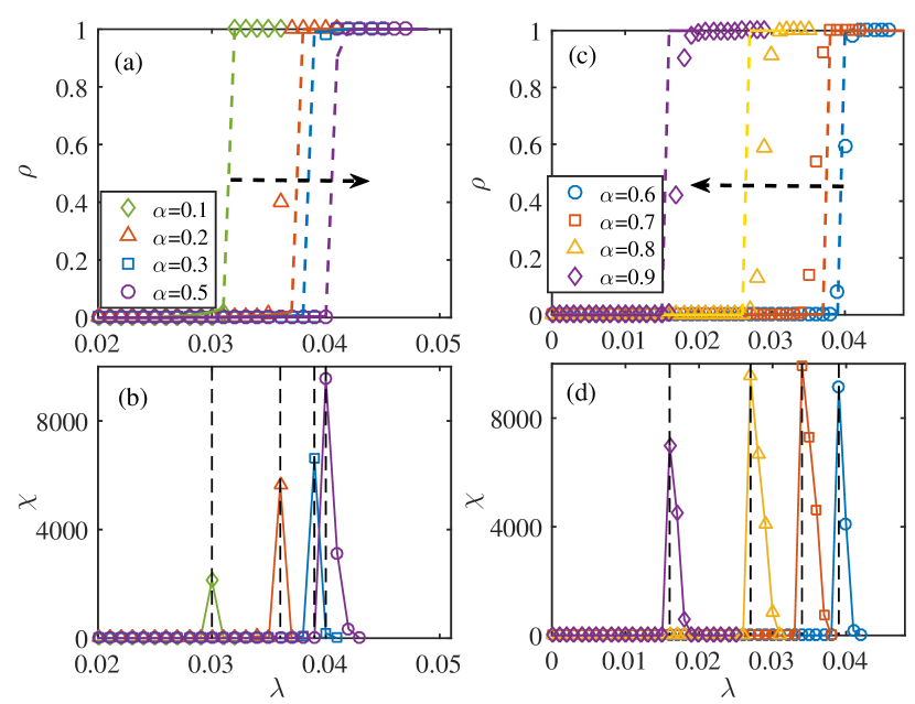
Figure 1: Effects of behavior response on the dynamics of disease spreading on a scale-free network. (a) and (c): The prevalence $\rho$ in stationary state as a function of basic infection rate $\lambda$ for varieties of reaction strength $\alpha$. Symbols represent the results obtained from Monte Carlo simulations, and lines represent the results of the GDMP method. (b) and (d): The corresponding susceptibility measure $\chi$ as a function of $\lambda$. Data are obtained by averaging over 500 independent simulations.

We first investigate the effects of behavior response on the spreading dynamics using Monte Carlo simulations. Initially, a fraction of $\rho(0)=0.1$ nodes are selected randomly as seeds, the remain nodes are in susceptible state. To present different reaction strength of individuals when they are aware of a certain disease from local information, we select eight typical values of $\alpha$ from $\alpha=0.1$ to $\alpha=0.9$ in the simulation. In Figs. 1 (a) and (c), we plot the prevalence $\rho$ in the stationary state as a function of basic infection rate $\lambda$ for different $\alpha$. Symbols in Figs. 1 (a) and (c) represent the results obtained by Monte Carlo simulations and lines are the theoretical results obtained from numeric iterations, respectively. From the curves Figs. 1(a) and (c), we observe that the system converges to two possible stationary states: either the whole population is healthy, or it becomes completely infected for any $\alpha$, which tells us that when there is a shortage in resource, the disease will break out abruptly.

Besides we can observe from Figs. 1(a) and (b) that with the increase of $\alpha$ from $\alpha=0.1$ to $\alpha=0.5$, the epidemic threshold increases gradually, see the peaks of $\chi$ for the corresponding $\alpha$. It reveals that the stronger the individual’s sense of self-protection, the more delayed the outbreak of the disease within this parameter interval (see the right arrow). On the contrary, we observe from Figs. 1(c) and (d) that when $\alpha$ increases from $\alpha=0.6$ to $\alpha=0.9$, the threshold decreases gradually, which reveals that the disease breaks out more easily with a stronger sense of self-protection within this parameter interval (see the left arrow). The phenomenon suggests that too cautious or too selfless for the people during the outbreak of an epidemic are both not suitable for disease control, and there is an optimal value of the reaction strength, at which an epidemic outbreak will be postponed to the greatest extent.

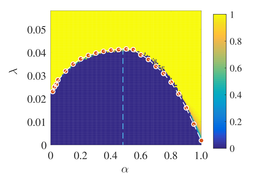
Figure 2: The phase diagram in parameter plane $(\alpha-\lambda)$ on scale-free network. Colors encode the value of $\rho$ obtained from Monte Carlo simulations. Red circles connected by dotted lines represent theoretical predictions of epidemic threshold $\lambda_{c}$. The blue dotted line indicates the location of optimal value $\alpha_{opt}$. Data are obtained by averaging 50 Monte Carlo simulations for each point in the grid $200\times 200$

We further study systematically the effects of behavior response and basic infection rate on the spreading dynamics. In Fig. 2, we exhibit the full phase diagram $(\alpha-\lambda)$ of the coupled dynamics of resource allocation and disease spreading. Colors in Fig. 2 (a) encode the fraction of infected nodes in the stationary state $\rho$. The epidemic threshold $\lambda_{c}$, marked by red circles, rises monotonically until it reaches the maximum at $\alpha_{opt}$ (indicated by the blue dotted line), and then falls gradually with the increase of $\alpha$. Besides, we observe that there are only two possible stationary state: the whole healthy (marked by blue color) and the whole infected of the population (marked by yellow color),

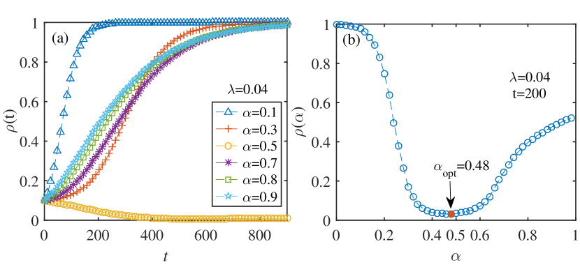
Figure 3: Effects of behavior response on evolution of the fraction of infected nodes $\rho(t)$. (a) The time evolution of $\rho(t)$ for varieties of $\alpha$ using Monte Carlo simulations for a fixed value of $\lambda=0.04$. (b) Plot of the fraction of infected nodes versus the change in $\alpha$ at a fixed time $t=200$ and infection rate $\lambda=0.04$. The results of the simulations are obtained by averaging over 300 realizations.

Fig. 3 (a) plots the time evolution of $\rho(t)$ for six typical values of $\alpha$ when the basic infection rate is fixed at $\lambda=0.04$. We find that when the value of $\alpha$ is small, the system to converge to a stationary state rapidly, such as $\rho(\infty)=1.0$ for $\alpha=0.1$. With the increase of $\alpha$, it takes a longer time for the system to reach a stationary state. Further, to exhibit the effects of $\alpha$ on the dynamics more intuitively, we plot the fraction of infected nodes at a fixed time $t=200$ as a function of $\alpha$ in Fig. 3 (b), which is denoted as $\rho(\alpha)$ for the sake of clarity. We observe that the value of $\rho(\alpha)$ decreases continuously with $\alpha$ until reaching the minimum value at $\alpha_{opt}\approx 0.48$ (marked by red circle in Fig. 3(b)), and then increases gradually with $\alpha$.

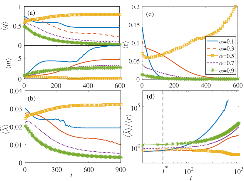
Figure 4: Plots of the critical parameters versus $t$ for typical values of $\alpha$. (a) Top pane: Time evolution of average donation rate $\langle{q}\rangle$. Bottom pane: The evolution of average number of infected neighbors of all nodes $\langle{m}\rangle$. (b) Time evolution of average infection rate $\langle{\widetilde{\lambda}}\rangle$. (c) The complete evolution of average recovery rate $\langle{r}\rangle$. (d) Log-log plots of average effective infection rate $\langle{\widetilde{\lambda}}\rangle/\langle{r}\rangle$. basic infection rate is fixed at $\lambda=0.04$. The results of the simulations are obtained by averaging over 300 realizations

Next we qualitatively explain the optimal phenomena by studying the time evolution of the critical quantities.

We begin by studying the case when $\alpha$ is small, for example, $\alpha=0.1$. We observe in Fig. 4 that in the initial stage, the donation probability for $\alpha=0.1$ is the highest [see the blue line in the top panel of Fig. 4 (a)], since a smaller value of $\alpha$ means a higher willingness of healthy individuals to allocate resources. Although the resource of healthy individuals can improve the recovery probability of infected neighbors to a certain extent, it also makes themselves more likely to be infected. We can observe in Figs. 4 (b) and (c) that, the average recovery rate $\langle{r}\rangle$ and infection rate $\langle{\widetilde{\lambda}}\rangle$ is highest for $\alpha=0.1$, meanwhile, there is a lowest value of effective infection rate $\langle{\widetilde{\lambda}}\rangle/\langle{r}\rangle$, as shown in Fig. 4 (d). However, as the high probability of being infected for the healthy nodes, the number of infected individuals increases at a high rate [see the blue line in the bottom pane of Fig. 4 (a)]. When people are aware of the increment of the infected neighbors, they will reduce their donation willingness, which leads to a reduction in infection rate $\langle{\widetilde{\lambda}}\rangle$, as shown in Figs. 4 (a) and (b). Consequently, with less resource received from healthy neighbors, the recovery rate of infected nodes reduces accordingly, see Fig. 4 (c), which leads to an increase of the effective infection rate $\langle{\widetilde{\lambda}}\rangle/\langle{r}\rangle$ Pastor-Satorras et al. (2015). The increase in $\langle{\widetilde{\lambda}}\rangle/\langle{r}\rangle$ has led to a further increase in the number of infected nodes. Then people become more aware of the threat of disease, and thus reduce the probability of resource donation further, which leads to a further decrease in infection rate $\langle{\widetilde{\lambda}}\rangle$ and recovery rate $\langle{r}\rangle$ and finally, the increase of the effective infection rate $\langle{\widetilde{\lambda}}\rangle/\langle{r}\rangle$.

Specifically, we observe from Fig. 4 (d) that, when it surpasses a critical time $t^{*}$, indicated by the dotted line in the figure, the value of $\langle{\widetilde{\lambda}}\rangle/\langle{r}\rangle$ proliferates, which suggests that in this stage the infection of healthy individuals is much faster than the recovery of infected individuals. With more newly infected nodes, the donation probability $\langle{q}\rangle$ and infection rate $\langle{\widetilde{\lambda}}\rangle$ decreases further, which results in less resources donated to support the recovery of infected nodes. Thus the recovery rate of infected nodes $\langle{r}\rangle$ drops abruptly, which in turn promotes the increases of effective infection rate $\langle{\widetilde{\lambda}}\rangle/\langle{r}\rangle$ further, and then more and number of infected nodes appear. Consequently, the cascading failure of the entire system occurs.

Based on the above analysis for a small value of $\alpha$, i.e., $\alpha=0.1$, we can reasonably explain why people are more willing to contribute a resource while the disease is more likely to break out.

Secondly, we study the case when $\alpha$ is significant, for example, $\alpha=0.9$. As a larger value of $\alpha$ means more sensitive of the individuals to the disease and a lower willingness to allocate resources. Thus we observe from Fig. 4 (a) that, initially, there is a smallest value of $\langle{q}\rangle$ [see the green stars in top pane of Fig. 4 (a)], and infection rate $\langle{\widetilde{\lambda}}\rangle$. Consequently, the infected nodes will receive the lowest value of the resource to recover, which leading to the smallest value of recovery rate $\langle{r}\rangle$, as shown the green stars in of Fig. 4 (c). Then the recovery of infected nodes is delayed leading to a high effective infection rate. We can observe in Fig. 4 (d) that, when $\alpha=0.9$, there is a highest value of $\langle{\widetilde{\lambda}}\rangle/\langle{r}\rangle$. The high effective infection rate will lead to a rapid increase in the number of infected nodes. We can observe in the bottom pane of Fig. 4 (a) that, in the early stage, there is a second largest value of $\langle{m}\rangle$ for $\alpha=0.9$, as denoted by the green stars. The large value of $\langle{m}\rangle$ will further, reduce the willingness of resource donation for the healthy individuals, thus we can observe a continuous decline in $\langle{q}\rangle$ and $\langle{\widetilde{\lambda}}\rangle$. What’s worse, the recovery rate of infected nodes keeps declining with less and less resource [see the curve in Fig. 4 (c)], which leading to a rapid growth of $\langle{\widetilde{\lambda}}\rangle/\langle{r}\rangle$ [see the curve in Fig. 4 (d)].

Thus we can explain the reason why a higher sense of self-protection of the population can not suppress the disease effectively.

At last, we observe in Fig. 4 that, when the value of $\alpha$ is around the optimal value $\alpha_{opt}$, there is a relatively lower value of $\langle{q}\rangle$ comparing to the case of $\alpha=0.1$ in the initial stage, which results in a lower value of $\langle{\widetilde{\lambda}}\rangle$ [see the yellow squares in Figs 4 (a) and (b)]. The lower willingness of resource donation induces to a relatively smaller value of recovery rate $\langle{r}\rangle$, as shown in Fig. 4 (c). However, we can observe from Fig. 4 (d) that the effective infection rate $\langle{\widetilde{\lambda}}\rangle/\langle{r}\rangle$ keeps the lowest value in the early stage, which suggests that the disease will propagate slowly in the population, and the number of infected nodes will increase slowly, which is verified by the curve in the bottom pane of Fig. 4 (a). Further, the small value of $\langle{m}\rangle$ will promotes the increase of $\langle{q}\rangle$ [see the curve in the top pane of Fig. 4 (a)], which resulting in the increase of recovery rate $\langle{r}\rangle$. And finally, the effective infection rate $\langle{\widetilde{\lambda}}\rangle/\langle{r}\rangle$ decreases further, as shown in Fig. 4 (d). Thus the disease can be suppressed to the greatest extend.

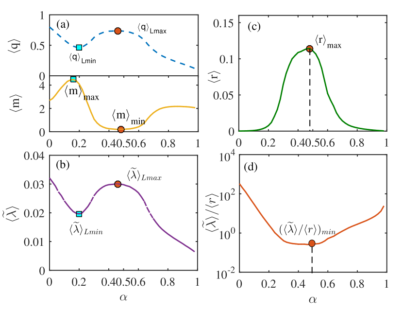
Figure 5: Plots of the critical parameters versus $\alpha$ at fixed time $t=200$ , and basic infection rate $\lambda=0.04$. (a) Top pane: the average donation rate $\langle{q}\rangle$ as a function of $\alpha$. Bottom pane: The average number of infected neighbors of all nodes $\langle{m}\rangle$ as a function of $\alpha$. (b) Average infection rate $\langle{\widetilde{\lambda}}\rangle$ as a function of $\alpha$. (c) The average recovery rate $\langle{r}\rangle$ as a function of $\alpha$. (d) Plots of average effective infection rate $\langle{\widetilde{\lambda}}\rangle/\langle{r}\rangle$. as a function of $\alpha$. The results of the simulations are obtained by averaging over 300 realizations

Through the three steps, we explain the optimal phenomena in the coupled dynamics of resource allocation and disease spreading.

Finally, we further verify our explanation by studying the critical quantities as the function of parameter $\alpha$ at a fixed time $t$ and basic infection rate $\lambda$. Figs. 5 (a) to (d) plot the value of $\langle{q}\rangle$, $\langle{m}\rangle$, $\langle{\widetilde{\lambda}}\rangle$, $\langle{r}\rangle$ and $\langle{\widetilde{\lambda}}\rangle/\langle{r}\rangle$ as a function of $\alpha$ when $t=200$, and $\lambda=0.04$. For the sake of clarity, we denote the local minimum and maximum value as $X_{Lmin}$, $X_{max}$, and the global minimum and maximum value as $X_{min}$ and $X_{max}$ respectively, where $X\in[\langle{q}\rangle,\langle{m}\rangle,\langle{\widetilde{\lambda}}\rangle,\langle{\widetilde{\lambda}}\rangle/\langle{r}\rangle]$. We observe that, although when $\alpha$ is around $\alpha_{opt}$, there is a local maximum of $\langle{q}\rangle_{Lmax}$ and $\langle{\widetilde{\lambda}}\rangle_{Lmax}$. The recovery rate reaches maximum $\langle{q}\rangle_{max}$, and the effective infection rate reaches lowest $(\langle{\widetilde{\lambda}}\rangle/\langle{r}\rangle)_{min}$, which indicates that the disease can be optimally suppressed at this point.

IV.2 Effects of network structure on coupled dynamics

In this section, we investigate the effects of network structure on the coupled dynamics of resource allocation and disease spreading. To avoid the impact of reaction strength on the result, the parameter $\alpha$ is fixed at $\alpha=0.5$. In addition, we adopt the UCM model to generate scale-free networks with different degree distributions $P(k)\sim{k}^{-\gamma}$. As the degree heterogeneity decreases with the increase of the power exponent $\gamma$ Boccaletti et al. (2006); Newman (2010), thus it approaches to random regular networks $RRNs$ when $\gamma\rightarrow{\infty}$ Chen et al. (2018a).

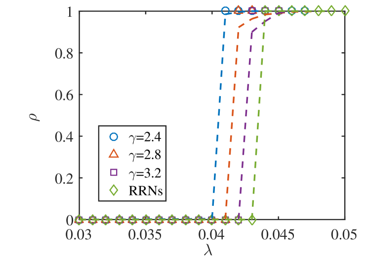
Figure 6: The prevalence $\rho$ in the stationary as a function of $\lambda$ on scale-free networks with degree exponent $\gamma=2.4$ (blue circles), $\gamma=2.8$ and $\gamma=3.2$ (purple squares). And the result on random regular network (RRNs) marked by red rhombus. Symbols represent the results obtained from Monte Carlo simulations, and lines represent results of GDMP method. The parameter $\alpha$ is fixed at $\alpha=0.5$

Fig. 6 plots the prevalence $\rho$ in the stationary state as a function of the basic infection rate $\gamma$ for networks with four typical values of $\gamma$: $\gamma=2.4$ (blue circles), $\gamma=2.8$ (upper triangles), $\gamma=3.2$ (purple squares) and $\gamma\rightarrow\infty$ (red rhombus). We observe that there are only two stationary states of the system: all healthy or completely infected for all networks, which implies that the network structure does not alter the first-order transition of $\rho$. Besides, we find that, with an increase of $\gamma$, the outbreak of disease is delayed gradually. It suggests that the degree heterogeneity enhance the disease spreading, which is consistent with the existing research conclusions Pastor-Satorras and Vespignani (2001).

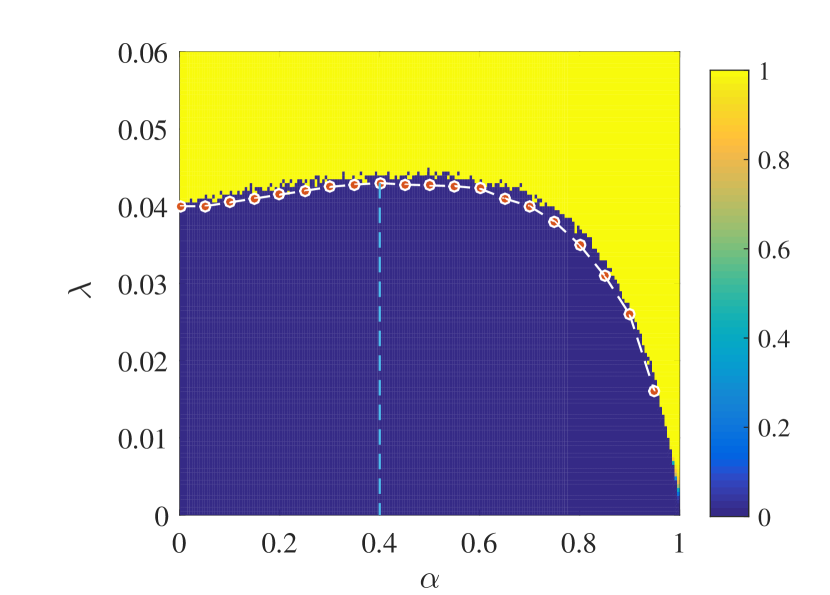
Figure 7: The phase diagram in parameter plane $(\alpha-\lambda)$ on RRNs. Colors encode the value of $\rho$ obtained from Monte Carlo simulations. Red circles connected by dotted lines represent theoretical predictions of epidemic threshold $\lambda_{c}$. The blue dotted line indicates the location of optimal value $\alpha_{opt}$. Data are obtained by averaging 50 Monte Carlo simulations for each point in the grid $200\times 200$

In the end, we study the effects of behavior response on the spreading dynamics on the spreading dynamics systematically. Fig. 7 is the phase diagram in parameter plane $(\alpha-\lambda)$ on RRNs. Colors encode the prevalence in the stationary state $\rho$. We find that there is also an optimal value $\alpha_{opt}$, at which the epidemic threshold reaches the maximum, indicated by the blue dotted line if Fig. 7. The results suggest that the network structure does not alert the optimal phenomenon in behavior response.

V Discussion

In this paper, we focus on the problem of how can we protect ourselves from being infected while helping others by donating resources during an outbreak of an epidemic. To answer this question, we propose a novel resource allocation model in controlling the epidemic spreading. We consider that healthy individual can contribute their resources to help those in need, and some will consider self-protection first when they perceive the threat of disease. The others will contribute to resource as much as possible. To quantify the behavior response of individuals, a tune parameter $\alpha$ is introduced. Besides, to study the coupled dynamics of resource allocation and disease spreading, a resource-based SIS model is proposed. First of all, we theoretically analyze the model using a generated dynamic message-passing method, and then we carry out extensive Monte Carlo simulations on both scale-free and random regular networks. Through theoretical analysis and simulations, we find that the coupled dynamics converges to two stationary states: the whole infected or all healthy, which indicates that a shortage of resource can induce an abrupt outbreak of the epidemic. More importantly, we find that too cautious or too selfless for the people during the outbreak of an epidemic are both not suitable for disease control. There is an optimal (balance) point where the epidemic spreading can be controlled to the greatest extent. It also tells us that we can donate resource appropriately to support the people in need, but at the same time, we should keep some resources for self-protection. Further, we find out the optimal point on both in certain conditions. At last, we investigate the effects of network structure on the coupled dynamics. We find that the degree heterogeneity promotes the outbreak of disease, and the network structure does not alter the optimal phenomenon in behavior response.

The discovery of the optimal (balance) point is of practical significance for controlling the outbreak of infectious diseases, especially in the context of the outbreak of 2019-ncov, in Wuhan, China. It will guide us to make the most reasonable choice between resource contribution and self-protection when perceiving the threat of disease.

VI Acknowledgements

This work was supported by the Fundamental Research Funds for the Central Universities (Nos. JBK190972, JBK171113, JBK170505), National Natural Science Foundation of China (Nos.61903266,71671141,71873108), the Financial Intelligence & Financial Engineering Key Lab of Sichuan Province, and China Postdoc-toral Science Foundation (No. 2018M631073), China Postdoctoral Science Special Foundation (No. 2019T120829).

References

References

- Chan et al. (2003) K. H. Chan, P. H. Li, S. Y. Tan, Q. Chang, and J. P. Xie, Lancet 362, 1353 (2003).
- Girard et al. (2010) M. P. Girard, J. S. Tam, O. M. Assossou, and M. P. Kieny, Vaccine 28, 4895 (2010).
- Team (2014) W. E. R. Team, New England Journal of Medicine 371, 1481 (2014).
- (4) H. emergency office National Health Commission of the People’s Republic of China, “An update on the pneumonia outbreak of novel coronavirus infection,” http://www.nhc.gov.cn/.
- Wan et al. (2008) Y. Wan, S. Roy, and A. Saberi, IET Systems Biology 2, 184 (2008).
- Gourdin et al. (2011) E. Gourdin, J. Omic, and P. Van Mieghem, in 2011 8th International Workshop on the Design of Reliable Communication Networks (DRCN) (IEEE, 2011) pp. 86–93.
- Lokhov and Saad (2017) A. Y. Lokhov and D. Saad, Proceedings of the National Academy of Sciences 114, E8138 (2017).
- Zhao et al. (2018) D. Zhao, L. Wang, Z. Wang, and G. Xiao, IEEE Transactions on Information Forensics and Security 14, 1755 (2018).
- Li et al. (2020) S. Li, D. Zhao, X. Wu, Z. Tian, A. Li, and Z. Wang, Applied Mathematics and Computation 366, 124728 (2020).
- Preciado et al. (2013) V. M. Preciado, M. Zargham, C. Enyioha, A. Jadbabaie, and G. Pappas, in 52nd IEEE Conference on Decision and Control (IEEE, 2013) pp. 7486–7491.
- Preciado et al. (2014) V. M. Preciado, M. Zargham, C. Enyioha, A. Jadbabaie, and G. J. Pappas, IEEE Transactions on Control of Network Systems 1, 99 (2014).
- Chen et al. (2017) H. Chen, G. Li, H. Zhang, and Z. Hou, Physical Review E 96, 012321 (2017).
- Granell et al. (2013) C. Granell, S. Gómez, and A. Arenas, Physical review letters 111, 128701 (2013).
- Pastor-Satorras et al. (2015) R. Pastor-Satorras, C. Castellano, P. Van Mieghem, and A. Vespignani, Reviews of Modern Physics 87, 925 (2015).
- Wang et al. (2019) W. Wang, Q.-H. Liu, J. Liang, Y. Hu, and T. Zhou, Physics Reports (2019).
- Böttcher et al. (2015) L. Böttcher, O. Woolley-Meza, N. A. Araújo, H. J. Herrmann, and D. Helbing, Scientific Reports 5, 16571 (2015).
- Chen et al. (2018a) X. Chen, R. Wang, M. Tang, S. Cai, H. E. Stanley, and L. A. Braunstein, New Journal of Physics 20, 013007 (2018a).
- Chen et al. (2018b) X. Chen, W. Wang, S. Cai, H. E. Stanley, and L. A. Braunstein, Journal of Statistical Mechanics: Theory and Experiment 2018, 053501 (2018b).
- Funk et al. (2010a) S. Funk, E. Gilad, and V. Jansen, Journal of theoretical biology 264, 501 (2010a).
- Wu et al. (2012) Q. Wu, X. Fu, M. Small, and X.-J. Xu, Chaos: an interdisciplinary journal of nonlinear science 22, 013101 (2012).
- Yang et al. (2019) H. Yang, C. Gu, M. Tang, S.-M. Cai, and Y.-C. Lai, Applied Mathematical Modelling 75, 806 (2019).
- Wang et al. (2016) W. Wang, Q.-H. Liu, S.-M. Cai, M. Tang, L. A. Braunstein, and H. E. Stanley, Scientific reports 6 (2016).
- Kulik and Mahler (1989) J. A. Kulik and H. I. Mahler, Health Psychology 8, 221 (1989).
- Nausheen et al. (2009) B. Nausheen, Y. Gidron, R. Peveler, and R. Moss-Morris, Journal of psychosomatic research 67, 403 (2009).
- Mackie et al. (2007) A. S. Mackie, L. Pilote, R. Ionescu-Ittu, E. Rahme, and A. J. Marelli, The American journal of cardiology 99, 839 (2007).
- Jaarsma et al. (1999) T. Jaarsma, R. Halfens, H. Huijer Abu-Saad, K. Dracup, T. Gorgels, J. Van Ree, and J. Stappers, European heart journal 20, 673 (1999).
- Gul and Guneri (2012) M. Gul and A. F. Guneri, International Journal of Industrial Engineering 19, 221 (2012).
- Funk et al. (2010b) S. Funk, M. Salathé, and V. A. Jansen, Journal of the Royal Society Interface 7, 1247 (2010b).
- Wang et al. (2015a) W. Wang, M. Tang, H.-F. Zhang, and Y.-C. Lai, Physical Review E 92, 012820 (2015a).
- Funk et al. (2009) S. Funk, E. Gilad, C. Watkins, and V. A. Jansen, Proceedings of the National Academy of Sciences 106, 6872 (2009).
- Karrer and Newman (2010) B. Karrer and M. E. Newman, Physical Review E 82, 016101 (2010).
- Shrestha et al. (2015) M. Shrestha, S. V. Scarpino, and C. Moore, Physical Review E 92, 022821 (2015).
- Gómez et al. (2010) S. Gómez, A. Arenas, J. Borge-Holthoefer, S. Meloni, and Y. Moreno, EPL (Europhysics Letters) 89, 38009 (2010).
- Krzakala et al. (2013) F. Krzakala, C. Moore, E. Mossel, J. Neeman, A. Sly, L. Zdeborová, and P. Zhang, Proceedings of the National Academy of Sciences 110, 20935 (2013).
- Wang et al. (2017) W. Wang, M. Tang, H. E. Stanley, and L. A. Braunstein, Reports on Progress in Physics 80, 036603 (2017).
- Schönfisch and de Roos (1999) B. Schönfisch and A. de Roos, BioSystems 51, 123 (1999).
- Wang et al. (2015b) W. Wang, P. Shu, Y.-X. Zhu, M. Tang, and Y.-C. Zhang, Chaos: An Interdisciplinary Journal of Nonlinear Science 25, 103102 (2015b).
- Girvan and Newman (2002) M. Girvan and M. E. Newman, Proceedings of the national academy of sciences 99, 7821 (2002).
- Holme and Kim (2002) P. Holme and B. J. Kim, Physical review E 65, 026107 (2002).
- Small et al. (2015) M. Small, Y. Li, T. Stemler, and K. Judd, Physical Review E 91, 042801 (2015).
- Liu et al. (2003) Z. Liu, Y.-C. Lai, and N. Ye, Physical Review E 67, 031911 (2003).
- Molloy and Reed (1995) M. Molloy and B. Reed, Random structures & algorithms 6, 161 (1995).
- Catanzaro et al. (2005) M. Catanzaro, M. Boguñá, and R. Pastor-Satorras, Physical Review E 71, 027103 (2005).
- Boguná et al. (2004) M. Boguná, R. Pastor-Satorras, and A. Vespignani, The European Physical Journal B-Condensed Matter and Complex Systems 38, 205 (2004).
- Ferreira et al. (2012) S. C. Ferreira, C. Castellano, and R. Pastor-Satorras, Physical Review E 86, 041125 (2012).
- Chen et al. (2016) X. Chen, C. Yang, L. Zhong, and M. Tang, Chaos: An Interdisciplinary Journal of Nonlinear Science 26, 083114 (2016).
- Boccaletti et al. (2006) S. Boccaletti, V. Latora, Y. Moreno, M. Chavez, and D.-U. Hwang, Physics reports 424, 175 (2006).
- Newman (2010) M. Newman, Networks: an introduction (Oxford university press, 2010).
- Pastor-Satorras and Vespignani (2001) R. Pastor-Satorras and A. Vespignani, Physical Review Letters 86, 3200 (2001).