The continuing search for evidence of tidal orbital decay of hot Jupiters

Abstract

Many of the known hot Jupiters are formally unstable to tidal orbital decay. The only hot Jupiter for which orbital decay has been directly detected is WASP-12, for which transit timing measurements spanning more than a decade have revealed that the orbital period is decreasing at a rate of $dP/dt\approx 10^{-9}$, corresponding to a reduced tidal quality factor of about $2\times 10^{5}$. Here, we present a compilation of transit-timing data for WASP-12 and eleven other systems which are especially favorable for detecting orbital decay: KELT-16; WASP-18, 19, 43, 72, 103, 114, and 122; HAT-P-23; HATS-18; and OGLE-TR-56. For most of these systems we present new data that extend the time baseline over which observations have been performed. None of the systems besides WASP-12 displays convincing evidence for period changes, with typical upper limits on $dP/dt$ on the order of $10^{-9}$ or $10^{-10}$, and lower limits on the reduced tidal quality factor on the order of $10^{5}$. One possible exception is WASP-19, which shows a statistically significant trend, although it may be a spurious effect of starspot activity. Further observations are encouraged.

1 Introduction

The discovery of 51 Pegasi b, the first known hot Jupiter, was announced nearly a quarter of a century ago (Mayor & Queloz, 1995). Now, there are several hundred confirmed hot Jupiters listed in the NASA Exoplanet Archive. Many questions remain unanswered about how these short-period gas giants formed and came to occupy orbits so close to their host stars (Dawson & Johnson, 2018).

The future of these planets is also uncertain. Theoretically, it is straightforward to show that the orbits of many of the known hot Jupiters should be slowly shrinking, due to tidal interactions between the star and planet, and the accompanying long-term dissipation of energy and transfer of angular momentum from the orbit to the star (Rasio et al., 1996; Sasselov, 2003; Levrard et al., 2009). Tidal evolution should eventually lead to planet engulfment if the orbital angular momentum is too low to allow the star to achieve spin-orbit synchronization (Hut, 1980). However, the timescale of the process is unknown and difficult to calculate theoretically, because of our incomplete understanding of the physical processes by which the energy of tidal oscillations is ultimately converted into heat (Ogilvie, 2014). The dissipation rate depends on the mass and orbital period of the planet, and probably also on the interior structure of the star, e.g., whether the star has a thick convective envelope, or a convective core (Barker & Ogilvie, 2010; Essick & Weinberg, 2015; Weinberg et al., 2017).

Population studies have provided some evidence that orbital decay does occur on astrophysically relevant timescales. Some examples are the scarcity of gas giants with periods less than a day (see, e.g. Jackson et al., 2008; Hansen, 2010; Penev et al., 2012; Ogilvie, 2014), the anomalously rapid rotation of some hot-Jupiter host stars (Penev et al., 2018) and the rarity of hot Jupiters around subgiant stars (Villaver & Livio, 2009; Hansen, 2010; Schlaufman & Winn, 2013). Tidal decay might also be responsible for the lower occurrence of close-in planets around rapidly rotating stars (Teitler & Königl, 2014), or the realignment of stars and their planetary orbits (Matsakos & Königl, 2015).

The goal of the work described in this paper is to seek more direct evidence for tidal orbital decay through long-term timing of the transits of hot Jupiters. These types of observations have already led to the detection of an apparent period decrease in the WASP-12 system (Maciejewski et al., 2016; Patra et al., 2017; Yee et al., 2020). Another candidate that recently emerged is WASP-4 (Bouma et al., 2019), although in that case, the evidence is not as compelling.

This paper is organized as follows. Section 2 describes our compilation of other promising candidates for detecting orbital decay. Section 3 presents new transit-timing data for many of these systems, and Section 4 presents analyses of all the available data. Section 4 also revisits the WASP-12 system, to address a nagging concern that the apparent timing anomalies are actually systematic errors due to unmodeled starspots affecting the transit light curve. Since this type of systematic error would likely be chromatic, we undertook multicolor photometry of several transits. Section 5 summarizes the results.

2 Target Selection

For the simple and traditional model of tidal interactions in which the equilibrium tidal bulge is tilted away from the line joining the planet and star by a small and constant angle, the rate of change of the orbital period is

$$\frac{dP}{dt}=-\frac{27\pi}{2Q^{\prime}_{\star}}\left(\frac{M_{\rm p}}{M_{\star}}\right)\left(\frac{R_{\star}}{a}\right)^{5},$$ (1)

where $Q^{\prime}_{\star}$ is the “reduced tidal quality factor,” a dimensionless number quantifying the stellar tidal dissipation rate; $M_{\rm p}$ and $M_{\star}$ are the planetary and stellar masses; $R_{\star}$ is the stellar radius; and $a$ is the orbital radius. This expression is based on the assumptions that the orbit is circular, the star’s angular velocity is much smaller than the orbital angular velocity, and the tidal dissipation within the planet can be neglected. It can be obtained by applying Kepler’s third law to Equation (20) of Goldreich & Soter (1966) or Equation (12) of Ogilvie (2014).

This theory is undoubtedly oversimplified, and the dissipation by dynamical tides may be more important than the equilibrium tides. Nevertheless, the dependence on the mass ratio and the strong dependence on orbital separation are generic features of tidal theories. Therefore, to select good candidates for detecting orbital decay, we ranked the known transiting planets according to the value of $(M_{\rm p}/M_{\star})(R_{\star}/a)^{5}$, which is proportional to $dP/dt$ according to Equation (1). We restricted the sample to host stars brighter than $V=14.5$ to make observations practical with meter-class telescopes, although we made an exception for OGLE-TR-56 ($V=16.6$) because of the long time interval over which data are available. We also made a distinction between “hot” and “cool” stars, with the dividing line at $T_{\rm eff}=6000$ K. This is because tidal dissipation is expected to be more rapid in cool stars, due to their thicker outer convective envelopes — although it is worth noting that the rapidly decaying hot Jupiter WASP-12 has a host star with $T_{\rm eff}>6000$ K (Hebb et al., 2009; Torres et al., 2012; Mortier et al., 2013). Figure 1 displays the values of the key parameters $M_{\rm p}/M_{\star}$ and $a/R_{\star}$ for the known transiting planets, with hot and cool stars depicted in different colors. Some contours of constant $P/\dot{P}$ are labeled with the predicted decay timescale according to Equation 1, assuming a nominal value of $Q_{\star}^{\prime}=10^{6}$.

We decided to focus on a dozen objects: the 5 top-ranked hot stars, and the 7 top-ranked cool stars. They are circled and identified in Figure 1, and listed in Table 1. The list includes some stars that have been observed for a decade, for which we might hope to detect orbital decay in the near term, and others that were more recently discovered, for which we wanted to establish anchor points for future monitoring. We limited the sample to a dozen objects simply to keep the project manageable in scope. There are other systems that are very nearly as good that we do not describe in this paper, but that are also worth further attenton in the future: HATS-70b, WASP-167b, CoRoT-14b, WASP-173b, WASP-87b and HAT-P-7b, to name a few.

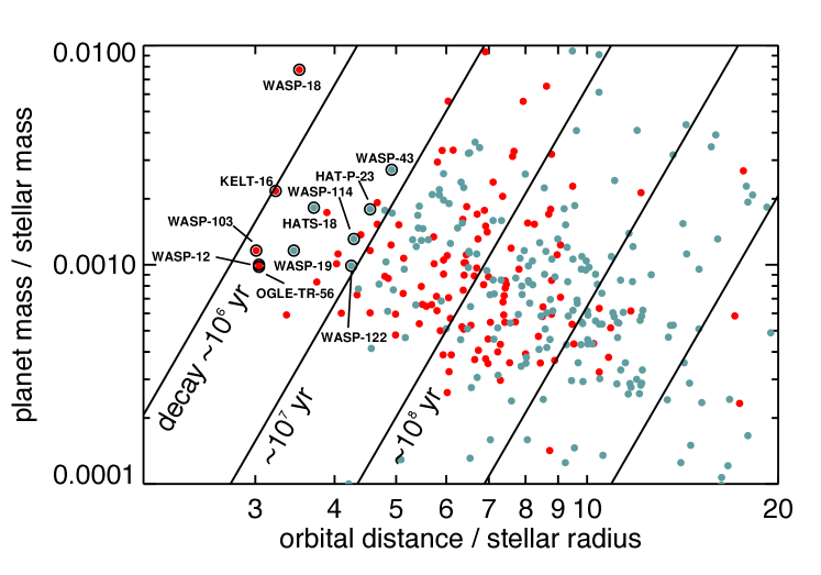
Figure 1: Key parameters for determining the rate of orbital decay. Each point represents one of the known transiting planets, with red symbols for those with “hot” host stars ($T_{\rm eff}>6000$ K) and blue symbols for those with cooler host stars. The contours of constant decay timescale are based on Equation (1) using a nominal value $Q_{\star}^{\prime}=10^{6}$. The most favorable candidates are circled and labeled.

Name	$M_{\star}/M_{\odot}$	$R_{\star}/R_{\odot}$	$T_{\rm eff}$	$M_{\rm p}/M_{\rm Jup}$	$R_{\rm p}/R_{\rm Jup}$	$a/R_{\star}$	$P$	Age	$v\sin i_{\star}$	Nobs	Figure of	Ref.
			[K]				[d]	[Gyr]	[km s-1]		merit
WASP-18	1.46(29)	1.29(05)	6431(48)	11.4(1.5)	1.20(05)	3.562(23)	0.94	1.0(0.5)	11.0(1.5)	1	16.6	1, 2, 3
KELT-16	1.211(46)	1.360(64)	6236(54)	2.75(16)	1.415(84)	3.23(13)	0.97	3.1(0.3)	7.6(0.5)	2	8.6	4
WASP-103	1.21(11)	1.416(43)	6110(160)	1.51(11)	1.623(53)	3.010(13)	0.93	4(1)	10.6(0.9)	4	6.7	5, 6
WASP-12	1.434(11)	1.657(46)	6360(140)	1.470(76)	1.900(57)	3.039(34)	1.09	2(1)	$<\,2.2$	6	5.3	7, 8
HATS-18	1.037(47)	1.020(57)	5600(120)	1.980(77)	1.34(10)	3.71(22)	0.84	4.2(2.2)	6.23(47)	2	3.6	9
WASP-19	0.935(41)	1.018(15)	5460(90)	1.139(36)	1.410(21)	3.45(14)	0.79	10.2(3.8)	4(2)	3	3.3	10, 11
OGLE-TR-56	1.228(78)	1.363(89)	6050(100)	1.39(18)	1.363(92)	3.74(19)	1.21	3.1(1.2)	3(1)	2	2.1	12, 13
HAT-P-23	1.130(35)	1.203(74)	5905(80)	2.09(11)	1.368(90)	4.14(23)	1.21	4(1)	8.1(0.5)	3	2.0	14
WASP-72	1.386(55)	1.98(24)	6250(100)	1.546(59)	1.27(20)	4.02(49)	2.22	3.2(0.6)	6.0(0.7)	2	1.4	15
WASP-43	0.717(25)	0.667(11)	4520(120)	2.034(52)	1.036(19)	4.918(53)	0.81	$\cdots$	2(1)	3	1.3	16
WASP-114	1.289(53)	1.43(60)	5940(140)	1.769(64)	1.339(64)	4.29(19)	1.55	4(2)	6.4(0.7)	1	1.3	17
WASP-122	1.239(39)	1.52(03)	5720(130)	1.284(32)	1.743(47)	4.248(72)	1.71	5.11(80)	3.3(0.8)	0	1.0	18

Table 1: Favorable targets for the search for tidal orbital decay. Parentheses enclose the uncertainties in the last few digits, e.g., 4(1) means $4\pm 1$ and 1.363(92) means $1.363\pm 0.092$. N_obs is the number of new light curves reported in this paper. The figure of merit in the second-to-last column is proportional to $(M_{\rm p}/M_{\star})(R_{\star}/a)^{5}$, and normalized to unity for WASP-122. References: 1 - Stassun et al. (2017); 2 - Shporer et al. (2019); 3 - Hellier et al. (2009); 4 - Oberst et al. (2017); 5 - Delrez et al. (2018); 6 - Gillon et al. (2014); 7 - Collins et al. (2017); 8 - Hebb et al. (2009); 9 - Penev et al. (2016); 10 - Mancini et al. (2013) 11 - Hebb et al. (2010); 12 - Torres et al. (2008); 13 - Sasselov (2003); 14 - Bakos et al. (2011); 15 - Gillon et al. (2012); 16 - Hellier et al. (2011); 17 - Barros et al. (2016); 18 - Turner et al. (2016). Notes: For WASP-18, $a/R_{\star}$ is from Ref. 2, while age and $v\sin i_{\star}$ are from Ref. 3. For WASP-103, $v\sin i_{\star}$ is from Ref. 6. For WASP-12, age and $v\sin i_{\star}$ are from Ref. 8. For WASP-19, $v\sin i_{\star}$ is from Ref. 11. For OGLE-TR-56, $v\sin i$ is from Ref. 13.

3 Observations of New transits

Transits of KELT-16b, WASP-103b, HAT-P-23b, and WASP-114b were observed with the 1.2m telescope at the Fred Lawrence Whipple Observatory (FLWO) on Mount Hopkins in Arizona. Time-series photometry was performed using images from the KeplerCam detector and a Sloan $r^{\prime}$-band filter. The field of view of this camera is $23.1$ arcmin on a side. We used $2\times 2$ binning, giving a pixel scale of $0.68$ arcsec. Transits of WASP-19b, WASP-43b, WASP-18b, WASP-72b and HATS-18 were observed with the 0.6m TRAPPIST-South telescope at Observatorio La Silla, Chile (Gillon et al., 2011; Jehin et al., 2011). TRAPPIST-South is equipped with a 2048$\times$2048 pixels FLI Proline PL3041-BB CCD camera with a field of view of $22$ arcmin on a side, giving a pixel scale of $0.64$ arcsec. Two additional transits of WASP-43b were obtained with the TRAPPIST-North telescope at the Oukaimeden Observatory, Morocco (Barkaoui et al., 2019). It is a twin telescope in the Northern hemisphere equipped with a 2000$\times$2000 deep-depletion Andor IKONL BEX2 DD CCD camera with a pixel scale of $0.60$ arcsec and an on-sky field of view of $20$ arcmin. Transits of OGLE-TR-56b were observed with the 6.5m Magellan Clay Telescope at Las Campanas Observatory in Chile. Multi-color transits of WASP-12b were observed by the MuSCAT camera on the 1.88 m telescope at the Okayama Astrophysical Observatory in Japan (Narita et al., 2015).

For transits observed before March 2018, raw images were processed by performing standard overscan correction, debiasing, and flat-fielding with IRAF. For transits observed thereafter, we used AstroImageJ [AIJ; Collins et al. (2017)] to perform these same steps. The observation time-stamps were placed on the BJD_TDB time system using the time utilities code of Eastman et al. (2010). Aperture photometry was performed for each target and an ensemble of about 8 comparison stars of similar brightness. The reference signal was generated by summing the flux of the comparison stars. The flux of the target star was then divided by this reference signal to produce a time series of relative flux. This procedure was performed for many different choices of the aperture radius, and the final radius was selected to give the smallest possible scatter in the relative flux of the target star, outside of the transits.

After each time series was normalized to have unit flux outside of the transit, we fitted a Mandel & Agol (2002) model to the data from each transit. The parameters of the transit model were the mid-transit time, the planet-to-star radius ratio ($R_{p}$/$R_{\star}$), the scaled stellar radius ($R_{\star}/a$), and the impact parameter [$b=a\cos i/R_{\star}$]. For given values of $R_{\star}/a$ and $b$, the transit timescale is proportional to the orbital period [see, e.g., Equation (19) of Winn (2010)]. To set this timescale, we held the period fixed at its most recent measurement for each target, although the individual transits were fitted separately with no requirement for periodicity. To correct for differential extinction, we allowed the apparent magnitude to be a linear function of airmass, giving two additional parameters. The limb darkening law was assumed to be quadratic, with coefficients held fixed at the values tabulated by Claret & Bloemen (2011) for each target star with its spectroscopic properties adopted from the corresponding discovery paper. To interpolate the tables, we used the online tool built by Eastman et al. (2013). To determine the credible intervals for the parameters, we used emcee, an affine invariant Markov Chain Monte Carlo (MCMC) ensemble sampler code written by Foreman-Mackey et al. (2013). The transition distribution was proportional to $\exp(-\chi^{2}/2)$ with

$$\chi^{2}=\sum_{i=1}^{N}\left(\frac{f_{{\rm obs},i}-f_{{\rm calc},i}}{\sigma_{i}}\right)^{2}$$ (2)

where $f_{{\rm obs},i}$ is the observed flux at time $t_{i}$ and $f_{{\rm calc},i}$ is the calculated flux based on the model parameters. The uncertainties $\sigma_{i}$ were set equal to the standard deviation of the out-of-transit data. In some transits, the pre-ingress scatter was noticeably different than the post-egress scatter; for those observations, we assigned $\sigma_{i}$ by linear interpolation between the pre-ingress and post-egress values. The resulting uncertainty estimates appear to be realistic, in the sense that the measured transit times within a given season generally agree to within 1-$\sigma$ with a constant period. Hence, no further allowance for time-correlated noise was made. Figures 3 through 15 show the new light curves and the best-fitting models. Table 2 presents the new transit times for all observed targets.

In addition, to extend the time baseline as far as possible, we looked for any pre-discovery transit detections in the database of the All Sky Automated Survey [ASAS; Pojmanski (1997)]. We considered only the data having a quality grade of A or B (good to average quality). We converted the time stamps from HJD_UTC to BJD_TDB using the online applet of Eastman et al. (2010). Different datasets were normalized to the same median magnitude and a “best aperture” column was produced that gave the lowest scatter. Outliers were removed by 5-$\sigma$-clipping. To retrieve the transit signal, the time-series was phase-folded using the discovery epoch and orbital period. The only case for which we detected a significant transit dip was WASP-18, shown in Figure 2. The transit was fitted with a model following an identical procedure used for other planets.

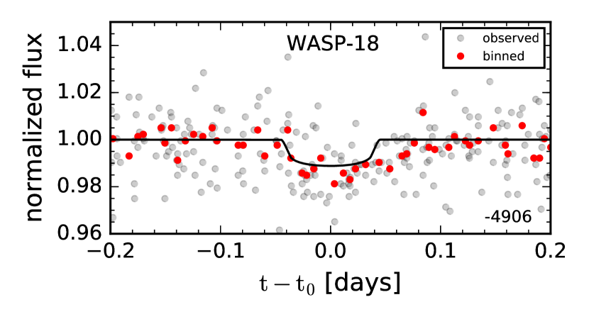
Figure 2: Pre-discovery transit light curve for WASP-18 b. Epoch number is printed to the bottom right of the frame.

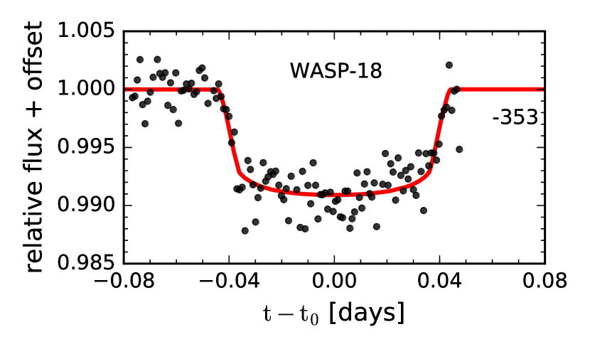
Figure 3: New transit light curve for WASP-18 b. Epoch number is printed to the bottom right of the frame.

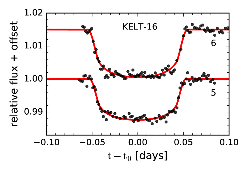
Figure 4: New transit light curves for KELT-16 b. Epoch numbers are printed to the right of each curve. Vertical offsets have been applied to separate the light curves.

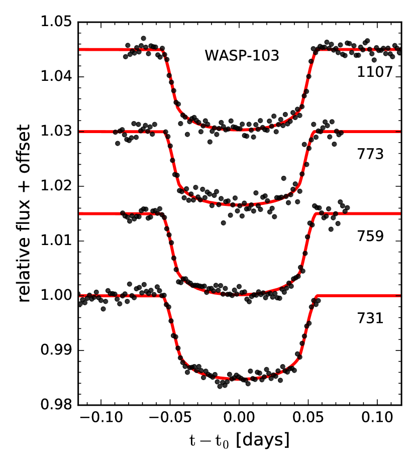
Figure 5: New transit light curves for WASP-103 b. Epoch numbers are printed to the right of each curve. Vertical offsets have been applied to separate the light curves.

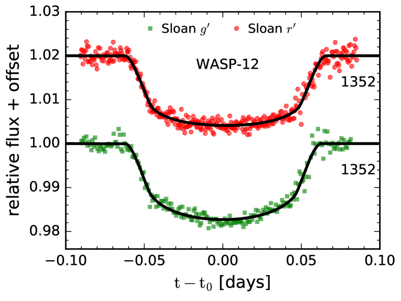
Figure 6: Multicolor light curves of WASP-12 b from epoch 1352.

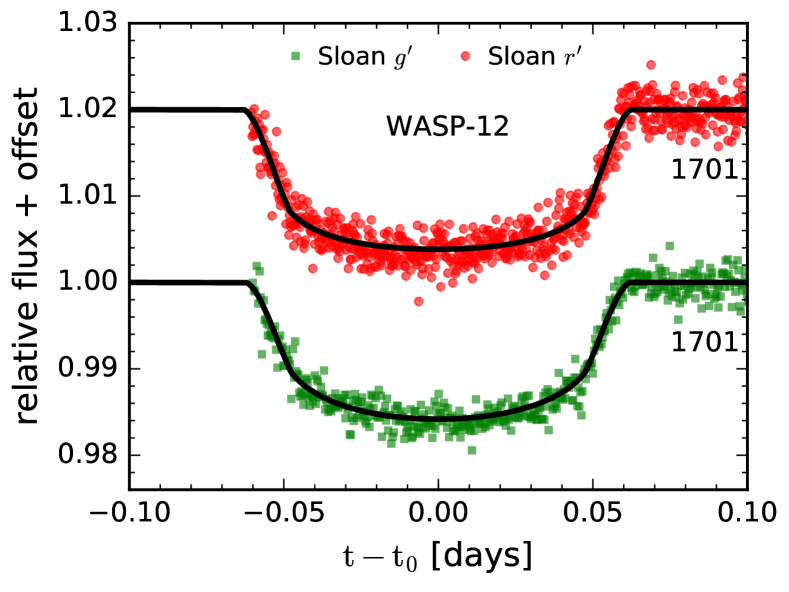
Figure 7: Multicolor light curves of WASP-12 b from epoch 1701.

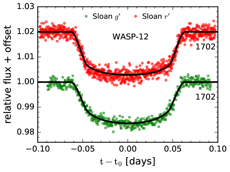
Figure 8: Multicolor light curves of WASP-12 b from epoch 1702.

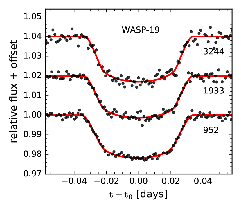
Figure 9: New transit light curves for WASP-19 b. Epoch numbers are printed to the right of each curve. Vertical offsets have been applied to separate the light curves.

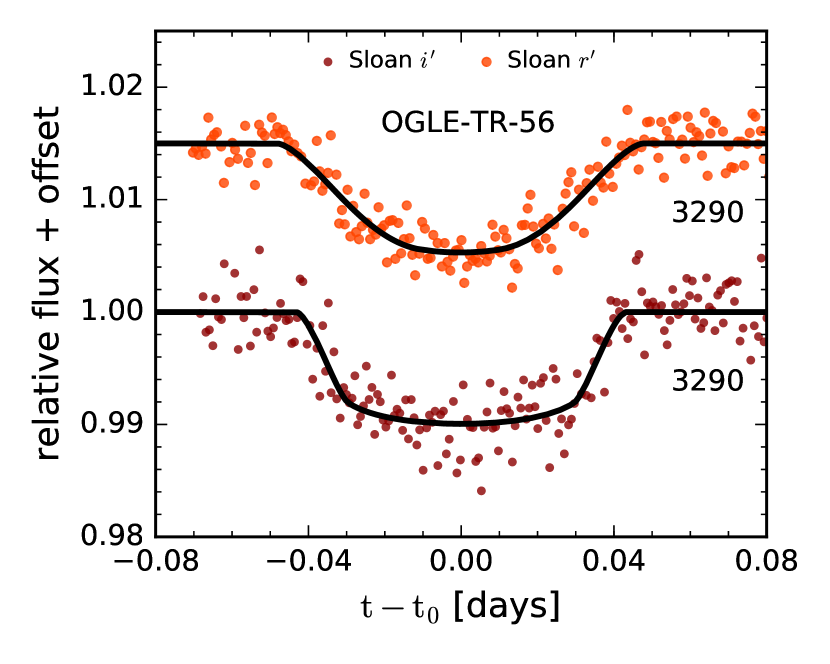
Figure 10: New transit light curves for OGLE-TR-56 b. Epoch numbers are printed to the right of each curve. Vertical offsets have been applied to separate the light curves.

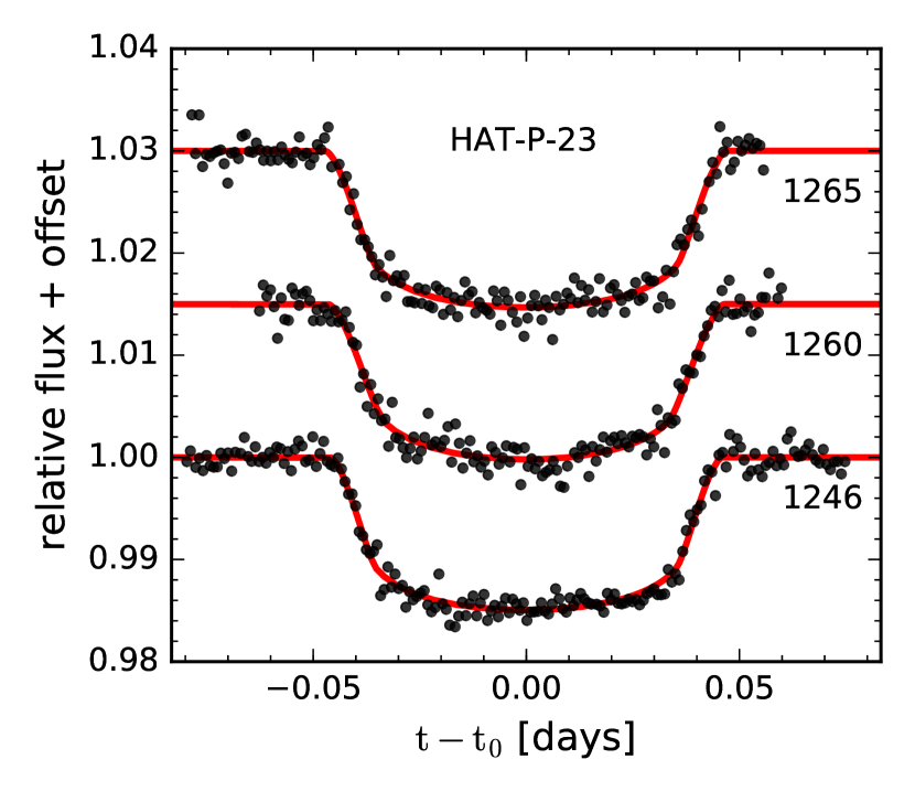
Figure 11: New transit light curves for HAT-P-23 b. Epoch numbers are printed to the right of each curve. Vertical offsets have been applied to separate the light curves.

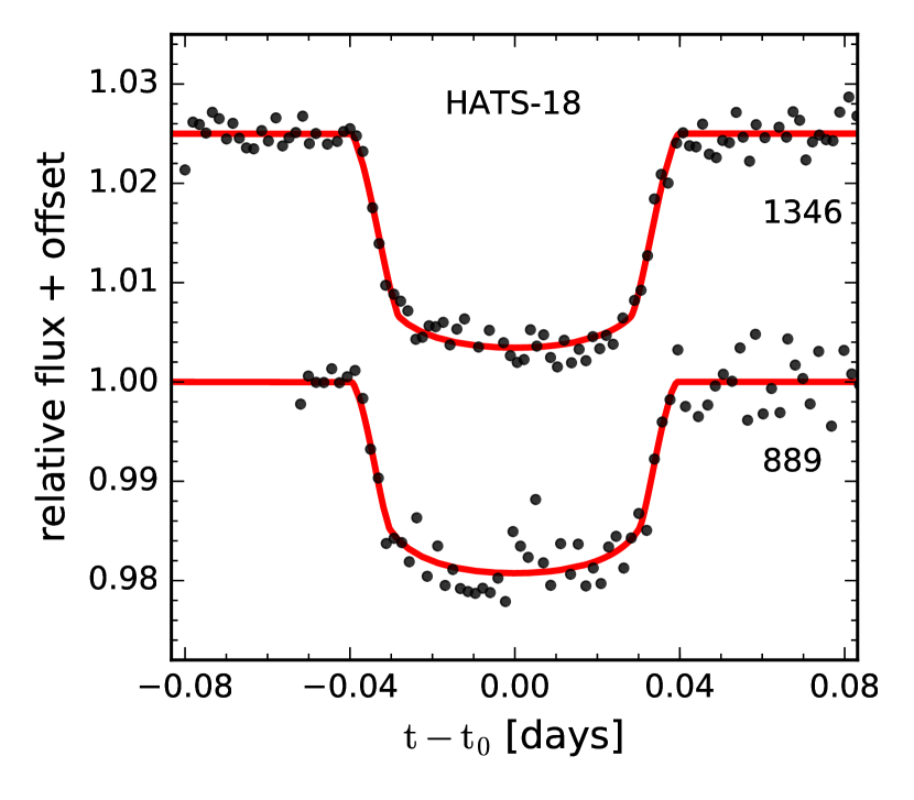
Figure 12: New transit light curves for HATS-18 b. Epoch numbers are printed to the right of each curve. Vertical offsets have been applied to separate the light curves.

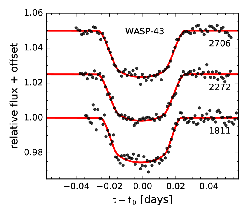
Figure 13: New transit light curves for WASP-43 b. Epoch numbers are printed to the right of each curve. Vertical offsets have been applied to separate the light curves.

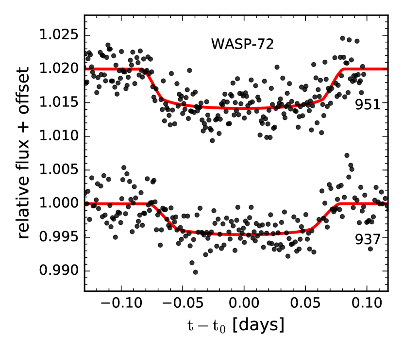
Figure 14: New transit light curves for WASP-72 b. Epoch numbers are printed to the right of each curve. Vertical offsets have been applied to separate the light curves.

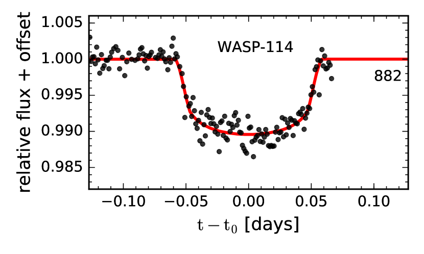
Figure 15: New transit light curve for WASP-114 b. Epoch number is printed to the right of the curve.

4 Timing Analysis

For each target, we considered all the transit times from this work as well as all the available times reported in the literature for which (i) the midpoint was allowed to be a completely free parameter in the fit to the light curve, (ii) the time system was documented clearly, and (iii) the light curve included both the ingress and the egress of the transit. For KELT-16b, WASP-103b and HAT-P-23b, in particular, we built on the study of Maciejewski et al. (2018). Apart from presenting new transits for these systems, those authors refitted the transit data drawn from the literature for the sake of homogeneity. We note that their reanalyzed times differ from the originally reported times by several minutes in some cases (see below for more details). Table 3 presents the transit times for all targets.

We fitted two models to the timing data. The first model assumes a constant orbital period:

$$t_{\rm tra}(E)=t_{0}+PE,$$ (3)

where $E$ is the epoch number and $P$ is the period. The second model assumes a constant period derivative:

$$t_{\rm tra}(E)=t_{0}+PE+\frac{1}{2}P\frac{dP}{dt}E^{2}.$$ (4)

We determined the best-fitting parameters and their uncertainties using a Markov Chain Monte Carlo (MCMC) method. Below we summarize the results for each target. In all of the figures showing the timing residuals, with the exception of WASP-114 and HATS-18, we have also plotted a band depicting the 1-$\sigma$ range of uncertainty in the orbital decay model. This region encapsulates 68% of the orbital decay solutions from the Markov chains. For WASP-114 and HATS-18, currently only two and three transit times are available respectively, so the red band in Figure 26 and 20 represents the 1-$\sigma$ range of uncertainty in the constant-period model.

Target	Date-Obs	Telescope	Filter	Exp	Epoch	Tmid	Unc
	(UTC)			(sec)		BJDTDB (days)	(days)
WASP-18 b	2005-Feb-01	ASAS	$V$	180	-4906	2453403.36480	0.00614
WASP-18 b	2016-Oct-28	TRAPPIST-South	$z^{\prime}$	7	-353	2457689.79147	0.00075
KELT-16 b	2017-June-10	FLWO	$r^{\prime}$	30	5	2457914.88456	0.00051
KELT-16 b	2017-June-11	FLWO	$r^{\prime}$	30	6	2457915.85370	0.00062
WASP-103 b	2016-May-04	FLWO	$r^{\prime}$	30	731	2457512.87006	0.00031
WASP-103 b	2016-May-30	FLWO	$r^{\prime}$	30	759	2457538.78548	0.00030
WASP-103 b	2016-Jun-12	FLWO	$r^{\prime}$	30	773	2457551.74314	0.00038
WASP-103 b	2017-Apr-17	FLWO	$r^{\prime}$	30	1107	2457860.87503	0.00029
WASP-12 b	2017-Jan-27	MuSCAT	$g^{\prime}$	30	1352	2457781.05418	0.00043
WASP-12 b	2017-Jan-27	MuSCAT	$r^{\prime}$	15	1352	2457781.05566	0.00036
WASP-12 b	2018-Feb-12	MuSCAT	$g^{\prime}$	30	1701	2458161.95991	0.00035
WASP-12 b	2018-Feb-12	MuSCAT	$r^{\prime}$	15	1701	2458161.95964	0.00026
WASP-12 b	2018-Feb-13	MuSCAT	$g^{\prime}$	30	1702	2458163.05089	0.00034
WASP-12 b	2018-Feb-13	MuSCAT	$r^{\prime}$	15	1702	2458163.05125	0.00021
WASP-19 b	2014-Apr-25	TRAPPIST-South	$I+z^{\prime}$	12	952	2456772.67789	0.00052
WASP-19 b	2016-Jun-07	TRAPPIST-South	$I+z^{\prime}$	12	1933	2457546.53025	0.00038
WASP-19 b	2019-Apr-07	TRAPPIST-South	$I+z^{\prime}$	12	3244	2458580.69724	0.00040
HAT-P-23 b	2016-Sep-09	FLWO	$r^{\prime}$	20	1246	2457640.69114	0.00046
HAT-P-23 b	2016-Sep-26	FLWO	$r^{\prime}$	20	1260	2457657.67134	0.00062
HAT-P-23 b	2016-Oct-02	FLWO	$r^{\prime}$	20	1265	2457663.73660	0.00044
WASP-72 b	2016-Sep-29	TRAPPIST-South	$I+z^{\prime}$	10	937	2457660.73274	0.00302
WASP-72 b	2016-Oct-30	TRAPPIST-South	$I+z^{\prime}$	10	951	2457691.77307	0.00250
WASP-114 b	2017-Oct-07	FLWO	$r^{\prime}$	30	882	2458033.75834	0.00068
OGLE-TR-56 b	2017-Jun-19	Magellan Clay	$r^{\prime}$	20	3290	2457923.79020	0.00091
OGLE-TR-56 b	2017-Jun-19	Magellan Clay	$i^{\prime}$	20	3290	2457923.78858	0.00108
WASP-43 b	2017-Mar-03	TRAPPIST-South	$z^{\prime}$	12	1811	2457815.54442	0.00038
WASP-43 b	2018-Mar-13	TRAPPIST-North	$I+z^{\prime}$	10	2272	2458190.55560	0.00026
WASP-43 b	2019-Mar-01	TRAPPIST-North	$z^{\prime}$	12	2706	2458543.60361	0.00027
HATS-18 b	2017-Mar-22	TRAPPIST-South	$I+z^{\prime}$	30	889	2457834.74845	0.00040
HATS-18 b	2018-Apr-09	TRAPPIST-South	$z^{\prime}$	25	1346	2458217.64370	0.00029

Table 2: Observation journal and measured mid-transit times.

Target	Epoch	Tmid (BJDTDB)	Error(days)	Reference
HAT-P-23	-1163	2454718.84863	0.000466	Bakos et al. 2011
	-1159	2454723.69918	0.000388	”
	-1117	2454774.6412	0.000555	”
	-909	2455026.92065	0.000436	”
	-341	2455715.84171	0.001013	Ramón-Fox & Sada 2013
	-290	2455777.69757	0.001314	”
	-280	2455789.82601	0.001098	”

Table 3: Transit times of all targets. This table represents the form of timing data; the complete table can be accessed from the electronic version of this work.

1. WASP-18 b is a “super-Jupiter” with a mass of 11.4 $M_{\rm Jup}$ in a 0.94-day orbit around a relatively hot F-type star (Hellier et al., 2009; Stassun et al., 2017). The planet’s mass is large enough that the system is not formally unstable to tidal decay, although the period may be shrinking as the system approaches synchronization. Wilkins et al. (2017) found no signs of orbital decay in the system over a decade. McDonald & Kerins (2018) found 1.3-$\sigma$ (i.e., weak) evidence for orbital decay when considering a pre-discovery transit observation by Hipparcos. More recently, Shporer et al. (2019) reported on observations with the Transiting Exoplanet Survey Satellite (Ricker et al., 2015), adding high-precision transit times to the existing ephemeris.

   We compiled and analyzed the available transit timing data, shown in Figure 16. The best-fitting orbital decay model gives $\frac{dP}{dt}=-(1.2\pm 1.3)\times 10^{-10}$. The evidence for orbital decay found by McDonald & Kerins (2018) has been further weakened with the inclusion of the TESS data. Due to a lack of conclusive evidence for orbital decay, we can set a 95%-confidence lower limit on $Q^{\prime}_{\star}$ of $(1.7\pm 0.4)\times 10^{6}$. Here and elsewhere, this limit was obtained by calculating the 95%-confidence limit on $dP/dt$ and then applying Equation (1) to convert it into a limit on $Q^{\prime}_{\star}$. The uncertainty of 0.4 is based on the propagation of the uncertainties in $M_{\rm p}/M_{\star}$ and $a/R_{\star}$ from Table 1.

   Our result for WASP-18 is consistent with the 2-$\sigma$ limit $Q^{\prime}_{\star}>10^{6}$ derived by Wilkins et al. (2017). The refined transit ephemeris is $t_{\rm tra}(E)=2458022.12523(02)~{}\rm{BJD_{TDB}}$ + $E\times 0.941452425(22)~{}\rm{days}$.

   

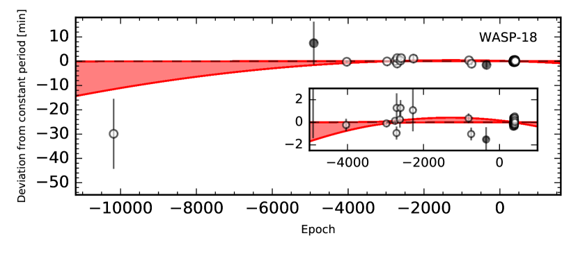
   Figure 16: Timing residuals for WASP-18 b. White points represent transit times collected from the literature: Hellier et al. (2009), Maxted et al. (2013), Wilkins et al. (2017), McDonald & Kerins (2018) and Bouma et al. (2019). The black point shows the pre-discovery transit from ASAS. The inset, with same axes units as the main frame, shows a zoomed in version of timing residuals between epochs $-5000$ and 1000. The red band represents the 1-$\sigma$ uncertainty in the orbital decay model.

2. KELT-16 b is a 2.8 $M_{\rm Jup}$ planet in a 0.97-day orbit around an F star (Oberst et al., 2017). In their follow-up study, Maciejewski et al. (2018) refitted the transits presented by Oberst et al. (2017) to redetermine transit times. Their times differ from those reported originally by about 30 seconds. In this work, we present two new transit times, which put together with times reported by Maciejewski et al. (2018) are shown in Figure 17

   

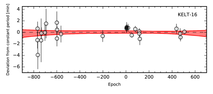
   Figure 17: Timing residuals for KELT-16b. White points represent transit times originally reported by Oberst et al. (2017) and reanalyzed by Maciejewski et al. (2018). Black points represent new data. The red band represents 1-$\sigma$ uncertainty on the orbital decay model.

   The best-fit orbital decay model results in $\frac{dP}{dt}=-(0.6\pm 1.4)\times 10^{-9}$, consistent with a constant period. The lack of a decreasing period allows us to limit the reduced tidal quality factor to $Q^{\prime}_{\star}>(0.9\pm 0.2)\times 10^{5}$ with 95% confidence. We refined the constant-period ephemeris to $t_{\rm tra}(E)=2457910.03913(11)~{}\rm{BJD_{TDB}}$ + $E\times 0.96899319(30)~{}\rm{days}$.

3. WASP-103 b is a 1.5 $M_{\rm Jup}$ planet in a 0.93-day orbit around a late F star (Gillon et al., 2014). Maciejewski et al. (2018) presented several new transit times and also reanalyzed light curves available in the literature. We present 4 new transits of WASP-103b which, along with times from Maciejewski et al. (2018), are shown in Figure 18.

   

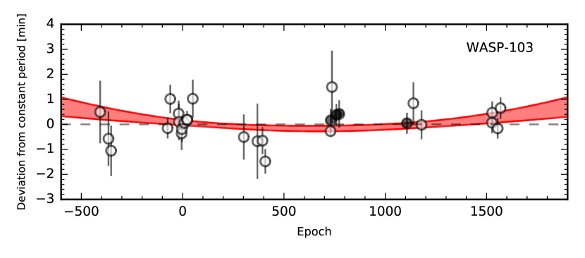
   Figure 18: Timing residuals for WASP-103 b. White points are data obtained and reanalyzed by Maciejewski et al. (2018) and originally reported by Gillon et al. (2014); Southworth et al. (2015); Delrez et al. (2018); Turner et al. (2017) and Lendl et al. (2017). Black points represent new data. The red band represents the 1-$\sigma$ uncertainty inn the orbital decay model.

   The best-fit orbital decay model results in $\frac{dP}{dt}=(8.42\pm 3.95)\times 10^{-10}$. Note the positive period derivative, which could be a statistical artifact or the sign of a period change due to some other reason (such as a third body in the system, or apsidal precession). Treating the result as a non-detection of orbital decay, we can constrain the tidal quality factor to be $Q^{\prime}_{\star}>(1.1\pm 0.1)\times 10^{5}$ with 95% confidence. We refined the linear ephemeris to $t_{\rm tra}(E)=2456836.29630(07)~{}\rm{BJD_{TDB}}$ + $E\times 0.925545352(94)~{}\rm{days}$.

4. WASP-12 b is a 1.5 $M_{\rm Jup}$ planet in 1.1-day orbit around a star that appears to be a late F main-sequence star, but could also be a subgiant (Hebb et al., 2009; Weinberg et al., 2017). Maciejewski et al. (2016) reported the first indication of a systematic quadratic deviation from a constant-period model. Patra et al. (2017) confirmed the aforementioned result and found the rate of period change to be $-29\pm 3$ ms yr^-1. The implied tidal quality factor is $Q_{\star}\approx 2\times 10^{5}$. Although both sets of authors pointed out that the available data might also be explained by the apsidal precession of the orbit, Yee et al. (2020) found that the interval between the measured times of occultations has also been shrinking, which is evidence in favor of orbital decay.

   The sky-projected obliquity of WASP-12 b has been measured to be $\lambda=59^{+15}_{-20}$ deg. The sky-projected rotation velocity $v\sin i$ is less than 2.2 km s^-1, which is unusually low for an F-type star (Albrecht et al., 2012; Hebb et al., 2009), and suggests that our line of sight may be nearly aligned with the stellar rotation axis. This made us wonder if the measured transit times are being thrown off from the true values due to stellar activity. A slowly-varying spot pattern near one of the rotation poles could lead to a persistent deformity of the transit light curve, which would manifest itself as a perturbation in the fitted transit time. A long-term activity cycle might cause this perturbation to gradually change amplitude, leading to a spurious detection of a change in orbital period. We decided to test for this effect by observing the same transit at different wavelengths. Starspot activity is generally chromatic. If the apparent transit time appears to vary with wavelength, that would be a sign of systematic errors due to stellar activity.

   We used the multicolor camera on MuSCAT to observe transits simultaneously in three different filters: $g^{\prime}$, $r^{\prime}$, and $z^{\prime}$. Transits were observed on 2017 Jan 27, 2018 Feb 12, and 2018 Feb 13, although in practice we used only the $g^{\prime}$ and $r^{\prime}$ data because of the relatively lower quality of the $z^{\prime}$ data. All the light curves were fitted independently. Along with the transit model, we also fitted for linear functions to decorrelate the apparent magnitude with the $X$ and $Y$ positions of the target star on the CCD, and on the airmass. Figures 6, 7 and 8 show the light curves and the best-fit transit models. Figure 19 shows the positions of these mid-transit times among all other timing residuals.

   

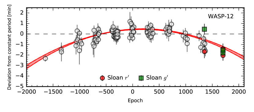
   Figure 19: Timing residuals for WASP-12 b. White points are from Hebb et al. (2009); Copperwheat et al. (2013); Chan et al. (2011); Collins et al. (2017); Maciejewski et al. (2013); Sada et al. (2012); Cowan et al. (2012); Stevenson et al. (2014); Maciejewski et al. (2016); Kreidberg et al. (2015); Patra et al. (2017). Red and green points represent new data obtained with MuSCAT. The red band represents 1-$\sigma$ uncertainty in the orbital decay model.

   For epoch 1352, the $r^{\prime}$ and $g^{\prime}$ times differ from each other by 3-$\sigma$. However, we do not ascribe too much significance to this discrepancy, because on this night there were very large transparency variations during egress and several data points had to be excluded as large outliers. The other two transits were obtained in good weather and the results show good agreement between the transit times measured in the two bands, as well as consistency with the previously established trend of a shrinking period. Thus, there is no indication that the transit timing deviations are chromatic, although we do intend to continue multicolor observations to check further.

5. HATS-18 b is a 2 $M_{\rm Jup}$ planet in a 0.84-day orbit around a G star Penev et al. (2016). Since there are only three available data points, we were not able to perform a meaningful search for period changes, although we were able to reduce the uncertainty in the orbital period by a factor of two. The up-to-date ephemeris is $t_{\rm tra}(E)=2457089.90665(25)~{}\rm{BJD_{TDB}}$ + $E\times 0.83784309(28)~{}\rm{days}$.

   

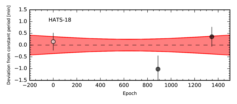
   Figure 20: Timing residuals for HATS-18 b. The white point is from Penev et al. (2016) and the black points represent new data. The red band depicts 1$\sigma$ uncertainty on the linear ephemeris.

6. WASP-19 b is the shortest-period hot Jupiter yet discovered, with a period of 0.78 days (Hebb et al., 2010). The planet has a mass of 1.1 $M_{\rm Jup}$ and orbits a star very similar to the Sun in mass. We have added 3 new transit times to the existing collection. The timing residuals are shown in Figure 21.

   

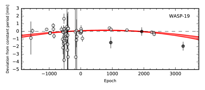
   Figure 21: Timing residuals for WASP-19 b. White points are data reported in the literature: Hebb et al. (2010); Hellier et al. (2011); Dragomir et al. (2011); Lendl et al. (2013); Tregloan-Reed et al. (2013); Mancini et al. (2013); Bean et al. (2013); Espinoza et al. (2019). Black points represent new data obtained by TRAPPIST. The red band represents 1$\sigma$ uncertainty on the orbital decay model.

   The best-fitting orbital decay model results in $\frac{dP}{dt}=-(2.06\pm 0.42)\times 10^{-10}$, equivalent to $-(6.5\pm 1.3)$ ms yr^-1. If the orbit is indeed decaying, the implied tidal quality factor is $Q^{\prime}_{\star}=(5.0\pm 1.5)\times 10^{5}$. For comparison, WASP-12 has a period derivative of $-~{}(29\pm 3)$ ms yr^-1 and a reduced tidal quality factor of $(1.6\pm 0.2)\times 10^{5}$. Formally, the period change of WASP-19 b is stastically significant. However, we are cautious because the data are relatively scanty in comparison with WASP-12 b, and there appears to be a lot of scatter. Two of our new transit times, in particular, deviate from the best-fitting model by more than 1-$\sigma$.

   Both Mancini et al. (2013) and Espinoza et al. (2019) attributed some previously noted timing inconsistencies to starspot activity. In several cases, an anomaly in the light curve was clearly detected. For this reason, we believe that further observations are required to determine if there is a indeed a departure from constant period. In the meantime, we have refined the linear ephemeris for transits to be $t_{\rm tra}(E)=2456021.70390(02)~{}\rm{BJD_{TDB}}$ + $E\times 0.788839300(17)~{}\rm{days}$.

7. OGLE-TR-56 b is the most challenging target in our list to observe because of the relatively faint star ($V$ = 16.6). On the other hand, it is one of the earliest discovered transiting exoplanets, which means that there is an unusually long time baseline over which data are available. The discovery of this planet also inspired some early attempts to model tidal orbital decay (see, e.g., Sasselov, 2003; Carone & Pätzold, 2007).

   Adams et al. (2011) performed a major transit-timing study based on 21 light curves. To this, we have added one new transit time in 2017, more than 6 years later. The timing residuals are shown in Figure 22. We do not find significant evidence for orbital decay. The best-fit orbital decay model results in $\frac{dP}{dt}=(3.34\pm 1.49)\times 10^{-10}$, a weak period increase. Treating this result as a null detection, we conclude that $Q^{\prime}_{\star}>(7.0\pm 2.1)\times 10^{5}$ with 95% confidence. The updated linear ephemeris is $t_{\rm tra}(E)=2453936.60063(14)~{}\rm{BJD_{TDB}}$ + $E\times 1.21191123(16)~{}\rm{days}$.

   

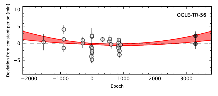
   Figure 22: Timing residuals for OGLE-TR-56 b. White points were reported by Torres et al. (2004); Pont et al. (2007) and Adams et al. (2011). Black points are the new data. The red band represents the 1-$\sigma$ uncertainty in the orbital decay model.

8. HAT-P-23 b is a 2.1 $M_{\rm Jup}$ planet in a 1.2-day orbit around a G dwarf (Bakos et al., 2011). Maciejewski et al. (2018) presented several new transit times and renanalyzed some light curves drawn from the literature. Their revised transit times differ from those reported by Ciceri et al. (2015) by several minutes, for unknown reasons. We have adopted their reanalyzed transit times, figuring that the more homogeneous analysis was preferable. To these data, we have added 3 new transit times. The timing residuals are shown in Figure 23.

   

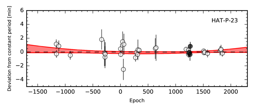
   Figure 23: Timing residuals for HAT-P-23 b. White points are data obtained and reanalyzed by Maciejewski et al. (2018) and originally reported by Bakos et al. (2011); Ramón-Fox & Sada (2013); Ciceri et al. (2015) and Sada & Ramón-Fox (2016). Black points represent new data. The red band represents the 1-$\sigma$ uncertainty in the orbital decay model.

   The best-fit orbital decay model results in $\frac{dP}{dt}=(1.47\pm 1.48)\times 10^{-10}$, consistent with a constant period. The lack of orbital decay in HAT-P-23b allows us to place a lower limit of $Q^{\prime}_{\star}>(6.4\pm 1.9)\times 10^{5}$ with 95% confidence. We refined the linear ephemeris to $t_{\rm tra}(E)=2456129.43472(09)~{}\rm{BJD_{TDB}}$ + $E\times 1.212886411(72)~{}\rm{days}$.

9. WASP-72 b was discovered by Gillon et al. (2013). It is a 1.5 $M_{\rm Jup}$ planet in a 2.2-day orbit around an F star. We have added 2 new data points to the existing collection. Because WASP-72 has a transit depth of only 0.42%, the timings have relatively low precision.

   

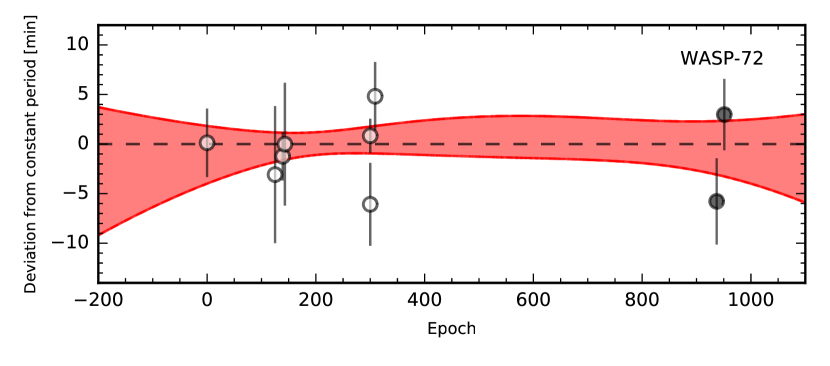
   Figure 24: Timing residuals for WASP-72 b. White points were reported by Gillon et al. (2013). Black points represent new data. The red band represents the 1-$\sigma$ uncertainty in the orbital decay model.

   The best-fit orbital decay model results in $\frac{dP}{dt}=-(5.7\pm 9.2)\times 10^{-9}$, consistent with a constant period. WASP-72 has not been observed for long enough for us to put an interesting limit on the tidal quality parameter. The available data lead to the relatively weak constraint of $Q^{\prime}_{\star}>(2.1\pm 1.4)\times 10^{3}$ with 95% confidence. We can, however, reduce the uncertainty in the orbital period by a factor of 3. The refined linear ephemeris is $t_{\rm tra}(E)=2455583.6552(11)~{}\rm{BJD_{TDB}}$ + $E\times 2.2167360(27)~{}\rm{days}$.

10. WASP-43 b, a 2 $M_{\rm Jup}$ planet in an 0.8-day orbit around a K dwarf, was discovered by Hellier et al. (2011). Since then, it has had an interesting story as far as orbital decay is concerned. Jiang et al. (2016) reported a detection of period shrinkage with $\frac{dP}{dt}=-29\pm 7$ ms yr^-1, nominally a 4-$\sigma$ detection. However, in the same year, Hoyer et al. (2016) ruled out orbital decay at that rate based on additional transit observations. Stevenson et al. (2017) added 3 transits observed with the Spitzer Space Telescope and found no evidence for orbital decay. We have significantly increased the time baseline by adding 3 new transits. In Figure 25, we compile the transit times after removing some data points based on incomplete transits. We find $\frac{dP}{dt}=(1.9\pm 0.6)\times 10^{-10}$. It appears the period of WASP-43 has increased slightly, although there are a lot of outlying data points. Whether this is just a statistical fluke will be clearer after more observations in the future. Assuming that the period is not changing, we can set a limit of $Q^{\prime}_{\star}>(2.1\pm 1.4)\times 10^{5}$ with 95% confidence. The refined linear ephemeris is $t_{\rm tra}(E)=2456342.34259(01)~{}\rm{BJD_{TDB}}$ + $E\times 0.813474059(29)~{}\rm{days}$.

    

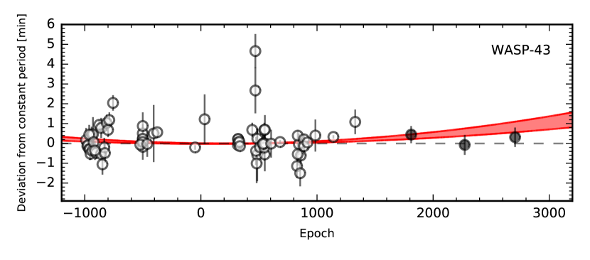
    Figure 25: Timing residuals for WASP-43 b. White points are times adopted from the literature: Gillon et al. (2012); Chen et al. (2014); Murgas et al. (2014); Stevenson et al. (2014); Ricci et al. (2015); Jiang et al. (2016); Hoyer et al. (2016); Stevenson et al. (2017). Black points show new transits and the red band represents the 1-$\sigma$ uncertainty in the orbital decay model.

11. WASP-114 b is a 1.8 $M_{\rm Jup}$ planet in 1.5-day orbit around a star somewhat hotter and more massive than the Sun. It was discovered recently, by Barros et al. (2016). The single new transit observed at FLWO is the only follow-up observation that has been reported. Since there are only two points in the timing residuals plot, it does not make much sense to fit an orbital decay model. The red band in Figure 26, therefore represents the 1-$\sigma$ uncertainty on the linear ephemeris, which we calculate to be $t_{\rm tra}(E)=2456667.73661(21)~{}\rm{BJD_{TDB}}$ + $E\times 1.548777461(81)~{}\rm{days}$.

    

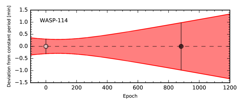
    Figure 26: Timing residuals for WASP-114 b. The white point is from Barros et al. (2016). and the black point represents new data point. The red band depicts 1$\sigma$ uncertainty on the linear ephemeris.

12. WASP-122 b is a 1.3 $M_{\rm Jup}$ planet in a 1.7-day orbit around a G star. It was discovered by Turner et al. (2016). Unfortunately, we were not able to obtain any new data, so we present it here simply to call attention to its favorable properties and its place in the “top dozen” systems to watch for orbital decay.

5 Summary

	constant period		orbital decay
Name	$t_{0}$ (BJDTDB)	$P$ (d)	$t_{0}$ (BJDTDB)	$P$ (d)	$dP/dt$	$Q_{\star}^{\prime}$
WASP-18	2458022.12523(02)	0.941452425(22)	2458022.12529(06)	0.94145230(13)	$(-1.2\pm 1.3)\times 10^{-10}$	$>\,(1.7\pm 0.4)\times 10^{6}$
KELT-16	2457910.03913(11)	0.96899319(30)	2457910.03918(15)	0.96899314(33)	$(-0.6\pm 1.4)\times 10^{-9}$	$>\,(0.9\pm 0.2)\times 10^{5}$
WASP-103	2456836.29630(07)	0.925545352(94)	2456836.29635(07)	0.92554483(25)	$(8.4\pm 4.0)\times 10^{-10}$	$>\,(1.1\pm 0.1)\times 10^{5}$
WASP-12	2456305.45556(03)	1.091419810(39)	2456305.45581(04)	1.091420087(46)	$(-9.97\pm 0.83)\times 10^{-10}$	$=\,(1.6\pm 0.2)\times 10^{5}$
HATS-18	2457089.90665(25)	0.83784309(28)	$\cdots$	$\cdots$	$\cdots$	$\cdots$
WASP-19	2456021.70390(02)	0.788839300(17)	2456021.70395(02)	0.788839420(31)	$(-2.06\pm 0.42)\times 10^{-10}$	$=\,(5.0\pm 1.5)\times 10^{5}$
OGLE-TR-56	2453936.60063(14)	1.21191123(16)	2453936.60059(14)	1.21191089(23)	$(3.34\pm 1.49)\times 10^{-10}$	$>\,(7.0\pm 2.1)\times 10^{5}$
HAT-P-23	2456129.43472(09)	1.212886411(72)	2456129.43466(11)	1.21288633(11)	$(1.47\pm 1.48)\times 10^{-10}$	$>\,(6.4\pm 1.9)\times 10^{5}$
WASP-72	2455583.6552(11)	2.2167360(27)	2455583.6542(20)	2.216742(11)	$(-5.7\pm 9.2)\times 10^{-9}$	$>\,(2.1\pm 1.4)\times 10^{3}$
WASP-43	2456342.34259(01)	0.813474059(29)	2456342.34259(01)	0.813474024(31)	$(1.9\pm 0.6)\times 10^{-10}$	$>\,(4.4\pm 0.3)\times 10^{5}$
WASP-114	2456667.73661(21)	1.548777461(81)	$\cdots$	$\cdots$	$\cdots$	$\cdots$
WASP-122	2456665.22401(21)	1.7100566(29)	$\cdots$	$\cdots$	$\cdots$	$\cdots$

Table 4: Summary of best-fit parameters and $Q_{\star}^{\prime}$. The lower limits on $Q^{\prime}_{\star}$ are based on the 95%-confidence lower limits on $dP/dt$, and the quoted uncertainties come from propagating the errors in $M_{\rm p}/M_{\star}$ and $a/R_{\star}$.

In this paper, we have drawn up a list of exoplanets that provide the best opportunities to detect orbital decay, according to a simple metric. We presented new transit times for 11 of those exoplanets. Except for the case of WASP-12, we do not see convincing evidence for a period change in any other system. There is some evidence for a decreasing period in WASP-19, but the data are sparse and there are some deviant data points, along with some indications that stellar activity is causing systematic errors in the transit times. This is nevertheless a good system to continue monitoring because of its extremely short period. The non-detections of orbital decay allows us to constrain the tidal quality factor for the star, the strongest limit being obtained for WASP-18: $Q_{\star}^{\prime}>(1.7\pm 0.4)\times 10^{6}$ with 95% confidence. Table 4 provides a summary of the best-fit parameters for all objects along with limits on $Q_{\star}^{\prime}$.

This is a unique time for studying orbital decay of exoplanets. The TESS mission is now underway. The main mission is to perform a nearly all-sky survey for new transiting planets. Christ et al. (2018) discussed the prospects for TESS in detecting orbital decay of Kepler planets, in particular, finding that there are at least a few systems that offer good prospects. In the course of the survey, TESS will also revisit almost all of the hot Jupiters that were previously discovered in wide-field surveys, including the dozen objects highlighted in this paper. This may lead to additional detections of period changes, or at the very least a helpful refinement in the transit ephemerides.

References

- Adams et al. (2011) Adams, E. R., López-Morales, M., Elliot, J. L., et al. 2011, ApJ, 741, 102
- Albrecht et al. (2012) Albrecht, S., Winn, J. N., Johnson, J. A., et al. 2012, ApJ, 757, 18
- Bakos et al. (2011) Bakos, G. Á., Hartman, J., Torres, G., et al. 2011, ApJ, 742, 116
- Barkaoui et al. (2019) Barkaoui, K., Burdanov, A., Hellier, C., et al. 2019, The Astronomical Journal, 157, 43
- Barker & Ogilvie (2010) Barker, A. J., & Ogilvie, G. I. 2010, MNRAS, 404, 1849
- Barros et al. (2016) Barros, S. C. C., Brown, D. J. A., Hébrard, G., et al. 2016, A&A, 593, A113
- Bean et al. (2013) Bean, J. L., Désert, J.-M., Seifahrt, A., et al. 2013, ApJ, 771, 108
- Bouma et al. (2019) Bouma, L. G., Winn, J. N., Baxter, C., et al. 2019, AJ, 157, 217
- Carone & Pätzold (2007) Carone, L., & Pätzold, M. 2007, Planet. Space Sci., 55, 643
- Chan et al. (2011) Chan, T., Ingemyr, M., Winn, J. N., et al. 2011, AJ, 141, 179
- Chen et al. (2014) Chen, G., van Boekel, R., Wang, H., et al. 2014, A&A, 563, A40
- Christ et al. (2018) Christ, C. N., Montet, B. T., & Fabrycky, D. C. 2018, arXiv e-prints, arXiv:1810.02826 [astro-ph.EP]
- Ciceri et al. (2015) Ciceri, S., Mancini, L., Southworth, J., et al. 2015, A&A, 577, A54
- Claret & Bloemen (2011) Claret, A., & Bloemen, S. 2011, A&A, 529, A75
- Collins et al. (2017) Collins, K. A., Kielkopf, J. F., & Stassun, K. G. 2017, AJ, 153, 78
- Copperwheat et al. (2013) Copperwheat, C. M., Wheatley, P. J., Southworth, J., et al. 2013, MNRAS, 434, 661
- Cowan et al. (2012) Cowan, N. B., Machalek, P., Croll, B., et al. 2012, ApJ, 747, 82
- Dawson & Johnson (2018) Dawson, R. I., & Johnson, J. A. 2018, ARA&A, 56, 175
- Delrez et al. (2018) Delrez, L., Madhusudhan, N., Lendl, M., et al. 2018, MNRAS, 474, 2334
- Dragomir et al. (2011) Dragomir, D., Kane, S. R., Pilyavsky, G., et al. 2011, The Astronomical Journal, 142, 115
- Eastman et al. (2013) Eastman, J., Gaudi, B. S., & Agol, E. 2013, PASP, 125, 83
- Eastman et al. (2010) Eastman, J., Siverd, R., & Gaudi, B. S. 2010, PASP, 122, 935
- Espinoza et al. (2019) Espinoza, N., Rackham, B. V., Jordán, A., et al. 2019, MNRAS, 482, 2065
- Essick & Weinberg (2015) Essick, R., & Weinberg, N. N. 2015, The Astrophysical Journal, 816, 18
- Foreman-Mackey et al. (2013) Foreman-Mackey, D., Hogg, D. W., Lang, D., & Goodman, J. 2013, PASP, 125, 306
- Gillon et al. (2011) Gillon, M., Jehin, E., Magain, P., et al. 2011, in European Physical Journal Web of Conferences, Vol. 11, European Physical Journal Web of Conferences, 06002
- Gillon et al. (2012) Gillon, M., Triaud, A. H. M. J., Fortney, J. J., et al. 2012, A&A, 542, A4
- Gillon et al. (2013) Gillon, M., Anderson, D. R., Collier-Cameron, A., et al. 2013, A&A, 552, A82
- Gillon et al. (2014) —. 2014, A&A, 562, L3
- Goldreich & Soter (1966) Goldreich, P., & Soter, S. 1966, Icarus, 5, 375
- Hansen (2010) Hansen, B. M. S. 2010, ApJ, 723, 285
- Hebb et al. (2009) Hebb, L., Collier-Cameron, A., Loeillet, B., et al. 2009, ApJ, 693, 1920
- Hebb et al. (2010) Hebb, L., Collier-Cameron, A., Triaud, A. H. M. J., et al. 2010, ApJ, 708, 224
- Hellier et al. (2011) Hellier, C., Anderson, D. R., Collier-Cameron, A., et al. 2011, ApJ, 730, L31
- Hellier et al. (2009) Hellier, C., Anderson, D. R., Collier Cameron, A., et al. 2009, Nature, 460, 1098
- Hoyer et al. (2016) Hoyer, S., Pallé, E., Dragomir, D., & Murgas, F. 2016, AJ, 151, 137
- Hut (1980) Hut, P. 1980, A&A, 92, 167
- Jackson et al. (2008) Jackson, B., Greenberg, R., & Barnes, R. 2008, ApJ, 678, 1396
- Jehin et al. (2011) Jehin, E., Gillon, M., Queloz, D., et al. 2011, The Messenger, 145, 2
- Jiang et al. (2016) Jiang, I.-G., Lai, C.-Y., Savushkin, A., et al. 2016, AJ, 151, 17
- Kreidberg et al. (2015) Kreidberg, L., Line, M. R., Bean, J. L., et al. 2015, ApJ, 814, 66
- Lendl et al. (2017) Lendl, M., Cubillos, P. E., Hagelberg, J., et al. 2017, A&A, 606, A18
- Lendl et al. (2013) Lendl, M., Gillon, M., Queloz, D., et al. 2013, A&A, 552, A2
- Levrard et al. (2009) Levrard, B., Winisdoerffer, C., & Chabrier, G. 2009, ApJ, 692, L9
- Maciejewski et al. (2013) Maciejewski, G., Dimitrov, D., Seeliger, M., et al. 2013, A&A, 551, A108
- Maciejewski et al. (2016) Maciejewski, G., Dimitrov, D., Fernández, M., et al. 2016, A&A, 588, L6
- Maciejewski et al. (2018) Maciejewski, G., Fernández, M., Aceituno, F., et al. 2018, Acta Astron., 68, 371
- Mancini et al. (2013) Mancini, L., Ciceri, S., Chen, G., et al. 2013, MNRAS, 436, 2
- Mandel & Agol (2002) Mandel, K., & Agol, E. 2002, ApJ, 580, L171
- Matsakos & Königl (2015) Matsakos, T., & Königl, A. 2015, ApJ, 809, L20
- Maxted et al. (2013) Maxted, P. F. L., Anderson, D. R., Doyle, A. P., et al. 2013, MNRAS, 428, 2645
- Mayor & Queloz (1995) Mayor, M., & Queloz, D. 1995, Nature, 378, 355
- McDonald & Kerins (2018) McDonald, I., & Kerins, E. 2018, MNRAS, 477, L21
- Mortier et al. (2013) Mortier, A., Santos, N. C., Sousa, S. G., et al. 2013, A&A, 558, A106
- Murgas et al. (2014) Murgas, F., Pallé, E., Zapatero Osorio, M. R., et al. 2014, A&A, 563, A41
- Narita et al. (2015) Narita, N., Fukui, A., Kusakabe, N., et al. 2015, Journal of Astronomical Telescopes, Instruments, and Systems, 1, 045001
- Oberst et al. (2017) Oberst, T. E., Rodriguez, J. E., Colón, K. D., et al. 2017, AJ, 153, 97
- Ogilvie (2014) Ogilvie, G. I. 2014, ARA&A, 52, 171
- Patra et al. (2017) Patra, K. C., Winn, J. N., Holman, M. J., et al. 2017, AJ, 154, 4
- Penev et al. (2018) Penev, K., Bouma, L. G., Winn, J. N., & Hartman, J. D. 2018, AJ, 155, 165
- Penev et al. (2012) Penev, K., Jackson, B., Spada, F., & Thom, N. 2012, ApJ, 751, 96
- Penev et al. (2016) Penev, K., Hartman, J. D., Bakos, G. Á., et al. 2016, AJ, 152, 127
- Pojmanski (1997) Pojmanski, G. 1997, Acta Astron., 47, 467
- Pont et al. (2007) Pont, F., Moutou, C., Gillon, M., et al. 2007, A&A, 465, 1069
- Ramón-Fox & Sada (2013) Ramón-Fox, F. G., & Sada, P. V. 2013, Rev. Mexicana Astron. Astrofis., 49, 71
- Rasio et al. (1996) Rasio, F. A., Tout, C. A., Lubow, S. H., & Livio, M. 1996, ApJ, 470, 1187
- Ricci et al. (2015) Ricci, D., Ramón-Fox, F. G., Ayala-Loera, C., et al. 2015, PASP, 127, 143
- Ricker et al. (2015) Ricker, G. R., Winn, J. N., Vanderspek, R., et al. 2015, Journal of Astronomical Telescopes, Instruments, and Systems, 1, 014003
- Sada & Ramón-Fox (2016) Sada, P. V., & Ramón-Fox, F. G. 2016, PASP, 128, 024402
- Sada et al. (2012) Sada, P. V., Deming, D., Jennings, D. E., et al. 2012, PASP, 124, 212
- Sasselov (2003) Sasselov, D. D. 2003, ApJ, 596, 1327
- Schlaufman & Winn (2013) Schlaufman, K. C., & Winn, J. N. 2013, ApJ, 772, 143
- Shporer et al. (2019) Shporer, A., Wong, I., Huang, C. X., et al. 2019, AJ, 157, 178
- Southworth et al. (2015) Southworth, J., Mancini, L., Ciceri, S., et al. 2015, MNRAS, 447, 711
- Stassun et al. (2017) Stassun, K. G., Collins, K. A., & Gaudi, B. S. 2017, AJ, 153, 136
- Stevenson et al. (2014) Stevenson, K. B., Bean, J. L., Seifahrt, A., et al. 2014, AJ, 147, 161
- Stevenson et al. (2017) Stevenson, K. B., Line, M. R., Bean, J. L., et al. 2017, AJ, 153, 68
- Teitler & Königl (2014) Teitler, S., & Königl, A. 2014, ApJ, 786, 139
- Torres et al. (2012) Torres, G., Fischer, D. A., Sozzetti, A., et al. 2012, ApJ, 757, 161
- Torres et al. (2004) Torres, G., Konacki, M., Sasselov, D. D., & Jha, S. 2004, The Astrophysical Journal, 609, 1071
- Torres et al. (2008) Torres, G., Winn, J. N., & Holman, M. J. 2008, The Astrophysical Journal, 677, 1324
- Tregloan-Reed et al. (2013) Tregloan-Reed, J., Southworth, J., & Tappert, C. 2013, MNRAS, 428, 3671
- Turner et al. (2017) Turner, J. D., Leiter, R. M., Biddle, L. I., et al. 2017, MNRAS, 472, 3871
- Turner et al. (2016) Turner, O. D., Anderson, D. R., Collier Cameron, A., et al. 2016, PASP, 128, 064401
- Villaver & Livio (2009) Villaver, E., & Livio, M. 2009, ApJ, 705, L81
- Weinberg et al. (2017) Weinberg, N. N., Sun, M., Arras, P., & Essick, R. 2017, ApJ, 849, L11
- Wilkins et al. (2017) Wilkins, A. N., Delrez, L., Barker, A. J., et al. 2017, ApJ, 836, L24
- Winn (2010) Winn, J. N. 2010, Exoplanet Transits and Occultations, ed. S. Seager (University of Arizona Press), 55
- Yee et al. (2020) Yee, S. W., Winn, J. N., Knutson, H. A., et al. 2020, ApJ, 888, L5