Monitoring strong coupling in nonlocal plasmonics with electron spectroscopies

Abstract

Plasmon–exciton polaritons provide exciting possibilities to control light–matter interactions at the nanoscale by enabling closer investigation of quantum optical effects and facilitating novel technologies based, for instance, on Bose–Einstein condensation and polaritonic lasing. Nevertheless, observing and visualising polaritons is challenging, and traditional optical microscopy techniques often lead to ambiguities regarding the emergence and strength of the plasmon–exciton coupling. Electron microscopy offers a more robust means to study and verify the nature of plexcitons, but is still hindered by instrument limitations and resolution. A simple theoretical description of electron beam-excited plexcitons is therefore vital to complement ongoing experimental efforts. Here we apply analytic solutions for the electron-loss and photon-emission probabilities to evaluate plasmon–exciton coupling studied either with the recently adopted technique of electron energy-loss spectroscopy, or with the so-far unexplored in this context cathodoluminescence spectroscopy. Foreseeing the necessity to account for quantum corrections in the plasmonic response, we extend these solutions within the framework of general nonlocal hydrodynamic descriptions. As a specific example we study core–shell spherical emitter–molecule hybrids, going beyond the standard local-response approximation through the hydrodynamic Drude model for screening and the generalised nonlocal optical response theory for nonlocal damping. We show that electron microscopies are extremely powerful in describing the interaction of emitters with the otherwise weakly excited by optical means higher-order plasmonic multipoles, a response that survives when quantum-informed models are considered. Our work provides therefore both a robust theoretical background and supporting argumentation to the open quest for improving and further utilising electron microscopies in strong-coupling nanophotonics.

I Introduction

Electron-beam spectroscopies have been rapidly gaining their well-deserved share of attention in nanophotonics, as they have opened new pathways for the optical characterisation of state-of-the-art nanoscale architectures Polman et al. (2019). Electron energy-loss spectroscopy (EELS) has proven time and again efficient in mapping the localised surface plasmon (LSP) modes of metallic nanoparticles (NPs), thus offering unique insight into nanoscopic optical processes Nelayah et al. (2007); Bosman et al. (2007), including the possibilities to optically excite dark modes in NPs Koh et al. (2009), or map plasmons in novel materials such as graphene Eberlein et al. (2008); Zhou et al. (2012). Of particular importance in this context is the realisation that EELS can be a more accurate probe for nanoscale effects of quantum origin Scholl et al. (2012); Raza et al. (2013), thus accelerating the growth of quantum plasmonics Tame et al. (2013); Zhu et al. (2016); Bozhevolnyi and Mortensen (2017); Fernández-Domínguez et al. (2018). Complementary to the near-field-oriented EELS is cathodoluminescence (CL) spectroscopy, which is more efficient at probing radiative modes excited by subnanometre electron beams Vesseur et al. (2007); Gómez-Medina et al. (2008); Losquin et al. (2015). Combining these two techniques, a richness of information on the response of nanophotonic architectures can be acquired Kuttge et al. (2009); Chaturvedi et al. (2009); Yamamoto et al. (2011); Raza et al. (2015a).

Recently, EELS was theoretically proposed Konečná et al. (2018), Crai et al. (2019) and experimentally explored Yankovich et al. (2019), Bitton et al. (2020) as an alternative technique for monitoring strong coupling in nanophotonics and visualising the formation of hybrid exciton-polaritons. In particular, EELS was experimentally used to trace the anticrossing of two hybrid modes in truncated nanopyramids coupled to excitons in transition-metal dichalcogenides Yankovich et al. (2019), and in quantum dots coupled to dark bowtie-antenna modes Bitton et al. (2020), illustrating how electron spectroscopies have nothing to envy from their optical counterparts, but can in fact be more efficient when dark modes are involved. Inspired by quantum optics, strong coupling is among the most rapidly growing areas in photonics Törmä and Barnes (2015); Baranov et al. (2018), because it combines the possibility to assess quantum-optical concepts without the need for extreme laboratory conditions Yoshie et al. (2004); Dovzhenko et al. (2018); Ojambati et al. (2019); Tserkezis et al. (2019) with the promise of technological advances in a diversity of areas such as optical nonlinearities Sanvitto and Kéna-Cohen (2016), logic gates and circuits Liew et al. (2008), polariton lasing Kéna-Cohen and Forrest (2010), Bose–Einstein condensation Hakala et al. (2018), or via modification of the properties of matter through polaritonic chemistry Feist et al. (2018) and enablement of forbidden transitions Cuartero-González and Fernández-Domínguez (2018). For this reason, a plethora of designs has been proposed, ranging from planar metallic films Pockrand et al. (1982); Bellessa et al. (2004) and metallic NP arrangements Zengin et al. (2015); Chikkaraddy et al. (2016); Todisco et al. (2016); Chatzidakis and Yannopapas (2019) combined with organic molecules, to quantum dots Santhosh et al. (2016) or two-dimensional materials Liu et al. (2016); Geisler et al. (2019) in nanophotonic cavities. Most of these designs exploit the tremendous field confinement provided by plasmonics, although dielectric nanocavities with lower losses are now emerging as attractive alternatives Wang et al. (2016); Lepeshov et al. (2018); Tserkezis et al. (2018a); Todisco et al. (2019). Nevertheless, despite their different approaches in terms of design and application, what the vast majority of these works have in common is the use of optical microscopy as the key analysis technique.

Here we turn to more recent efforts to introduce electron microscopy as a tool for exploring strong coupling Konečná et al. (2018); Crai et al. (2019); Yankovich et al. (2019); Bitton et al. (2020), and take them one step further by showing that both EELS and CL can provide information about the occurrence of hybridisation. Furthermore, anticipating the fabrication of architectures with even finer geometrical details, we develop the appropriate framework to include quantum effects in the plasmonic response on the basis of standard or more generalised hydrodynamic models Kosionis et al. (2012); Christensen et al. (2014); Raza et al. (2015b); Tserkezis et al. (2018b), appropriately extending very recent theoretical descriptions of classical strong coupling Crai et al. (2019). While the composites studied here are relatively unrealistic with modern technology, and somehow simplified in terms of design, they can be described by exact analytic solutions which can be used for benchmarking any computational schemes designed to describe more realistic examples. Focusing on core–shell NPs, we provide analytic solutions for the electron energy-loss (EEL) and photon-emission (PE) probabilities, which are valuable, not only for obtaining a clear physical interpretation, but also for benchmarking more elaborate designs. As an illustrative example, we show that the spectral anticrossing anticipated for Ag nanospheres covered by, or encapsulating an excitonic layer, can be efficiently traced in EEL and PE probabilities. Such tools can be advantageous when the excitons couple to the dominant dipolar plasmon mode, but even more so in the case of higher-order multipoles, whose linewidths might be better comparable to those of the excitons, but whose prevailing non-radiative nature makes their exploration with optical microscopies problematic. Recent experiments Raza et al. (2015a) have shown that higher-order multipole modes indeed contribute to the EELS signal of ultrasmall nanospheres, with sensitivity that goes way beyond the capabilities of optical spectroscopies. We thus believe that our work will provide additional motivation to further invest in exploring strong coupling with electron microscopy.

II Analytic solutions

Let us first describe the general framework for investigating plasmon–exciton coupling in the local-response approximation (LRA) in the case of spherical NPs. Typically, the LRA regime corresponds to NP radii larger than $\sim 20$ nm, for which nonlocal effects are not relevant Tserkezis et al. (2018a). The plexcitonic configuration employed here is based on the core–shell geometry, with either a plasmonic sphere of radius $R_{1}$ covered by an excitonic shell of outer radius $R_{2}$, as shown in Fig. 1(a), or a plasmonic shell (outer radius $R_{2}$) encapsulating an excitonic core (radius $R_{1}$), as shown in Fig. 1(c). In either case, the excitation is a swift electron of velocity $\nu$ travelling at a distance $d$ — the impact parameter — from the NP centre (taken as the coordinate origin). In our calculations we set $d=70$ nm and $\nu=0.69\;c$, $c$ being the velocity of light in vacuum. Neglecting relativistic effects, the latter corresponds to a kinetic energy of $\sim$120 keV. The relative permittivity $\varepsilon_{\mathrm{m}}$ of the plasmonic component as a function of angular frequency $\omega$ follows a Drude model Bohren and Huffman (1983), i.e., $\varepsilon_{\mathrm{m}}(\omega)=\varepsilon_{\infty}(\omega)-\omega_{\mathrm{p}}^{2}/[\omega(\omega-\mathrm{i}\gamma_{\mathrm{m}})]$ (throughout this paper we assume an $\exp(\mathrm{i}\omega t)$ time dependence of the fields), where $\varepsilon_{\infty}$ accounts for interband transitions, $\omega_{\mathrm{p}}$ is the plasma frequency, and $\gamma_{\mathrm{m}}$ is the damping rate in the metal. In this study we employ Ag, described by $\varepsilon_{\infty}=5$ Yang et al. (2015), $\hbar\omega_{\mathrm{p}}=8.99$ eV, and $\hbar\gamma_{\mathrm{m}}=0.025$ eV Raza et al. (2015b). These values provide a good Drude fit of the experimental data by Johnson and Christy Johnson and Christy (1972) in the free-electron regime, while for $\varepsilon_{\infty}$ we use the value given in Ref. Yang et al. (2015), to keep it constant for simplicity. The relative permittivity $\varepsilon_{\mathrm{e}}$ of the excitonic material is modeled by a Drude–Lorentz model as $\varepsilon_{\mathrm{e}}(\omega)=1-f\omega_{\mathrm{e}}^{2}/[\omega(\omega-\mathrm{i}\gamma_{\mathrm{x}})-\omega_{\mathrm{e}}^{2}]$, with $\hbar\omega_{\mathrm{e}}=2.7$ eV, $\hbar\gamma_{\mathrm{x}}=0.052$ eV, and reduced oscillator strength $f=0.02$ Fofang et al. (2008); Tserkezis et al. (2018b).

To calculate the EEL and PE probabilities, we expand the incident electric field due to a moving electron, and also the scattered field and the fields inside the NP, into vector spherical waves García de Abajo (1999, 2010) and apply the boundary conditions of continuity of the tangential components of the fields at the interfaces between two different media to obtain the scattering matrix that associates the amplitude of the scattered field to the incident field. With this approach the PE and the EEL probabilities can be derived as García de Abajo (1999); Matyssek et al. (2012a)

$$P_{\mathrm{PE}}=\frac{c^{3}}{4\pi^{2}\omega^{3}}\sum_{\stackrel{{\scriptstyle m=-\infty}}{{l=|m|}}}^{\infty}l\left(l+1\right)\left(\left|F_{lm}\right|^{2}+\left|G_{lm}\right|^{2}\right),$$ (1)

$$P_{\mathrm{EEL}}=\frac{1}{\pi\omega^{2}}\sum_{\stackrel{{\scriptstyle m=-\infty}}{{l=|m|}}}^{\infty}\left\{m\nu K_{m}\left(\frac{\omega d}{\nu\gamma}\right)\mathrm{Re}\left[(A_{lm}^{+})^{\ast}\mathrm{i}F_{lm}\right]+\frac{c}{2\gamma}K_{m}\left(\frac{\omega d}{\nu\gamma}\right)\mathrm{Re}\left[(B_{lm}^{+})^{\ast}\mathrm{i}G_{lm}\right]\right\}~{},$$ (2)

where ${\mathrm{Re}}[\cdot]$ represents the real part of the function in square brackets, and the star denotes complex conjugation. In these expressions $l$ and $m$ are the standard angular momentum indices, $\gamma=1/\sqrt{1-\nu^{2}/c^{2}}$, $K_{m}$ is the modified Bessel function, and $A_{lm}^{+}$, $B_{lm}^{+}$, $F_{lm}$ and $G_{lm}$ are appropriate expansion coefficients (see Appendix).

When at least one of the characteristic dimensions of the system (i.e., $R_{1}$, $R_{2}$, $R_{2}-R_{1}$, or $d$) becomes comparable to the mean free-electron path, quantum-informed models for the description of the plasmonic NP response become relevant Zhu et al. (2016); Tserkezis et al. (2018c). Traditional or more advanced hydrodynamic models are among the most appealing approaches, because they immediately account for the longer-scale effect of screening, and various implementations in numerical tools based on boundary elements Trügler et al. (2017), finite elements Toscano et al. (2012), finite differences in time domain McMahon et al. (2010), or discrete sources Eremin et al. (2018), have been developed to tackle NPs of arbitrary shapes, while schemes that can include electron spill-out have also appeared Toscano et al. (2015); Ciracì and Della Sala (2016). Electron spill-out and tunneling become relevant at even shorter lengths scales Yan et al. (2015), and require hybrid models that take as input fully quantum-mechanical calculations Esteban et al. (2012); Hohenester (2015); Yannopapas (2017); Ciracì et al. (2019). Since, however, we are interested in exactly solvable analytic solutions, we will resort here to the standard hydrodynamic Drude model (HDM) Ruppin (1973) that accounts for screening, and the generalised nonlocal optical response (GNOR) theory Mortensen et al. (2014) for nonlocal damping. To take nonlocal effects in the metal into account with these approaches, a longitudinal term needs to be included in the expansion of the field, and we employ the standard additional boundary condition of continuity of the normal component of the displacement field for the no spill-out case (hard-wall boundary conditions) Tserkezis et al. (2016), which, despite its simplicity, provides an adequate description of noble metals like Ag Teperik et al. (2013).

III Plasmon–exciton coupling in LRA

In Fig. 1(b) we show EEL spectra (blue curve) for an Ag sphere in air (as shown in the left-hand schematics of Fig. 1(a)). Its radius, $R_{1}$, is set equal to $60$ nm so that its dipolar LSP resonance coincides with the $2.7$ eV resonance energy of the excitonic material. The dipolar LSP resonance of the Ag sphere manifests in the EEL spectra as a broad peak at $2.7$ eV. A smaller NP radius would blueshift the dipolar LSP (e.g. to $3.14$ eV for $R_{1}=40$ nm), leading to detuning with $\hbar\omega_{\mathrm{e}}$. Accordingly, larger radii redshift the LSP modes, thus allowing to fully tune the response. Adding, next, a $5$ nm-thick excitonic shell (so that $R_{2}=65$ nm), as shown in the right-hand schematics of Fig. 1(a), has as an immediate consequence the interaction of the excitonic mode with the dipolar LSP. Two coupled hybrid modes thus emerge, and their characteristic anticrossing appears in the spectra, and in standard resonance energy vs detuning diagrams (not shown here). The spectra of the coupled system are plotted with the red curve in Fig. 1(b). Clearly, due to the small oscillator strength and the thinness of the excitonic shell, the two hybrid modes are not well-discernible; while the first hybrid resonance is well localised at $2.71$ eV, the second one, around $2.86$ nm, is less intense and not well localised, but almost damped (see inset of Fig. 1(b)). This is a typical case of weak plasmon–exciton coupling. An attempt to match the higher-order multipoles of the Ag sphere (appearing in the EEL spectra at around $3.5$ eV) to $\hbar\omega_{\mathrm{e}}$ by further increasing $R_{1}$, results in damped and broadened resonances. Consequently, the Ag core–exciton shell geometry proves inefficient in the attempt to achieve a clear Rabi-like splitting for the dipolar LSP, let alone for higher-order modes, which our intention is to explore here.

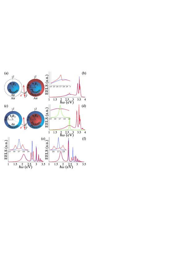
Figure 1: (a) Schematics of the Ag core–exciton shell set-up. (b) EEL spectra for the set-up of (a), taking $R_{1}=60$ nm and $R_{2}=65$ nm. Blue curves correspond to the bare Ag NP spectra [left-hand schematic in (a)], while red curves correspond to the full core–shell NP [right-hand schematic in (a)]. (c) Schematics of the exciton core–Ag shell set-up. (d)–(f) EEL spectra for the set-up of (c), for three different combinations of radii, so as to align the dipolar, quadrupolar, and octapolar LSP of the Ag shell to the exciton energy. In (d) $R_{1}=33$ nm and $R_{2}=60$ nm, leading to two hybrid resonances separated by a shallow dip, with separation of $\hbar\Omega=0.1$ eV. In (e) $R_{1}=51.2$ nm and $R_{2}=60$ nm. The anticrossing between the quadrupolar Ag shell LSP and the exciton is $0.16$ eV. Finally, in (f) $R_{1}=54.2$ nm and $R_{2}=60$ nm, and the anticrossing between the octapolar LSP of the shell and the exciton is $0.18$ eV. In all calculations, the impact parameter is $d=70$ nm, while the electron speed is $\nu=0.69\;c$. The green curve in (d) corresponds to the bare excitonic NP spectra [left-hand schematic in (a) where now the core is excitonic instead of plasmonic]. All insets are zooms in the energy regions of the relevant resonances.

The plasmonic–excitonic configuration of Fig. 1(c) is more promising for observing the splitting, not only for the dipolar, but also for the quadrupolar and the octapolar LSP resonances. Such a nanostructure may be more challenging to fabricate, but on the other hand protects the excitonic material (especially in case of organic molecules) from the intense exciting electron beam. Initially, the thickness $R_{2}-R_{1}$ of the plasmonic shell, in the absence of the core (left-hand schematic of Fig. 1(c)) is engineered such that each resonance is tuned to the transition energy of the excitonic material. Then, by introducing the excitonic core (right-hand schematic of Fig. 1(c)), plasmon–exciton coupling is allowed to take place. This is illustrated in Figs 1(d)–(f) for the dipolar, quadrupolar and octapolar LSP resonance, respectively. The blue curves in each figure are the EEL spectra in the absence of the excitonic core, showing that indeed the mode is tuned to $2.7$ eV. The red curves illustrate the splitting in each case, while the insets zoom in the corresponding spectral window of interest. This set-up reveals that a clear Rabi-like splitting can be achieved for both higher-order modes, whilst the dipolar LSP interacts only weakly with the exciton. This weak interaction, typical of what has been termed induced transparency region Zengin et al. (2013), could be anticipated by observing separately the linewidths of the dipolar LSP (Ag shell in the absence of the excitonic core) and the excitonic resonance (excitonic core in the absence of a shell). The EEL spectrum of this latter mode is depicted with the green curve in Fig. 1(d). The linewidth of the excitonic mode is estimated equal to $0.0298$ eV, much narrower than the broad linewidth of the LSP. To verify that the system has indeed entered the strong coupling regime in the case of the higher-order LSP modes of Figs 1(e) and (f), we check whether the observed energy splittings $\hbar\Omega$ satisfy the strong coupling condition involving the plasmonic ($\gamma_{\mathrm{p}}$) and excitonic ($\gamma_{\mathrm{e}}$) resonance linewidths Törmä and Barnes (2015)

$$\hbar\Omega>\left[\frac{(\hbar\gamma_{\mathrm{p}})^{2}}{2}+\frac{(\hbar\gamma_{\mathrm{e}})^{2}}{2}\right]^{1/2}~{}.$$ (3)

In principle, there is also an additional contribution to the broadening from the interaction with the electron beam, $\gamma_{\mathrm{p-e}}$. Since we are not strictly interested in displaying a particular strong-coupling architecture, we will disregard this in what folllows, assuming that $\gamma_{\mathrm{p-e}}\ll\gamma_{\mathrm{p,rad}}$, where $\gamma_{\mathrm{p,rad}}$ is the radiation contribution to $\gamma_{\mathrm{p}}$. Through Lorentzian fittings for the quadrupolar and octapolar LSPs in the absence of the excitonic core and in the absence of the Ag shell, we obtain $\hbar\gamma_{\rm p}=0.0196$ eV and $\hbar\gamma_{\rm e}=0.03$ eV for the case of the quadrupolar mode, and $\hbar\gamma_{\rm p}=0.0177$ eV and $\hbar\gamma_{\rm e}=0.03$ eV for the case of the octapolar mode. These calculations yield $0.0253$ eV and $0.0246$ eV for the quadrupolar and octapolar mode, respectively, as computed by the right-hand side of Eq. (3). On the other hand, the difference between the two hybrid resonances in Fig. 1(e) and (f) is $\hbar\Omega=0.16$ eV and $\hbar\Omega=0.18$ eV, for the quadrupolar and the octapolar mode respectively, values always greater that the aforementioned calculated ones from the right-hand side of Eq. (3). Thus we deduce a distinguishable lower- and higher-order multipolar strong plasmon–exciton coupling in EELS.

IV Higher-order plexcitons within quantum-informed models

Having established that higher-order multipole LSP modes can efficiently couple with excitons, we go one step further to evaluate how this coupling is affected by the triggering of quantum effects, relevant for small NP dimensions (typically below $5$ nm in radius), utilising HDM and GNOR as our quantum-informed models. At this scale, nonlocality plays a decisive role in determining the spectral features Tserkezis et al. (2016), and it is taken into account by introducing a compressible electron fluid characterised by a Fermi velocity $v_{\mathrm{F}}=1.39\times 10^{6}$   m/s and a diffusion constant $D=3.61\times 10^{-4}$   m²/s to mimic surface-enhanced Landau damping, values suitable for Ag Raza et al. (2015b) (see also Appendix). Since the configuration of Fig. 1(a) does not reveal clear anticrossings, we restrict ourselves to the set-up of Fig. 1(c).

We begin our investigation with HDM. The blue dashed and solid curves in Fig. 2(a) depict EEL spectra for LRA and HDM, respectively, in the absence of the excitonic core (hollow Ag shell). In this example the impact parameter is set at $d=5$ nm. The electron velocity is kept at $\nu=0.69\;c$, the outer radius is $R_{2}=4$ nm, and a shell thickness of $0.9$ nm (implying that $R_{1}=3.1$ nm) is such that the LSP dipolar mode of the air–Ag set-up, as calculated within HDM, matches the transition energy of the excitonic material ($2.7$ eV). This is shown by the blue solid curve in Fig. 2(a). With the same thickness, the LRA dipolar LSP is located at $2.68$ eV. In these spectra one can also observe the higher-order (quadrupolar) LRA mode at $3.08$ eV, and the corresponding HDM quadrupolar LSP at $3.15$ eV. Both dipolar and quadrupolar HDM modes exhibit the anticipated blueshifts as compared to their LRA counterparts Christensen et al. (2014). When the dye is introduced, plasmon–exciton coupling takes place with the same $\hbar\Omega=0.15$ eV for both LRA and HDM, as illustrated by the red dashed and solid curves in the inset of Fig. 2(a). Evidently, nonlocality does not affect the width of the anticrossing, but rather shifts both hybrid modes by the same amount Tserkezis et al. (2018b), as one can observe in the inset of Fig. 2(a). Interestingly, unlike Fig. 1, here strong coupling with the dipolar LSP mode can be achieved, as the dimensions of the dye layer are such that the excitonic resonance is comparable in strength. Indeed, the uncoupled plasmonic and excitonic modes exhibit narrow linewidths ($\hbar\gamma_{\rm p}=0.0119$ eV, $\hbar\gamma_{\rm e}=0.0247$ eV, as calculated within HDM). These values yield a collective linewidth (what enters the right-hand side of Eq. (3)) of $0.019$ eV, much less than the observed $\hbar\Omega=0.15$ eV, thus satisfying the strong coupling condition of Eq. (3). In Fig. 2(b) we re-engineer the hollow Ag shell so that now the HDM quadrupolar LSP is tuned to $2.7$ eV (blue solid curve), by setting a $0.49$ nm thickness, while keeping $R_{2}=4$ nm. With this thickness, the LRA quadrupolar LSP appears at $2.65$ eV (blue dashed curve in the inset of Fig. 2(b), with $\hbar\gamma_{\rm p}=0.0103$ eV). Introducing the excitonic core ($\hbar\gamma_{\rm e}=0.0247$ eV), higher-order Rabi-like splitting is observed, as shown in Fig. 2(b) by the red curves, with $\hbar\Omega=0.17$ eV. Furthermore, we note that the slight increase of the radius of the shell, from $3.1$ nm to $3.51$ nm does not affect the exciton linewidth. Ultimately, the blueshift behaviour due to HDM is inherited by the higher-order hybrid modes. In Figs 2(c) and (d) we repeat the study of Figs 2(a) and (b), respectively, by increasing the $\hbar\gamma_{\rm m}$ value used in Drude model from $0.025$ eV Raza et al. (2015b) to $0.039$ eV Yang et al. (2015), to see how an increased classical damping that might be experimentally relevant, affects the spectra. As it is evident, the system still enters the strong coupling regime, with $\hbar\Omega=0.146$ eV, $\hbar\gamma_{\rm p}=0.0415$ eV, and $\hbar\gamma_{\rm e}=0.0247$ eV for the dipolar HDM mode [Fig. 2(c)], and $\hbar\gamma_{\rm p}=0.0379$ eV, $\hbar\gamma_{\rm e}=0.0247$ eV, $\hbar\Omega=0.169$ eV for the quadrupolar modes of Fig. 2(d).

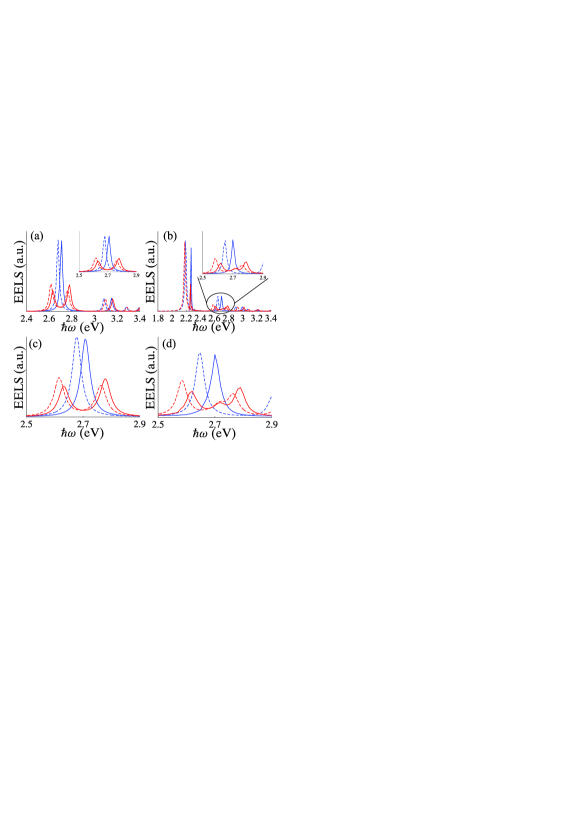
Figure 2: Dipolar and quadrupolar higher-order Rabi-like splitting in plexcitonics as predicted by HDM. In all calculations, the impact parameter is $d=5$ nm and the electron velocity is $\nu=0.69\;c$. (a) Plasmon–exciton coupling for the dipolar LSP mode, when $R_{1}=3.1$ nm and $R_{2}=4$ nm. The blue dashed curve depicts the EEL spectrum for the set-up of the left-hand schematic of Fig. 1(c) within LRA, while the blue solid curve shows the corresponding spectrum within HDM. Red curves correspond to the presence of the excitonic core, as in the right-hand schematic of Fig. 1(c). The inset zooms in the energy window of interest. (b) Quadrupolar LSP–exciton coupling for $R_{1}=3.51$ nm and $R_{2}=4$ nm. The blue/red dashed curves depict the EEL spectrum within LRA without/with the excitonic core and the blue/red solid curves are the EEL spectrum within HDM without/with the excitonic core present. (c) EEL spectrum as in the inset of (a). All the values of parameters are the same as in (a) except for $\hbar\gamma_{\rm m}=0.039$ eV in Drude model for Ag. (d) EEL spectrum as in the inset of (b). All the values of parameters are the same as in (b) except for $\hbar\gamma_{\rm m}=0.039$ eV in Drude model for Ag.

In Fig. 3 we take our nonlocal treatment one step further, to apply the GNOR theory, which is expected to lead to significant mode broadening due to surface-enhanced Landau damping Tserkezis et al. (2018c). To directly compare with Fig. 2, we maintain the same impact parameter, electron velocity, and outer NP radius, and only change $R_{1}$ to tune the plasmonic response. The blue dashed and solid curves in Fig. 3(a) depict EEL spectra for LRA and GNOR, respectively, in the presence of a hollow core. In this case we set $R_{1}=3.1$ nm so that the GNOR LSP dipolar mode of the hollow Ag set-up is tuned to $2.7$ eV, while the quadrupolar LSP is located at $3.16$ eV. Both GNOR modes exhibit the anticipated blueshifts, and in addition, nonlocal damping and broadening Christensen et al. (2014). Nevertheless, this additional surface-enhanced Landau damping does not prevent the system from entering the strong coupling regime, once the excitonic core is introduced, with $\hbar\Omega=0.15$ eV (for both LRA and GNOR models) as illustrated by the red dashed and solid curves in the inset of Fig. 3(a), since the linewidths of the uncoupled modes are $\hbar\gamma_{\rm p}=0.0277$ eV and $\hbar\gamma_{\rm e}=0.0247$ eV.

Since we are more interested in higher-order multipoles, in Fig. 3(b) the hollow Ag shell is designed to bring the GNOR quadrupolar LSP at $2.7$ eV (see inset), by setting a $R_{1}=3.51$ nm. Introducing the excitonic core, strong coupling with the quadrupolar LSP is observed, as shown in Fig. 3(c), with $\hbar\Omega=0.18$ eV. The corresponding uncoupled mode linewidths are $\hbar\gamma_{\rm p}=0.0483$ eV and $\hbar\gamma_{\rm e}=0.0247$ eV, thus fully satisfying Eq. (3). Nevertheless, in this case, in addition to the two hybrid exciton-polaritons, an intermediate resonance is present at $2.72$ eV (see also inset of Fig. 3(c)). To conclude about the nature of this mode, we resort to the LRA spectrum (red dashed curve in this inset). As it is evident, the two emerged hybrid modes are subject to blueshifts and broadening due to nonlocality in the metal. Nevertheless, the middle resonance is unaffected by nonlocality, implying that it corresponds to a surface exciton polariton (SEP) mode Gentile and Barnes (2017). This mode, attributed to the geometrical resonance of a spherical shell with a negative permeability Antosiewicz et al. (2014), was recently found to be involved in the dipolar Rabi-like splitting of a dielectric–plasmonic–excitonic set-up Tserkezis et al. (2018b). Here it is observed that it can also exist during higher-order plasmon–exciton coupling in electron probed systems. Fig. 3(d) depicts the spatial localisation of the two coupled hybrid modes and the SEP, on the outer surface of the molecule. These maps show that, by setting the energy of the swift electron to the respective value of the resonance, the localised electric field pattern is revealed, even at the close neighborhood of the source. Of course, in modern electron microscopes this tuneability is not available (they typically operate at a couple of high voltages), stressing thus the importance of flexibility provided by the core–shell geometry. Additionally, all three modes have the same spatial distribution around the surface of the outer sphere, also observed in electron probed nanorods Konečná et al. (2018) and nanopyramids Yankovich et al. (2019).

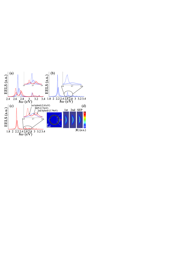
Figure 3: Dipolar and higher-order Rabi-like splitting in plexcitonics as obtained within GNOR. In all calculations, the impact parameter $d$ and the electron velocity $\nu$ are the same with those in Fig. 2. (a) Plasmon–exciton coupling for the dipolar LSP mode, when $R_{1}=3.1$ nm and $R_{2}=4$ nm. The blue dashed curve depicts the EEL spectrum for the set-up of the left-hand schematic of Fig. 1(c) within LRA, while the blue solid curve shows the corresponding spectrum within GNOR. Red curves correspond to the presence of the excitonic core. The inset zooms in the energy window of interest. (b) The quadrupolar LSP resonances (in the absence of the excitonic core) for $R_{1}=3.51$ nm and $R_{2}=4$ nm. The blue dashed curve is the EEL spectrum obtained within LRA, while the solid curve is the corresponding result within GNOR. (c) Red curves are the corresponding to (b) EEL spectra when the excitonic core is present. The blue solid curve in the inset of (c) is as in (b). (d) Near-field plots for the two coupled hybrid modes and for the SEP mode shown in the inset of (c). The red bullet depicts the location of the moving electron.

Apart from EELS, CL spectroscopy is also attracting more and more attention in nanophotonics van Wijngaarden et al. (2006); Chaturvedi et al. (2009); Gómez-Medina et al. (2008); Jeannin et al. (2017). To establish CL as an equally powerful tool for the study of strong coupling and quantum plasmonics at the same time, at least when radiative modes are involved, we proceed to calculate PE probabilities within both classical and hydrodynamic frameworks. In Fig. 4(a) we plot PE spectra for the same core–shell NPs as in Fig. 3. Comparing the PE and EEL spectra of the hollow Ag shell (Fig. 4(a) and Fig. 3(a), respectively) one immediately sees that the dipolar LSP resonance can be clearly observed in the CL spectra, both for LRA and GNOR, but the quadrupolar LSP resonance is a predominantly dark mode, as expected. Nevertheless, for the dipolar LSP both the strongest damping and the blueshift inherent in GNOR appear in the CL spectra. This is true for both set-ups of the hollow Ag shell and of the solid excitonic–Ag NP. Figs 4(b) and (c) depict separate zoom-ins for LRA and GNOR, once the excitonic core has been introduced. The anticipated Rabi-like splitting for the dipolar LSP is observable in CL spectra as well, implying that in the case of radiative modes, CL and EELS can act complementary to each other, and as efficient substitutes for optical microscopies. For real experiments, the energy resolution and instrument broadening should naturally be considered, suggesting some advantages of CL over EELS Raza et al. (2015a).

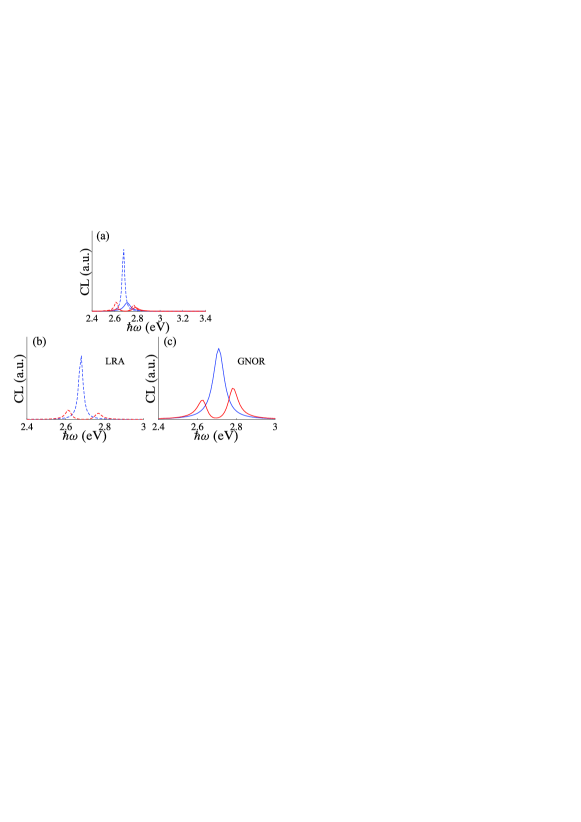
Figure 4: CL spectra and dipolar Rabi-like splitting in plexcitonics, as obtained within LRA and GNOR. All parameters are the same as in Fig. 3. (a) Plasmon–exciton coupling for the dipolar LSP mode. Dashed curves correspond to PE spectra obtained within LRA, while solid curves are the results of the GNOR model. Additionally, blue curves correspond to the PE spectra of the hollow Ag shell, and red curves to those of the excitonic-Ag NP, as in the right-hand schematic of Fig. 1(c). In (b) and (c) we show an enlarged view of the spectra for the LRA and GNOR case, respectively.

V Discussion and conclusion

In summary, we have developed analytic solutions for the EEL and PE probabilities of core-shell NPs in the presence of nonlocal effects, taken into account in the general framework of hydrodynamic models. Applying this formulation to complex core–shell NPs combining a plasmonic and an excitonic component, we showed that EELS and CL are suitable complementary techniques to study strong plasmon–exciton coupling. Focusing in higher-order multipolar LSPs, we showed that it is in principle feasible to achieve strong coupling, and electron microscopies offer a more sensitive means to observe this behaviour.

In the realm of strong plasmon-exciton coupling we have discussed how nonlocal response, as compared to the standard LRA, plays a decisive role in designing the system and determining the spectral features of the involved modes. While nonlocality does not affect the width of the anticrossing, but merely blueshifts both hybrid modes by the same amount, the use of quantum-informed models is necessary when engineering the plasmonic system and choosing the excitonic material. The two components need to be accurately tuned to achieve strong coupling, and the most detailed theoretical predictions of their response can minimize this effort.

In addition to the resonance positions, the more elaborate GNOR model contains additional damping mechanisms. Taking these loss channels into account is fundamental before initiating a quest for strong coupling, as there always lurks the risk that coherent energy exchange between the plasmon and the exciton might prove too slow, and be overcome by absorptive losses, thus preventing entering the strong coupling regime. Nevertheless, we have shown that in the examples studied here, nonlocal damping does not constitute a hindrance, and few-nm NPs could indeed be considered as candidates for electron microscopy-monitored strong coupling.

Concluding, our analytic work should act as a benchmark for the design and theoretical study of more elaborate architectures, while our results should offer further supporting argumentation for turning electron microscopy into a standard tool in the study of strong coupling.

*

Appendix A Derivation of the PE and EEL probabilities in the presence of nonlocal response for core-shell nanospheres

Fig. 5 depicts two set-ups of the core-shell nanoparticle probed by a moving electron. The spherical core has radius $R_{1}$ and the cladding has outer radius $R_{2}$. In both cases, the electron has speed $\nu$ and travels at a distance $d$—the impact parameter—from sphere’s center. The analysis of CL and EEL response due to the two set-ups, enable us to calculate the PE and EEL probabilities. The two set-ups are examined separately.

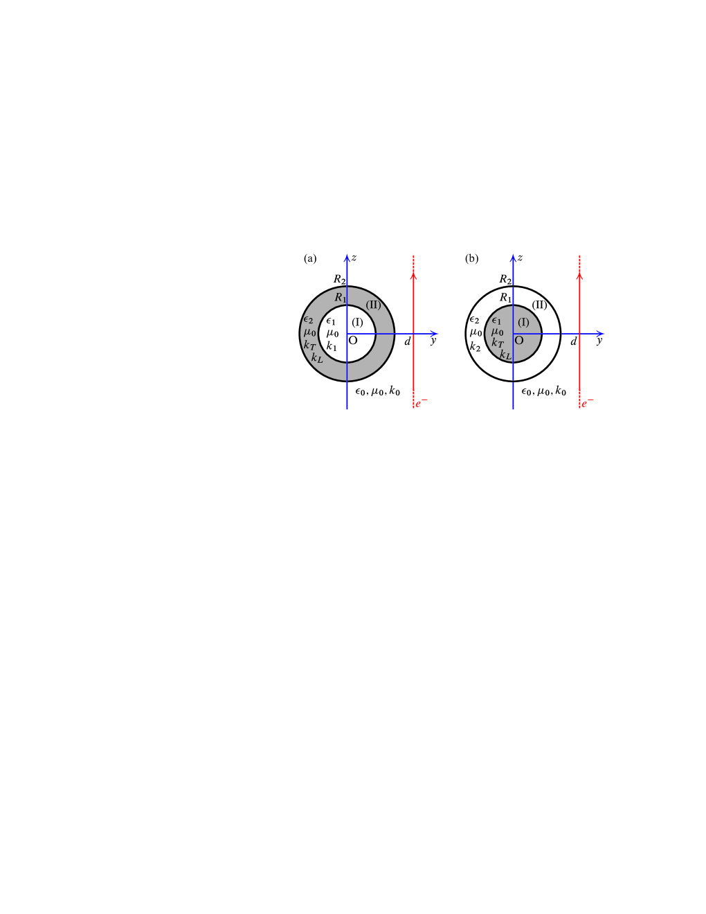
Figure 5: Set-up of core-shell nanospheres probed by electrons. (a) dielectric-metallic configuration. (b) metallic-dielectric configuration.

Dielectric-metallic nanosphere.

Referring to Fig. 5(left), the incident electric field due to a moving electron can be expanded as García de Abajo (1999, 2010)

$${\mathbf{E}}^{\rm inc}({\mathbf{r}})=\sum_{\stackrel{{\scriptstyle\text{\scriptsize$m=-\infty$}}}{{l=|m|}}}^{\infty}\Big{[}a_{lm}\mathbf{M}_{lm}^{(1)}(k_{0},{\mathbf{r}})+b_{lm}\mathbf{N}_{lm}^{(1)}(k_{0},{\mathbf{r}})\Big{]},$$ (4)

where $\mathbf{M}_{lm}^{(1)}$, $\mathbf{N}_{lm}^{(1)}$ are the spherical vector wave functions (SVWFs) of the first kind Chew (1990), $k_{0}=\omega\sqrt{\epsilon_{0}\mu_{0}}$ the free space wavenumber, with $\epsilon_{0}$ and $\mu_{0}$ the free space permittivity and permeability, respectively. Using the $\exp({\rm i}\omega t)$ time dependence, the expansion coefficients in Eq. (4) are given by

$$a_{lm} =\frac{4\pi{\rm i}\omega\nu}{c^{3}}\frac{mA_{lm}^{+}}{l(l+1)}K_{m}\Big{(}\frac{\omega d}{\nu\gamma}\Big{)},$$

$$b_{lm} =\frac{2\pi{\rm i}\omega}{c^{2}\gamma}\frac{B_{lm}^{+}}{l(l+1)}K_{m}\Big{(}\frac{\omega d}{\nu\gamma}\Big{)},$$

$$A_{lm}^{+} =\sqrt{\frac{2l+1}{\pi}\frac{(l-|m|)!}{(l+|m|)!}}(2|m|-1)!!\Big{(}\frac{c}{\nu\gamma}\Big{)}^{|m|}C_{l-|m|}^{|m|+1/2}\Big{(}\frac{c}{\nu}\Big{)},$$

$$B_{lm}^{+} =A_{l,m+1}^{+}\sqrt{(l+m+1)(l-m)}-A_{l,m-1}^{+}\sqrt{(l-m+1)(l+m)}.$$ (5)

In Eq. (A), $\gamma=1/\sqrt{1-\nu^{2}/c^{2}}$, $c$ is the speed of light in vacuum, $K_{m}$ the modified Bessel function, and $C_{n-|m|}^{|m|+1/2}$ the Gegenbauer polynomial. The expansions of the scattered field ${\mathbf{E}}^{\rm s}$ and the field ${\mathbf{E}}^{\rm I}$ inside the dielectric core (region I), are given by

$${\mathbf{E}}^{\rm s}({\mathbf{r}})=\sum_{\stackrel{{\scriptstyle\text{\scriptsize$m=-\infty$}}}{{l=|m|}}}^{\infty}\Big{[}F_{lm}\mathbf{M}_{lm}^{(4)}(k_{0},{\mathbf{r}})+G_{lm}\mathbf{N}_{lm}^{(4)}(k_{0},{\mathbf{r}})\Big{]},$$

$${\mathbf{E}}^{\rm I}({\mathbf{r}})=\sum_{\stackrel{{\scriptstyle\text{\scriptsize$m=-\infty$}}}{{l=|m|}}}^{\infty}\Big{[}A_{lm}\mathbf{M}_{lm}^{(1)}(k_{1},{\mathbf{r}})+B_{lm}\mathbf{N}_{lm}^{(1)}(k_{1},{\mathbf{r}})\Big{]},$$ (6)

with $\mathbf{M}_{lm}^{(4)}$, $\mathbf{N}_{lm}^{(4)}$ the SVWFs of the fourth kind, representing outward travelling waves, while $k_{1}=\omega\sqrt{\epsilon_{1}\mu_{0}}$, $\epsilon_{1}=\epsilon_{1r}\epsilon_{0}$, with $\epsilon_{1r}$ the relative permittivity of the dielectric core. To account for the nonlocal response due to the metallic shell (region II), the field ${\mathbf{E}}^{\rm II}$ must be expanded taking into account longitudinal waves via the $\mathbf{L}_{lm}$ SVWF, i.e.,

$$\!\!\!{\mathbf{E}}^{\rm II}({\mathbf{r}})=\!\!\!\!\!\sum_{\stackrel{{\scriptstyle\text{\scriptsize$m=-\infty$}}}{{l=|m|}}}^{\infty}\Big{[} C_{lm}^{(1)}\mathbf{M}_{lm}^{(1)}(k_{T},{\mathbf{r}})+C_{lm}^{(2)}\mathbf{M}_{lm}^{(2)}(k_{T},{\mathbf{r}})$$

$$+D_{lm}^{(1)}\mathbf{N}_{lm}^{(1)}(k_{T},{\mathbf{r}})+D_{lm}^{(2)}\mathbf{N}_{lm}^{(2)}(k_{T},{\mathbf{r}})$$

$$+E_{lm}^{(1)}\mathbf{L}_{lm}^{(1)}(k_{L},{\mathbf{r}})+E_{lm}^{(2)}\mathbf{L}_{lm}^{(2)}(k_{L},{\mathbf{r}})\Big{]}.$$ (7)

In Eq. (A), $\mathbf{M}_{lm}^{(2)}$, $\mathbf{N}_{lm}^{(2)}$, $\mathbf{L}_{lm}^{(2)}$ are the SVWFs of the second kind. $k_{T}=\omega\sqrt{\epsilon_{2}\mu_{0}}$, with $\epsilon_{2}=\epsilon_{2r}\epsilon_{0}$, is the transverse wavenumber of the LRA of the metallic shell, with the relative dielectric function $\epsilon_{2r}$ following Drude model

$$\epsilon_{2r}(\omega)=\epsilon_{\infty}(\omega)-\frac{\omega_{\rm p}^{2}}{\omega(\omega-{\rm i}\gamma_{\rm m})}.$$ (8)

Here, $\epsilon_{\infty}$ accounts for interband effects, $\omega_{\rm p}$ is the plasma frequency, and $\gamma_{\rm m}$ is the damping rate. The longitudinal wavenumber $k_{L}=\sqrt{\epsilon_{2r}(\omega)}/\xi(\omega)$ depends on the model of nonlocality, either the hydrodynamic or the GNOR model Raza et al. (2015b). For the HDM, $\xi(\omega)\equiv\xi_{\rm H}(\omega)=\beta\sqrt{\epsilon_{\infty}(\omega)}/\sqrt{\omega(\omega-{\rm i}\gamma_{\rm m})}$, with the hydrodynamic parameter $\beta=\sqrt{1/3}v_{\rm F}$ when $\omega\ll\gamma_{\rm m}$, and $\beta=\sqrt{3/5}v_{\rm F}$ when $\omega\gg\gamma_{\rm m}$. In the two latter expressions, $v_{\rm F}$ is Fermi velocity. For the GNOR model, $\xi(\omega)\equiv\xi_{\rm GNOR}(\omega)=\sqrt{\epsilon_{\infty}(\omega)}\sqrt{\beta^{2}+D(\gamma_{\rm m}+{\rm i}\omega)}/\sqrt{\omega(\omega-{\rm i}\gamma_{\rm m})}$, where $D$ is the diffusion constant. Values of $v_{\rm F}$ and $D$ are tabulated for various plasmonic metals Blaber et al. (2009); Raza et al. (2015b); Yang et al. (2015). Corresponding expansions for the magnetic fields ${\mathbf{H}}^{\rm inc}$, ${\mathbf{H}}^{\rm s}$, ${\mathbf{H}}^{\rm I}$, ${\mathbf{H}}^{\rm II}$, are obtained by ${\mathbf{H}}=-\nabla\times{\mathbf{E}}/({\rm i}\omega\mu)$. It is important to note that the magnetic fields do not feature the $\mathbf{L}_{lm}$ SVWF, since $\nabla\times\mathbf{L}_{lm}=0$.

Matching the boundary conditions ${\mathbf{e}}_{r}\times({\mathbf{E}}^{\rm II}-{\mathbf{E}}^{\rm I})=0$, ${\mathbf{e}}_{r}\times({\mathbf{H}}^{\rm II}-{\mathbf{H}}^{\rm I})=0$ on inner surface $r=R_{1}$, ${\mathbf{e}}_{r}\times({\mathbf{E}}^{\rm inc}+{\mathbf{E}}^{\rm s}-{\mathbf{E}}^{\rm II})=0$, ${\mathbf{e}}_{r}\times({\mathbf{H}}^{\rm inc}+{\mathbf{H}}^{\rm s}-{\mathbf{H}}^{\rm II})=0$ on outer surface $r=R_{2}$, as well as the additional boundary conditions ${\mathbf{e}}_{r}\cdot(\epsilon_{\infty}\epsilon_{0}{\mathbf{E}}^{\rm II}-\epsilon_{1r}\epsilon_{0}{\mathbf{E}}^{\rm I})=0$ on $r=R_{1}$ and ${\mathbf{e}}_{r}\cdot(\epsilon_{0}{\mathbf{E}}^{\rm inc}+\epsilon_{0}{\mathbf{E}}^{\rm s}-\epsilon_{\infty}\epsilon_{0}{\mathbf{E}}^{\rm II})=0$ on $r=R_{2}$, to account for the nonlocal effects, we get two separate linear systems for the calculation of the unknown expansion coefficients appearing in Eqs (A) and (A). The first system reads

$$\mathbb{A}\begin{bmatrix}C_{lm}^{(1)}\\ C_{lm}^{(2)}\\ A_{lm}\\ F_{lm}\end{bmatrix}=\begin{bmatrix}0\\ j_{l}(k_{0}R_{2})a_{lm}\\ 0\\ j_{l}^{\rm d}(k_{0}R_{2})/(Z_{0}k_{0}R_{2})a_{lm}\end{bmatrix},$$ (9)

with $\mathbb{A}=(a_{ij})$, $i,j=1,\ldots,4$, and

$$a_{11} =j_{l}(k_{T}R_{1}),a_{12}=y_{l}(k_{T}R_{1}),a_{13}=-j_{l}(k_{1}R_{1}),a_{14}=0,$$

$$a_{21} =j_{l}(k_{T}R_{2}),a_{22}=y_{l}(k_{T}R_{2}),a_{23}=0,a_{24}=-h_{l}^{(2)}(k_{0}R_{2}),$$

$$a_{31} =\frac{j_{l}^{\rm d}(k_{T}R_{1})}{Z_{2}k_{T}R_{1}},a_{32}=\frac{y_{l}^{\rm d}(k_{T}R_{1})}{Z_{2}k_{T}R_{1}},a_{33}=-\frac{j_{l}^{\rm d}(k_{1}R_{1})}{Z_{1}k_{1}R_{1}},a_{34}=0,$$

$$a_{41} =\frac{j_{l}^{\rm d}(k_{T}R_{2})}{Z_{2}k_{T}R_{2}},a_{42}=\frac{y_{l}^{\rm d}(k_{T}R_{2})}{Z_{2}k_{T}R_{2}},a_{43}=0,a_{44}=-\frac{h_{l}^{(2){\rm d}}(k_{0}R_{2})}{Z_{0}k_{0}R_{2}}.$$ (10)

In above relations, $j_{l}$, $y_{l}$, $h_{l}^{(2)}$ is the spherical Bessel, Neumann, Hankel function of the second kind, $z_{l}^{\rm d}(x)\equiv[xz_{l}(x)]^{\prime}_{x}$, $z_{l}\equiv j_{l},y_{l},h_{l}^{(2)}$, and $Z_{0,1,2}=\sqrt{\mu_{0}/\epsilon_{0,1,2}}$. The second linear system is given by

$$\mathbb{B}\begin{bmatrix}D_{lm}^{(1)}\\ D_{lm}^{(2)}\\ E_{lm}^{(1)}\\ E_{lm}^{(2)}\\ B_{lm}\\ G_{lm}\end{bmatrix}=\begin{bmatrix}0\\ j_{l}^{\rm d}(k_{0}R_{2})/(k_{0}R_{2})b_{lm}\\ 0\\ j_{l}(k_{0}R_{2})/Z_{0}b_{lm}\\ 0\\ l(l+1)j_{l}(k_{0}R_{2})/(k_{0}R_{2})b_{lm}\end{bmatrix},$$ (11)

with $\mathbb{B}=(b_{ij})$, $i,j=1,\ldots,6$, while

$$b_{11} =\frac{j_{l}^{\rm d}(k_{T}R_{1})}{k_{T}R_{1}},b_{12}=\frac{y_{l}^{\rm d}(k_{T}R_{1})}{k_{T}R_{1}},b_{13}=\frac{j_{l}(k_{L}R_{1})}{k_{L}R_{1}},b_{14}=\frac{y_{l}(k_{L}R_{1})}{k_{L}R_{1}},b_{15}=-\frac{j_{l}^{\rm d}(k_{1}R_{1})}{k_{1}R_{1}},b_{16}=0,$$

$$b_{21} =\frac{j_{l}^{\rm d}(k_{T}R_{2})}{k_{T}R_{2}},b_{22}=\frac{y_{l}^{\rm d}(k_{T}R_{2})}{k_{T}R_{2}},b_{23}=\frac{j_{l}(k_{L}R_{2})}{k_{L}R_{2}},b_{24}=\frac{y_{l}(k_{L}R_{2})}{k_{L}R_{2}},b_{25}=0,$$

$$b_{26} =-\frac{h_{l}^{(2){\rm d}}(k_{0}R_{2})}{k_{0}R_{2}},$$

$$b_{31} =\frac{j_{l}(k_{T}R_{1})}{Z_{2}},b_{32}=\frac{y_{l}(k_{T}R_{1})}{Z_{2}},b_{33}=0,b_{34}=0,b_{35}=-\frac{j_{l}(k_{1}R_{1})}{Z_{1}},b_{36}=0,$$

$$b_{41} =\frac{j_{l}(k_{T}R_{2})}{Z_{2}},b_{42}=\frac{y_{l}(k_{T}R_{2})}{Z_{2}},b_{43}=0,b_{44}=0,b_{45}=0,b_{46}=-\frac{h_{l}^{(2)}(k_{0}R_{2})}{Z_{0}},$$

$$b_{51} =\epsilon_{\infty}l(l+1)\frac{j_{l}(k_{T}R_{1})}{k_{T}R_{1}},b_{52}=\epsilon_{\infty}l(l+1)\frac{y_{l}(k_{T}R_{1})}{k_{T}R_{1}},b_{53}=\epsilon_{\infty}j^{\prime}_{l}(k_{L}R_{1}),b_{54}=\epsilon_{\infty}y^{\prime}_{l}(k_{L}R_{1}),$$

$$b_{55} =-\epsilon_{1r}l(l+1)\frac{j_{l}(k_{1}R_{1})}{k_{1}R_{1}},b_{56}=0,$$

$$b_{61} =\epsilon_{\infty}l(l+1)\frac{j_{l}(k_{T}R_{2})}{k_{T}R_{2}},b_{62}=\epsilon_{\infty}l(l+1)\frac{y_{l}(k_{T}R_{2})}{k_{T}R_{2}},b_{63}=\epsilon_{\infty}j^{\prime}_{l}(k_{L}R_{2}),b_{64}=\epsilon_{\infty}y^{\prime}_{l}(k_{L}R_{2}),$$

$$b_{65} =0,b_{66}=-l(l+1)\frac{h_{l}^{(2)}(k_{0}R_{2})}{k_{0}R_{2}}.$$ (12)

The prime appearing in $j^{\prime}_{l}$, $y^{\prime}_{l}$ denotes differentiation with respect to the argument.

Once the expansion coefficients of the scattered field are known from the solution of Eqs (9) and (11), the PE probability can be evaluated by García de Abajo (1999); Matyssek et al. (2012b)

$$P_{\rm PE}=\frac{c^{3}}{4\pi^{2}\omega^{3}}\sum_{\stackrel{{\scriptstyle\text{\scriptsize$m=-\infty$}}}{{l=|m|}}}^{\infty}l(l+1)(|F_{lm}|^{2}+|G_{lm}|^{2}),$$ (13)

and the EEL probability by García de Abajo (1999)

$$P_{\rm EEL} =\frac{1}{\pi\omega^{2}}\sum_{\stackrel{{\scriptstyle\text{\scriptsize$m=-\infty$}}}{{l=|m|}}}^{\infty}\Big{\{}m\nu K_{m}\Big{(}\frac{\omega d}{\nu\gamma}\Big{)}{\rm Re}[(A_{lm}^{+})^{\ast}{\rm i}F_{lm}]+\frac{c}{2\gamma}K_{m}\Big{(}\frac{\omega d}{\nu\gamma}\Big{)}{\rm Re}[(B_{lm}^{+})^{\ast}{\rm i}G_{lm}]\Big{\}},$$ (14)

where ${\rm Re}[\cdot]$ represents the real part, and the star denotes complex conjugation.

Metallic-dielectric nanosphere.

In this case, Eq. (4) and ${\mathbf{E}}^{\rm sc}$ in Eq. (A) remain the same, though ${\mathbf{E}}^{\rm I}$ and ${\mathbf{E}}^{\rm II}$ must be expanded as

$$\!\!\!\!\!{\mathbf{E}}^{\rm I}({\mathbf{r}})=\!\!\!\!\!\sum_{\stackrel{{\scriptstyle\text{\scriptsize$m=-\infty$}}}{{l=|m|}}}^{\infty}\Big{[} A_{lm}\mathbf{M}_{lm}^{(1)}(k_{T},{\mathbf{r}})+B_{lm}\mathbf{N}_{lm}^{(1)}(k_{T},{\mathbf{r}})+C_{lm}\mathbf{L}_{lm}^{(1)}(k_{L},{\mathbf{r}})\Big{]},$$

$$\!\!\!\!\!{\mathbf{E}}^{\rm II}({\mathbf{r}})=\!\!\!\!\!\sum_{\stackrel{{\scriptstyle\text{\scriptsize$m=-\infty$}}}{{l=|m|}}}^{\infty}\Big{[} D_{lm}^{(1)}\mathbf{M}_{lm}^{(1)}(k_{2},{\mathbf{r}})+D_{lm}^{(2)}\mathbf{M}_{lm}^{(2)}(k_{2},{\mathbf{r}})+E_{lm}^{(1)}\mathbf{N}_{lm}^{(1)}(k_{2},{\mathbf{r}})+E_{lm}^{(2)}\mathbf{N}_{lm}^{(2)}(k_{2},{\mathbf{r}})\Big{]}.$$ (15)

Now $k_{T}=\omega\sqrt{\epsilon_{1}\mu_{0}}$, $\epsilon_{1}=\epsilon_{1r}\epsilon_{0}$, where $\epsilon_{1r}$ represents the relative permittivity of the plasmonic core and is again given by Drude model of Eq. (8). Furthermore, $k_{L}=\sqrt{\epsilon_{1r}(\omega)}/\xi(\omega)$, and $k_{2}=\omega\sqrt{\epsilon_{2}\mu_{0}}$, $\epsilon_{2}=\epsilon_{2r}\epsilon_{0}$, with $\epsilon_{2r}$ the relative permittivity of the dielectric coating.

Satisfying the additional boundary condition ${\mathbf{e}}_{r}\cdot(\epsilon_{2r}\epsilon_{0}{\mathbf{E}}^{\rm II}-\epsilon_{\infty}\epsilon_{0}{\mathbf{E}}^{\rm I})=0$ on $r=R_{1}$, as well as the remaining boundary conditions for the continuity of the transversal field components, we again get two separate linear systems for the determination of the unknown coefficients. The first system is the same with Eq. (9), but the unknown vector is now $[D_{lm}^{(1)},\;D_{lm}^{(2)},\;A_{lm},\;F_{lm}]^{T}$, whilst $k_{T}$ and $k_{1}$ appearing in $a_{ij}$ of Eq. (9), must be substituted by $k_{2}$ and $k_{T}$, respectively. The second system is now given by

$$\mathbb{B}\begin{bmatrix}E_{lm}^{(1)}\\ E_{lm}^{(2)}\\ B_{lm}\\ C_{lm}\\ G_{lm}\end{bmatrix}=\begin{bmatrix}0\\ j_{l}^{\rm d}(k_{0}R_{2})/(k_{0}R_{2})b_{lm}\\ 0\\ j_{l}(k_{0}R_{2})/Z_{0}b_{lm}\\ 0\end{bmatrix},$$ (16)

with $\mathbb{B}=(b_{ij})$, $i,j=1,\ldots,5$, and

$$b_{11} =\frac{j_{l}^{\rm d}(k_{2}R_{1})}{k_{2}R_{1}},b_{12}=\frac{y_{l}^{\rm d}(k_{2}R_{1})}{k_{2}R_{1}},b_{13}=-\frac{j_{l}^{\rm d}(k_{T}R_{1})}{k_{T}R_{1}},b_{14}=-\frac{j_{l}(k_{L}R_{1})}{k_{L}R_{1}},b_{15}=0,$$

$$b_{21} =\frac{j_{l}^{\rm d}(k_{2}R_{2})}{k_{2}R_{2}},b_{22}=\frac{y_{l}^{\rm d}(k_{2}R_{2})}{k_{2}R_{2}},b_{23}=0,b_{24}=0,b_{25}=-\frac{h_{l}^{(2){\rm d}}(k_{0}R_{2})}{k_{0}R_{2}},$$

$$b_{31} =\frac{j_{l}(k_{2}R_{1})}{Z_{2}},b_{32}=\frac{y_{l}(k_{2}R_{1})}{Z_{2}},b_{33}=-\frac{j_{l}(k_{T}R_{1})}{Z_{1}},b_{34}=0,b_{35}=0,$$

$$b_{41} =\frac{j_{l}(k_{2}R_{2})}{Z_{2}},b_{42}=\frac{y_{l}(k_{2}R_{2})}{Z_{2}},b_{43}=0,b_{44}=0,b_{45}=-\frac{h_{l}^{(2)}(k_{0}R_{2})}{Z_{0}},$$

$$b_{51} =\epsilon_{2r}l(l+1)\frac{j_{l}(k_{2}R_{1})}{k_{2}R_{1}},b_{52}=\epsilon_{2r}l(l+1)\frac{y_{l}(k_{2}R_{1})}{k_{2}R_{1}},b_{53}=-\epsilon_{\infty}l(l+1)\frac{j_{l}(k_{T}R_{1})}{k_{T}R_{1}},$$

$$b_{54} =-\epsilon_{\infty}j^{\prime}_{l}(k_{L}R_{1}),b_{55}=0.$$ (17)

Then, CL spectra and EEL spectra are obtained via Eqs (13) and (14), respectively.