The Sum Composition Problem

Abstract

In this paper, we study the “sum composition problem” between two lists $A$ and $B$ of positive integers. We start by saying that $B$ is sum composition of $A$ when there exists an ordered $m$-partition $[A_{1},\ldots,A_{m}]$ of $A$ where $m$ is the length of $B$ and the sum of each part $A_{k}$ is equal to the corresponding part of $B$. Then, we consider the following two problems: $i)$ the exhaustive problem, consisting in the generation of all partitions of $A$ for which $B$ is sum composition of $A$, and $ii)$ the existential problem, consisting in the verification of the existence of a partition of $A$ for which $B$ is sum composition of $A$. Starting from some general properties of the sum compositions, we present a first algorithm solving the exhaustive problem and then a second algorithm solving the existential problem. We also provide proofs of correctness and experimental analysis for assessing the quality of the proposed solutions along with a comparison with related works.

1 Introduction

The “sum composition problem” between two lists $A=[a_{1},\ldots,a_{n}]$ and $B=[b_{1},\ldots,b_{m}]$ of positive integers consists in the identification of a decomposition of the list $A$ into $m$ sub-lists $A_{1},\ldots,A_{m}$ (where $m$ is the length of $B$) such that the sum of $A_{k}$ is equal to $b_{k}\in B$ ($1\leq k\leq m$). When this decomposition exists we say that $B$ is sum composition of $A$.

The sum composition problem has some analogies and shares the same complexity with the NP-hard number partition problem [4] where a list of integer $A$ is partitioned in $k$ partitions $P_{1}\ldots P_{k}$ such that the sum of each part $P_{j}$ ($1\leq j\leq k$) are as nearly equal as possible. However, there are several practical applications that can be modeled as “sum composition problem”. In the case of weighted graphs, the values in $A$ can correspond to the weights of the edges, and the values in $B$ are the aggregated values according to which the graph should be partitioned. In [8], the sum composition problem is shown as the problem of scheduling independent tasks on uniform machines with different capabilities. In the case of databases, this problem has been encountered by one of the authors when studying functional dependencies in a relational table. Specifically, when a functional dependency between an attribute $x$ and an attribute $y$ of a table $R$ exists, we can consider the list of the occurrences of values assumed by $x$ (denoted $A$) and the corresponding one assumed by $y$ (denoted by $B$). When $B$ is sum composition of $A$ it means that a functional dependency $x\rightarrow y$ can exist (this is a necessary condition but not sufficient). The properties of sum composition can be exploited for simplifying the checking of the existence of a functional dependency by using the statistics associated with the table with no access to the single tuples.

In this paper, we start by interpreting this problem in terms of a partial order relation between two integer partitions [10] and, then, we provide some general properties of such a relation. There are two kinds of properties. Those that guarantee the existence of a sum composition between two lists and those that allow a simplification of the two lists without affecting the property of being one sum composition of the other. These properties are exploited in the realization of two algorithms. The first one, named SumComp, has the purpose to generate all possible decompositions of $A$ for which $B$ is sum composition of $A$. The second one, named SumCompExist, has the purpose to check the existence of at least one decomposition of $A$ for which the relation holds with $B$. In this last case, we are not interested in determining a decomposition but only to verify its existence. The complexity of these algorithms is the same of the algorithms developed for the number partition problem because of the combinatorial explosion of the cases that need to be checked. However, the identified properties and the particular representation of the lists (in which distinct integers are reported along with their multiplicity) allows us to mitigate in some cases the growth of the execution time curve.

As discussed in the related work section, the sum composition problem has received little attention from the research community. However, its formulation can be of interest in many practical applications. Similar problems, presented in the literature for identifying optimal multi-way number partition [9], the k-partitioning problem [8], and the sub-set sum problem [5], usually are devoted to identify a single correspondence between the two lists and sometimes they introduce restrictions on the values occurring in $A$ and $B$. Key characteristics of the proposed approach is the use of different properties of sum composition for reducing the controls in the algorithms and the adoption of a data structure for representing the partitions that reduce the number of combination of values to be considered. As shown in the experimental analysis section, these design strategies have positive effects on the running times of the algorithms (especially for the existential one) even if increasing the size of the partitions the execution times move quickly to an exponential rate.

The paper is structured as follows. Section 2 introduces the problem and some notations. Then, Section 3 deals with the properties of sum composition. Section 4 introduces the SumComp algorithm and proves its correctness. Section 5 revises the previous algorithm for checking the sum composition existence. Section 6 presents the experimental results and Section 7 compares our results with related works. Finally, Section 8 draws the conclusions and future research directions.

2 Problem Definition

An integer partition (or, simply, a partition) of a positive integer $N$ is a list $A=[a_{1},a_{2},\ldots,a_{n}]$ where each part $a_{i}$ is a positive integer, $a_{1}\leq a_{2}\leq\cdots\leq a_{n}$ and $\sigma(A)=a_{1}+a_{2}+\cdots+a_{n}=N$. A partition of $N$ can also be represented as $A=[(a^{\prime}_{1},m_{1}),(a^{\prime}_{2},m_{2}),\ldots,(a^{\prime}_{h},m_{h})]$, where the numbers $a^{\prime}_{1}<\cdots<a^{\prime}_{h}$ are the distinct parts of $A$, and $m_{1},m_{2},\ldots,m_{h}$ are the respective multiplicities. We write $\ell(A)$ for the length of the list $A$, i.e. for the number of parts of the partition $A$, and $\ell^{\prime}(A)$ for the number of distinct parts in $A$. Usually, in the literature, an integer partition is written in decreasing order. In this paper, however, we write an integer partition in increasing order because, as we will see later, this notation is exploited in the formulation of the algorithms.

Example 1.

The list $A\!=\![1,2,2,4,4,6]$ is an integer partition of $N\!=\!\sigma(A)\!=\!19$ with $\ell(A)\!=\!6$ parts and $\ell^{\prime}(A)\!=\!4$ distinct parts. This partition can also be represented as $[(1,1),(2,2),(4,2),(6,1)]$. $\Box$

A decomposition of an integer partition $A=[a_{1},a_{2},\ldots,a_{n}]$ is a list of integer partitions $[A_{1},A_{2},\ldots,A_{m}]$ obtained as follows: given a set partition $\{I_{1},I_{2},\ldots,I_{m}\}$ of the index set $\{1,2,\ldots,n\}$ of $A$, $A_{i}$ is the integer partition whose parts are the $a_{j}$ with $j\in I_{i}$, for $i=1,2,\ldots,m$.

Example 2.

The partition $A=[1,2,2,4,4,6]$ admits, for instance, the decomposition $[A_{1},A_{2},A_{3}]$, where $A_{1}=[1,6]$, $A_{2}=[4]$ and $A_{3}=[2,2,4]$.$\Box$

The set $P_{n}$ of all integer partitions of $n$ can be ordered by refinement [2, pp. 16, 1041] [10] as follows: given two integer partitions $A=[a_{1},a_{2},\ldots,a_{n}]$ and $B=[b_{1},b_{2},\ldots,b_{m}]$, we have $A\leq B$ whenever there exists a decomposition $[A_{1},A_{2},\ldots,A_{m}]$ of $A$ such that $\sigma(A_{i})=b_{i}$, for every $i=1,2,\ldots,m$. The set $P_{n}$ is a very well known poset (partially ordered set) whose topological properties have been studied in several papers (e.g. see [10] and the bibliography therein).

We will say that $B$ is sum composition of $A$ whenever $A\leq B$. Moreover, for simplicity, we will call $AB$-decomposition or enabling decomposition any decomposition of $A$ for which $A\leq B$.

Example 3.

For the two integer partitions $A=[1,2,2,3,4,5]$ and $B=[5,5,7]$, we have the following $AB$-decompositions: $D_{1}=[[2,3],[1,4],[2,5]]$, $D_{2}=[[1,4],[2,3],[2,5]]$, $D_{3}=[[1,2,2],$ $[5],[3,4]]$, $D_{4}=[[2,3],[5],[1,2,4]]$, $D_{5}=[[1,4],[5],[2,2,3]]$, $D_{6}=[[5],[1,2,2],[3,4]]$, $D_{7}=[[5],[2,3],[1,2,4]]$ and $D_{8}=[[5],[1,4],[2,2,3]]$. $\Box$

In this way, the sum composition problem can be formulated as follows:

• generate all the $AB$-decompositions (exhaustive algorithm) between the partitions $A$ and $B$;

• determine if $A\leq B$ (existential algorithm).

The sum composition problem has also a simple puzzle interpretation [7, 10]. Indeed, we have $A\leq B$ whenever there is a tiling of the Ferrers diagram $\Phi_{B}$ of $B$ using the rectangles corresponding to the parts of $A$ (as in Figure 1).

Figure 1: (a) Ferrers diagram $\Phi_{B}$ of the integer partition $B=[2,2,4,7]$. (b) Tiling of $\Phi_{B}$ corresponding to the decomposition $[[1,1],[2],[2,2],[1,3,3]]$ of the integer partition $A=[1,1,1,2,2,2,3,3]$.

Remark 4.

Given an integer partition $B=[b_{1},b_{2},\ldots,b_{m}]$, the number of all $AB$-decompositions with $A\leq B$ is $p(b_{1})p(b_{2})\cdots p(b_{m})$, where $p(k)$ is the number of the integer partitions of $k$ [3, p. 307]. Similarly, given an integer partition $A=[a_{1},\ldots,a_{n}]$, the number of all $AB$-decompositions with $A\leq B$ is at most $b_{n}$, where $b_{n}$ is the Bell number of order $n$ [3, p. 210], i.e. of the number of set partitions of an $n$-set. Finally, given two integer partitions $A=[a_{1},\ldots,a_{n}]$ and $B=[b_{1},b_{2},\ldots,b_{m-1},b_{m}]$ with $A\leq B$, the number $d(A,B)$ of $AB$-decompositions satisfy the bounds $1\leq d(A,B)\leq p(b_{1})p(b_{2})\cdots p(b_{m-1})$. Clearly, if $A=[1,\ldots,1]$ has length $m$ and $B=[m]$, we have $A\leq B$ and $d(A,B)=1$. Moreover, for the partitions $A=[1,1,1,1,1,2,2,3]$ and $B=[2,3,7]$, we have $A\leq B$ and $d(A,B)=6=p(2)p(3)$.

In the rest of the paper, we will use the following operations on integer partitions. The union of two partitions $A$ and $B$ is the partition $A\cup B$ whose parts are those of $A$ and $B$, arranged in increasing order. Similarly, the intersection of $A$ and $B$ is the partition $A\cap B$ whose parts are those common to $A$ and $B$, arranged in increasing order. $A$ is a subpartition of $B$, i.e. $A\subseteq B$, when every part of $A$ is also a part of $B$. If $A$ is a subpartition of $B$, then we write $B\setminus A$ for the partition whose parts are those of $B$ taken off those of $A$. Finally, we write $a\in A$ when $a$ is a part of $A$. In this way, we have $\sigma(A\cup B)=\sigma(A)+\sigma(B)$ and $\sigma(B\setminus A)=\sigma(B)-\sigma(A)$.

Example 5.

Given $A=[1,1,3,4]$ and $B=[1,2,4,4,5]$, we have $A\cup B=[1,1,1,2,3,4,4,4,5]$ and $A\!\cap\!B\!=\![1,4]$. Given $A\!=\![1,1,3,4]$ and $B\!=\![1,1,2,3,3,4,5]$, we have $A\!\subseteq\!B$ and $B\!\setminus\!A\!=\![2,3,5]$. $\Box$

3 Properties of Sum Composition

In this section, we present some properties of the sum composition relation that will be exploited in the exhaustive and existential algorithms presented in the next sections.

3.1 Basic Properties

We start by listing some basic necessary conditions for the existence of a sum composition.

Lemma 6.

Let $A=[a_{1},\ldots,a_{n}]$ and $B=[b_{1},\ldots,b_{m}]$ be two integer partitions such that $A\leq B$, and let $[A_{1},\ldots,A_{m}]$ be an $AB$-decomposition. Then, we have

1. $n\geq m$

2. $a_{1}\leq b_{1}$ (and, more generally, $a_{1}\leq b_{i}$ for every $i$)

3. $a_{n}\leq b_{m}$ (and, more generally, $a_{i}\leq b_{m}$ for every $i$)

4. if $a_{i}\in A_{j}$, then $a_{i}\leq b_{j}$

5. $\sigma(A)=\sigma(B)$.

Proof.

These properties derive directly from the definition of sum composition.

1. Immediate from the definition of the order relation $\leq$.

2. The element $a_{1}$ is the minimum value appearing in $A$. Then $A_{1}$ contains at least one part greater or equal to $a_{1}$ and consequently $b_{1}=\sigma(A_{1})\geq a_{1}$.

3. The element $a_{n}$ is the maximum value appearing in $A$ and appears in some $A_{i}$. Similarly, the element $b_{m}$ is the maximum value appearing in $B$. So, we have $b_{m}\geq b_{i}=\sigma(A_{i})\geq a_{n}$.

4. If $a_{i}\in A_{j}$, then $b_{j}=\sigma(A_{j})=\cdots+a_{i}+\cdots\geq a_{i}$.

5. We have $\sigma(A)=\sigma(A_{1})+\cdots+\sigma(A_{m})=b_{1}+\cdots+b_{m}=\sigma(B)$.

∎

We have also the following useful condition.

Theorem 7.

Let $A=[a_{1},\ldots,a_{n}]$ and $B=[b_{1},\ldots,b_{m}]$ be two integer partitions s.t. $A\leq B$. If the intersection $A\cap B$ has $k$ parts, then $n\geq 2m-k$.

Proof.

Since $A\leq B$, an $AB$-decomposition $[A_{1},\ldots,A_{m}]$ exists. Since $A$ and $B$ have $k$ common parts, there are at most $k$ partitions $A_{i}$ with only one part and all the remaining partitions contains at least two parts. Consequently $n\geq k+2(m-k)=2m-k$. ∎

Remark 8.

By Theorem 7, if $A=[a_{1},\ldots,a_{n}]$ and $B=[b_{1},\ldots,b_{m}]$ are two integer partitions with $A\cap B$ with $k$ parts and $n\leq 2m-k-1$, then $B$ can not be a sum composition of $A$.

The following lemma will be used in the subsequent sections to write the algorithms. It allows you to proceed iteratively on the elements of B, by considering them one by one. The validity of the hypothesis of this lemma is guaranteed at each step.

Theorem 9.

Let $A=[a_{1},\ldots,a_{n}]$ and $B=[b_{1},\ldots,b_{m}]$ be two integer partitions s.t. $\sigma(A)=\sigma(B)$. If $B^{\prime}\!=\!B\!\setminus\![b_{m}]$ is sum composition of some subpartition $A^{\prime}$ of $A$, then $B$ is sum composition of $A$.

Proof.

Since $B^{\prime}$ is sum composition of $A^{\prime}$, there exists an $A^{\prime}B^{\prime}$-decomposition $[A_{1},\ldots,A_{m-1}]$. Let $A_{m}=A\setminus A^{\prime}$. Then $\sigma(A_{m})=\sigma(A)-\sigma(A^{\prime})=\sigma(A)-(\sigma(A_{1})+\cdots+\sigma(A_{m-1}))=\sigma(A)-(b_{1}+\cdots+b_{m-1})=\sigma(A)-(\sigma(B)-b_{m})=b_{m}$. Hence, $[A_{1},\ldots,A_{m-1},A_{m}]$ is an $AB$-decomposition. ∎

Let $A^{(k)}$ be the partition whose parts are the parts of a partition $A=[a_{1},\ldots,a_{n}]$ less or equal to $k$ and let $A^{[k]}$ be the partition whose parts are the parts of $A$ grater or equal to $k$.

Theorem 10.

Let $A=[a_{1},\ldots,a_{n}]$ and $B=[b_{1},\ldots,b_{m}]$ be two integer partitions s.t. $B$ is sum composition of $A$. For every $k=1,\ldots,b_{m}$, we have

$$\sigma(A^{(k)})\geq\sigma(B^{(k)})\qquad\text{and}\qquad\sigma(A^{[k]})\leq\sigma(B^{[k]})\,.$$

Proof.

Since $B$ is sum composition of $A$, there exists an $AB$-decomposition $[A_{1},\ldots,A_{m}]$. If $B^{(k)}=[b_{1},\ldots,b_{h}]$, then $\sigma(A_{1})=b_{1}\leq k$, …, $\sigma(A_{h})=b_{h}\leq k$. Hence, all elements of $A_{1}$, …, $A_{h}$ are less or equal to $k$, and consequently $A_{1}\cup\cdots\cup A_{h}\subseteq A^{(k)}$. Then $\sigma(A^{(k)})\geq\sigma(A_{1})+\cdots+\sigma(A_{h})=b_{1}+\cdots+b_{h}=\sigma(B^{(k)})$.

If $k=1$, we have $A^{[1]}=A$ and $B^{[1]}=B$. So $\sigma(A^{[1]})=\sigma(B^{[1]})$, being $\sigma(A)=\sigma(B)$. If $k>1$, then $A^{[k]}=A\setminus A^{(k-1)}$ and $B^{[k]}=B\setminus B^{(k-1)}$. So $\sigma(A^{[k]})=\sigma(A)-\sigma(A^{(k-1)})\leq\sigma(B)-\sigma(B^{(k-1)})=\sigma(B^{[k]})$. ∎

We have also the following divisibility property (saying, on the other hand, that the sum composition property is preserved by multiplication).

Theorem 11.

Let $A$ and $B$ be two integer partitions s.t. $B$ is sum composition of $A$. If there exists an integer $d>1$ dividing all parts of $A$, then $d$ divides all parts of $B$.

Proof.

Since $A\leq B$, an $AB$-decomposition $[A_{1},\ldots,A_{m}]$ exists. Moreover, by hypothesis, every $a_{i}$ is divisible by $d$, we have at once that each $b_{i}=\sigma(A_{i})$ is divisible by $d$. ∎

Example 12.

Consider the integer partitions $A=[50,100,100,200,250,300]$ and $B=[300,300,400]$. Every element of $A$ and $B$ is divisible by $50$. So, by dividing by 50, we have the partitions $A^{\prime}=[1,2,2,4,5,6]$ and $B^{\prime}=[6,6,8]$. Since $[[6],[1,5],[2,2,4]]$ is an $A^{\prime}B^{\prime}$-decomposition, then $A^{\prime}\leq B^{\prime}$, and consequently $A\leq B$. Notice that to obtain an $AB$-decomposition it is sufficient to multiply all parts of an $A^{\prime}B^{\prime}$-decomposition by $50$. $\Box$

Finally, we have that the sum composition property is preserved by the union of partitions. More precisely, we have the following result.

Theorem 13.

Let $A^{\prime}=[a^{\prime}_{1},\ldots,a^{\prime}_{n^{\prime}}]$, $B^{\prime}=[b^{\prime}_{1},\ldots,b^{\prime}_{m^{\prime}}]$, $A^{\prime\prime}=[a^{\prime\prime}_{1},\ldots,a^{\prime\prime}_{n^{\prime\prime}}]$ and $B^{\prime\prime}=[b^{\prime\prime}_{1},\ldots,b^{\prime\prime}_{m^{\prime\prime}}]$ be four integer partitions s.t. $B^{\prime}$ is sum composition of $A^{\prime}$ and $B^{\prime\prime}$ is sum composition of $A^{\prime\prime}$. Then $B=B^{\prime}\cup B^{\prime\prime}$ is sum composition of $A=A^{\prime}\cup A^{\prime\prime}$.

Proof.

Since $A^{\prime}\leq B^{\prime}$, an $A^{\prime}B^{\prime}$-decomposition $[A_{1}^{\prime},\ldots,A_{m^{\prime}}^{\prime}]$ exists. Similarly, since $A^{\prime\prime}\leq B^{\prime\prime}$, an $A^{\prime\prime}B^{\prime\prime}$-decomposition $[A_{1}^{\prime\prime},\ldots,$ $A_{m^{\prime\prime}}^{\prime\prime}]$ exists. Hence, by properly merging $[A_{1}^{\prime},\ldots,A_{m^{\prime}}^{\prime}]$ and $[A_{1}^{\prime\prime},\ldots,$ $A_{m^{\prime\prime}}^{\prime\prime}]$, we obtain a decomposition of $A^{\prime}\cup A^{\prime\prime}$ for which $A^{\prime}\cup A^{\prime\prime}\leq B^{\prime}\cup B^{\prime\prime}$. ∎

Example 14.

Consider the partitions $A^{\prime}=[1,1,2,3,4]$ and $B^{\prime}=[3,3,5]$ with the $A^{\prime}B^{\prime}$-decomposition $[[1,2],[3],[1,4]]$, and the partitions $A^{\prime\prime}=[1,1,2,3,5]$ and $B^{\prime\prime}=[1,5,6]$ with the $A^{\prime\prime}B^{\prime\prime}$-decomposition $[[1],[1,3],[1,6]]$. Then $A^{\prime}\cup A^{\prime\prime}=[1,1,1,1,2,2,3,3,4,5]$ and $B^{\prime}\cup B^{\prime\prime}=[1,3,3,5,5,6]$, and $[[1],[1,2],[3],[1,4],[2,3],$ $[1,6]]$ is a decomposition of $A^{\prime}\cup A^{\prime\prime}$ for which $A^{\prime}\cup A^{\prime\prime}\leq B^{\prime}\cup B^{\prime\prime}$. $\Box$

Remark 15.

Given two partitions $A$ and $B$ with $A\leq B$, and given two subpartions $A^{\prime}\subseteq A$ and $B^{\prime}\subseteq B$ with $A^{\prime}\leq B^{\prime}$, for the complementary subpartitions $A^{\prime\prime}=A\setminus A^{\prime}$ and $B^{\prime\prime}=B\setminus B^{\prime}$ it is not said that $A^{\prime\prime}\leq B^{\prime\prime}$. Consider, for instance, the partitions $A=[1,1,1,2,2,2,3]$ and $B=[2,2,3,5]$ and the partitions $A^{\prime}=[1,1,2,2,2]\subseteq A$ and $B^{\prime}=[3,5]\subseteq B$. Then $A\leq B$ and $A^{\prime}\leq B^{\prime}$. However, we have $A^{\prime\prime}=[1,3]$ and $B^{\prime\prime}=[2,2]$, and $A^{\prime\prime}\not\leq B^{\prime\prime}$.

3.2 Reduction Properties

In this section, we present some properties that can be used for eliminating values from the partitions involved in a sum composition, without altering the property of being a sum composition. These properties can positively effecting the execution time of the existence algorithm.

Theorem 16.

Let $A=[a_{1},\ldots,a_{n}]$ and $B=[b_{1},\ldots,b_{m}]$ be two integer partitions s.t. $A\leq B$. If two indices $i$ and $j$ exist s.t. $a_{i}=b_{j}$, then $B^{\prime}=[b_{1},\ldots,b_{j-1},$ $b_{j+1},\ldots,b_{m}]$ is sum composition of $A^{\prime}=[a_{1},\ldots,a_{i-1},a_{i+1},\ldots,a_{n}]$.

Proof.

Since $A\leq B$, an $AB$-decomposition $[A_{1},\ldots,A_{m}]$ exists, where, by hypothesis, $a_{i}=b_{j}=\sigma(A_{j})$. We have the following two cases.

1. If $a_{i}\in A_{j}$, then $A_{j}=[a_{i}]$. Hence $[A_{1},\ldots,A_{j-1},A_{j+1},\ldots,A_{m}]$ is an $A^{\prime}B^{\prime}$-decomposition.

2. If $a_{i}\not\in A_{j}$, then there exists an index $k\neq j$ such that $a_{i}\in A_{k}$. Let $A^{\prime}_{k}=(A_{j}\cup A_{k})\setminus[a_{i}]$. Then, replacing $A_{k}$ by $A^{\prime}_{k}$ in $[A_{1},\ldots,A_{j-1},A_{j+1},\ldots,A_{m}]$, we obtain a decomposition of $A^{\prime}$ such that $A^{\prime}\leq B^{\prime}$. Indeed, we have $\sigma(A^{\prime}_{k})=\sigma(A_{j})+\sigma(A_{k})-a_{i}=b_{j}+b_{k}-a_{i}=b_{k}$.

∎

Theorem 16 can be easily generalized as follows.

Theorem 17.

Let $A$ and $B$ be two integer partitions s.t. $B$ is sum composition of $A$. If $C$ is a subpartion of $A$ and $B$, then $B\setminus C$ is sum composition of $A\setminus C$.

Proof.

Suppose that $C=[c_{1},\ldots,c_{k}]$. Since $A$ and $B$ have a common part $c_{1}$, then $B^{\prime}=B\setminus[c_{1}]$ is a sum composition of $A^{\prime}=A\setminus[c_{1}]$, by Theorem 16. Since $A^{\prime}$ and $B^{\prime}$ have a common part $c_{2}$, then $B^{\prime\prime}=B^{\prime}\setminus[c_{2}]$ is a sum composition of $A^{\prime\prime}=A^{\prime}\setminus[c_{2}]$, always by Theorem 16. Continuing in this way, at the end we have that $B\setminus C$ is sum composition of $A\setminus C$. ∎

We also have the following result.

Theorem 18.

If $A$ and $B$ are two partitions s.t. $A\leq B$, then, for every partition $C$, $A\cup C\leq B\cup C$.

Proof.

By hypothesis, we have $A\leq B$, and, clearly, $C\leq C$. Hence, by Theorem 13, we have $A\cup C\leq B\cup C$. ∎

Theorems 17 and 18 immediately implies the following property.

Theorem 19.

If $A$, $B$ and $C$ are three integer partitions, then $A\leq B$ if and only if $A\cup C\leq B\cup C$.

Remark 20.

Equivalently, if $A$ and $B$ are two integer partitions and $C$ is a subpartion of $A$ and $B$, then $A\leq B$ if and only if $A\setminus C\leq B\setminus C$.

Finally, we have the following further simplification property which will be used later to reduce the running time of the existence algorithm.

Theorem 21.

Let $A=[a_{1},\ldots,a_{n}]$ and $B=[b_{1},\ldots,b_{m-1},b_{m}]$ be two integer partitions s.t. $b_{m-1}<a_{n}<b_{m}$. Then $B$ is sum composition of $A$ if and only if $B^{\prime}=[b_{1},\ldots,b_{m-1}]\cup[b_{m}-a_{n}]$ is sum composition of $A^{\prime}=[a_{1},\ldots,a_{n-1}]$.

Proof.

If $A\leq B$, then an $AB$-decomposition $[A_{1},\ldots,A_{m}]$ exists. Suppose that $a_{n}\in A_{k}$. Then, by item 4 of Lemma 6, we have $a_{n}\leq b_{k}$. Hence, being $b_{m-1}<a_{n}<b_{m}$, we have $k=m$, that is $a_{n}\in A_{m}$. Let $A^{\prime}_{m}=A_{m}\setminus[a_{n}]$. Then $[A_{1},\ldots,A_{m-1},A_{m}^{\prime}]$ is a decomposition of $A^{\prime}$ for which $A^{\prime}\leq B^{\prime}$ (indeed, $\sigma(A^{\prime}_{m})=\sigma(A_{m})-a_{n}=b_{m}-a_{n}$).

If $A^{\prime}\leq B^{\prime}$, then an $A^{\prime}B^{\prime}$-decomposition $[A^{\prime}_{1},\ldots,A^{\prime}_{m}]$ exists. If $A^{\prime}_{k}$ corresponds to $b_{m}-a_{n}\in B^{\prime}$, then $[A^{\prime}_{1},\ldots,A^{\prime}_{k-1},A^{\prime}_{k}\cup[a_{n}],A^{\prime}_{k+1},\ldots,A^{\prime}_{m}]$ is an $AB$-decomposition. In fact, for all $A^{\prime}_{i}$ with $i\neq k$ the values are the same, and for $A_{k}=A^{\prime}_{k}\cup[a_{n}]$ we have $\sigma(A_{k})\!=\!\sigma(A^{\prime}_{k})\!+\!a_{n}\!=\!b_{m}\!-\!a_{n}\!+\!a_{n}\!=\!b_{m}$. ∎

Example 22.

Consider $A=[1,1,2,2,4]$ and $B=[1,3,6]$ with $A\leq B$. Since $3<4<6$, for the partitions $A^{\prime}=[1,1,2,2]$ and $B^{\prime}=[1,2,3]$ also holds $A^{\prime}\leq B^{\prime}$. The viceversa is true as well. $\Box$

4 The Exhaustive Sum Composition Algorithm

In this section, we present an algorithm for generating all $AB$-decompositions of two integer partitions $A=[a_{1},\ldots,a_{n}]$ and $B=[b_{1},\ldots,b_{m}]$. To develop such an algorithm, we represent an $AB$-decomposition $[A_{1},\ldots,A_{m}]$ for $B$ as a list $[(b_{1},A_{1}),\ldots,(b_{m},A_{m})]$, where $\sigma(A_{j})=b_{j}$ for every $j=1,\ldots,m$ to better clarify the association between the parts in $B$ and the decomposition of $A$.

1:function SumCompAux($b,A,p$)

2:    if $b<a_{p}$ or $p>\ell^{\prime}(A)$ then return $\emptyset$  end if

3:    $quotient\leftarrow min(b~{}{\tt div}~{}a_{p},m_{p})$ $\triangleright$ Where $(a_{p},m_{p})$ is the $p^{th}$ element of $A$

4:    $Result\leftarrow\emptyset$

5:    for $i\leftarrow 0\ldots quotient$ do

6:        if $i=quotient$ and $quotient\cdot a_{p}=b$ then

7:            $Result=Result\cup\{\{(a_{p},quotient)\}\}$

8:        else

9:            $\{A_{1},\ldots,A_{h}\}\leftarrow\textsc{SumCompAux}(b-ia_{p},A,p+1)$

10:            if $h>0$ then

11:                if $i=0$ then

12:                    $Result=Result\cup\{A_{1},\ldots,A_{h}\}$

13:                else

14:                    $Result=Result\cup\{A_{1}\cup\{(a_{p},i)\},\ldots,A_{h}\cup\{(a_{p},i)\}\}$

15:                end if

16:            end if

17:        end if

18:    end for

19:    return $Result$

20:end function

4.1 The SumCompAux function

Before presenting the general algorithm, we introduce the recursive function SumCompAux having three parameters: an integer partition $A$, an integer $b$ and a position $p$. The purpose of this function is to identify all partitions of the elements of $A$ whose positions are greater (or equal to) $p$ such that their sum is equal to $b$. Of course, when $p=1$ the recursive function SumCompAux identifies all the subpartitions of $A$ such that their sum is $b$.

Example 23.

Consider $A=\{(50,1),(100,2),(200,1),(250,1),(300,1)\}$ and $B=[300,300,400]$ of Example 3. When SumCompAux is called on $A$, a part $b\in B$, and position $1$, we expect that it provides all the subpartitions $A_{1},\ldots,A_{h}$ of $A$ s.t. $\sigma(A_{1})=\ldots=\sigma(A_{h})=b$. Specifically:

• $\textsc{SumCompAux}(300,A,1)\!=\!\{\!\{(50,1),(250,1)\},\!\{(100,1),(200,1)\},\!\{(300,1)\}\!\}$,

• $\textsc{SumCompAux}(400,A,1)=\{\{(50,1),(100,1),(250,1)\},\{(100,2),(200,1)\},\{(100,1),(300,1)\}\}$.

Note that $\textsc{SumCompAux}(300,A,4)=\{\{(300,1)\}\}$. That is, $\{(250,1),(300,1)\}$ are the only parts of $A$ that are considered for determining the value $300$. $\Box$

At each step of the recursion, the function evaluates all the subpartitions of $A$ that can be generated by taking into account the element at position $p$ (denoted $a_{p}$). If $a_{p}$ is greater than $b$ (since $A$ is ordered), no further subpartitions can be determined and the empty set is returned (see Item 3 of Lemma 6). The same conclusion is obtained when the position $p$ is greater than $\ell(A)$. When these cases are not met, it means that $b\geq a_{p}$. Therefore, we can consider the possibility to use $a_{p}$ (or not) in the identification of the subpartitions whose sum is equal to $b$. For this purpose we determine $quotient$ as the minimum between the possible multiplicity of $a_{p}$ (denoted with $m_{p}$) and the integer division of $b$ by $a_{p}$. It represents the maximum number of times that $a_{p}$ can be summed to obtain the value $b$. When the current element is not considered for determining the subpartitions of $A$ whose sum is $b$, the function will return as output the subpartitions that can be determining starting from the element of $A$ of position $p+1$ for the same element $b$. When the current element is taken $i>0$ times, the recursive call is invoked on the value ($b-ia_{p}$) starting from the next position. Therefore, it determines the subpartitions $A_{1},\ldots,A_{h}$ of $A$ whose sum is ($b-ia_{p}$) and will return as output these sets in which element $a_{p}$ is taken $i$ times. When $quotient\cdot a_{p}=b$ there is no needs to proceeds with further recursive calls, and the pair $(a_{p},quotient)$ can be directly returned. Note that, when a call to the recursive function returns the empty set, it means that along this path no results can be obtained.

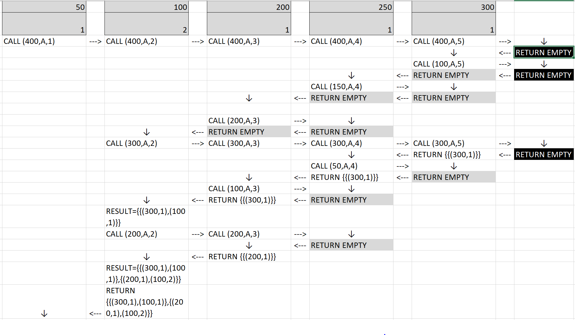
Figure 2: Trace of the execution of function sumCompAux

Example 24.

Figure 2 reports an excerpt of the trace of the calls to function sumCompAux. In the top of the figure the parts of $A$ with their repetitions are shown. The string “return empty” with the black background represents the situation in which we have reached the end of the partition without finding sub-lists whose sum is $b$, whereas the gray background means that it is useless to proceed because $a_{p}>b$. Each column reports all the calls for the same element of $A$.

The first line reports the calls in which the current element of $A$ is not selected. This leads to reach the end of partition $A$ without finding any sub-list of $A$ whose sum is $400$. In returning from the recursive call, the function tries to create a single instance of $300$, and to identify instances of $A$ of position $6$ whose sum is $100$. However, since we have reached the end of $A$, the empty set is returned. The same empty sets are returned in the call backs of the function until the second column (call(300,A,2)) is reached. For this case, indeed, we are able to identify a partition $Result=\{\{(300,1),(100,1)\}\}$. $Result=\{\{(200,1),(100,2)\}\}$ is another subset that is obtained for call(200,A,2). Since we have reached to maximum number of repetitions of $100$ in $A$, the last two results are collected in a partition and returned.

The algorithm proceeds in identifying new results when the part $50$ in $A$ is selected once. We do not further present the other calls, that are analogous to those we have now discussed. $\Box$

The following theorem shows that SumCompAux invoked on $A$, $b$ and position $p$ provides all the partitions $A_{j}$ s.t. $\sigma(A_{j})=b$. This theorem proves that this is true for all $a_{i}\in A$ where $i\geq p$.

Theorem 25.

Let $A=[(a_{1},_{1}),\ldots,(a_{k},m_{k})]$ be a partition, and $b$, $p$ ($p\leq k$) two positive integers. The application of the function SumCompAux to $A$, $b$ and $p$ always terminates and returns all the partitions $A_{1}\subseteq A$, …, $A_{s}\subseteq A$, s.t.:

• the position of the elements in $A_{1}$, …, $A_{s}$ is greater than (or equal to) $p$;

• the sum of the elements in each subpartition is $b$;

• no other subpartitions of $A$ with elements of position greater than (or equal to) $p$ can be identified whose sum is $b$.

Proof.

Let $k=\ell^{\prime}(A)$. We have the following two cases.

Case 1.

If $p>k$, the condition at line 1 guarantees that no solution is provided: an empty set is returned and the function terminates.

Case 2.

If $p\leq k$, we proceed by induction on $q=k-p$.

Case 2.1.

If $q=0$, then $p=k$. In this case, the only element of $A$ to be evaluated is $(a_{k},m_{k})$. The only possible solution is

$$v=b/a_{k}$$ (1)

with $v\leq m_{k}$. We have the following subcases.

Case 2.1.1.

If $b<a_{k}$, then Equation (1) has no solution and the function returns an empty set and terminates (line 2).

Case 2.1.2.

If $b\geq a_{k}$ and Equation (1) has no integer solution or the integer solution is greater than $m_{p}$, then the function returns the empty set. In this case, in fact, no element ($a_{p},t$) with $t\leq m_{p}$ exists s.t. $b=a_{p}t$. The first statement of the else branch (line 9) is executed and the function SumCompAux is called passing a position $p+1>k$. For the part proved in Case 1, the empty set is returned back; therefore the condition at line 10 is false, the empty set is returned and the function terminates.

Case 2.1.3.

If $b\geq a_{k}$ and Equation (1) has an integer solution and the integer solution is lesser or equal than $m_{p}$, then the algorithm provides the set $\{(a_{k},t)\}$ as result which solves exactly Equation 1 with $t\leq m_{k}$ ($k=p$). In fact, in this case, the calculation of $quotient$ gives exactly $t$. In the for loop (line 5) there is only one case that satisfies the condition

$$i=quotient\qquad\text{and}\qquad quotient\cdot a_{p}=b$$ (2)

In this case, when the condition at line 6 is satisfied, the set $\{(a_{k},quotient)\}$ is returned. Otherwise, the else branch (line 8) is executed and, using the same considerations of Case 2.1.2, $Result$ is left unaltered. At the end, the function correctly returns back the set $\{(a_{k},quotient)\}$ and terminates. This closes the proof of Case 2.1

Case 2.2.

If the thesis is true for $q-1$, then we have to prove that it holds also for $q$.

Case 2.2.1.

If $b<a_{p}$, then Equation (1) has no solution neither for position $p$ nor for all positions greater than $p$: the empty set is returned and the function terminates.

Case 2.2.2.

If $b\geq a_{p}$, then we have the solution $A^{\prime}_{j}=[(a_{p},m^{\prime}_{p,j}),\ldots,(a_{k},m^{\prime}_{k,j})]$, where the elements with multiplicity $m^{\prime}_{\_,j}=0$ have been discarded and

$$m^{\prime}_{p,j}\leq m_{p}\qquad\text{and}\qquad b=\sum_{i=p}^{k}m^{\prime}_{i,j}a_{i}$$ (3)

However, the last equation can be rewritten by extracting the part of position $p$ from the sum and moving it to the left member of the equation as follows:

$$b-m^{\prime}_{p,j}a_{p}=\sum_{i=p+1}^{k}m^{\prime}_{i,j}a_{i}\,.$$ (4)

The second member of Equation (4) is the sum of the components of the set $A^{\prime\prime}_{j}=\{(a_{p+1},m^{\prime}_{p+1,j}),\ldots,(a_{k},m^{\prime}_{k,j})\}$. The first member of (4) is formed by varying the $m^{\prime}_{p,j}$ from 0 (when $(a_{p},m^{\prime}_{p,j})$ is not present) to a value $v$, where

$$v\leq b/a_{p}\qquad\text{and}\qquad v\leq m_{p}\,.$$ (5)

The algorithm, after checking the condition at line 2, which is not satisfied, continues with the calculation of $quotient$. $quotient$ is exactly the maximum value as described in (5). The for loop (from line 5 to line 18) spans the $i$ values from 0 to $quotient$.

When $i<quotient$ or $i=quotient$, but $quotient$ is not an exact divisor of $b$, the function enters in the else branch at line 8. In this branch, the set $\{A_{1},\ldots,A_{h}\}$ is calculated by function SumCompAux with parameters $b-ia_{p}$, $A$ and $p+1$ as showed in Equation (4).

Due to the induction hypothesis, with this call, we have returned the set of partitions for position $p+1$ and $b^{\prime}=b-ia_{p}$, as stated in (4) (the $m^{\prime}_{p,j}=i$ and the sum of the elements of the returned set is $b^{\prime}=b-ia_{p}$). If this set is empty for the position $p+1$, it means that no solution exists also for position $p$. If the returned set is not empty, then it is added to $Result$ based on the value of $i$:

• if $i\!=\!0$ by adding the returned set to $\!Result$ as it is because the left member of (4) is $\!b$,

• if $i>0$ we add to the returned set of position $p+1$, also the pair $(a_{p},i)$ because of (4);

Then, we can guarantee that $Result$ contains only and all the correct subpartitions for the case $(a_{p},i)$ with $i<quotient$ or $i=quotient$ but $quotient$ is not an exact divisor of $b$. When $i=quotient$ and $quotient$ is an exact divisor of $b$, then the only possible solution for this case is the pair $(a_{p},quotient)$ ($i=quotient$) because $b=quotient\cdot a_{p}$; then we add to $Result$ the pair $(a_{p},quotient)$. When the for loop ends, the function returns the $Result$ so calculated and terminates the execution. Thus, Case 2.2 is proved.

∎

Algorithm 1 SumComp

1:

2:Input: Two partitions: $A=\{(a_{1},m_{1}),\ldots,(a_{k},m_{k})\}$, $B=[b_{1},\ldots,b_{m}]$

3:Output: The set of all $AB$-decompositions enabling the sum composition from $A$ to $B$ (when the sum composition exists, the empty set otherwise)

4:

5:if $\sigma(A)\not=\sigma(B)$ then return $\emptyset$  end if$\triangleright$ Item 5 of Lemma 6

6:if $m>\ell(A)$ then return $\emptyset$  end if$\triangleright$ Item 1 of Lemma 6

7:if $a_{1}>b_{1}$ or $a_{k}>b_{m}$ then return $\emptyset$  end if$\triangleright$ Item 3 of Lemma 6

8:if $C=A\cap B$ s.t. $\ell(C)>0$ and $\ell(A)\leq 2m-\ell(C)-1$ then return $\emptyset$  end if$\triangleright$ Theorem 7

9:if $\exists b\in B:\sum_{(a_{i},m_{i})\in A\land a_{i}\leq b}m_{i}a_{i}<\sum_{b_{j}\in B\land b_{j}\leq b}b_{j}$ then return $\emptyset$  end if$\triangleright$ Theorem 10

10:$Result\leftarrow\emptyset$

11:if  $m>1$ then

12:    ${\mathcal{A}}\leftarrow\textsc{SumCompAux}(b_{1},A,1)$

13:    if $\mathcal{A}=\emptyset$ then return $\emptyset$  end if

14:    $B^{\prime}\leftarrow B\setminus[b_{1}]$

15:    for each $A_{h}\in{\mathcal{A}}$ do

16:        ${\mathcal{F}}\leftarrow\textsc{SumComp}(A\setminus A_{h},B^{\prime})$

17:        for each $f\in{\mathcal{F}}$ do

18:           $Result\leftarrow Result\cup\{f\cup\{(b_{1},A_{h})\}\}$

19:        end for

20:    end for

21:else

22:    $Result\leftarrow\{\{(b_{1},A)\}\}$

23:end if

24:return $Result$

25:

4.2 The SumComp Algorithm

The function SumCompAux presented in the previous section is the core function of our approach because it generates all possible subpartition $A_{1}$, …, $A_{h}$ of $A$ whose sum is equal to a $b$. If $b$ is the first element of the partition $B$, then each $A_{i}$ ($1\leq i\leq h$) is the first element of an $AB$-decomposition. Moreover, the problem reduces to find all $A^{\prime}B^{\prime}$-decompositions, where $A^{\prime}=A\setminus A_{i}$ ($1\leq i\leq h$) and $B^{\prime}=B\setminus[b_{1}]$.

Starting from this remark, we have developed Algorithm 1 (SumComp) for the generation of all $AB$-decompositions, that works taking into account, in succession, the single elements of $B$. In particular, this algorithm takes advantage of the theoretical results obtained in Section 3.

Algorithm 1 works as follows. First, until line 6, it applies Items 5, 1 and 3 of Lemma 6, and Theorems 7 and 10 for checking necessary conditions of existence of sum composition. When these conditions are met, the algorithm proceeds in the examination of all the elements in $B$, otherwise, we can guarantee that no enabling decompositions can be determined. Then, recursively, the algorithm analyzes the length of $B$. When $\ell(B)=m=1$, all elements of the original $B$ have been analyzed and the pair $(b_{1},A)$ is included in $Result$ (see line 18 of the branch else). Indeed, since the condition at line $2$ is false, it means that $b_{1}$ is the sum of the elements of $A$. When $\ell(B)=m>1$, the function sumCompAux is invoked (line 8) on the first element $b_{1}$ of $B$, the current partition $A$ and the position $1$. In this way, we determine the subpartitions of $A$ whose sum is $b_{1}$. If the result of this invocation is the empty set, it means that no sub-partition $A$ exist whose sum is $b_{1}$ and then the empty set is returned. Otherwise, we have identified all possible subpartition $\mathcal{A}$ for element $b_{1}$, and sumComp is recursively invoked for each of the partition $A_{h}\in\mathcal{A}$ on $A\setminus A_{h}$ and $B\setminus[b_{1}]$. The recursive call will return the decompositions $\mathcal{F}$ for the elements of $B\setminus[b_{1}]$ starting from a partition $A$ from which $A_{h}$ have been removed. At this point, all the elements in $\mathcal{A}$ should be combined with all the elements in $\mathcal{F}$ in order to determine all the $AB$-decompositions between $A$ and $B$ (line 14 of the algorithm).

Figure 3: Recursive calls of the sumComp Algorithm

As shown by the following example, the application of sumComp returns the set $Result$ that contains all the $AB$-decompositions that can be determined from the initial $A$ and $B$.

Example 26.

Let $A=[(50,1),(100,2),(200,1),(250,1),(300,1)]$ and $B=[300,300,400]$ the partition of Example 3. The first line of Figure 3 reports the initial partitions $A$ and $B$. The first vertical arrow on the left leads to the three possible $A_{1}$, $A_{2}$, $A_{3}$ subpartitions whose sum is $300$ (first element of $B$) that can be obtained from $A$ by calling SumCompAux at line 8 of the algorithm. Starting from them, the input of recursive calls to SumComp (line 12) are determined as follows $(A\setminus A_{1},B\setminus[300])$, $(A\setminus A_{2},B\setminus[300])$, and $(A\setminus A_{3},B\setminus[300])$. Then, the second vertical line represents the subpartitions whose sum is $300$ (second element of the initial $B$) that can be obtained from the current $A$. At this point, the backward arrow leads to the partial and final results (in total six) obtained by identifying the subpartitions of $A$ whose sum is $400$. These partial results are accumulated in the $Result$ variable from the recursive calls. The results in green are the new one that are added to the existing ones (in white) in the current step. $\Box$

Theorem 27.

Let $A=[(a_{1},m_{1}),\ldots,(a_{k},m_{k})]$ and $B=[b_{1},\ldots,b_{m}]$ be two partitions. The application of Algorithm 1 to $A$ and $B$ always terminates and returns all possible $AB$-decompositions (the empty set when $A\not\leq B$).

Proof.

Each result $\mathcal{S}_{i}$ of this algorithm has the the form $\mathcal{S}_{i}=\{(b_{1},A_{i,1}),\ldots,$ $(b_{m},A_{i,m})\}$ and is an $AB$-decomposition. To prove this claim we have to show that:

1. $S_{i}$ is an $AB$-decomposition when $A\leq B$, the empty set otherwise.

2. $Result$ contains only $AB$-decompositions.

3. $Result$ contains all $AB$-decompositions.

The algorithm termination is guaranteed by the verification of these three items.

Item 1.

The algorithm first checks if the sufficient conditions of non existence of sum composition (lines 1 to 5) are satisfied. When one of these conditions is true, the empty set is returned and the algorithm terminates. Otherwise, the proof of item 1 is conducted by induction on $m=\ell(B)$

• If $m=1$, then the solution is exactly the partition $A$. In fact, since $m=1$ and the condition of line $1$ is false, we have that $\sum_{i=1}^{k}m_{i}a_{i}=\sum_{j=1}^{m}b_{j}=b_{1}$. $Result$ is initialized with the empty set (line 6) and, since the condition of the if at line 8 is not satisfied, then the instruction at line 18 is executed and assigns to $Result$ the single solution $\{(b_{1},A)\}$.

• We assume the property true for $\ell(B)=m-1$ and we prove it for $\ell(B)=m$. $Result$ is initialized with empty set. The if at line 7 is satisfied, then the invocation of the SumCompAux function returns the set ${\mathcal{A}}$ of all the subpartitions of $A$ whose sum is $b_{1}$, if they exist (see Theorem 25). If ${\mathcal{A}}$ is the empty set (condition at line 9), it means that no combination of elements of $A$ can give as sum $b_{1}$ and then $B$ is not sum composition of $A$ and the empty set is returned. Instead, if ${\mathcal{A}\neq\emptyset}$, then the function spans on all the $A_{h}$ that are the outputs of SumCompAux (from line 11 to line 16). This is to guarantee that each combination of possible solutions is taken into consideration. For each $A_{h}$, the algorithm recursively calculates all the enabling decompositions for $A\setminus A_{h}$ and $B\setminus[b_{1}]$. The two inputs are not empty. In fact, $B\setminus[b_{1}]$ has at least the element $b_{2}$ (being $m>1$). Moreover, $A\setminus A_{h}\neq\emptyset$, being $\sigma(A_{h})=b_{1}<\sigma(B)=\sigma(A)$, i.e. $\sigma(A_{h})<\sigma(A)$. So, by the inductive hypothesis, the set ${\mathcal{F}}$ contains all $A\setminus A_{h},B^{\prime}$-decompositions. The $Result$ is obtained (line 14) by adding, for each solution $f\in{\mathcal{F}}$, the pair $(b_{1},A_{h})$. The obtained result is thus an $AB$-decomposition.

Item 2.

Consider a generic solution in $Result$ and we show that it is valid. The generic solution $s\in Result$, by the induction hypothesis, has the form $s=f\cup\{(b_{1},A_{1})\}$. However, since $f$ is one of the output of Algorithm 1 ($A\setminus A_{1},B\setminus[b_{1}]$), it can be written as $f=\{(b_{2},A_{2}),\ldots,(b_{m},A_{m})\}$. Then $S=\{(b_{1},A_{1})\}\cup\{(b_{2},A_{2}),\ldots,(b_{m},A_{m})\}$ with the property $\sigma(A_{1})=b_{1}$ and $\sigma(A_{i})=b_{i}$ for every $i=2,\ldots,m$. So $A\leq B$.

Item 3.

By absurd, suppose that a solution $S=\{(b_{1},A_{1}),\ldots,(b_{m},A_{m})\}$ is not in $Result$. Because at line 8 we have in ${\mathcal{A}}$ all the pairs ($b_{1},A^{\prime}_{h}$) where $\sigma(A^{\prime}_{h})=b_{1}$ (see Theorem 25), then the pair ($b_{1},A_{1}$) was provided by the function SumCompAux. Then, the recursive call of Algorithm 1 with the parameters $A\setminus A^{\prime}_{1}$ and $B\setminus[b_{1}]$, by inductive hypothesis, returns all $(A\setminus A^{\prime}_{1},B\setminus[b_{1}])$-decompositions. So, it should also contain $\{(b_{2},A_{2}),\ldots,(b_{m},A_{m})\}$. The union of these two sets is thus an $AB$-decomposition, in contradiction with the initial hypothesis.

This concludes the proof of the theorem. ∎

5 The Existential Sum Composition Algorithm

In the previous section, Algorithm 1 was developed for generating all $AB$-decompositions of two given integer partitions $A$ and $B$. However, for several problems (as those mentioned in the introduction) we are not interested on all of them, but only on the fact that $B$ is sum composition of $A$, that is, if there exists at least one $AB$-decomposition. In this section, we develop the Algorithm SumCompExist to provide an answer to such a problem. This algorithm relies on the function SumCompExistAux, which checks the sufficient conditions for having $A\leq B$. This function, however, is invoked only after applying some simplifications, according to the theorems of Section 3.2 for removing elements from $A$ and $B$ while preserving the relation of sum composition.

Algorithm SumCompExist checks in cascade several properties by applying items 1, 3, and 5 of Lemma 6. Then, it applies the first simplification by eliminating the equal values from the partition $A$ and $B$ (Theorem 17). Then, on the returned sets (if not empty) it applies Theorem 7 and then Theorem 21. Finally, it performs the check related to Theorem 10. After these checks and simplifications, the function SumCompExistAux is invoked.

The function SumCompExistAux starts by checking the condition of Item 5 of Lemma 6 (line 12). Whenever the condition is verified, the $false$ value is returned because no $AB$-decompositions can be obtained. Otherwise, the length of $B$ is checked. If $\ell(B)=1$ (line 14), then we are sure that an $AB$-decomposition has been identified. Otherwise, when $\ell(B)>1$, the function (line 14) determines the partitions $[A_{1},\ldots,A_{h}]$ for $b_{1}$ by invoking the function SumCompAux (described in previous section). Whenever $h\not=0$, we have $\sigma(A_{i})=b_{1}$ for every $i=1,\ldots,h$, and, for each $A_{i}$, SumCompExistAux is recursively invoked on $A\setminus A_{i}$ and $B\setminus[b_{1}]$ for checking the relation of sum composition between these two partitions (line 17). When one of these recursive function returns $true$, it means that $A\leq B$ and then the $true$ value is returned (line 18). Whenever none of them returns $true$, it means that no $AB$-decompositions exist and the $false$ value is returned (line 20).

Algorithm 2 SumCompExist

1:

2:Input: Two partitions: $A=\{(a_{1},m_{1}),\ldots,(a_{k},m_{k})\}$, $B=[b_{1},\ldots,b_{m}]$

3:Output: $P=true$ (when the sum composition exists)

4:               $P=false$ otherwise ($B$ is not sum composition of $A$)

5:

6:if $\sigma(A)\not=\sigma(B)$ then return $false$  end if$\triangleright$ Item 5 of Lemma 6

7:if $m>\ell(A)$ then return $false$  end if$\triangleright$ Item 1 of Lemma 6

8:if $a_{1}>b_{1}$ or $a_{k}>b_{m}$ then return $false$  end if$\triangleright$ Item 3 of Lemma 6

9:$(A,B)\leftarrow(A\setminus C,B\setminus C)$ $\triangleright$ Where, $C=A\cap B$ - partition simplification - Corollary 17

10:if $A=\emptyset$ then return $true$  end if$\triangleright$ partitions A and B are equal

11:if $\ell(A)\leq 2\ell(B)-1$ then return $false$  end if$\triangleright$ Theorem 7

12:if $a_{k}\!>\!b_{m-1}$ then $(A,B)\!\leftarrow\!(A\setminus[a_{k}],B\setminus[b_{m}]\cup[b_{m}-a_{k}])$  end if$\triangleright$ Theorem 21

13:if $\!\exists h\!\in\!A\!\cup\!B\!:\!\sum_{(a_{i},m_{i})\in A\land a_{i}\leq h}m_{i}\!\!a_{i}\!<\!\sum_{b_{j}\!\in\!B\land b_{j}\leq h}b_{j}$ then return $false$  end if$\triangleright$ Theorem 10

14:$Result\leftarrow\textsc{SumCompExistAux}(A,B)$

15:return $Result$

16:

17:function SumCompExistAux($A,B$)

18:    if $\sigma(A)\not=\sigma(B)$ then return $false$  end if

19:    if $\ell(A)=1$ then return $true$  end if

20:    $\{A_{1},\ldots,A_{h}\}\leftarrow\textsc{SumCompAux}(b_{1},A,1)$

21:    $B^{\prime}=B\setminus[b_{1}]$

22:    for each $A_{i}\in\{A_{1},\ldots,A_{h}\}$ do

23:        $Result\leftarrow\textsc{SumCompExistAux}(A\setminus A_{i},B^{\prime})$

24:        if $Result=true$ then return $true$  end if

25:    end for

26:    return $false$

27:end function

Example 28.

Let $A=\{(50,1),(100,2),(200,1),(250,1),(300,1)\}$ and $B=[300,300,400]$ be the partitions of Example 3. Since $A\cap B=[300]$, by applying the code at line 4 of the algorithm, we obtain $A=\{(50,1),(100,2),(200,1),(250,1)\}$ and $B=[300,400]$. By considering the first $300$ in $B$, the subpartitions of $A$ whose sum is $300$ are only $\{(50,1),(250,1)\}$ and $\{(100,1),(200,1)\}$. Since the invocation of the recursive function on $A=\{(100,2),(200,1)\}$ and $B=[400]$ returns true, the algorithm returns the existence of a decomposition between the two subpartitions. Therefore, the process in this case is faster than the one described in Example 26. $\Box$

The following theorem provides the correctness of the algorithm.

Theorem 29.

The application of Algorithm SumCompExist to the partitions $A$ and $B$ always terminates and it returns $true$ whenever $B$ is sum composition of $A$.

Proof.

The function SumCompExist can be divided in two parts: the first one (from line 1 to line 9) verifies the sufficient conditions for which $B$ is not sum composition of $A$. The only exceptions are lines 4 and 7 in which the two partitions are simplified. Whenever, after removing from $A$ and $B$ their intersection, the obtained partition $A$ is empty, it means that $A=B$ and trivially $B$ is sum composition of $A$ (line 5).

The second part of SumCompExist is simply returning the result from SumCompExistAux that can be proved by induction on the length of $B$.

Case 1.

If $\ell(B)=1$, then we have two possibilities. If the condition at line 12 is verified, then the function returns $false$ as it has to be by Item 5 of Lemma 6. On the contrary, the condition on line 13 is verified (because $b_{1}=\sigma(A)$) and $true$ is returned. In both cases the algorithm terminates the execution.

Case 2.

If $\ell(B)>1$, we assume true for a $m=\ell(B)-1$, and we prove for $m+1$. Also in this case, if the condition at line 12 is verified, then the function returns $false$ and terminates (according to Item 5 of Lemma 6). The condition at line 13 is false and thus function SumCompAux is invoked on $b_{1}$, $A$, and $1$. It returns the subpartitions $\{A_{1},\ldots,A_{h}\}$ of $A$ s.t. $b_{1}=\sigma(A_{j})$ for every $j=1,\ldots,h$ (Theorem 25). If this set is empty, it means that $b_{1}$ cannot be associated with any element of $A$ and thus $B$ is not sum composition of $A$. Therefore, the function jumps the for loop (lines 16–19), returns $false$ and terminates. On the contrary, if this set is not empty, then the for loop (lines 16–19) is entered and each $A_{i}\in\{A_{1},\ldots,A_{h}\}$ is processed by recursively invoking SumCompExistAux on $A\setminus A_{i}$ and $B\setminus[b_{1}]$. By inductive hypothesis, this function returns the existence of a sum composition between its parameters. When one of the returned value is $true$, the function also returns $true$. Indeed, $\sigma(A_{i})=b_{1}$ and $B\setminus[b_{1}]$ is sum composition of $A\setminus A_{i}$ then, by Lemma 9, $B$ is sum composition of $A$. Whenever none of the recursive invocations of SumCompExistAux returns $true$, it means that $B$ cannot be sum composition of $A$, and the $false$ value is returned and the algorithm terminates.

∎

6 Experimental Results

The algorithms described in the previous sections have been experimentally evaluated by considering synthetic datasets with specific characteristics for comparing their behaviors in the cases in which we know the existence of sum composition and the cases in which no sum composition can be determined. In the generation of the partition $A$, we have considered the possibility to randomly generate $n$ samples in specific ranges of values with or without repetitions. In the following we denote with $A^{n}_{[min,max]}$ the partition $A$ whose length is $n$ and $\forall a\in A,min\leq a\leq max$. For the generation of a partition $B$ with $m$ elements ($\!2\!\leq\!m\!<\!n$) we have considered $\!A^{n}_{[min,max]}\!$ and applied one of the following rules.

1. Randomly split the $A^{n}_{[min,max]}$ in $m$ non-empty partitions and then determine the values of $B$ by summing up the integers in each partition.

2. Generate the sum of the values of $A$, randomly generate $m$ distinct ordered values as follows: $v_{1},\ldots,v_{m-1}$ in the range $[1,\sigma(A)]$, and $v_{m}=\sigma(A)$. Assuming $v_{0}=0$, each $b_{i}$ is obtained as $b_{i}=v_{i}-v_{i-1}$.

Using rule R1, we are guaranteed of the existence of sum composition, whereas by rule R2, we have that $\sigma(A)=\sigma(B)$, but the condition of sum composition is not always guaranteed. Notice that in case of non-existence of a sum composition between the partitions $A$ and $B$, the execution cost of the exhaustive and existential algorithms should be comparable because the entire space of possible solutions has to be explored. In this evaluation, we also wish to study the impact of the properties presented in Section 3 for reducing the number of recursive calls introduced in the algorithms. All experiments have been conducted 100 times for each type of generation of $A$ and $B$ and the reported results (both in terms of execution time and number of enabling decompositions) correspond to their average. The experiments have been executed on a desktop with medium capabilities (Intel Core i7-4790 CPU at 3.60 GHz, processor based on x64 bit, 8 GB RAM).

6.1 Experiments with the SumComp Algorithm

In the evaluation of the performances of the SumComp Algorithm we have considered different combinations of the parameters for the generation of $A^{n}_{[min,max]}$ and the rule $R1$ for the generation of $B$. Indeed, the worst case corresponds on the existence of the sum composition and the need of generating all possible $AB$-decompositions.

The first experiments have been devoted to the identification of the execution time and number of enabling decompositions by varying the length of $A$ and $B$. Due to the explosion of different combinations, and the limitation of the machine used for the experiments, we were able to consider partitions of $A$ with $\ell(A)\leq 23$. Indeed, with $\ell(A)=24$, memory allocation issues were raised ($>4.8$ GB memory used). Moreover, we have considered three ranges of values ($[1,100]$, $[1,150]$, $[1,200]$) in which the values of $A$ have been randomly chosen.

Figure 4 shows a 3-dimensional comparison of the execution times varying the length of $A^{n}_{[1,200]}$ (with $3\leq n\leq 23$) and the length of $B$ (with $2\leq\ell(B)\leq 22$). The range $[1,200]$ has been chosen because it is the most representative among the considered ones, in fact the results in this range dominate the results in the other ones. The graphic shows that the execution times tend to increase when $\ell(B)$ is much smaller than $\ell(A)$. This makes sense because a higher number of possible combinations of values in $A$ can have as sum the values in $B$. The execution times with these examples is affordable, but by increasing of a single unit the length of $A$, the memory is not sufficient for verifying all the different combinations and the results cannot be reported.

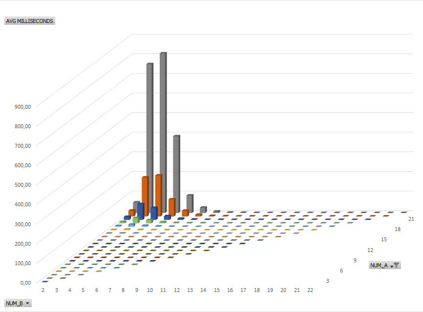
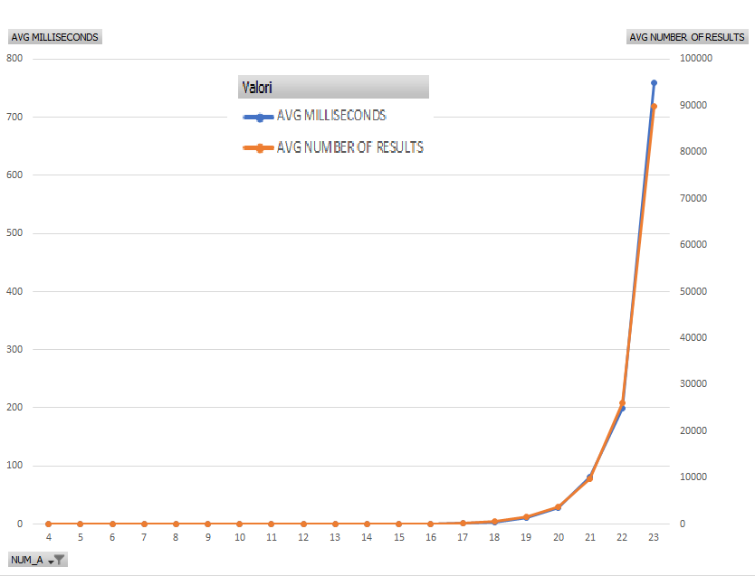
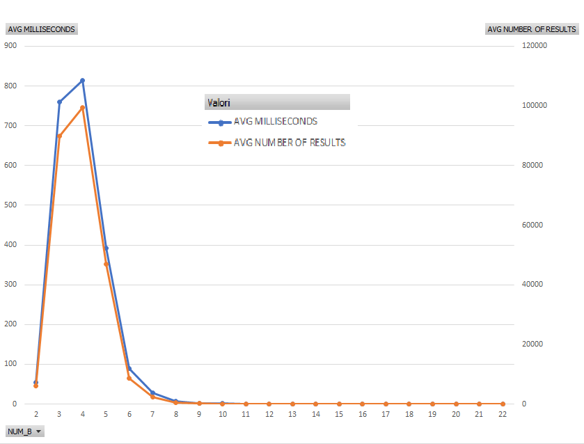
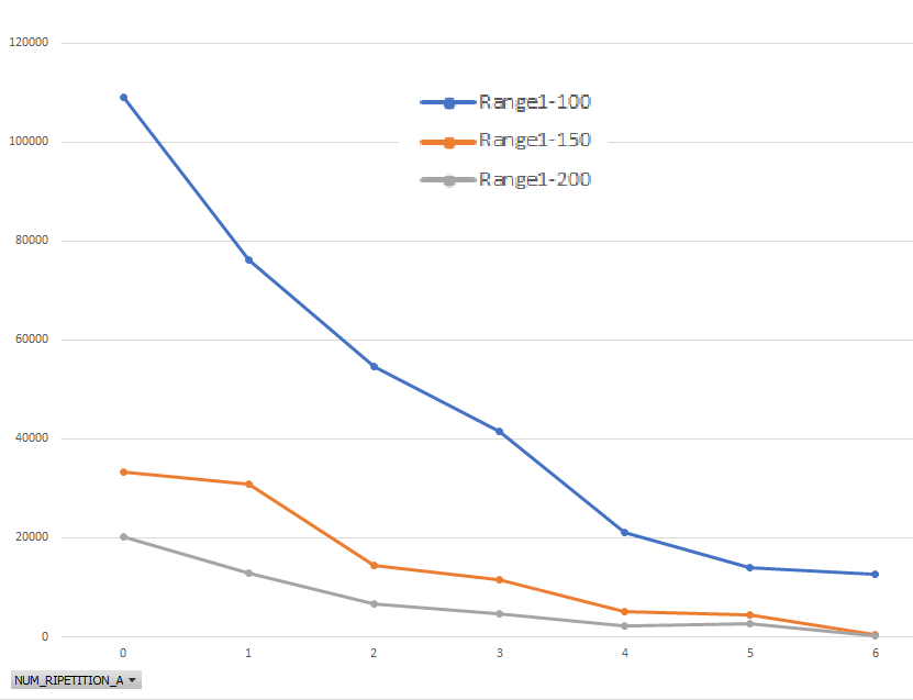
Figure 4: Experiments with function sumComp by applying rule $R1$. $(a)$ Execution times varying the length of $A^{n}_{1,200}$ and $B$ ($1\leq\ell(A),\ell(B)\leq 22$); $(b)$ number of enabling decompositions and execution times varying the length of $A^{n}_{1,200}$ (with $1\leq n\leq 22$) and fixing $\ell(B)=4$; $(c)$ number of enabling decompositions and execution times for $\ell(A)=23$ and varying the length of $B$ ($1\leq\ell(B)\leq 22$); and, $(d)$ execution times with $\ell(A)=23$ and $\ell(B)=2$ varying the number of repetitions in $A$ and the considered ranges ($[1,100]$, $[1,150]$, $[1,200]$).

A slice of Figure 4, by fixing $\ell(B)=4$, is reported in Figure 4 with also the number of identified enabling decompositions. The graphic shows that the number of solutions (as well as the execution times) increase exponentially. Specifically, around $100.000$ enabling decompositions in average can be determined for $\ell(A)=23$ in an elapsed time of 900 ms in average. Moreover, we can identify a correlation between the number of solutions and the execution times (correlation index $\approx 91\%$ on $\ell(A)$). Another slice of Figure 4, by fixing $\ell(A)=23$, is reported in Figure 4. In this case we can note that the maximum execution time (and also the number of enabling decompositions) is obtained for low values of $\ell(B)$. Indeed, the few values contained in $B$ can be obtained by summing different combinations of values in $A$. When $\ell(B)$ increases the possible combinations deeply decrease.

If we now compare all the slices that can be obtained from Figure 4 we can make the following observations. The execution time for the slice corresponding to $\ell(A)=20$ is around $30$ ms while the one for the slice $\ell(A)=23$ moves to $900$ ms with a significant increase of time. Moreover, the highest execution time for the slice corresponding to $\ell(A)=20$ is reached with $\ell(B)=3$, whereas for the case $\ell(A)=23$ the maximum execution time is reached with $\ell(B)=4$. Moreover, in the considered range of values we can state that the maximum number of enabling decompositions follows the law $5.5\leq\frac{\ell(A)}{\ell(B)}\leq 7$. However, this observation holds only for the considered partitions $A$ and ranges. A deeper analysis is required for proving the general validity of this claim. Table 1 reports the number of solutions (in average) by changing the range of values from which the integers in $A$ are chosen. We can observe that the number of enabling decompositions is higher for values of $A$ chosen in the range $[1,100]$. This result is not intuitive and needs further investigations.

# A	Range 1-100	Range 1-150	Range 1-200
18	1,168	447	251
19	4,086	1,520	667
20	13,901	4,261	2,097
21	38,352	18,815	7,810
22	159,581	54,395	26,285
23	477,449	198,690	99,552

Table 1: Number of $AB$-decompositions by varying the length of $A$ and the range of values

Figure 4 shows the impact on the execution time of the presence of repeated elements in $A$. By increasing the number of repetitions of values in $A$ (0 means no duplication, 1 one value duplicated and so on) we observe that the execution time decreases for each range of values. This means that our way to represent partitions has positive impact on the performances.

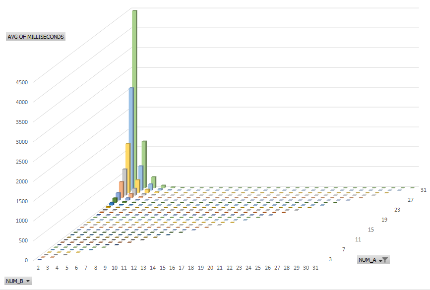
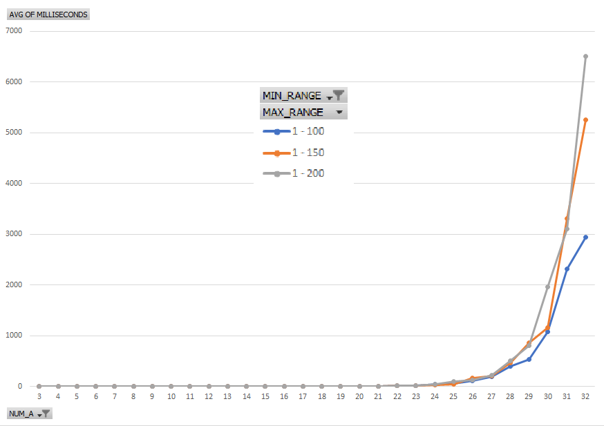
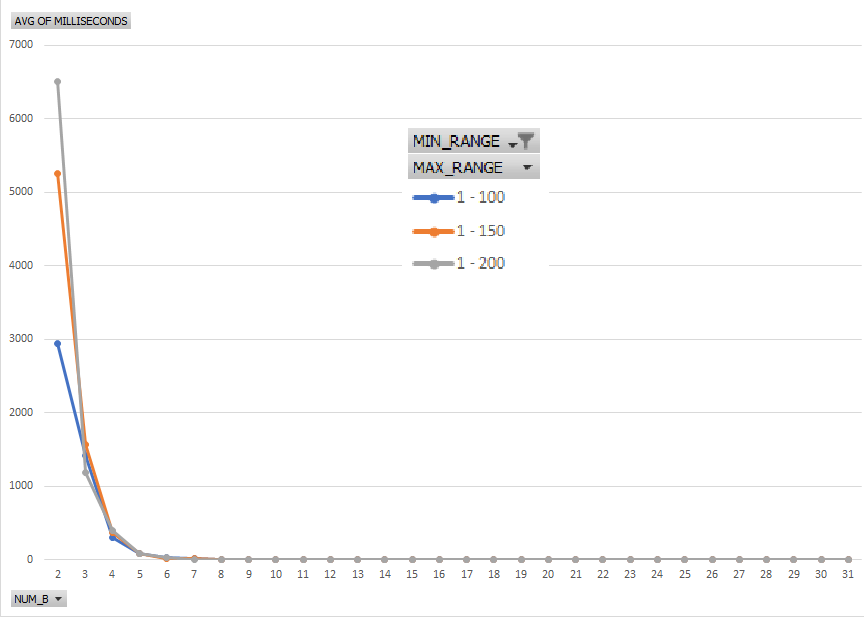
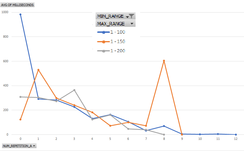
Figure 5: Experiments with function sumCompExist. (a) Execution times varying the length of $A^{n}_{1,200}$ ($3\leq n\leq 32$) and the length of $B$ ($2\leq\ell(B)\leq 31$); (b) number of enabling decompositions and execution times varying the length of $A^{n}_{1,200}$ ($3\leq n\leq 32$) and for $\ell(B)=4$; (c) number of enabling decompositions and execution times for $\ell(A)=32$ and varying the length of $B$ ($2\leq\ell(B)\leq 31$); execution times with $\ell(A)=32$ varying the number of repetitions in $A$ and the considered ranges ($[1,100]$, $[1,150]$, $[1,200]$).

6.2 Experiments with the SumCompExist Algorithm

In the experiments with the existential algorithm we have considered the rule $R2$ for the generation of the partition $B$. Indeed, in this case we are interested in evaluating the behavior of the algorithm also when no solutions exist. Actually, the lack of an enabling decomposition corresponds to the worst case because the entire space of solutions should be explored before reaching to the conclusion. With this algorithm we have identified an issue of lack of memory too (when $\ell(A)=33$). However, since this algorithm does not require to carry all the enabling decompositions, we were able to conduct experiments with a partition $A$ with maximal length of $32$.

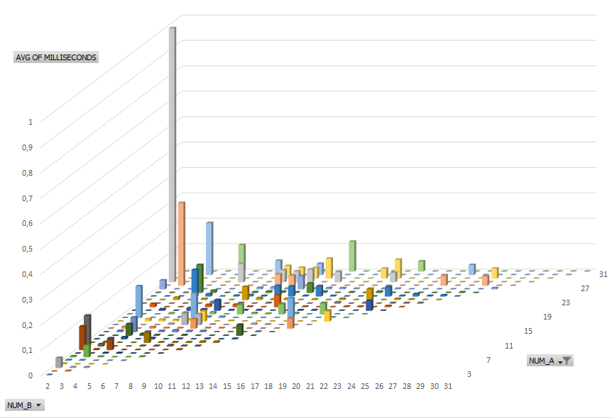
Figure 6: Execution times of sumCompExist when enabling decompositions do not exist – varying the length of $A^{n}_{1,200}$ and the length of $B$ (with $3\leq\ell(A)\leq 32,2\leq\ell(B)\leq 31$)

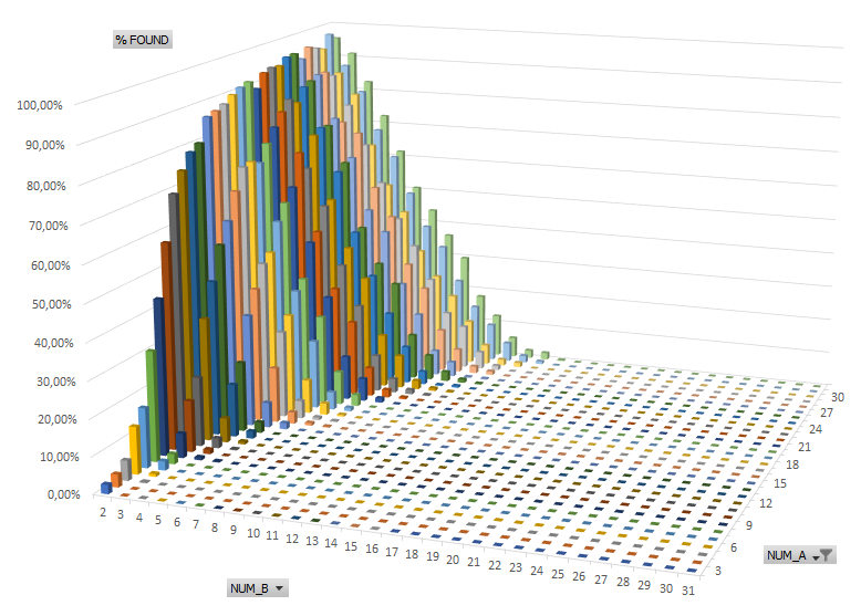
Figure 7: Frequency of existence of sum composition w.r.t. the generated datasets by varying the length of $A^{n}$ for all ranges and the length of $B$ (with $3\leq\ell(A)\leq 32,2\leq\ell(B)\leq 31$)

Figure 5 shows a 3-dimensional comparison of the execution times varying the length of $A^{n}_{[1,200]}$ ($3\leq n\leq 32$) and the length of $B$ ($2\leq\ell(B)\leq 31$). The skyline of the time execution of the existential algorithm is similar to the exhaustive version. However, the absolute times are considerably smaller. Indeed, the worse execution time for the exhaustive algorithm is around 900 ms for $\ell(A)=23$, whereas for the existential algorithm for a partition $A$ with the same length is around $17$ ms. In case of existence, moreover, we are able to handle a partition $A$ with 32 elements. Thus, bigger than those considered in the exaustive case (the average execution time for $\ell(A)=32$ and $\ell(B)=2$ is around $4500$ ms). Analogously to the exhaustive algorithm we have reported some slices of Figure 5 in Figure 5 (by setting $\ell(B)=2$) and in Figure 5 (by setting $\ell(A)=32$) by considering different intervals where the values of $A$ are chosen. The results are analogous with those obtained in the exhaustive algorithm, but we have to observe that the increase in time execution is obtained for higher values of $A$ ($\ell(A)>30$) and that we obtain higher execution times for the range $[1-200]$ and for the case with $\ell(B)=2$.

Figure 5 shows the execution times at increasing number of duplicated values and by considering different ranges of values for $A$. Also in this case we can remark that our representation of partitions has positive effects in the performances of the algorithm. This is more evident for the ranges $[1,100]$ and $[1,200]$, whereas in the range $[1,150]$ we have an outlier (average execution time $4,219$ ms in the case of number of repetitions of elements in $A$ equal to $8$) that has been confirmed by other experiments that we have conducted on the same range of values.

Figure 7 reports the average execution time of the algorithm applied to cases where an enabling decomposition does not exists. These cases have been generated by rule $R2$ discussed at the beginning of the section and considering different lengths of $A$ and $B$ ($\ell(A)$ from $2$ to $32$ elements). It is easy to see that on average the execution time is lesser than 1 ms. By comparing these results with those reported in Figure 5 (where the enabling decompositions always exist) we can observe that identifying the lack of sum composition is much faster than identifying its presence of several order of magnitude. This result is the opposite of what we were expecting. We performed a deeper analysis on these results and we noticed that, for the cases of non existence of sum composition, the simplification mechanisms were very effective by significantly reducing the length of the partitions $A$ and $B$ and, consequently, reducing the execution time of the algorithm

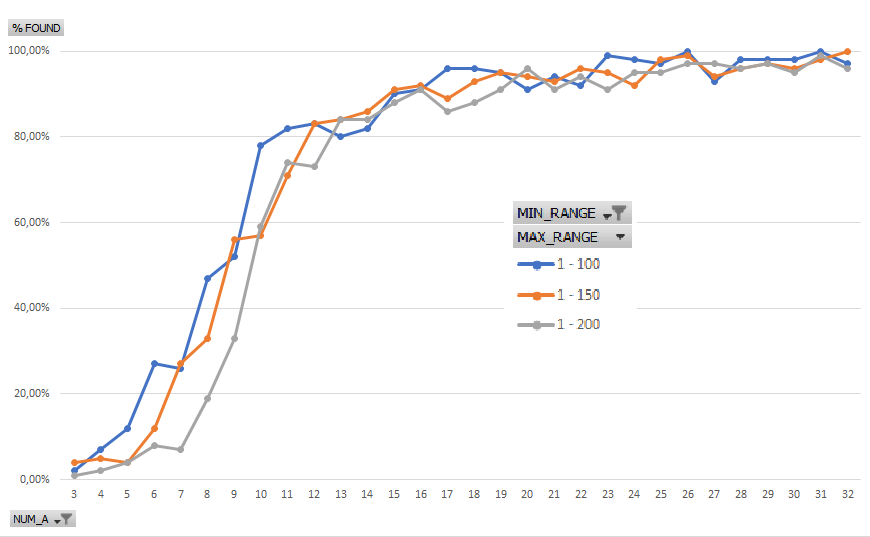
Figure 8: Frequency of existence of sum composition w.r.t. the generated datasets by fixing $\ell(B)=2$ and by varying the length of $A$ for all ranges (with $3\leq\ell(A)\leq 32$)

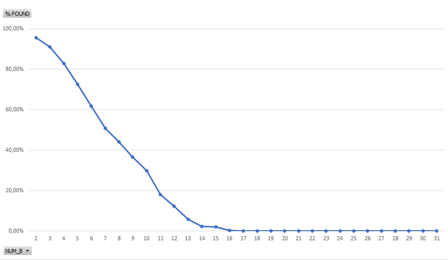
Figure 9: Frequency of lacking of sum composition w.r.t. the generated datasets by fixing $\ell(A)=32$ for all ranges and by varying the length of $B$ (with $2\leq\ell(B)\leq 31$)

Figure 7 reports the frequency of the occurrence of enabling decompositions w.r.t. the number of cases that have been randomly generated in our datasets. The frequency is much higher when the length of $B$ is low (around $2$) and the length of $A$ is high. The trend is better represented in Figure 9 where a slice of the previous figure is shown by fixing $\ell(B)=2$ and in Figure 9 where a slice of previous figure is shown by fixing $\ell(A)=32$. From these graphics we can note that the frequency with which enabling decompositions are identified is $16,56\%$. Moreover, when the ratio $\ell(A)/\ell(B)$ is low, the frequency of cases in which enabling decompositions are not identified rises to $100\%$. The highest numbers of these cases is verified when $\ell(A)/\ell(B)=2$ and this result can be justified by Theorem 7. For higher value of this ratio, it could be worth investigating if the property holds also for higher numbers of $A$.

The last experiments were devoted to evaluate the impact of the simplification properties introduced in Section 3.2 on the performances of the existential algorithm. For this purpose, two kinds of simplifications are considered:

• A full simplification: when the sumCompExist algorithm can decide if the sum composition holds or not without the need to call the SumCompExistAux function. This happens when one of the conditions of the statements 1, 2, 3, 5, 6 and 8 are met in Algorithm 2.

• A partial simplification: when sumCompExist can reduce the execution time of the algorithm by decreasing the numbers of elements of $A$ and $B$ before calling the SumCompExistAux function. This happens when the statements at line 4 or at line 7 is applied.

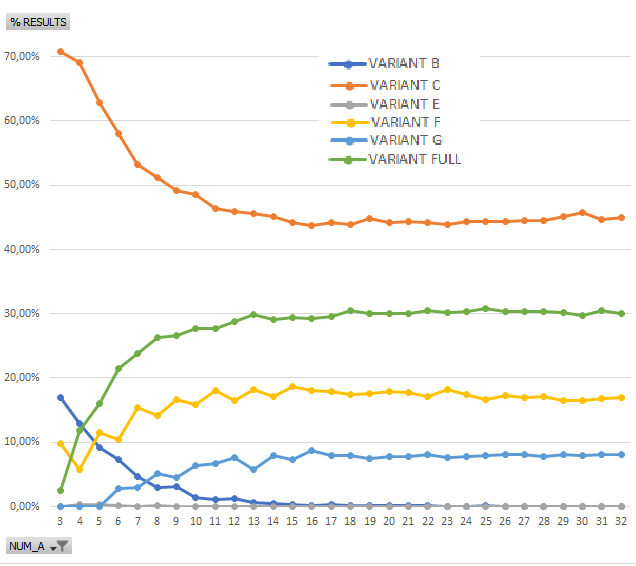
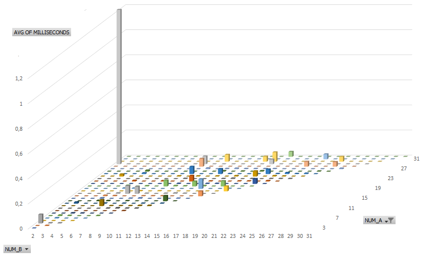
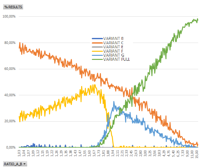
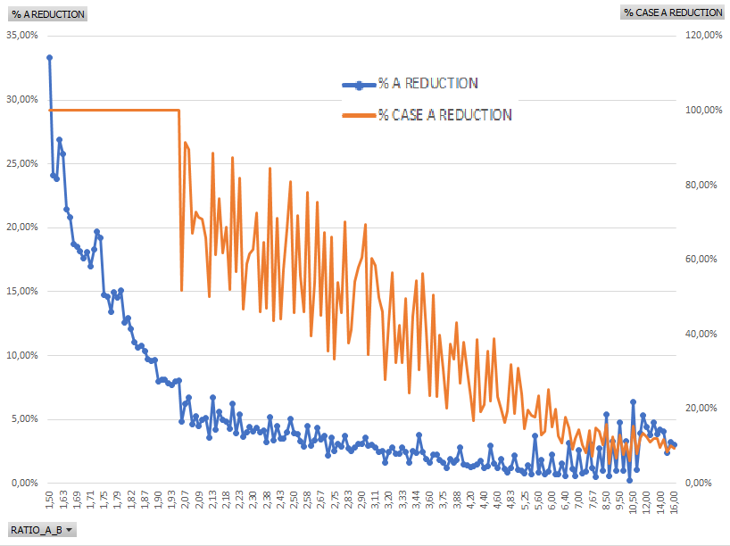
Figure 10: Effect of simplifications on function sumCompExist. (a) Percentage of full simplification variants. (b) average execution time for full simplified variants. (c) Percentage of full simplification variants in relation with the ratio $\ell(A)/\ell(B)$. (d) Percentage of partial simplification on $A$ in relation with the ratio $\ell(A)/\ell(B)$

For the full simplification, the following situations of exit from Algorithm 2 are analyzed:

• variant B. Exit at line 2.

• variant C. Exit at line 3.

• variant E. Exit at line 5.

• variant F. Exit at line 6.

• variant G. Exit at line 8.

These variants are compared with the entire execution of the Algorithm 2 which is denoted variant FULL. Note that the exit at line 1 from Algorithm 2 is not considered because this situation cannot ever be verified because of the use of rule $R2$ in the generation of the datasets.

Figure 10 reports the percentage of cases for the different variants to Algorithm 2. We can see that, for the ranges of values observed, we have that the full simplification can provide the existence or not existence of sum composition for roughly 70% of the cases. This result is quite promising, because despite the high complexity of sum composition, it seems that for a significant percentage of cases, the algorithm can provide an answer quite quickly. The figure shows that the maximum average time is 1.23 ms ($\ell(B)=2$ and $\ell(A)=29$) that is 3 order of magnitude smaller than the case of not full simplification (4,469 ms when $\ell(B)=2$ and $\ell(A)=32$ in Figure 5). Another interesting behavior can be observed in Figure 10: when $\ell(A)\geq 16$ the percentage of full simplification becomes stable for all the cases. This fact deserves further study in the future.

Figure 10 shows the execution times of the different variants w.r.t. the ratio of $\ell(A)$ and $\ell(B)$. We can observe that till the ratio is $3$, this simplification is quite effective in at least 50% of the cases. When this ratio increases, the efficacy of the simplification decreases rapidly. It would be interesting to verify with higher length of $A$ if these results are confirmed. Another investigation direction is to identify other kinds of simplification that can be applied.

Figure 10 shows the effects of partial simplification (only for the call of SumCompExistAux) of the partition $A$ by applying the statements at line 4 and 7 in the sumCompExist algorithm. In particular the line “% CASE A REDUCTION” is the percentage of the cases where we can reduce the number of elements of $A$, line “% A REDUCTION” is the ratio (number of $A$ eliminated)/$\ell(A)$ (two different scales used). The x-axis is the ratio $\ell(A)/\ell(B)$ because it is the most reasonable due the variation of $A$ and $B$ on our tests. We can observe that this kind of simplification is applied in all the cases when $\ell(A)/\ell(B)\leq 2$ then it rapidly decreases arriving at an application of this simplification at roughly 10% of the cases when $\ell(A)/\ell(B)\geq 10$. The percentage of number of $A$ eliminated is even less with a decreasing curve until $\ell(A)/\ell(B)=10$ and then a strange small increase until $\ell(A)/\ell(B)=16$. This kind of simplification can be considered interesting but marginal w.r.t. the most complex cases.

7 Related Work

The sum composition problem, as defined in this article, is hard to find in the literature. A similar class of problems, named Optimal Multi-Way Number Partitioning, can be found in [9]. In their case, the authors provide different optimal algorithms for separating a partition $A$ of $n$ positive integers into $k$ subsets such that the largest sum of the integers assigned to any subset is minimized. The paper provides an overview of different algorithms that fall into three categories: sequential number partitioning (SNP); binary-search improved bin completion (BSIBC); and, cached iterative weakening (CIW). They show experimentally that for large random numbers, SNP and CIW outperform state of the art by up of seven orders of magnitude in terms of runtime. The problem is slightly different from the one that we face in this paper in which we wish to partition the set $A$ according to the values contained in the set $B$. However, we also exploit a SNP approach for the generation of the possible partitions of the partition $A$ according to the integer numbers contained in $B$. Peculiarity of our approach is the representation of the partition $A$ and $B$ that allows one to reduce the cases to be explored by eliminating useless permutations.

A much more similar formulation of the problem faced in this paper is the “k-partition problem” proposed in [8] where the authors wish to minimize a objective function $z$ with the partitions $A$ and $B$ (with the sum of $A$ equals the sum of $B$) where $A$ is partitioned in $m$ subpartitions $(A_{1},\ldots,A_{m})$. For each partition the function $z$ is calculated as $z=max_{i=1}^{m}(\sum_{a\in A_{i}}a)/b_{i}$. It is easy to see that if the minimum of objective function is $z=1$ then $B$ is sum composition of $A$ and, vice versa, if $B$ is sum composition of $A$, the objective function $z=1$. In [8], special restrictions are introduced concerning the length and distinct values of $A$, the maximal integer in $A$ and the minimal integer in $B$ in order to provide more efficient algorithms. For instance, if $\ell(B)=2$ and $max(A)=100$, then $\ell^{\prime}(A)>94$ (i.e. almost all the value from 1 to 100) and $min(B)>2366$. Even if there are many similarities with the approach proposed in this paper, in [8] no real implementation of the algorithms are proposed and the paper lacks of experimental results. Moreover, the paper provides a response to the existence of a solution for the $k$-partition problem but does not provide algorithms for the identification of all possible solutions as we propose in this paper. Finally, our paper provides a characterization of the properties of sum composition that are exploited for reducing the number of cases to be tested. Even if our approach is still NP-hard, its runtime is significantly reduced especially when checking the existence of a solution, and we do not provide any restrictions on the partitions $A$ and $B$.

In our algorithms we need to go through the identification of all the solutions of the well-known “Subset Sum” Problem that is one of Karp’s original NP-complete problems [5]. This problem consists in determining the existence of a subset $A^{\prime}$ of $A$ whose sum is $s$ and is a well-known example of a problem that can be solved in weakly polynomial time. As a weakly NP-complete problem, there is a standard pseudopolynomial time algorithm using a dynamic programming, due to Bellman, that solves it in ${\mathcal{O}}(\ell(A)\sigma(A^{\prime}))$ time [1]. Recently some better solutions have need proposed by Koiliaris and Xuy in [6] with an algorithms that runs in $\tilde{{\mathcal{O}}}(min\{\sqrt{\ell^{\prime}(A)}\sigma(A^{\prime}),\sigma(A^{\prime})^{\frac{4}{3}},\sigma(A)\})$ time, where $\tilde{{\mathcal{O}}}$ hides polylogarithmic factors. We remark that in our case, it is not enough to determine if a subset exists but we need to identify all the possible subsets in $A$ whose sum is $s$. Therefore, the standard approaches proposed in the literature cannnot be directly applied. In our case, we keep the values of $A$ ordered and we apply a SNP approach for enumerating all the possible subpartition of $A$ (starting from the lower values of $A$) that can lead to the sum $s$. A subpartition is skipped when including a new value of $A$, this leads to a value greater that $s$. Since our partitions are ordered, we can guarantee to identify a possible solution, whereas the approach proposed in [6] randomly generates possible configurations to be proved. Finally, relying on our representation of partitions, permutations are avoided and the configurations to test are reduced.

8 Conclusions

In this paper we introduced the sum composition problem between two partitions $A$ and $B$ of positive integers. Starting from a formal presentation of the problem by exploiting the poset theory, we have proposed several properties that can be exploited for improving the execution time of the developed algorithms. Then, we have developed an exhaustive algorithm for the generation of all $AB$-decompositions for which $A\leq B$, and an algorithm for checking the existence of the relation $A\leq B$. The correctness of these two algorithms is proved.

An experimental analysis is provided for assessing the quality of the proposed solutions. As expected, the algorithms have an exponential growth with the length of $A$ and $B$. We also show a correlation between the execution time and the number of enabling decompositions in the execution of the exhaustive algorithm. Moreover, we show that the number of repetitions of the elements in the partition $A$ impacts the execution time for both algorithms and how the adopted data structures reduce the number of configurations to be checked. For the existential algorithm, we had some surprising good impact on “full simplification” actions on roughly $70\%$ of the cases and also “partial simplification” can have good impact in the range of $\ell(A)/\ell(B)\leq 3$. Other interesting experimental evidences were identified as the ratio of $\ell(A)/\ell(B)$ for the enabling decompositions (exhaustive algorithm). Anyway, these algorithms present a limitation of “lack of memory” ($\ell(A)=24$ for the exhaustive algorithm and $\ell(A)=33$ for the existence algorithm).

New area of investigations can be identified in finding: $i)$ new simplification properties that can reduce the execution time of the algorithms; $ii)$ new algorithms that have less limitation of memory usage; $iii)$ a wider range of test cases where the validity of certain properties can be checked.

References

-
[1]
R. Bellman, Notes on the theory of dynamic programming—transportation models,
Manage. Sci. 4 (2) (1958) 191–195.
doi:10.1287/mnsc.4.2.191.
-
[2]
G. Birkhoff, Lattice theory, Vol. 25, American Mathematical Soc., 1940.
-
[3]
L. Comtet, Advanced Combinatorics, Reidel, Boston, 1974.
-
[4]
M. R. Garey, D. S. Johnson, Computers and Intractability: A Guide to the Theory
of NP-Completeness, W. H. Freeman and Co, 1979.
-
[5]
R. M. Karp, Reducibility among Combinatorial Problems, Springer US, 1972,
Ch. 9, pp. 85–103.
-
[6]
K. Koiliaris, C. Xu, A faster pseudopolynomial time algorithm for subset sum,
in: Proc. of the 28th Annual ACM-SIAM SODA, 2017,
pp. 1062–1072.
doi:10.1137/1.9781611974782.68.
-
[7]
S. A. Joni, G.-C. Rota, Coalgebras and bialgebras in combinatorics, Studies in
Applied Mathematics 61 (2) (1979) 93–139.
doi:10.1002/sapm197961293.
-
[8]
C. Mark, Fast exact and approximate algorithms for k-partition and scheduling
independent tasks, Discrete Mathematics 114 (1-3) (1993) 87–103.
-
[9]
E. L. Schreiber, R. E. Korf, M. D. Moffitt, Optimal multi-way number
partitioning, J. ACM 65 (4) (2018) 24:1–24:61.
doi:10.1145/3184400.
- [10] G. M. Ziegler, On the poset of partitions of an integer, Journal of Combinatorial Theory, Series A 42 (2) (1986) 215 – 222. doi:https://doi.org/10.1016/0097-3165(86)90092-0.