Nuclear effects in proton transport and dose calculations

Abstract

Interactions of protons with nuclei are modeled in a form that is suitable for Monte Carlo simulation of proton transport. The differential cross section (DCS) for elastic collisions of protons with neutral atoms is expressed as the product of the Rutherford DCS, which describes scattering by a bare point nucleus, and two correction factors that account for the screening of the nuclear charge by the atomic electrons and for the effect of the structure of the nucleus. The screening correction is obtained by considering the scattering of the projectile by an atom with a point nucleus and the atomic electron cloud described by a parameterization of the Dirac-Hartree-Fock-Slater self-consistent electron density. The DCS for scattering by this point nucleus atom is calculated by means of the eikonal approximation. The nuclear correction to the DCS for elastic collisions is calculated by conventional partial-wave analysis with a global optical-model potential that describes the interaction with the bare nucleus. Inelastic interactions of the projectile with target nuclei are described by using information from data files in ENDF-6 format, which provide cross sections, multiplicities, and angle-energy distributions of all reaction products: light ejectiles (neutrons, protons, …), gammas, as well as recoiling heavy residuals. These interaction models and data have been used in the Monte Carlo transport code penh, an extension of the electron-gamma code penelope, which originally accounted for electromagnetic interactions only. The combined code system penh/penelope performs simulations of coupled electron-photon-proton transport. A few examples of simulation results are presented to reveal the influence of nuclear interactions on proton transport processes and on the calculation of dose distributions from proton beams.

1 Introduction

Monte Carlo simulation is the prime tool for solving radiation transport problems, and finds applications in fields as diverse as microscopy, high-energy physics, radiation metrology and dosimetry, medical physics, and a variety of spectroscopic techniques. Simulations of energetic charged particles are difficult because of the large number of interactions undergone by these particles before being brought to rest. General-purpose Monte Carlo codes for high-energy radiation transport (e.g., etran [1; 2; 3], its3 [4], egs4 [5], geant3 [6], egsnrc [7], mcnp [8], geant4 [9; 10; 11], fluka [12], egs5 [13] mcnp6 [14]) utilize detailed event-by-event simulation for photons, while charged particles are simulated by means of a combination of class I and class II schemes (see Ref. [15]). In class I or condensed simulation schemes, the trajectory of a charged particle is split into segments of predefined length and the cumulative energy loss and angular deflection resulting from the interactions along each segment are sampled from approximate multiple scattering theories. The fluctuation of the energy loss along each segment, is usually accounted for by means of the energy-straggling theories of Landau [16], Blunk and Leisegang [17], or modifications of these theories [18]. Typically, the accumulated angular deflection along a segment is described by means of the multiple-scattering theories of Molière [19], Goudsmit and Saunderson [20; 21], or Lewis [22]. As these theories provide only a partial description of the transport process, they need to be complemented with some sort of approximation to determine the net spatial displacement of the transported particle at the end of the segment, the particle-step transport algorithm [23].

Class II, or mixed, schemes simulate individual hard interactions (i.e., interactions with energy loss $W$ or polar angular deflection $\theta$ larger than certain cut-offs $W_{\rm c}$ and $\theta_{\rm c}$) from their restricted differential cross sections (DCSs), and the effect of the soft interactions (with $W$ or $\theta$ less than the corresponding cut-off) between each pair of hard interactions is described by means of multiple-scattering approximations. Class II schemes not only describe the hard interactions accurately (i.e., according to the adopted DCSs) but also simplify the description of soft events, which have a lesser impact on the transport process. Indeed, by virtue of the central limit theorem, the global effect of a succession of interactions involving only small angular deflections and small energy transfers is nearly Gaussian [24; 25; 26] and it can be described in terms of a few integrals of the DCS restricted to soft interactions.

To the best of our knowledge, penelope [27; 26] is the only general-purpose code that consistently uses class II simulation for all interaction processes of electrons and positrons, while other codes generally use a combination of class I, class II and detailed schemes. In addition, penelope implements a simple tracking scheme (the so-called random-hinge method) that describes spatial displacements fairly accurately. An additional advantage of a class II code is that, when the cut-offs $W_{\rm c}$ and $\theta_{\rm c}$ are set to zero, it performs detailed (event by event) simulations. Since detailed simulation provides an exact reproduction of the transport process conducted by the adopted DCSs (apart from statistical uncertainties), the accuracy of class II simulation can be readily verified by comparing results from detailed and class II simulations of the same arrangement.

The penelope tracking algorithm was also implemented in the proton transport code penh [28] which originally only considered electromagnetic interactions, with atomic nuclei represented as point charges. In the present article we describe physics models and sampling methods that were developed to account for nuclear effects in penh, or in any other class II proton simulation code. We focus on two dominant features that can be included in a class II transport simulation without altering the structure of the code significantly. On the one hand, protons with kinetic energy higher than a few MeV are able to overcome the Coulomb barrier of the nucleus and induce nuclear reactions, which act as a sink for the protons and as a source of energetic reaction products. On the other hand, the finite size and the structure of the nucleus have an effect on the elastic collisions of protons, which alter the DCS at intermediate and large angles by introducing an oscillatory structure.

A detailed microscopic description of the proton-nucleus interaction is not practicable because of the complexity of quantum mechanical and semiclassical treatments. In addition, theoretical calculations of nuclear reactions provide only partial information on the process and in limited energy ranges. Looking for the widest flexibility of the code, we simulate proton-induced nuclear reactions by using information from nuclear databases in the standard ENDF-6 format [29]. These databases provide the reaction cross section $\sigma_{\rm nr}(E)$ and a statistical description of the products emitted in a reaction, as functions of the kinetic energy $E$ of the proton, the average number of released products (prompt gammas, neutrons, protons, deuterons, tritons, ³He, alphas, and residual nuclei), and their angular and energy distributions.

The usual practice in electromagnetic transport simulation codes is to describe elastic collisions by an atomic DCS calculated by considering the target atom as a frozen distribution of electronic charge that screens the Coulomb field of the (point) nucleus. However, the DCS for elastic collisions of protons with atoms is also sensitive to nuclear effects. Although the ENDF-6 files do account for the effect of the finite size and the structure of the nucleus on the elastic DCS, which is described as a correction to the Rutherford DCS, they disregard screening effects. The DCSs adopted in the present study were computed by combining accurate calculations of scattering by the point nucleus screened by the atomic electron cloud and by the bare finite nucleus (by using the same methodology as in the generation of the ENDF-6 files, i.e., conventional partial-wave analysis with a realistic optical-model potential). We have calculated a numerical database of DCSs for elastic scattering of protons by atoms (averaged over naturally occurring isotopes) of the elements with atomic number $Z$ from 1 to 99 and proton kinetic energies between 100 keV and 1 GeV. The proton transport code penh has been modified to account for nuclear effects. The new code simulates elastic collisions by using the numerical DCSs in our database, and it describes nuclear reactions according to the information provided by nuclear databases in the generic ENDF-6 format.

The present article is organized as follows. Section 2 describes the theory and calculations of DCSs for elastic collisions of protons with neutral atoms together with the sampling strategy adopted in the simulation code. An overview of the simulation of inelastic electronic excitations by proton impact, which follows the same scheme as in the previous version of penh [28], is given in Section 3. Section 4 gives a detailed description of the simulation of nuclear reactions based on information from ENDF-6 formatted files. Sample simulation results from penh are presented in Section 5, where the influence of nuclear effects on the dose distributions of proton beams in water is discussed. Finally, we offer our concluding comments in Section 6.

2 Elastic collisions

Let us consider elastic collisions of protons (mass $m_{\rm p}$ and charge $+e$) with atoms of the element of atomic number $Z$. In order to cover the range of proton energies of interest in proton therapy, up to about 300 MeV, we shall use relativistic collision kinematics. The simulation code transports particles in the laboratory (L) frame, where the target atom is at rest and the proton moves with kinetic energy $E$ before the collision. For simplicity, we consider that the $z$ axis of the reference frame is parallel to the linear momentum of the proton, which is given by

$${\bf p}=c^{-1}\sqrt{E(E+2m_{\rm p}c^{2}})\,\hat{\bf z},$$ (1)

where $c$ is the speed of light in vacuum. The total energy of the projectile proton is

$${\cal W}=E+m_{\rm p}c^{2}=\sqrt{m_{\rm p}^{2}c^{4}+c^{2}p^{2}}.$$ (2)

We recall the general relations

$$p=\beta\gamma\,m_{\rm p}c\qquad\mbox{and}\qquad E=(\gamma-1)m_{\rm p}c^{2}$$ (3)

where

$$\beta=\frac{v}{c}=\frac{\sqrt{E(E+2m_{\rm p}c^{2})}}{E+m_{\rm p}c^{2}}$$ (4)

is the speed of the proton in units of $c$ and

$$\gamma=\sqrt{\frac{1}{1-\beta^{2}}}=\frac{E+m_{\rm p}c^{2}}{m_{\rm p}c^{2}}$$ (5)

is the total energy in units of the proton rest energy.

Elastic collisions involve a certain transfer of kinetic energy to the target atom, which is easily accounted for by sampling the collisions in the center-of-mass (CM) frame, which moves with velocity

$${\bf v}_{\rm CM}=\mbox{\boldmath$\beta$}_{\rm CM}c=\frac{c^{2}{\bf p}}{E+m_{\rm p}c^{2}+M_{\rm A}c^{2}},$$ (6)

where $M_{\rm A}$ is the mass of the atom. In the CM frame the linear momenta of the proton and the atom before the collision are, respectively, ${\bf p}^{\prime}_{\rm pi}={\bf p}^{\prime}_{0}$ and ${\bf p}^{\prime}_{\rm Ai}=-{\bf p}^{\prime}_{0}$, with

$${\bf p}^{\prime}_{0}=\frac{M_{\rm A}c^{2}}{\sqrt{(m_{\rm p}c^{2}+M_{\rm A}c^{2})^{2}+2M_{\rm A}c^{2}\;E}}\;{\bf p}.$$ (7)

Quantities in the CM frame are denoted by primes. After the elastic collision, in CM the projectile moves with momentum $p^{\prime}_{\rm pf}=p^{\prime}_{0}$ in a direction defined by the polar scattering angle $\theta$ and the azimuthal scattering angle $\phi$, and the target atom recoils with equal momentum $p^{\prime}_{\rm Af}=p^{\prime}_{0}$ in the opposite direction. The final energies and directions of the proton and the atom in the L frame are obtained by means of a Lorentz boost with velocity $-{\bf v}_{\rm CM}$. Thus, elastic collisions are completely determined by the DCS ${\rm d}\sigma/{\rm d}\Omega^{\prime}$ in the CM frame.

2.1 Interaction potential

In calculations of elastic collisions, the interaction between the projectile proton and the target atom is described by a central potential. The central-potential approximation allows the calculation of the DCS by the conventional partial-wave expansion method, which provides a nominally exact solution of the scattering wave equation. As a first approximation, the atomic nucleus can be considered as a point particle, in which case the interaction potential is

$$V_{\rm scr}(r)=\frac{Ze^{2}}{r}\,\Phi(r)$$ (8)

where $r$ is the distance between the proton and the nucleus and $\Phi(r)$ is the screening function, which accounts for the shielding of the nuclear charge by the atomic electrons. To facilitate calculations, we use approximate screening functions having the analytical form

$$\Phi(r)=\sum_{i=1}^{3}A_{i}\exp(-a_{i}r)\quad\mbox{with}\quad\sum_{i=1}^{n}A_{i}=1,$$ (9)

with the parameters given by [30], which were determined by fitting the self-consistent Dirac-Hartree-Fock-Slater (DHFS) atomic potential of neutral free atoms. The advantage of using this representation of the potential is that a good part of the calculations can be performed analytically. The multiple scattering theory of Molière [31; 19] is based on a parameterization of the DCS calculated with the screening function of Thomas-Fermi atoms approximated in the form (9). Numerical relativistic partial-wave calculations [32] of elastic collisions of electrons and positrons (mass $m_{\rm e}$ and charge $\pm e$) show that the DHFS potential and the analytical approximation (9) yield practically equivalent DCSs for projectiles with kinetic energies higher than about 1 keV.

The interaction of the projectile proton with a bare nucleus of the isotope ${}^{A}Z$ having atomic number $Z$ and mass number $A$ can be described by a phenomenological complex optical-model potential

$$V_{\rm nuc}(r)=V_{\rm opt}(r)+{\rm i}W_{\rm opt}(r),$$ (10)

where the first term is a real potential that reduces to the Coulomb potential at large radii and the second term, ${\rm i}W_{\rm nuc}(r)$, is an absorptive (negative) imaginary potential which accounts for the loss of protons from the elastic channel caused by inelastic processes. Parameterizations of optical-model potentials have been proposed by various authors (see, e.g., Refs. [33; 34; 35]). They are generally written as a combination of Woods–Saxon volume terms,

$$f(R,a;r)=\frac{1}{1+\exp[(r-R)/a]}\,,$$ (11a)

and surface derivative (d) terms,

$$g(R,a;r) = \frac{{\rm d}}{{\rm d}r}\,f(R,a;r)$$ (11b)

$$= \frac{1}{a}\,f(R,a;r)\left[f(R,a;r)-1\right].$$

The parameters in these functions are the radius $R$ and the diffuseness $a$; typically, the radius is expressed as $R=r_{0}A^{1/3}$. We consider a generic potential having the form

$$V_{\rm nuc}(r) = V_{\rm v}(E;r)+V_{\rm d}(E;r)+V_{\rm c}(r)+V_{\rm so}(E;r)\,2\,{\bf L}\!\cdot\!{\bf S}$$ (12)

$$\mbox{}+{\rm i}\left[W_{\rm v}(E;r)+W_{\rm d}(E;r)+W_{\rm so}(E;r)\,2\,{\bf L}\!\cdot\!{\bf S}\rule{0.0pt}{9.95845pt}\right]$$

with the following terms:
1) Real volume potential:

$$V_{\rm v}(E;r)=V_{\rm v}(E)\,f(R_{\rm v},a_{\rm v};r).$$ (13a)

2) Real surface potential:

$$V_{\rm d}(E;r)=V_{\rm d}(E)\,4a_{\rm d}\,g(R_{\rm d},a_{\rm d};r).$$ (13b)

3) Coulomb potential:

$$V_{\rm c}(r)=Ze^{2}\left\{\begin{array}[]{ll}\displaystyle{\frac{1}{2R_{\rm c}}\left(3-\frac{r^{2}}{R_{\rm c}^{2}}\right)}\rule{14.22636pt}{0.0pt}&\mbox{if $r<R_{\rm c}$,}\\[14.22636pt] \displaystyle{\frac{1}{r}}&\mbox{if $r\geq R_{\rm c}$.}\end{array}\right.$$ (13c)

4) Real spin-orbit potential:

$$V_{\rm so}(E;r)=V_{\rm so}(E)\,\frac{1}{r}\,g(R_{\rm so},a_{\rm so};r).$$ (13d)

5) Imaginary volume potential:

$$W_{\rm v}(E;r)=W_{\rm v}(E)\,f(R_{\rm w},a_{\rm w};r).$$ (13e)

6) Imaginary surface potential:

$$W_{\rm d}(E;r)=W_{\rm d}(E)\,4a_{\rm wd}\,g(R_{\rm wd},a_{\rm wd};r).$$ (13f)

7) Imaginary spin-orbit potential:

$$W_{\rm so}(E;r)=W_{\rm so}(E)\,\frac{1}{r}\,g(R_{\rm wso},a_{\rm wso};r).$$ (13g)

The operators $${\bf L} {\bf S} \hbar E$$ and are, respectively, the orbital and spin angular momenta (both in units of ) of the proton. We have indicated explicitly that the strengths of the potential terms are functions (usually expressed as polynomials) of the kinetic energy of the projectile in the L frame.

The interaction energy of the proton with the entire atom is obtained by introducing the screening of the nuclear Coulomb field by the atomic electrons, i.e.,

$$V_{\rm at}(r)=\left[V_{\rm nuc}(r)-V_{\rm c}(r)\right]+V_{\rm c}(r)\,\Phi(r).$$ (14)

The terms in square brackets represent the non-Coulombian nuclear interaction, which has a range of the order of the nuclear radius,

$$R_{\rm nuc}\simeq 1.2\,A^{1/3}\;\mbox{fm.}$$ (15)

The last term is the screened Coulomb interaction that, for $r>R_{\rm nuc}$, reduces to the atomic form and has a range of the order of the “atomic radius”,

$$R_{\rm at}=Z^{-1/3}a_{0},$$ (16)

where $a_{0}=5.29\times 10^{4}$ fm is the Bohr radius.

2.2 Classical equation of motion and wave equation

Let us make a digression to discuss the approximations involved in the calculation of the DCSs in CM. Because nuclear optical-model potentials are determined by requiring that partial-wave calculations yield results consistent with experimental data, we are compelled to assume that the interaction potential $V(r)$ is central. Although this assumption is valid for non-relativistic projectiles, it becomes inconsistent at high energies because the Lorentz-FitzGerald contraction destroys the spherical symmetry of the interaction (see, e.g., Ref. [36]). We present here a brief derivation of the relativistic wave equation for the relative motion of the colliding particles to point out that conventional calculations based on the central-potential approximation not only neglect the asymmetry of the potential but also disregard other components of the effective interaction.

In the CM frame, and assuming a central real potential, the classical equations of motion of the two particles are

$$\dot{\bf p}^{\prime}_{\rm p}={\bf F}\quad\mbox{and}\quad\dot{\bf p}^{\prime}_{\rm A}=-{\bf F}$$ (17)

where ${\bf p}^{\prime}_{\rm p}={\bf p}^{\prime}$ and ${\bf p}^{\prime}_{\rm A}=-{\bf p}^{\prime}$ are the linear momenta of the particles, and

$${\bf F}=-\nabla V(r)=-\frac{{\rm d}V}{{\rm d}r}\,\hat{\bf r},$$ (18)

is the force on the proton (p), which is a function of its position relative to the atom (A), ${\bf r}={\bf r}^{\prime}_{\rm p}-{\bf r}^{\prime}_{\rm A}$. Dotted quantities represent time derivatives. The relative velocity, ${\bf v}=\dot{\bf r}$, is

$${\bf v}={\bf v}^{\prime}_{\rm p}-{\bf v}^{\prime}_{\rm A}=\frac{c^{2}{\bf p}^{\prime}_{\rm p}}{{\cal W}^{\prime}_{\rm p}}-\frac{c^{2}{\bf p}^{\prime}_{\rm A}}{{\cal W}^{\prime}_{\rm A}}=\left(\frac{c^{2}}{{\cal W}^{\prime}_{\rm p}}+\frac{c^{2}}{{\cal W}^{\prime}_{\rm A}}\right){\bf p}^{\prime},$$ (19)

where

$${\cal W}^{\prime}_{\rm p}=\sqrt{m_{\rm p}^{2}c^{4}+c^{2}p^{\prime 2}}\qquad\mbox{and}\qquad{\cal W}^{\prime}_{\rm A}=\sqrt{M_{\rm A}^{2}c^{4}+c^{2}p^{\prime 2}}$$ (20)

are, respectively, the total energies of the proton and the atom.

By virtue of a vis viva theorem, the quantity

$$s\equiv{\cal W}^{\prime}_{\rm p}+{\cal W}^{\prime}_{\rm A}+V(r)$$ (21)

is a constant of motion. Long before the collision, when the distance $r$ is large and $V(r)=0$, $s$ reduces to the total energy in CM, ${\cal W}^{\prime}_{\rm pi}+{\cal W}^{\prime}_{\rm Ai}$, and we can write

$$s^{2}=({\cal W}^{\prime}_{\rm pi}+{\cal W}^{\prime}_{\rm Ai})^{2}-c^{2}({\bf p}^{\prime}_{\rm pi}+{\bf p}^{\prime}_{\rm Ai})^{2},$$ (22)

where the right-hand side is $c^{2}$ times the square of the total four-momentum in CM, a Lorentz invariant. Evaluated with the initial four-momenta in the L frame it reads

$$s^{2}=\left(m_{\rm p}c^{2}+M_{\rm A}c^{2}\right)^{2}+2M_{\rm A}c^{2}E.$$ (23)

As in the non-relativistic study [37], the value of $s$ determines the function $p^{\prime}(r)$ as follows. The equality

$$s-V(r)=\sqrt{m_{\rm p}^{2}c^{4}+p^{\prime 2}c^{2}}+\sqrt{M_{\rm A}^{2}c^{4}+p^{\prime 2}c^{2}}$$ (24)

implies that

$$p^{\prime 2}(r)=\frac{1}{4c^{2}}\left\{\left[s-V(r)\right]^{2}+\frac{(M_{\rm A}^{2}-m_{\rm p}^{2})^{2}c^{8}}{\left[s-V(r)\right]^{2}}\right\}-\frac{(M_{\rm A}^{2}+m_{\rm p}^{2})c^{2}}{2}\,.$$ (25)

With simple rearrangements, this equation can be cast in the familiar non-relativistic form

$$p^{\prime 2}(r)=p^{\prime 2}_{\rm pi}-2\mu_{\rm r}V_{\rm ef}(r)$$ (26)

where

$$\mu_{\rm r}=c^{-2}\frac{{\cal W}^{\prime}_{{\rm pi}}{\cal W}^{\prime}_{{\rm Ai}}}{{\cal W}^{\prime}_{{\rm pi}}+{\cal W}^{\prime}_{{\rm Ai}}}\,.$$ (27)

is the relativistic reduced mass and $V_{\rm ef}(r)$ is an effective potential given by

$$V_{\rm ef}(r)=V(r)+V_{\rm r1}(r)+V_{\rm r2}(r),$$ (28)

with

$$V_{\rm r1}(r)=-\frac{V^{2}(r)}{2\mu_{\rm r}c^{2}}\left(1-\frac{3\mu_{\rm r}c^{2}}{s}\right)$$ (29)

and

$$V_{\rm r2}(r)=\frac{(m_{\rm p}^{2}-M_{\rm A}^{2})^{2}c^{6}}{8\mu_{\rm r}s^{2}}\left[\left(1-\frac{V(r)}{s}\right)^{-2}-1-2\frac{V(r)}{s}-3\frac{V^{2}(r)}{s^{2}}\right].$$ (30)

The terms $V_{\rm r1}(r)$ and $V_{\rm r2}(r)$ are corrections to the interaction potential that account for the effect of relativistic kinematics. The first term is always attractive and proportional to $V^{2}(r)$. Considering the Taylor expansion of the function $(1-x)^{-2}$, one sees that the second correction term, $V_{\rm r2}(r)$, is of order $(V/s)^{3}$, and it vanishes when the projectile and the target particles have the same mass.

The quantum wave equation governing the motion of the projectile relative to the target atom can be obtained from the classical equation 26, by introducing the replacement ${\bf p}^{\prime}\rightarrow-{\rm i}\hbar\nabla$, and considering that the resulting operators act on the wave function $\psi({\bf r})$ (see, e.g., Ref. [38]). We thus find the time-independent wave equation for free states

$$\left(-\frac{\hbar^{2}}{2\mu_{\rm r}}\,\nabla^{2}+V_{\rm ef}(r)\right)\psi({\bf r})=\frac{p^{\prime 2}_{0}}{2\mu_{\rm r}}\,\psi({\bf r})\,,$$ (31)

which has the same form as the non-relativistic Schrödinger equation for scattering of a particle with the relativistic reduced mass $\mu_{\rm r}$ and linear momentum $p^{\prime}_{0}$ by the potential $V_{\rm ef}(r)$. Hence, the wave function $\psi({\bf r})$ and the scattering DCS can be evaluated using the methods and approximations of non-relativistic quantum theory. This formulation ensures that the calculated DCS approximates the well-known classical result [39; 37] in the limit where classical mechanics is valid.

To justify the wave equation (31), let us assume for a moment that the interaction is purely electrostatic. When the mass $M_{\rm A}$ of the target atom tends to infinity, $\beta_{\rm CM}\simeq 0$ and the CM frame coincides with the L frame, where the potential is strictly central. Under these circumstances, ${\bf p}^{\prime}_{0}={\bf p}$, $s\simeq\infty$,

$$\mu_{\rm r}\simeq c^{-2}{\cal W}^{\prime}_{pi}=\gamma m_{\rm p},\quad\mbox{with}\quad\gamma=\sqrt{1+\left(\frac{p^{\prime}_{0}}{m_{\rm p}c}\right)^{2}}\,,$$ (32)

$$V_{\rm ef}(r)=V(r)\left[1-\frac{V(r)}{2\gamma m_{\rm p}c^{2}}\right],$$ (33)

and the wave equation becomes

$$\left(-\frac{\hbar^{2}}{2\gamma m_{\rm p}}\,\nabla^{2}+V(r)\left[1-\frac{V(r)}{2\gamma m_{\rm p}c^{2}}\right]\right)\psi({\bf r})=\frac{p^{\prime 2}_{0}}{2\gamma m_{\rm p}}\,\psi({\bf r}),$$ (34)

which, as expected, coincides with the Klein-Gordon (or relativistic Scrödinger) equation for free states of a proton with initial momentum $p^{\prime}_{0}$ in the electrostatic potential $V(r)$ (see, e.g., Ref. [40]). Our derivation shows that the second term in the effective Klein-Gordon potential (33) has a purely kinematic origin.

It is worth noticing that, in the energy range of interest for transport calculations, the de Broglie wavelengths, $\lambda_{\rm dB}=h/p^{\prime}_{0}$, of protons is much smaller than the atomic radius $R_{\rm at}$. The values of $\lambda_{\rm dB}$ for protons with kinetic energies of 1 MeV and 100 MeV are, respectively, 4.5 fm and 0.44 fm. As a consequence, the numerical solution of the radial wave equation that determines the phase-shifts is very difficult. In addition, the partial-wave series converge extremely slowly, requiring the calculation of a large number ($\gtrsim 100,000$) of phase-shifts. Since approximate calculation methods are available for the case of screened Coulomb potentials (i.e., corresponding to atoms with a point nucleus), we shall consider screening and nuclear effects separately by using the most accurate calculation methods that are practicable for each case.

2.3 Electronic screening

In the case of scattering of energetic protons by screened atomic potentials of the type given by Eq. (8), the relativistic correction terms $V_{\rm r1}(r)$ and $V_{\rm r2}(r)$, Eqs. (29) and (30), decrease rapidly when $r$ increases. The corresponding DCS is strongly peaked at small angles, which correspond to large impact parameters, at which the correction terms are much smaller than the potential $V(r)$. Numerical calculations show that the effect of these correction terms on the DCS is limited to large angles (larger than about 50 degrees for protons with energies up to 1 GeV), where the DCS is more than ten orders of magnitude smaller than at forward angles. Hence, for the purposes of proton transport simulations [31; 28], the DCS for the potentials 5 can be calculated from the wave equation (31) with $V_{\rm eff}(r)=V_{\rm scr}(r)$,

$$\left(-\frac{\hbar^{2}}{2\mu_{\rm r}}\,\nabla^{2}+V_{\rm scr}(r)\right)\psi({\bf r})=\frac{p^{\prime 2}_{0}}{2\mu_{\rm r}}\,\psi({\bf r})\,.$$ (35)

It is worth noticing that, within this scheme, the definition (27) of $\mu_{\rm r}$ accounts for the correct relativistic kinematics. Here we are disregarding the effect of the spin of the proton, which is appreciable only at large scattering angles; it will be accounted for in the calculation of nuclear scattering (see below).

We recall that the DCS for collisions of protons with a bare point nucleus is given by the relativistic Rutherford formula,

$$\frac{{\rm d}\sigma_{\rm R}}{{\rm d}\Omega^{\prime}}=\frac{\left(2\mu_{\rm r}Ze^{2}\right)^{2}}{(\hbar q^{\prime})^{4}}$$ (36)

where

$$\hbar q^{\prime}=\left|{\bf p}^{\prime}_{\rm pi}-{\bf p}^{\prime}_{\rm pf}\right|=2p^{\prime}_{0}\sin(\theta/2)$$ (37)

is the momentum transfer. Because the effect of screening decreases when the scattering angle increases (i.e., when the classical impact parameter decreases), the DCS calculated from Eq. (35) tends to the Rutherford DCS at large angles.

As indicated above, the smallness of the proton wavelength makes the partial-wave calculation of the DCS for scattering by the screened Coulomb potential unfeasible. A practical approach adopted in the previous version of penh [28] is to use DCSs calculated with the eikonal approximation [31; 40; 41], in which the phase of the scattered wave is obtained from a semi-classical approximation to the scattering wave function under the assumption of small angular deflections of the projectile. To simplify calculations with the eikonal approximation, the atomic mass $M_{\rm A}$ is set equal to the average atomic mass of the isotopes of the element weighted by their natural abundances [42].

The DCS for scattering by a screened Coulomb potential resulting from the eikonal approximation is

$$\frac{{\rm d}\sigma_{\rm scr}}{{\rm d}\Omega^{\prime}}=\left|f_{\rm eik}(\theta^{\prime})\right|^{2}$$ (38)

The function $f_{\rm eik}(\theta^{\prime})$ is the eikonal scattering amplitude at the polar scattering angle $\theta^{\prime}$ for a particle of mass $\mu_{\rm r}$ and momentum $p^{\prime}_{0}=\hbar k$. It is given by

$$f_{\rm eik}(\theta^{\prime})=-{\rm i}\,k\int_{0}^{\infty}J_{0}(q^{\prime}b)\left\{\exp[{\rm i}\chi(b)]-1\right\}b\,{\rm d}b$$ (39)

where $\hbar q$ is the momentum transfer, $J_{0}(x)$ is the Bessel function of the first kind and zeroth order, and $\chi(b)$ is the eikonal phase for projectiles incident with impact parameter $b$ (including the first-order Wallace correction [41]),

$$\chi(b)=-\,\frac{2\mu_{\rm r}}{\hbar^{2}k}\int_{b}^{\infty}V_{\rm scr}(r)\left\{1+\frac{\mu_{\rm r}}{\hbar^{2}k^{2}}\left[V_{\rm scr}(r)+r\,\frac{{\rm d}V_{\rm scr}(r)}{{\rm d}r}\right]\right\}\frac{r\,{\rm d}r}{\sqrt{r^{2}-b^{2}}}.$$ (40)

For the potential (8) with a screening function of the type (9), the integral can be solved analytically [43; 28], giving

$$\chi(b)=-\frac{2\mu_{\rm r}Ze^{2}}{\hbar^{2}k}\sum_{i}A_{i}\left\{K_{0}(a_{i}b)-\frac{\mu_{\rm r}Ze^{2}}{\hbar^{2}k^{2}}\sum_{j}A_{j}a_{j}K_{0}[(a_{i}+a_{j})b]\right\}$$ (41)

where $K_{0}(x)$ is the modified Bessel function of the second kind and zeroth order. Thus, the eikonal scattering amplitude can be evaluated by means of a single quadrature. The numerical calculation is made easier by a transformation of the integrand due to Zeitler and Olsen [43], also used in Ref. [28], which gives

$$f_{\rm eik}(\theta^{\prime})=-\,\frac{k}{q^{\prime}}\int_{0}^{\infty}J_{1}(q^{\prime}b)\frac{{\rm d}\chi(b)}{{\rm d}b}\exp[{\rm i}\chi(b)]\,b\,{\rm d}b,$$ (42)

with

$$\frac{{\rm d}\chi(b)}{{\rm d}b} = \frac{2\mu_{\rm r}\,Ze^{2}}{\hbar^{2}k}\,\sum_{i}A_{i}\left\{a_{i}K_{1}(a_{i}b)\rule{0.0pt}{22.76219pt}\right.$$ (43)

$$\mbox{}\left.\rule{28.45274pt}{0.0pt}-\frac{\mu_{\rm r}\,Ze^{2}}{\hbar^{2}k^{2}}\sum_{j}A_{j}a_{j}(a_{i}+a_{j})K_{1}[(a_{i}+a_{j})b]\right\},$$

where $J_{1}(x)$ is the Bessel function of the first kind and first order and $K_{1}(x)$ is the modified Bessel function of the second kind and first order.

The eikonal approximation is expected to be valid for scattering angles up to about $(kR_{\rm at})^{-1}$ [31]. However, numerical calculations indicate that the approximation yields fairly accurate DCSs, practically coincident with those obtained from classical calculations up to much larger angles, of the order of

$$\theta^{\prime}_{\rm eik}=\min\left\{\frac{200}{kR_{\rm a}},0.1\pi\right\}\,.$$ (44)

For still larger angles the calculation loses validity and presents numerical instabilities. Following [28], the DCS for angles larger than $\theta_{\rm eik}$ is obtained from the expression

$$\frac{{\rm d}\sigma_{\rm scr}}{{\rm d}\Omega^{\prime}}=\left(\frac{2\mu_{\rm r}Ze^{2}}{\hbar^{2}}\right)^{2}\frac{1}{\left[A+Bq^{\prime 2/3}+Cq^{\prime 4/3}+q^{\prime 2}\right]^{2}}\,.$$ (45)

with the coefficients $A$, $B$ and $C$ obtained by matching the calculated numerical values of the eikonal DCS and its first and second derivatives at $\theta^{\prime}=\theta^{\prime}_{\rm eik}$. The ratio of the calculated DCS to the Rutherford DCS,

$$F_{\rm scr}(\theta^{\prime})=\frac{{\rm d}\sigma_{\rm scr}}{{\rm d}\Omega^{\prime}}\left(\frac{{\rm d}\sigma_{\rm R}}{{\rm d}\Omega^{\prime}}\right)^{-1},$$ (46)

which measures the effect of screening, approximates unity at large angles.

2.4 Nuclear effects in elastic collisions

The DCS for collisions of protons with bare point nuclei are calculated from the partial-wave solution of the wave equation

$$\left(-\frac{\hbar^{2}}{2\mu_{\rm r}}\,\nabla^{2}+V_{\rm nuc}(r)\right)\psi({\bf r})=\frac{p^{\prime 2}_{0}}{2\mu_{\rm r}}\,\psi({\bf r}).$$ (47)

The phenomenological optical-model potentials are set by requiring that the DCSs obtained in this way agree with available experimental data.

As the potential (12) contains spin-orbit terms, the wave function is a two-component spinor, and scattering observables are determined by the direct and spin-flip scattering amplitudes, which are obtained in terms of the phase shifts $\delta_{\ell j}$ of spherical waves with orbital and total angular momenta $\ell$ and $j$, respectively. Calculations are performed by using the Fortran subroutine package radial [32], which implements a robust power series solution method that effectively avoids truncation errors and yields highly accurate radial functions. The reduced radial functions, $P_{\ell j}(r)$ are the regular solutions of the radial wave equation

$$-\frac{\hbar^{2}}{2\mu}\,\frac{{\rm d}^{2}}{{\rm d}r^{2}}P_{\ell j}(r)+\left(V_{\ell j}(r)+\frac{\hbar^{2}}{2\mu}\frac{\ell(\ell+1)}{r^{2}}\right)P_{\ell j}(r)=\frac{p^{\prime 2}_{0}}{2\mu}P_{\ell j}(r)$$ (48)

with the “radial” potential

$$V_{\ell j}(r) = V_{\rm v}(E;r)+V_{\rm d}(E;r)+V_{\rm c}(r)+{\rm i}\left[W_{\rm v}(E;r)+W_{\rm d}(E;r)\rule{0.0pt}{9.95845pt}\right]$$ (49)

$$\mbox{}+\left[V_{\rm so}(E;r)+{\rm i}\,\,W_{\rm so}(E;r)\rule{0.0pt}{9.95845pt}\right]\frac{1}{2}\left(j(j+1)-\ell(\ell+1)-\frac{3}{4}\right).\rule{28.45274pt}{0.0pt}$$

The radial functions are normalized so that

$$P_{\ell j}(r)\begin{array}[t]{c}\sim\\[-5.69054pt] \scriptstyle{r\rightarrow\infty}\end{array}\sin\left(kr-\ell\frac{\pi}{2}-\eta\ln(2kr)+\Delta_{\ell}+\delta_{\ell j}\right),$$ (50)

where

$$\eta=\frac{Ze^{2}\mu_{\rm r}}{\hbar^{2}k}$$ (51)

is the Sommerfeld parameter,

$$\Delta_{\ell}=\arg\left(\ell+1+{\rm i}\eta\right),$$ (52)

is the Coulomb phase shift, and $\delta_{\ell j}$ is the complex “inner” phase shift, which is caused by the finite-range component of the potential. The inner phase shift is determined by integrating the radial equation from $r=0$ outwards up to a radius $r_{\rm m}$ larger than the range of the nuclear interaction, and matching the numerical solution at $r_{\rm m}$ with a linear combination of the regular and irregular Coulomb functions. In the following the inner phase shifts are denoted by the abridged notation $\delta_{\ell a}$ with $a={\rm sign}(j-\ell)$, i.e., $\delta_{\ell+}\equiv\delta_{\ell,j=\ell+1/2}$ and $\delta_{\ell-}\equiv\delta_{\ell,j=\ell-1/2}$.

For spin-unpolarized projectiles, the elastic DCS per unit solid angle in the CM frame is given by

$$\frac{{\rm d}\sigma_{\rm nuc}}{{\rm d}\Omega^{\prime}}=\left|f(\theta^{\prime})\right|^{2}+\left|g(\theta^{\prime})\right|^{2}.$$ (53)

where

$$f(\theta^{\prime}) = f_{\rm Coul}(\theta^{\prime})+\frac{1}{2{\rm i}k}\sum_{\ell}{\rm exp}(2{\rm i}\Delta_{\ell})\left[\rule{0.0pt}{11.38109pt}(\ell+1)\left(S_{\ell+}-1\rule{0.0pt}{9.95845pt}\right)\right.$$ (54a)

$$\left.\mbox{}+\ell\left(S_{\ell-}-1\rule{0.0pt}{9.95845pt}\right)\rule{0.0pt}{11.38109pt}\right]\,P_{\ell}(\cos\theta^{\prime})$$

and

$$g(\theta^{\prime})=\frac{1}{2{\rm i}k}\sum_{\ell}{\rm exp}(2{\rm i}\Delta_{\ell})\left(S_{\ell-}-S_{\ell+}\rule{0.0pt}{9.95845pt}\right)\,P_{\ell}^{1}(\cos\theta^{\prime}),$$ (54b)

are the direct and spin-flip scattering amplitudes, respectively. In these partial-wave expansions, $P_{\ell}(\cos\theta^{\prime})$ and $P_{\ell}^{1}(\cos\theta^{\prime})$ are Legendre polynomials and associated Legendre functions of the first kind [44], respectively,

$$S_{\ell a}=\exp(2{\rm i}\delta_{\ell a}),$$ (55)

are the nuclear parts of the $S$-matrix elements, and

$$f_{\rm Coul}(\theta^{\prime})=-\eta\,\frac{\exp\{2{\rm i}\Delta_{0}-{\rm i}\eta\ln[\sin^{2}(\theta^{\prime}/2)]\}}{2k\sin^{2}(\theta^{\prime}/2)}$$ (56)

is the Coulomb scattering amplitude. In the present calculations, the global optical-model potential of Koning and Delaroche [35] was adopted. Because the potential parameters vary smoothly with the atomic number and the mass number, the DCS for collisions with nuclei of the element of atomic number $Z$ was obtained as the average of the DCSs for the various stable isotopes of the element, weighted by the natural abundances of the isotopes [42]. Figure 1 compares the calculated DCSs in CM for elastic collisions of protons with ²⁸Si nuclei and experimental data, for the indicated kinetic energies of the protons in L. Although the adopted global model potential is considered to be valid only for energies up to 200 MeV [35], it is found to give a reasonable description of the collisions also for much higher energies.

Figure 1: Calculated DCSs for protons of the indicated laboratory kinetic energies (in MeV) with ²⁸Si nuclei, as functions of the scattering angle in CM. For the sake of visibility, DCSs are multiplied by the indicated powers of 10. The symbols represent experimental data from Refs. [45; 46; 47; 48], taken from the EXFOR database (https://www-nds.iaea.org/exfor/).

Since protons with impact parameters larger than $R_{\rm nuc}$ only feel the Coulomb force, the calculated DCS reduces to the Rutherford DCS at small angles. The effect of nuclear interactions is usually exhibited by giving the ratio of the calculated or measured DCS to the Rutherford DCS,

$$F_{\rm nuc}(\theta^{\prime})=\frac{{\rm d}\sigma_{\rm nuc}}{{\rm d}\Omega^{\prime}}\left(\frac{{\rm d}\sigma_{\rm R}}{{\rm d}\Omega^{\prime}}\right)^{-1},$$ (57)

which approaches unity at small angles.

2.5 Atomic DCS and total cross section

To account for screening and nuclear effects simultaneously, we consider the two effects as modifications of Rutherford scattering. It is a well-known fact (see, e.g., Ref. [36]) that screening affects the DCS only at small angles (impact parameters much larger than $R_{\rm nuc}$), while nuclear effects are only appreciable at large scattering angles (impact parameters of the order of, or less than $R_{\rm nuc}$). The situation is illustrated in Fig. 2 which shows ratios of DCSs in CM calculated with the screened potential (46) and with the nuclear potential (57) to the Rutherford DCS for collisions of protons having various kinetic energies in L with atoms and nuclei of oxygen and uranium.

 

Figure 2: Ratios of calculated DCSs for collisions of protons having the indicated laboratory energies with oxygen and uranium. Dashed curves represent the $F_{\rm scr}(\theta^{\prime})$ ratio for the screened atomic potential, Eq. (46); solid curves represent the $F_{\rm nuc}(\theta^{\prime})$ ratio for the nuclear potential, Eq. (57).

The atomic DCSs adopted in the present simulations were calculated by assuming that screening and nuclear effects do not interfere because, as shown Fig. 4, they are appreciable in different angular ranges. That is, we set

$$\frac{{\rm d}\sigma}{{\rm d}\Omega^{\prime}}=\frac{{\rm d}\sigma_{\rm R}}{{\rm d}\Omega^{\prime}}\,F_{\rm scr}(\theta^{\prime})\,F_{\rm nuc}(\theta^{\prime}).$$ (58)

As these DCSs differ from the ones used in the previous version of penh [28] by only the nuclear corrections factor $F_{\rm nuc}(\theta^{\prime})$, differences between simulations with the two DCS sets are appreciable only at angles larger than a few degrees.

Due to the finite size of the nucleus, the DCS has a oscillatory structure with the number and positions of the minima varying continuously with the energy of the projectile. The variation of this structure is weaker when the DCS is considered as a function of the momentum transfer $q^{\prime}$. We have generated an extensive numerical database of DCSs, Eq. (58), for elastic collisions of unpolarized protons with atoms of the elements with atomic number from $Z=1$ (hydrogen) to $Z=99$ (einsteinium) and that cover the interval of laboratory energies from 100 keV to 1 GeV. To minimize the size of the database, the DCS is tabulated as a function of the variable $(cq^{\prime})^{2}$, with about 200 grid points unevenly spaced to reduce interpolation errors, for a logarithmic grid of proton energies with 36 points per decade.

It is worth mentioning that these calculated DCSs differ from those used in the 2013 version of penh [28] not only in the consideration of nuclear effects in elastic collisions. The old DCSs were computed from the Klein-Gordon wave equation of a proton with the CM momentum $p^{\prime}_{0}$, i.e., from Eq. (34). That is, in the old code, the relativistic reduced mass $\mu_{\rm r}$ in the Klein-Gordon equation was replaced with the relativistic mass

$$\gamma m_{\rm p}=\frac{\sqrt{m_{\rm p}^{2}c^{4}+c^{2}p^{\prime 2}_{0}}}{m_{\rm p}c^{2}}\,m_{\rm p}.$$ (59)

In the present version of penh the kinematics of relativistic collisions is described correctly, and we only retain the apparently unavoidable approximation of assuming a central interaction in the CM frame.

2.6 Random sampling

The simulation of elastic collisions is performed by using the same strategy as in the penelope code and in the previous version of penh [26; 28]. Mean free paths and other energy-dependent quantities are obtained by log-log linear interpolation of tables, prepared at the start of the simulation run, with a logarithmic grid of 200 laboratory energies $E_{i}$ that covers the interval of interest. The angular distribution of scattered protons in CM

$$p(E_{i},\theta^{\prime})=\frac{1}{\sigma(E_{i})}\,\frac{{\rm d}\sigma(E_{i},\theta^{\prime})}{{\rm d}\Omega^{\prime}}\,,$$ (60)

is tabulated at the same grid energies.

The scattering angle $\theta^{\prime}$ of a projectile proton with laboratory energy $E$ in the interval $(E_{i},E_{i+1}]$ is sampled from the distribution

$$p(E,\theta^{\prime})=\pi_{i}\,p(E_{i},\theta^{\prime})+\pi_{i+1}\,p(E_{i+1},\theta^{\prime})$$ (61a)

with

$$\pi_{i}=\frac{\ln E_{i+1}-\ln E}{\ln E_{i+1}-\ln E_{i}}\qquad\mbox{and}\qquad\pi_{i+1}=\frac{\ln E-\ln E_{i}}{\ln E_{i+1}-\ln E_{i}}$$ (61b)

which is obtained from the tabulated distributions by linear interpolation in $\ln E$. The sampling is performed by using the composition method:
1) select the value of the index $k=i$ or $i+1$, with respective point probabilities $\pi_{i}$ and $\pi_{i+1}$, and
2) sample $\theta^{\prime}$ from the distribution $p(E_{k},\theta^{\prime})$.
With this interpolation by weight method, $\theta$ is generated by sampling from only the distributions at the grid energies $E_{i}$. This sampling is performed by the inverse transform method by using the RITA (rational interpolation with aliasing) algorithm [49; 26]. The required sampling tables are prepared by the program at the start of the simulation run.

The energy and polar scattering angle of the projectile in the L frame are obtained by a Lorentz boost, and recalling that ${\cal W}^{\prime}_{\rm pf}={\cal W}^{\prime}_{\rm pi}$,

$$E_{\rm pf}=\gamma_{\rm CM}\left(W^{\prime}_{\rm pf}+\beta_{\rm CM}\,cp^{\prime}_{0}\,\cos\theta^{\prime}\right)-m_{\rm p}c^{2}$$ (62)

and

$$\cos\theta_{\rm p}=\frac{\tau_{\rm p}+\cos\theta^{\prime}}{\sqrt{(\tau_{\rm p}+\cos\theta^{\prime})^{2}+\gamma_{\rm CM}^{-2}\sin^{2}\theta^{\prime}}},$$ (63)

where

$$\gamma_{\rm CM}=\frac{1}{\sqrt{1-\beta_{\rm CM}^{2}}}$$ (64)

and $\tau_{\rm p}$ is the ratio of speeds of the CM and of the scattered proton, $v^{\prime}_{\rm P}=c^{2}p^{\prime}_{0}/{\cal W}^{\prime}_{\rm pf}$,

$$\tau_{\rm p}=\frac{v_{\rm CM}}{v^{\prime}_{\rm p}}=\sqrt{\left(\frac{m_{\rm p}}{M_{\rm A}}\right)^{2}(1-\beta_{\rm CM})^{2}+\beta_{\rm CM}}.$$ (65)

The recoil energy of the target atom, $E_{\rm A}=E-E_{\rm p}$, is assumed to be deposited locally, except when the target is a hydrogen atom, in which case we consider the recoiling target nucleus as a secondary proton with initial energy $E_{\rm A}$ and direction in the scattering plane with polar angle given by

$$\cos\theta_{\rm A}=\frac{1-\cos\theta^{\prime}}{\sqrt{(1-\cos\theta^{\prime})^{2}+\gamma_{\rm CM}^{-2}\sin^{2}\theta^{\prime}}}.$$ (66)

3 Inelastic collisions

The slowing down of fast protons is caused primarily by electronic excitations of the material, usually referred to as inelastic collisions. The program penh simulates electronic excitations by using DCSs derived by means of the relativistic first-order Born approximation [28], which are expressed as the product of a kinematic factor and the generalized oscillator strength (GOS), a function of the energy transfer $W$ and the momentum transfer $q$. The GOS is approximated by the Sternheimer-Liljequist (SL) model, which describes excitations of each atomic subshell by a single $\delta$-oscillator, with strength equal to the number of electrons in the subshell and resonance energy determined to reproduce the adopted empirical value of the mean excitation energy $I$ of the material. This GOS model is essentially the same as the model used in penelope for projectile electrons and positrons [26]. It gives fairly realistic stopping powers for a wide range of proton energies and it partially accounts for the correlation between energy and momentum transfers with the angular deflection of the projectile.

The subshell ionization cross sections resulting from the SL GOS are not sufficiently accurate for describing the production of x rays by proton impact, which is important for, e.g., the simulation of proton-induced x-ray spectra. This deficiency is remedied by considering more realistic ionization cross sections for inner subshells with binding energies higher than 50 eV. These cross sections were obtained numerically using GOSs calculated by considering an independent-electron model with the Dirac-Hartree-Fock-Slater potential of free atoms [50; 28]. The DCS resulting from the SL model are renormalized to reproduce the numerical ionization cross sections. This renormalization affects only the proton mean free path for excitations of inner subshells, it does not alter the distribution of energy and momentum transfers of the SL model. At the same time, the mean free paths for excitations of outer sub-shells are renormalized to keep the total stopping power unaltered. This scheme provides a consistent description of the production of secondary electrons and x rays in inelastic collisions, with proper account of the correlations of the emission and the energy loss of the projectile, without complicating the sampling algorithm.

Because of the simplicity of the GOS, the SL model is not valid for protons with very low energies. A great deal of experimental information on the stopping of protons in materials has been collected over the years and is available from the IAEA web site [51]. These empirical data have been combined with theoretical models to set up reference tables of proton stopping powers of various materials [52], which can be produced and downloaded by running the program pstar [53] from the NIST web site. The code penh permits the stopping power of protons in a material to be defined by means of a table of values for a given grid of energies. When such a table is provided, the DCSs of outer subshells, obtained as summarized above, are further renormalized to reproduce the input stopping power. Thus, penh is capable of simulating inelastic collisions by using the most reliable stopping powers available, together with a realistic description of the energy-loss and the angular deflection of the projectile proton.

4 Nuclear reactions

A fast proton may undergo an inelastic interaction with a nucleus of the various isotopes present in the material. As a result of this interaction, a number of reaction products (neutrons, protons, tritons, alphas, prompt gammas, …, and residual nuclei) may be emitted.

As indicated in the Introduction, we simulate proton-induced nuclear reactions by using information from nuclear databases in the standard ENDF-6 format [29], which allows the use of reaction data from either the US ENDF/B evaluated data libraries (https://t2.lanl.gov/nis/data.shtml) or other ENDF-formatted data libraries such as the TENDL-2019 (https://tendl.web.psi.ch/tendl_2019/tendl2019.html) [54]. The ICRU Report 63 [55] provides an extension to 250 MeV of the ENDF/B-VI Release 6 library for the major isotopes of H, C, N, O, Al, Si, P, Ca, Fe, Cu, W, and Pb (the original ENDF/B libraries extended only up to 150 MeV). For a given isotope ${}^{A}Z$, these data files provide the reaction cross section $\sigma_{\rm nr}(E)$ and a statistical description of the products emitted in a reaction, as functions of the kinetic energy $E$ of the proton in the laboratory reference frame. For each reaction the ENDF-6 formatted files give a list of released product types, the average number of products of each type, and the corresponding angular and energy distributions. This description ignores correlations between various products as well as specific reaction channels and, consequently, energy and baryon number are conserved on average. It represents the results that would be obtained from measurements with a detector that counts products of one given type that are emitted with energies and directions within the acceptance limits of the device. Although partial, this information is sufficient for describing the influence of nuclear reactions on the dose distributions from proton beams. Because the tables cover only proton energies $E$ up to a maximum value $E_{\rm max}$ of the order of 250 MeV, the program may have to extrapolate to higher energies.

The reaction cross section determines the probability of occurrence of nuclear reactions per unit path length of the transported protons. Its inverse is the reaction mean free path

$$\lambda_{\rm nr}(E)={\cal N}_{ZA}\sigma_{\rm nr}(E)$$ (67)

where ${\cal N}_{ZA}$ is the number of nuclei per unit volume of the isotope ${}^{A}Z$, and $\sigma_{\rm nr}(E)$ is the corresponding reaction cross section. For energies higher than $E_{\rm max}$ the reaction cross section is assumed to be constant, i.e., equal to $\sigma_{\rm nr}(E_{\rm max})$.

The distribution of reaction products in type, number, energy, and angle is simulated using the information in the nuclear data files. In the rest of the present Section we use the notation of the ENDF-6 Formats Manual [29] with all kinematic quantities pertaining to the emission channel referred to the CM frame. We assume that the projectile ${\rm a}$ moves initially in the direction of the $z$ axis with kinetic energy $E_{\rm a}$. Let us consider a reaction

$${\rm a}+{\rm A}\rightarrow{\rm C}\rightarrow{\rm b}+{\rm B}$$ (68)

in which the product ${\rm b}$ is emitted with kinetic energy $E^{\prime}_{\rm b}$ in a direction with polar angle $\theta^{\prime}_{\rm b}$, leaving a residual nucleus ${\rm B}$. Azimuthal symmetry of emission is assumed, and the direction of the product is characterized by the polar direction cosine $\cos\theta^{\prime}_{\rm b}$. The emission of product ${\rm b}$ is characterized by the double-differential production cross section,

$$\frac{{\rm d}^{2}\sigma_{\rm b}(E_{\rm a})}{{\rm d}E^{\prime}_{\rm b}\;{\rm d}\Omega^{\prime}_{\rm b}}=\frac{1}{2\pi}\,\sigma_{\rm nr}(E_{a})\,y_{\rm b}\,f_{\rm b}(E_{\rm a};E^{\prime}_{\rm b},\cos\theta^{\prime}_{\rm b})$$ (69)

where $y_{\rm b}$ is the product yield or multiplicity, and $f_{\rm b}$ is the normalized energy-direction distribution,

$$\int{\rm d}E^{\prime}_{\rm b}\int{\rm d}\cos\theta^{\prime}_{\rm b}\,f_{\rm b}(E_{\rm a};E^{\prime}_{\rm b},\cos\theta^{\prime}_{\rm b})=1.$$ (70)

The energy spectrum of the reaction product ${\rm b}$,

$$f_{\rm b}(E_{\rm a};E^{\prime}_{\rm b})\equiv\int{\rm d}\cos\theta^{\prime}_{\rm b}\,f_{\rm b}(E_{\rm a};E^{\prime}_{\rm b},\cos\theta^{\prime}_{\rm b})$$ (71)

is given as a histogram defined by means of a partition $0\leq E^{\prime}_{1}<E^{\prime}_{2}<\cdots<E^{\prime}_{N+1}=E^{\prime}_{\rm b,max}$ of the interval of product energies and the value $f_{\rm b}(E_{\rm a};E^{\prime}_{j})$ of the spectrum in each bin $(E^{\prime}_{j},E^{\prime}_{j+1})$. Explicitly, the energy spectrum is

$$f_{\rm b}(E_{\rm a};E^{\prime}_{\rm b})=f_{\rm b}(E_{\rm a};E^{\prime}_{j})\quad\mbox{if}\;\;E^{\prime}_{\rm b}\in(E^{\prime}_{j},E^{\prime}_{j+1}).$$ (72)

The angular distribution of products ${\rm b}$ emitted with kinetic energy $E^{\prime}_{\rm b}$ is

$$p(E_{\rm a},E^{\prime}_{\rm b};\cos\theta^{\prime}_{\rm b})=\frac{f_{\rm b}(E_{\rm a};E^{\prime}_{\rm b},\cos\theta^{\prime}_{\rm b})}{f_{\rm b}(E_{\rm a};E^{\prime}_{\rm b})}.$$ (73)

Notice that both $f_{\rm b}(E_{\rm a};E^{\prime}_{\rm b})$ and $p(E_{\rm a},E^{\prime}_{\rm b};\cos\theta^{\prime}_{\rm b})$ are normalized to unity.

Prompt gammas are emitted isotropically, that is,

$$p(E_{\rm a},E^{\prime}_{\gamma};\cos\theta^{\prime}_{\gamma})=\frac{1}{2},$$ (74)

where $\theta^{\prime}_{\gamma}$ is the polar angle of the gamma-ray direction in the CM frame. The ENDF/B and TENDL files specify the distributions of energy $E_{\rm b}$ and direction $\theta_{\rm b}$ of heavy recoils in the L frame. Since heavy recoils are assumed to be locally absorbed by the simulation program, their angular distribution is irrelevant.

The angular distributions of the light products listed in Table 1 are represented as Kalbach distributions [56],

$$p_{\rm K}(E_{\rm a},E^{\prime}_{\rm b};\cos\theta^{\prime}_{\rm b}) = \frac{a(E_{\rm a},E^{\prime}_{\rm b})}{2\sinh[a(E_{\rm a},E^{\prime}_{\rm b})]}\left\{\cosh[a(E_{\rm a},E^{\prime}_{\rm b})\cos\theta^{\prime}_{\rm b}]\rule{0.0pt}{11.38109pt}\right.$$ (75)

$$\left.\mbox{}+r(E_{\rm a},E^{\prime}_{\rm b})\,\rule{0.0pt}{11.38109pt}\sinh[a(E_{\rm a},E^{\prime}_{\rm b})\cos\theta^{\prime}_{\rm b}]\right\}$$

where $r(E_{\rm a},E^{\prime}_{\rm b})$ and $a(E_{\rm a},E^{\prime}_{\rm b})$ are the pre-compound fraction and the slope parameter, respectively. These parameters depend on the energy of the projectile, and on the type and energy of the product; typically $a$ is of the order of unity and $r$ ranges from 0.0 to 1.0. In the ENDF-6 files $r$ is tabulated for the same set of projectile and product energies, $E_{\rm a}$ and $E^{\prime}_{\rm b}$, as the energy spectrum of the product, and we assume that it is constant within each energy bin of the product spectrum.

The slope parameter $a(E_{\rm a},E^{\prime}_{\rm b})$ of the Kalbach angular distribution is calculated on the fly for the given energies of the projectile and the product. The products are assumed to be emitted independently of each other through reactions of the type (68). The calculation of $a(E_{\rm a},E^{\prime}_{\rm b})$ involves the separation energy of a light particle ${\rm a}$ in a reaction ${\rm a}+{\rm A}\rightarrow{\rm C}$ or ${\rm C}\rightarrow{\rm a}+{\rm A}$, which is given by (the numerical coefficients are energies in MeV)

$$S_{\rm aA}^{\rm C} = 15.68\left[A_{\rm C}-A_{\rm A}\right]-28.07\left(\frac{(N_{\rm C}-Z_{\rm C})^{2}}{A_{\rm C}}-\frac{(N_{\rm A}-Z_{\rm A})^{2}}{A_{\rm A}}\right)$$ (76)

$$\mbox{}-18.56\left(A_{\rm C}^{2/3}-A_{\rm A}^{2/3}\right)+33.22\left(\frac{(N_{\rm C}-Z_{\rm C})^{2}}{A_{\rm C}^{4/3}}-\frac{(N_{\rm A}-Z_{\rm A})^{2}}{A_{\rm A}^{4/3}}\right)$$

$$\mbox{}-0.717\left(\frac{Z_{\rm C}^{2}}{A_{\rm C}^{1/3}}-\frac{Z_{\rm A}^{2}}{A_{\rm A}^{1/3}}\right)+1.211\left(\frac{Z_{\rm C}^{2}}{A_{\rm C}}-\frac{Z_{\rm A}^{2}}{A_{\rm A}}\right)-I({\rm a}),$$

where $Z_{J}$, $A_{J}$ and $N_{J}$ are the charge, mass, and neutron numbers of the particle $J$, respectively, and $I({\rm a})$ is the energy required to separate the light particle $a$ into its constituent nucleons, see Table 1. The slope parameter is given by

$$a(E_{a},E^{\prime}_{b})=\frac{0.04}{\rm MeV}X_{1}+\frac{1.8\times 10^{-6}}{{\rm MeV}^{3}}X_{1}^{3}+\frac{6.7\times 10^{-7}}{{\rm MeV}^{4}}m^{\prime}_{\rm b}X_{3}^{4}$$ (77)

with

$$X_{1}=\min\{e_{\rm a},130\;{\rm MeV}\}e_{\rm b}/e_{\rm a}$$ (78a)

and

$$X_{3}=\min\{e_{\rm a},41\;{\rm MeV}\}e_{\rm b}/e_{\rm a}$$ (78b)

where

$$e_{\rm a}=E^{\prime}_{\rm a}+E^{\prime}_{\rm A}+S_{\rm aA}^{\rm C},\qquad e_{\rm b}=E^{\prime}_{\rm b}+E^{\prime}_{\rm B}+S_{\rm bB}^{\rm C}.$$ (78c)

The quantities $E^{\prime}_{A}$ and $E^{\prime}_{B}$ are the kinetic energies of the nuclei in the reaction (68). Since in the CM frame the magnitudes of the linear momenta of the light particle ${\rm a}$ (${\rm b}$) and the companion nucleus ${\rm A}$ (${\rm B}$) are equal, we have

$$E^{\prime}_{\rm A}=\sqrt{E^{\prime}_{\rm a}(E^{\prime}_{\rm a}+2M_{\rm a}c^{2})+M_{\rm A}^{2}c^{4}}-M_{\rm A}c^{2}$$ (79)

and

$$E^{\prime}_{\rm B}=\sqrt{E^{\prime}_{\rm b}(E^{\prime}_{\rm b}+2M_{\rm b}c^{2})+M_{\rm B}^{2}c^{4}}-M_{\rm B}c^{2},$$ (80)

where $E^{\prime}_{\rm a}$ is the kinetic energy of the projectile proton in the CM frame,

$$E^{\prime}_{\rm a}=\gamma_{\rm CM}\left(E+m_{\rm p}c^{2}-\beta_{\rm CM}cp\right)-m_{\rm p}c^{2}.$$ (81)

Values of the coefficient $m^{\prime}_{\rm b}$ for the considered light products (with mass number up to 4) are listed in Table 1.

Table 1: Numerical values of the coefficients in the definition (77) of the slope parameter $a(E_{\rm a},E^{\prime}_{\rm b})$ of the Kalbach distribution for a reaction ${\rm a}+{\rm A}\rightarrow{\rm C}\rightarrow{\rm b}+{\rm B}$.

Particle	Coefficients
Neutron, $n$	$I(n)=0$	$m^{\prime}_{n}=1/2$
Proton, $p$	$I(p)=0$	$m^{\prime}_{p}=1$
Deuteron, $d$	$I(d)=2.22\;{\rm MeV}$	$m^{\prime}_{d}=1$
Triton, $t$	$I(t)=8.48\;{\rm MeV}$	$m^{\prime}_{t}=1$
Helion, 3He	$I(^{3}{\rm He})=7.72\;{\rm MeV}$	$m^{\prime}_{\rm 3He}=1$
Alpha, $\alpha$	$I(\alpha)=28.3\;{\rm MeV}$	$m^{\prime}_{\alpha}=2$

4.1 Random sampling of nuclear reactions

The simulation of a proton-induced nuclear reaction with a given isotope ${}^{A}Z$ proceeds as follows. For each incident energy, $E_{\rm a}$ in L, the various types ${\rm b}$ of emitted products are identified. The number $n_{\rm b}$ of products of type ${\rm b}$ is selected randomly, averaging to the corresponding yield $y_{\rm b}$. For each emitted product, the initial kinetic energy $E^{\prime}_{\rm b}$ (in CM) is sampled from the corresponding energy spectrum $f_{\rm b}(E_{\rm a};E^{\prime}_{\rm b})$. The direction of emission of the product is obtained by sampling the polar direction cosine $\cos\theta^{\prime}_{\rm b}$ from the Kalbach distribution with the corresponding parameters $a(E_{\rm a},E^{\prime}_{\rm b})$ and $r(E_{\rm a},E^{\prime}_{\rm b})$; the azimuthal angle $\phi^{\prime}_{\rm b}$ is sampled uniformly. Finally, a Lorentz boost with velocity $v_{\rm CM}$ gives the energies and directions of the products in the L frame.

We use the grid of projectile proton energies $E_{a}$ that is read from the database files. Reaction cross sections are calculated by linear log-log interpolation. The production cross sections at other energies are obtained by the interpolation-by-weight method [see Eqs. (61)] and, consequently, the program does random samplings only for the energies $E_{a}$ of that grid. This procedure allows the sampling of discrete random variables by using Walker’s aliasing method [57].

a) Number of reaction products.

The nuclear data files provide only the yield $y_{\rm b}$, i.e., the average number of products of type b emitted in a reaction, which usually is not an integer. In the simulations, the number $n_{\rm b}$ of b products in each reaction is generated by using the following sampling formula

$$n_{\rm b}=\left\{\begin{array}[]{ll}[y_{\rm b}]+1&\mbox{if $\xi<y_{\rm b}-[y_{\rm b}]$,}\\[2.84526pt] y_{\rm b}&\mbox{otherwise,}\end{array}\right.$$ (82)

where $\xi$ is a random number uniformly distributed in the interval $(0,1)$, and $[y_{\rm b}]$ is the integer part of $y_{\rm b}$. The distribution of sampled $n_{\rm b}$ values has the correct mean $y_{\rm b}$ and minimal variance.

b) Energy spectra.

The energy $E^{\prime}_{\rm b}$ of a product is sampled from the histogram spectrum, Eq. (72). Random values of $E^{\prime}_{\rm b}$ are generated by first selecting the energy bin, $(E^{\prime}_{j},E^{\prime}_{j+1})$, with point probability

$$p_{j}=(E^{\prime}_{j+1}-E^{\prime}_{j})f_{\rm b}(E_{\rm a};E^{\prime}_{j}).$$ (83)

This selection is made by means of Walker’s [57] aliasing method. Although this method requires the preliminary calculation of cut-off values and aliases (see, e.g., [26]), it is optimal, in the sense that the generation speed (number of random values generated per unit CPU time) is independent of the number of bins in the histogram (at a cost of increasing the required memory storage by about 50 %). The precise value of the product energy $E^{\prime}_{\rm b}$ is sampled uniformly within the bin.

c) Kalbach distribution.

The angular distribution of the product is given by the Kalbach distribution (75), which we can write in terms of the parameters $a=a(E_{\rm a},E^{\prime}_{\rm b})$ and $r=r(E_{\rm a},E^{\prime}_{\rm b})$ and the exponential function,

$$p_{\rm K}(a,r;x)=\frac{a}{{\rm e}^{a}-{\rm e}^{-a}}\left(\frac{{\rm e}^{ax}+{\rm e}^{-ax}}{2}+r\frac{{\rm e}^{ax}-{\rm e}^{-ax}}{2}\right),$$ (84)

where $x=\cos\theta^{\prime}_{\rm b}$. It is convenient to consider the equivalent expression

$$p_{\rm K}(a,r;x)=\frac{1+r}{2}\left(\frac{a}{{\rm e}^{a}-{\rm e}^{-a}}\,{\rm e}^{ax}\right)+\frac{1-r}{2}\left(\frac{a}{{\rm e}^{a}-{\rm e}^{-a}}\,{\rm e}^{-ax}\right),$$ (85)

which represents the Kalbach distribution as the mixture of two normalized exponential distributions in $(-1,1)$ with positive weights. Random values $x$ from the exponential distribution

$$p_{\rm exp}(x)=\frac{a}{{\rm e}^{a}-{\rm e}^{-a}}\,{\rm e}^{ax}\qquad x\in(-1,1)$$

can be generated by using the inverse transform method, which leads to the sampling formula

$$x=\frac{1}{a}\ln\left[1+\xi\left({\rm e}^{2a}-1\right)\right]-1,$$

where $\xi$ is a random number uniform in $(0,1)$. The representation (85) suggests using the following composition algorithm (see, e.g., [58]) for generating random values of $x$ from the Kalbach distribution:

1) Generate two random numbers $$\xi_{1} \xi_{2} \xi_{1}<(1+r)/2$$ and .
2) If , set

$$x=\frac{1}{a}\ln\left[1+\xi_{2}\left({\rm e}^{2a}-1\right)\right]-1.$$ (86a)

3) Else, deliver

$$x=-\frac{1}{a}\ln\left[1+\xi_{2}\left({\rm e}^{-2a}-1\right)\right]-1.$$ (86b)

Notice that this sampling algorithm is exact.

Once the energy $E^{\prime}_{\rm b}$ and the polar direction cosine $\cos\theta^{\prime}_{b}$ are determined in CM, the energy and direction of the product in the L frame are obtained by applying a Lorentz boost with velocity $-{\bf v}_{\rm CM}$,

$$E_{\rm b}=\gamma_{\rm CM}\left(E^{\prime}_{b}+M_{\rm b}c^{2}+\beta_{\rm CM}\,cp^{\prime}_{\rm b}\,\cos\theta^{\prime}_{\rm b}\right)-M_{\rm b}c^{2}$$ (87)

and

$$\cos\theta_{\rm b}=\frac{\tau_{\rm b}+\cos\theta^{\prime}_{\rm b}}{\sqrt{(\tau_{\rm b}+\cos\theta^{\prime}_{\rm b})^{2}+\gamma_{\rm CM}^{-2}\sin^{2}\theta^{\prime}_{\rm b}}},$$ (88)

with

$$\tau_{\rm b}=\frac{v_{\rm CM}}{v^{\prime}_{\rm p}}$$ (89)

where

$$p^{\prime}_{\rm b}=c^{-1}\sqrt{E^{\prime}_{\rm b}(E^{\prime}_{\rm b}+2M_{\rm b}c^{2})}$$ (90)

and

$$v^{\prime}_{\rm b}=\frac{c^{2}p^{\prime}_{\rm b}}{E^{\prime}_{\rm b}+M_{\rm b}c^{2}}$$ (91)

are, respectively, the linear momentum and the velocity of the product in CM. The energy and direction of emission of prompt gammas ($M_{\gamma}=0$, $v^{\prime}_{\gamma}=c$, $p^{\prime}_{\gamma}=E^{\prime}_{\gamma}/c$, $\tau_{\gamma}=\beta_{\rm CM}$), in the L frame are given by

$$E_{\gamma}=\gamma_{\rm CM}\left(1+\beta_{\rm CM}\,\cos\theta^{\prime}_{\gamma}\right)E^{\prime}_{\gamma}$$ (92)

and

$$\cos\theta_{\gamma}=\frac{\beta_{\rm CM}+\cos\theta^{\prime}_{\gamma}}{\sqrt{(\beta_{\rm CM}+\cos\theta^{\prime}_{\gamma})^{2}+\gamma_{\rm CM}^{-2}\sin^{2}\theta^{\prime}_{\gamma}}}.$$ (93)

A practical limitation of basing the simulation of proton-induced reactions on ENDF-6 formatted files is that these may be available for only a limited number of nuclides and up to a certain proton energy. Thus the ICRU 63 Report provides data for only the most abundant isotopes of 12 elements for energies up to 250 MeV, while ENDF/B files are available for about 50 nuclides and $E\leq 150$ MeV. On the other hand, the calculated TENDL files (https://tendl.web.psi.ch/tendl_2019/tendl2019.html) cover about 2800 isotopes that live longer than 1 second with proton energies up to 200 MeV. While ENDF/B and ICRU 63 libraries contain evaluated data (i.e., generated by models with parameters “locally” optimized by fitting to the available experimental data for each isotope), the TENDL data are calculated with the TALYS nuclear code system with “global” parameters. Evaluated data are expected to be more reliable than calculated data. Reaction data are generally affected by relatively large uncertainties and, consequently, data in different libraries may differ. To illustrate the type of differences that we may find, Fig. 3 shows laboratory energy distributions of protons and gammas emitted in reactions induced by the impact of 100 MeV protons on ²⁸Si nuclei, obtained from 10 million sampled reactions, by using the ICRU 63 and the TENDL data files. The simulated distributions are normalized so that their integrals equal the average numbers of protons or gammas released per reaction. In transport simulations we use the most reliable of the sources at hand, that is, the ENDF-6 files for the isotopes included in the ICRU 63 Report, the available ENDF/B files for other isotopes, or TENDL files as a last recourse.

Figure 3: Laboratory energy distributions of protons and gammas released in reactions of 100 MeV protons with ²⁸Si nuclei, resulting from 10 million random reactions described by using the evaluated ICRU 63 file (top) and the TENDL file (bottom).

As mentioned above, the reaction data in ENDF-6 files extend up to a certain maximum proton energy in L, $E_{\rm a,max}$, which in the case of the ENDF/B library is 150 MeV, and frequently it is necessary to extrapolate to somewhat higher energies. In penh this extrapolation is performed by assuming that 1) the reaction cross section $\sigma_{\rm nr}$ and the product yields $y_{\rm b}$ are constant, and equal to their values at $E_{\rm a,max}$, and 2) considering the energy dependence of the average released kinetic energy $E_{\rm kin}$, defined as the average sum of the kinetic energies of all reaction products in the L frame. The calculation of $E_{\rm kin}$, which we may perform by Monte Carlo simulation of a large number of reactions, is laborious because it requires transforming the product energies from CM to the L frame. In the simulation program we use a simplified strategy and estimate $E_{\rm kin}$ by assuming that in the CM frame the prompt gammas and the light products are emitted in directions with fixed value of the polar cosine. Taking $\cos\theta^{\prime}_{\gamma}\simeq 0$ for the gammas and $\cos\theta^{\prime}_{\rm b}\simeq 0.4$ for the light products, the value $E_{\rm kin}$ calculated in this way approximates the exact average kinetic energy with an accuracy of about 1%. It is found that for proton energies $E_{\rm a}$ near the upper end of the ENDF-6 table, $E_{\rm kin}$ can be approximated by the formula

$$E_{\rm kin}=\left[\rule{0.0pt}{11.38109pt}1-d_{1}\exp(-d_{2}E_{\rm a})\right]E_{\rm a}$$ (94)

where $d_{1}$ and $d_{2}$ are parameters specific of each isotope, which are determined from a fit to the calculated $E_{\rm kin}$ values for the last two proton energies in the table. The parameter $d_{2}$ is required to be non-negative so that $E_{\rm kin}$ generally increases with energy tending to $E_{\rm a}$ at high energies. The simulation of reactions induced by protons with energy $E_{\rm a}>E_{\rm a,max}$ is performed by sampling the reaction products using the distributions for $E_{\rm a,max}$ and multiplying their laboratory energies $E_{\rm b}$ by the factor

$$F_{\rm ext}(E_{\rm a})=\frac{1-d_{1}\exp(-d_{2}E_{\rm a})}{1-d_{1}\exp(-d_{2}E_{\rm a,max})}\,\frac{E_{\rm a}}{E_{\rm a,max}}.$$ (95)

This procedure ensures that the average kinetic energy scales according to Eq. (94) and, additionally, that the reaction properties vary continuously with the energy of the projectile proton.

4.2 Tracking of reaction products

In the simulation code, the kinetic energy of neutrons and of heavy products is assumed to be deposited at the reaction site. Protons emitted in reactions are sent to the secondary stack and subsequently tracked. Emitted light products other than protons (deuterons, tritons, ³He, and alphas) are tracked as “weighted equivalent” protons as follows.

A light product of charge number $Z_{\rm b}$, mass $M_{\rm b}$, and kinetic energy $E_{\rm b}$ in the L frame is replaced by a proton with initial kinetic energy $E$ such that the proton travels the same average distance (range) as the product. The range of charged particles is calculated within the continuous slowing-down approximation,

$$R(E_{\rm b})=\int_{E_{\rm abs}}^{E_{\rm b}}\frac{{\rm d}E}{S(E)}$$ (96)

where $S(E)$ is the stopping power of the product as a function of its kinetic energy $E$, and $E_{\rm abs}$ is the absorption energy of protons, i.e., the kinetic energy at which the tracking of protons is discontinued and the remaining energy is assumed to be deposited locally. The stopping power of protons is determined by the simulation code from the DCSs of inelastic electronic excitations (see Section 3). The stopping power of a compound material, having ${\cal N}$ molecules per unit volume and $Z$ electrons per molecule, for light products other than the proton is estimated from the Bethe formula

$$S(E)=\frac{4\pi Z_{\rm b}^{2}e^{4}}{m_{\rm e}v^{2}}\,{\cal N}Z\left[\ln\left(\frac{2m_{\rm e}v^{2}}{I}\right)+\ln\left(\gamma^{2}\right)-\beta^{2}+\frac{1}{2}f(\gamma)-\frac{1}{2}\,\delta_{\rm F}\right],$$ (97)

where $m_{\rm e}$ is the electron mass, $v$ is the speed of the product, $\beta=v/c$, $\gamma=(1-\beta^{2})^{-1/2}$, $I$ is the mean excitation energy of the material, $\delta_{\rm F}$ is the Fermi density-effect correction (calculated from the SL GOS of the material), and

$$f(\gamma)=\ln(R)+\left(\frac{m_{\rm e}}{m_{\rm b}}\,\frac{\gamma^{2}-1}{\gamma}\,R\right)^{2}$$ (98)

with

$$R=\left[1+\left(\frac{m_{\rm e}}{M_{\rm b}}\right)^{2}+2\gamma\,\frac{m_{\rm e}}{M_{\rm b}}\right]^{-1}.$$ (99)

Since the formula (97) is asymptotic, i.e., it is valid only at sufficiently high energies, it yields negative stopping powers for slow projectiles. To prevent this anomalous behavior, for projectiles with reduced speeds $\beta$ less than

$$\beta_{\rm c}=\sqrt{\frac{I}{2m_{\rm e}c^{2}}\,\exp\left[2-\frac{1}{2}\,f(1)\right]}$$ (100)

we use the extrapolated formula

$$S(E)=\frac{4\pi Z_{\rm b}^{2}e^{4}}{m_{\rm e}v^{2}}\,{\cal N}Z\left[\frac{4\beta^{2}}{\beta^{2}+\beta^{2}_{\rm c}}-\frac{1}{2}f(1)+\ln\left(\gamma^{2}\right)-\beta^{2}+\frac{1}{2}f(\gamma)-\frac{1}{2}\,\delta_{\rm F}\right],$$ (101)

which smoothly matches the non-relativistic Bethe formula at $\beta=\beta_{\rm c}$ and yields results with the right order of magnitude for projectiles with energies well below the range of validity of the original Bethe formula (97). Figure 4 displays the energy $E$ of a proton that has the same range as a product of energy $E_{\rm b}$ in liquid water.

Figure 4: Energy $E$ of a proton having the same range in liquid water as a product of energy $E_{\rm b}$ for the indicated light products.

In the simulation program, a weight $w$ is attached to each particle. Usually primary particles are given the weight $w=1$ and secondary particles resulting from reactions inherit the weight of the parent particle. The weight of a particle also multiplies the energy deposited in its interactions. Most variance-reduction techniques operate by altering the weight and number of transported particles. To ensure that the initial kinetic energy $E_{\rm b}$ of a product with original weight $w_{\rm b}$ is effectively transferred to the material, the “weighted equivalent” proton is assigned the weight $w=w_{\rm b}(E_{\rm b}/E)$, where $E$ is the energy of a proton having the same range as the product. Thus, the simulation program spreads the kinetic energy of light products within a volume around the reaction site that has approximately the right dimensions.

5 Sample simulation results

The interaction models presented in the previous Sections have been implemented in the proton transport code penh, which works in conjunction with the electron-photon transport code system penelope. The combined code performs coupled simulations of protons, electrons/positrons, and photons in material structures consisting of homogeneous bodies limited by quadric surfaces. The material structure is described by using the constructive quadric geometry package pengeom [59; 26]. The present code differs from the 2013 version [28] in the consideration of nuclear effects in elastic collisions and in including proton-induced nuclear reactions. In addition, the description of elastic collisions has been reformulated by considering the correct relativistic equations of the motion of the colliding particles in the CM frame.

5.1 Dose distributions from proton beams in water

An important application of penh is the calculation of dose distributions from proton beams in matter, which is of interest, e.g., in proton therapy. To analyze the effect of the structure of the atomic nucleus in these calculations, we present results from simulations of 200 MeV protons in water. Proton-induced nuclear reactions were described by using the following ENDF-6 formatted files: the ¹⁶O file from the ICRU Report 63 [55] and those of ¹⁷O and ¹⁸O from the TENDL-19 data library (https://tendl.web.psi.ch/tendl_2019/tendl2019.html).

We consider a water cylinder of radius $R=20$ cm and height $H=40$ cm, with the center of its base at the origin of coordinates and its central axis coinciding with the $z$ axis, as sketched in Fig. 5. A pencil beam of protons moving along the $z$ axis impinges normally on the bottom surface of the water cylinder. Simulations were performed by considering the following physics models:
1) the full model (0) described above, which accounts for the effect of the nucleus on elastic collisions and considers proton-induced nuclear reactions,
2) a simplified model (pn) in which elastic collisions are described by considering point atomic nuclei, i.e., with the DCS given by Eq. (58) with $F_{\rm nuc}=1$, and nuclear reactions simulated as in the case of the full model, and
3) a model (pn-nor) that assumes a point nucleus and disregards nuclear reactions.
Comparison of results from simulations with these three models illustrate the influence of nuclear effects on the transport of protons.

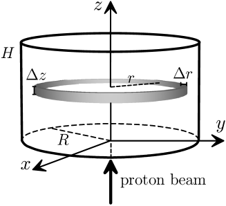
Figure 5: Schematics of the geometrical arrangement considered in the simulations.

We have run simulations of 50 million proton histories with these three models. The simulation speed (i.e., the number of simulated histories per CPU second) on an Intel i7 processor at 3.4 GHz was about 300 histories/s, nearly the same for the three models. Among other quantities, the program tallies the dose distribution $D(z,r)$ as a function of the depth $z$ and the radial distance $r$, using volume bins having the shape of a cylindrical ring with height $\Delta z=2$ mm and radial thickness $\Delta r=2$ mm. Because of the cylindrical symmetry of the arrangement, the efficiency of the simulation of the dose map is much higher than for unsymmetrical arrangements

Figure 6 displays the simulated depth-dose distributions $D(z)$, i.e., the energy deposited per unit mass thickness and per incident proton, as a function of depth within the water cylinder, calculated as

$$D(z)=\int_{0}^{R}D(z,r)\,2\pi r\,{\rm d}r.$$ (102)

The difference $D_{\rm pn}-D_{0}$ between the depth-doses calculated with the pn model and with the full physics measures the effect of the changes in the DCSs for elastic scattering that result from the finite size and the structure of nuclei. We see that replacing the “real” nucleus by a point nucleus causes a relatively small variation in the depth-dose only around the Bragg peak, which is shifted to slightly greater depths. This result indicates that oxygen atoms with point nuclei scatter less than atoms with real nuclei, in agreement with the fact that $F_{\rm nuc}$ is larger than unity at intermediate angles (see Fig. 2). The difference $D_{\rm pn-nor}-D_{0}$ between the depth-dose distributions obtained from the pn-nor model and the full model represents the global change in $D(z)$ caused by nuclear effects. Nuclear reactions have a strong impact on the depth-dose distributions, they produce a significant increase of $D(z)$ at shallow depths and an associated reduction of the primary proton flux that reaches the Bragg peak, with a corresponding reduction of the depth-dose distribution near that peak.

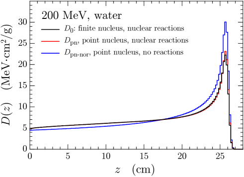
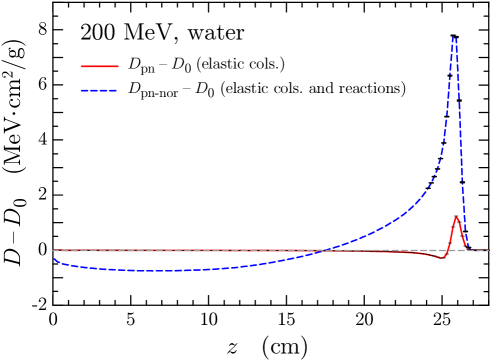
Figure 6: Top: Depth-dose distributions from a 200 MeV proton beam in water, calculated with the three physics models described in the text. Bottom: Depth-dose differences between simulations using the full model and the pn (point nucleus) and pn-nor (point nucleus, no nuclear reactions) models. Statistical uncertainties, shown as error bars in the bottom plot for $z>24$ cm, are generally less than the thicknesses of the curves.

The gammas and energetic light products released in nuclear reactions contribute to the dose at depths beyond the Bragg peak. Figure 7 displays the depth-dose curves in Fig. 6 with a logarithmic scale on the vertical axis to reveal the large-$z$ tail of $D(z)$. The pn-nor model produces a tail caused primarily by x rays, which extends to large depths. Nuclear reactions lead to an increase of the large-$z$ dose by two orders of magnitude, which is due to gammas and light reaction products. This increase in the dose may be relevant in the planning of protontherapy treatments of tumors located in front of sensitive organs.

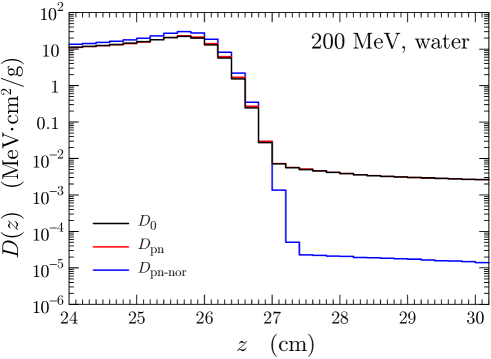
Figure 7: Depth-dose distributions from a 200 MeV proton beam in water in the Bragg peak zone and beyond, calculated with the three physics models described in the text.

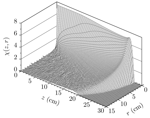
Figure 8: Three-dimensional plots of the dose function $\chi(z,r)=\log_{10}[1+D(z,r)]$, where $D(z,r)$ is the dose in units of eV/g, for a 200 MeV proton beam in water, calculated with the full physics model (top) and with the pn-nor model (bottom).

Nuclear effects also alter the radial distribution of dose, the changes become manifest when we compare dose maps obtained from the full physics and from the pn-nor model. Figure 8 shows three-dimensional plots of the function

$$\chi(z,r)=\log_{10}\left(1+D(z,r)\right),$$ (103)

with the dose $D(z,r)$ expressed in eV/g. Notice that $\chi\simeq D/\ln 10$ for small doses, and $\chi\simeq\log_{10}D$ when $D\gg 1$. That is, the plots display small doses on a nearly linear scale and large doses on a logarithmic scale. While the dose distribution calculated with the pn-nor model falls abruptly to nearly zero behind the Bragg peak and it decreases rapidly with the lateral distance $r$, the dose obtained from the full physics model decreases less rapidly with radial distance and it extends beyond the Bragg peak. The increase of the dose beyond the volume swept by the incident protons is caused by long-range energetic gammas and short-range light products emitted in proton-induced nuclear reactions.

6 Concluding comments

The program penh described in the present article differs from the 2013 version [28] in the consideration of nuclear effects in elastic collisions and in including proton-induced nuclear reactions. In addition, the description of elastic collisions has been reformulated by considering the correct relativistic equations of the motion of the colliding particles in the CM frame. Penh/penelope now provides a consistent description of electromagnetic and nuclear interactions in proton transport simulations. The accuracy of the simulation results is limited by the uncertainties of the adopted DCS models and of the description of nuclear reactions given by the available ENDF-6 files, the tracking of light products other than protons as “weighted equivalent” protons, and the neglect of the production and transport of neutrons released in nuclear reactions. Discrepancies with proton-beam dose measurements are to be expected at moderate and large lateral distances from the incident beam, which are mostly attributable to the neglected neutrons.

References

References

- [1] M. J. Berger, S. M. Seltzer, An overview of ETRAN Monte Carlo methods, in: T. M. Jenkins, W. R. Nelson, A. Rindi (Eds.), Monte Carlo Transport of Electrons and Photons, Plenum, New York, 1988, Ch. 7.
- [2] M. J. Berger, S. M. Seltzer, Applications of ETRAN Monte Cario codes, in: T. M. Jenkins, W. R. Nelson, A. Rindi (Eds.), Monte Carlo Transport of Electrons and Photons, Plenum, New York, 1988, Ch. 9.
- [3] M. J. Berger, S. M. Seltzer, ETRAN — Experimental Benchmarks, in: T. M. Jenkins, W. R. Nelson, A. Rindi (Eds.), Monte Carlo Transport of Electrons and Photons, Plenum, New York, 1988, Ch. 8.
- [4] J. A. Halbleib, R. P. Kensek, T. A. Mehlhorn, G. D. Valdez, S. M. Seltzer, M. J. Berger, ITS version 3.0: the integrated TIGER series of coupled electron/photon Monte Carlo transport codes, Tech. Rep. SAND91-1634, Sandia National Laboratories, Albuquerque, NM (1992).
- [5] W. R. Nelson, H. Hirayama, D. W. O. Rogers, The EGS4 Code System, Tech. Rep. SLAC-265, Stanford Linear Accelerator Center, Stanford, California (1985).
- [6] R. Brun, F. Bruyant, M. Maire, A. C. McPherson, P. Zanarini, GEANT3, Tech. Rep. DD/EE/84–1, CERN, Geneva (1987).
- [7] I. Kawrakow, D. W. O. Rogers, The EGSnrc code system: Monte Carlo simulation of electron and photon transport, Tech. Rep. PIRS-701, National Research Council of Canada, Ottawa (2001).
- [8] X-5 Monte Carlo Team, MCNP—A general Monte Carlo N-particle transport code, version 5, Report LA-UR-03-1987, Los Alamos National Laboratory, Los Alamos, NM, 2003.
- [9] S. Agostinelli, J. Allison, K. Amako, J. Apostolakis, H. Araujo, P. Arce, M. Asai, Geant4—a simulation toolkit, Nucl. Instrum. Meth. A 506 (2003) 250–303.
- [10] Allison, J., et al., Geant4 developments and applications, IEEE Trans. Nucl. Sci. 53 (2006) 270–278.
- [11] Allison, J., et al., Recent developments in Geant4, Nucl. Instrum. Meth. A 835 (2016) 186–225.
- [12] A. Ferrari, P. R. Sala, A. Fassò, J. Ranft, Fluka: a multi-particle transport code, Tech. Rep. CERN 2005 00X, INFN TC 05/11, SLAC R 773, CERN, Geneva (2005).
- [13] H. Hirayama, Y. Namito, A. F. Bielajew, S. J. Wilderman, W. R. Nelson, The EGS5 Code System, Tech. Rep. SLAC-R-730 (KEK 2005-8), Stanford Linear Accelerator Center, Menlo Park, California (2006).
- [14] J. T. Goorley, M. R. James, T. E. Booth, F. B. Brown, J. S. Bull, L. J. Cox, J. W. D. Jr., J. S. Elson, Initial MCNP6 Release Overview - MCNP6 version 1.0, LA-UR-13-22934, Los Alamos National Laboratory, Los Alamos, NM, 2013.
- [15] M. J. Berger, Monte Carlo calculation of the penetration and diffusion of fast charged particles, in: B. Alder, S. Fernbach, M. Rotenberg (Eds.), Methods in Computational Physics, Vol. 1, Academic Press, New York, 1963, pp. 135–215.
- [16] L. D. Landau, On the energy loss of fast particles by ionization, Journal of Physics-USSR 8 (1944) 201–205.
- [17] O. Blunck, S. Leisegang, Zum Energieverlust schneller Elektronen in dünnen Schichten, Z. Physik 128 (1950) 500–505.
- [18] H. Bichsel, R. P. Saxon, Comparison of calculational methods for straggling in thin absorbers, Phys. Rev. A 11 (1975) 1286–1296.
- [19] G. Molière, Theorie der Streuung schneller geladener Teilchen II: Mehrfach- und Vielfachstreuung, Z. Naturforsch. 3a (1948) 78–97.
- [20] S. Goudsmit, J. L. Saunderson, Multiple scattering of electrons, Phys. Rev. 57 (1940) 24–29.
- [21] S. Goudsmit, J. L. Saunderson, Multiple scattering of electrons. II, Phys. Rev. 58 (1940) 36–42.
- [22] H. W. Lewis, Multiple scattering in an infinite medium, Phys. Rev. 78 (1950) 526–529.
- [23] A. F. Bielajew, D. W. O. Rogers, PRESTA: The parameter reduced electron-step transport algorithm for electron Monte Carlo transport, Nucl. Instrum. Meth. B 18 (1987) 165–181.
- [24] B. Rossi, K. Greisen, Cosmic-ray theory, Rev. Mod. Phys. 13 (1941) 240–309.
- [25] L. Eyges, Multiple scattering with energy loss, Phys. Rev. 74 (1948) 1534–1535.
- [26] F. Salvat, penelope-2014: A code System for Monte Carlo Simulation of Electron and Photon Transport, OECD/NEA Data Bank, NEA/NSC/DOC(2015)3, Issy-les-Moulineaux, France, 2015, available from www.oecd-nea.org/science/docs/2015/nsc-doc2015-3.pdf.
- [27] J. Baró, J. Sempau, J. M. Fernández-Varea, F. Salvat, PENELOPE: An algorithm for Monte Carlo simulation of the penetration and energy loss of electrons and positrons in matter, Nucl. Instrum. Meth. B 100 (1995) 31–46.
- [28] F. Salvat, A generic algorithm for Monte Carlo simulation of proton transport, Nucl. Instrum. Meth. B 316 (2013) 144 –159.
- [29] A. Trkov, M. Herman, D. A. Brown, eds., ENDF-6 Formats Manual: Data Formats and Procedures for the Evaluated Nuclear Data Files, Tech. Rep. CSEWG Document ENDF-102. Report BNL-203218-2018-INRE SVN Commit: Rev. 215, Brookhaven National Laboratory, Upton, NY (2018).
- [30] F. Salvat, J. D. Martínez, R. Mayol, J. Parellada, Analytical Dirac-Hartree-Fock-Slater screening function for atoms ( = 1–92), Phys. Rev. A 36 (1987) 467–474.
- [31] G. Molière, Theorie der Streuung schneller geladener Teilchen I: Einzelstreuung am abgeschirmten Coulomb-Feld, Z. Naturforsch. 2a (1947) 133–145.
- [32] F. Salvat, J. M. Fernández-Varea, RADIAL: a Fortran subroutine package for the solution of the radial Schr dinger and Dirac wave equations, Comput. Phys. Commun. 240 (2019) 165–177.
- [33] F. D. Becchetti, G. W. Greenlees, Nucleon-nucleus optical-model parameters, , MeV, Phys. Rev. 182 (1969) 1190–1209.
- [34] P. E. Hodgson, The nuclear optical model, Rep. Prog. Phys. 34 (1971) 765–819.
- [35] A. Koning, J. Delaroche, Local and global nucleon optical models from 1 keV to 200 MeV, Nucl. Phys. A 713 (2003) 231–310.
- [36] J. D. Jackson, Classical Electrodynamics, 2nd Edition, John Wiley and Sons, New York, 1975.
- [37] H. Goldstein, Classical Mechanics, Addison-Wesley, Reading, MA, 1980.
- [38] A. Messiah, Quantum Mechanics, Dover Publications Inc., New York, 1999.
- [39] N. Bohr, The penetration of atomic particles through matter, K. Dan. Vidensk. Selsk. Mat. Fys. Medd. 18 (1948) 1–144.
- [40] L. I. Schiff, Quantum Mechanics, McGraw-Hill, Tokyo, 1968.
- [41] S. J. Wallace, Eikonal expansion, Phys. Rev. Lett. 27 (1971) 622–625.
- [42] M. Wang, G. Audi, A. Wapstra, F. Kondev, M. MacCormick, X. Xu, B. Pfeiffer, The Ame2012 atomic mass evaluation, Chinese Phys. C 36 (2012) 1603–2014.
- [43] E. Zeitler, H. Olsen, Complex scattering amplitudes in elastic electron scattering, Phys. Rev. 162 (1967) 1439–1447.
- [44] F. Olver, D. Lozier, R. Boisvert, C. Clark, NIST Handbook of Mathematical Functions, Cambridge University Press, New York, 2010, print companion to the NIST Digital Library of Mathematical Functions (DLMF), http://dlmf.nist.gov/.
- [45] G. D. Alkhazov, S. L. Belostotskij, A. A. Vorob’ev, Scattering of 1 GeV protons on 28Si, 32S, 34S nuclei, Yadernaya Fizika 22 (1975) 902–910.
- [46] M. Nakamura and H. Sakaguchi and H.Sakamoto and H. Ogawa and O. Cynshi and S. Kobayashi and S. Kato and N. Matsuoka and K. Hatanaka and T. Noro, Facility for the measurement of proton polarization in the range 50–70 MeV, Nucl. Instrum. Meth. 212 (1983) 173–184.
- [47] C. Olmer and A. D. Bacher and G. T. Emery and W. P. Jones and D. W. Miller and H. Nann and P. Schwandt and S. Yen and T. E. Drake and R. J. Sobie, Energy dependence of inelastic proton scattering to one-particle one-hole states in 28Si, Phys. Rev. C 29 (1984) 361–380.
- [48] K. H. Hicks and R. G. Jeppesen and C. C. K. Lin and R. Abegg and K. P. Jackson and O. Häusser and J. Lisantti and C. A. Miller and E. Rost and R. Sawafta and M. C. Vetterli and S. Yen, Inelastic proton scattering at 200 to 400 MeV for 24Mg and 28Si in a microscopic framework, Phys. Rev. C 38 (1988) 229–239.
- [49] E. García-Toraño, V. Peyres, F. Salvat, PenNuc: Monte Carlo simulation of the decay of radionuclides, Comput. Phys. Commun. 245 (2019) 106849.
- [50] D. Bote, F. Salvat, Calculations of inner-shell ionization by electron impact with the distorted-wave and plane-wave Born approximations, Phys. Rev. A 77 (2008) 042701.
- [51] C. C. Montanari, P. Dimitriou, The IAEA stopping power database, following the trends in stopping power of ions in matter, Nucl. Instrum. Meth. B 408 (2017) 50–55.
- [52] ICRU Report 49, Stopping Powers and Ranges for Protons and Alpha Particles, ICRU, Bethesda, MD, 1993.
- [53] M. J. Berger, ESTAR, PSTAR and ASTAR: computer programs for calculating stopping-power and range tables for electrons, protons and helium ions, Tech. Rep. NISTIR 4999, National Institute of Standards and Technology, Gaithersburg, MD, available from www.nist.gov/pml/data/star/index.cfm (1992).
- [54] A. Koning, D. Rochman, J. Sublet, N. Dzysiuk, M. Fleming, S. van der Marck, TENDL: Complete Nuclear Data Library for Innovative Nuclear Science and Technology, Nuclear Data Sheets 155 (2019) 1–55.
- [55] ICRU Report 63, Nuclear Data for Neutron and Proton Radiotherapy and for Radiation Protection, ICRU, Bethesda, MD, 2000.
- [56] C. Kalbach, Systematics of continuum angular distributions: Extensions to higher energies, Phys. Rev. C 37 (1988) 2350–2370.
- [57] A. J. Walker, An efficient method for generating discrete random variables with general distributions, ACM Trans. Math. Software 3 (1977) 253–256.
- [58] W. L. Dunn, J. K. Shultis, Exploring Monte Carlo Methods, Academic Press – Elsevier, Amsterdam, 2012.
- [59] J. Almansa, F. Salvat-Pujol, G. Díaz-Londoño, A. Carnicer, A. M. Lallena, F. Salvat, PENGEOM – A general-purpose geometry package for Monte Carlo simulation of radiation transport in complex material structures, Comput. Phys. Commun. 199 (2016) 102–113.