A Multi-Spatial, Multi-Temporal, Semi-Analytical Model for Bathymetry, Water Turbidity and Bottom Composition using Multispectral Imagery

Abstract

In this paper we introduce a semi-analytical model for bathymetry, water turbidity and bottom composition; which is primarily based on the physics-based model, HOPE, of Lee et al [14][15]. Unlike the model of Lee, which was originally designed to use hyperspectral imagery, our model is specifically designed to use multispectral satellite imagery. In particular, we adapt to the greatly decreased spectral resolution by introducing temporal and spatial assumptions on the depth and water turbidity. We validate the extensions to the Lee et al model with a 260 $\text{km}^{2}$ case study in the area of the Murion Islands off Western Australia, where we compare the atmospherically-corrected LANDSAT-8 derived bathymetry against a 2011 single-beam sonar survey by Transport Western Australia. The model validates well against the single-beam sonar survey, with $R^{2}=0.77$, a mean absolute error of 1.37 m and a mean relative error of 9.24%. This indicates the model could be widely applicable to LANDSAT-8 imagery.

Keywords: Remote sensing, satellite-derived bathymetry, multispectral imagery, radiative transfer models, LANDSAT-8.

Table 1: Symbols

symbol	description	units
$R_{\text{rs}}$	remote sensing reflectance (RRS)	$\text{sr}^{-1}$
$r_{\text{rs}}$	subsurface remote sensing reflectance	$\text{sr}^{-1}$
$P$	phytoplankton absorption coefficient at 440 nm	$\text{m}^{-1}$
$G$	absorption coefficient of gelbstoff and detritus at 440 nm	$\text{m}^{-1}$
$X$	backscattering coefficient of particles at 440 nm	$\text{m}^{-1}$
$B$	bottom albedo at 550 nm
$H$	bottom depth	m
$\Delta$	spectrally-constant offset	$\text{sr}^{-1}$
$a$	absorption coefficient	$\text{m}^{-1}$
$b_{b}$	backscattering coefficient	$\text{m}^{-1}$
$k$	attenuation coefficient	$\text{m}^{-1}$
$\rho$	bottom albedo spectrum normalised to 550 nm
$\theta_{\text{sun}}$	subsurface solar zenith angle	rad
$\theta_{\text{view}}$	subsurface viewing angle from nadir	rad

1 Introduction

The origins of marine remote sensing by satellite date to the early 1970s with the launch of LANDSAT 1 and the seminal research of Polcyn & Cousteau [1][4]. In 1975, NASA and Jacques Cousteau used multispectral imagery from LANDSAT 1 and in situ measurements of water clarity and sea floor reflectance to estimate the bathymetry in the Bahamas and off the eastern coast of Florida. They concluded that with optimal conditions, satellite-derived depths could be reliably modelled up to a depth of 22 m. Polcyn initially used a single band to estimate the depth, where the band attenuation coefficient and bottom reflectance was measured at the same time as the satellite image acquisition. Later Polcyn generalised this method to a depth estimate based on the ratio of two bands. As the field measurements were taken at a single location, these depth estimates assumed constant water turbidity and bottom reflectance across the entire satellite scene.

In 1978, Lyzenga [6] introduced an empirical multi-band method to estimate the bathymetry. Like the ratio method of Polcyn, this method assumed constant water turbidity and bottom type. The Lyzenga method is outlined in Section 4.1. In 2006, Lyzenga et al refined this method [24].

Since the turn of the century, physics-based radiative transfer models have existed to simultaneously estimate depth, water turbidity and bottom reflectance from hyperspectral imagery. A detailed summary and inter-comparison at two sites of a number of key models is given in Dekker et al [33].

The original model of Lee et al [14][15], HOPE (Hyperspectral Optimisation Process Exemplar), assumed a single benthic substratum (sand). Lee et al [16] subsequently generalised this to two benthic substratum - sand and seagrass, where the two were delineated by way of an empirical relationship prior to the model inversion. The HOPE model originally used the SOLVER tool (within Microsoft Excel) as the optimisation routine. Subsequently, HOPE used the Levenberg-Marquardt and B2NLS optimisation algorithms [27].

In 2004, Klonowski et al [20][26] made extensions to the model of Lee et al to classify bottom spectra in Jurien Bay, Western Australia. Modifications were made to the model of Chlorophyll-a concentrations, based on measurements in Cockburn Sound. This model included a parameterisation for three bottom spectra - sand, Hallophylla (green leafy seagrass) and Sargassum (brown seaweed). This model used the Levenburg-Marquardt optimisation scheme.

In 2005, Mobley et al [23] used the radiative transfer numerical model, HydroLight, to construct lookup tables for spectrum matching of hyperspectral imagery. This model is known as CRISTAL (Comprehensive Reflectance Inversion based on Spectrum matching and TAble Lookup) [33].

In 2006, Wettle et al [25][29] developed a semi-analytical model, SAMBUCA (Semi-Analytical Model for Bathymetry, Un-mixing, and Concentration Assessment), based on the Lee et al model, HOPE. This model incorporates a different parameterisation for the absorption and backscatter coefficients to HOPE, which is in line with field data measurement protocols used by the CSIRO. This model used the Simplex optimisation scheme.

In 2009, Hedley et al [28] implemented an efficient lookup table inversion scheme for radiative transfer models using adaptive lookup trees (ALUT). This model was more efficient than optimisation-based models and had comparable accuracy in bathymetric retrievals.

In 2014, Gege [19] used the shallow water parameterisation of the RRS by Albert and Mobley [18] to implement the WASI (Water Colour Simulator) model. This parameterisation is an alternative to the model of Lee et al. This model uses the simplex optimisation scheme.

In 2018, Hedley et al [35] examined the use of the Sentinel-2 satellite to monitor coral reefs. It was found that the Sentinel-2 data can be used within a physics-based model to monitor coral reefs and retrieve bathymetric estimations with comparable performance to WorldView-2.

In this paper we detail the development of the photic model, an extension of the Lee et al [14][15][16] semi-analytical model for use with multispectral imagery. In particular, for the LANDSAT-8 and Sentinel-2 satellites. These satellites have greatly decreased spectral resolution in comparison to airborne hyperspectral sensors, however they have regular global coverage in coastal areas and their datasets are freely available. Given this availability, we are motivated to see if we can apply semi-analytical models accurately and efficiently to these datasets.

In section 2 we recap the hyperspectral model of Lee et al [14][15][16], along with extensions to include multiple bottom types by Gege [19] and Wettle et al [25]. We follow Wettle et al [25] and use both the root-mean-square and spectral angle mapper error in our error metric.

In section 3 we introduce spatial and temporal extensions to the Lee et al model.

In section 4 we detail how the model is inverted to yield stable depth, water turbidity and bottom reflectance estimates.

In section 5 we detail an iterative modelling framework, where model parameters are estimated and subsequently refined to improve their retrieval.

In section 6 we give a detailed case study where we validate the photic model against single-beam sonar data in the area of the Murion Island Marine Management Area.

2 The Model for Hyperspectral Imagery

Our modelling approach for hyperspectral imagery directly follows the model of Lee et al [14][15][16], with additions to include multiple bottom spectra as given in the model of Gege [19] and the spectral angle mapper (SAM) in the spectral matching error metric as given in the model of Wettel et al [25]. We will now briefly describe the model.

The remote-sensing reflectance (RRS), $R_{rs}$, is defined at the ratio of the water leaving radiance to downwelling irradiance just above the surface. The RRS over optically shallow water is controlled by a number of factors, including absorption properties, scattering properties, the bottom albedo, bottom depth and solar elevation. We begin by relating the RRS above the surface, $R_{rs}(\lambda)$, to the subsurface RRS, $r_{rs}(\lambda)$ which is given by

$$R_{rs}(\lambda)=\frac{0.5\,r_{rs}(\lambda)}{1-1.5\,r_{rs}(\lambda)}+\Delta,$$

where $\Delta$ is a spectrally-constant offset. The subsurface RRS, $r_{rs}(\lambda)$, is expressed as a linear combination of subsurface RRS from the water column, $r_{rs_{C}}(\lambda)$, and the subsurface RRS from the bottom reflectance, $r_{rs_{B}(\lambda)}$.

$$r_{rs}(\lambda) =r_{rs_{C}}(\lambda)+r_{rs_{B}}(\lambda)$$

$$=r_{rs_{\infty}}(\lambda)\left(1-\exp\left(-\left(\frac{1}{\cos(\theta_{\text{sun}})}+\frac{D_{C}(\lambda)}{\cos(\theta_{\text{view}})}\right)\,k(\lambda)\,H\right)\right)+$$

$$\qquad\frac{\rho(\lambda)}{\pi}\exp\left(-\left(\frac{1}{\cos(\theta_{\text{sun}})}+\frac{D_{B}(\lambda)}{\cos(\theta_{\text{view}})}\right)\,k(\lambda)\,H\right)$$ (2.1)

Where $r_{rs_{\infty}}(\lambda)$ is the subsurface RRS for optically deep water. $D_{C}(\lambda)$ and $D_{B}(\lambda)$ are the path elongation for photons from the water column and from the bottom respectively. $\theta_{\text{sun}}$ is the subsurface solar zenith angle and $\theta_{\text{view}}$ is the subsurface viewing angle from nadir. $\rho(\lambda)$ is the bottom albedo. $H$ is the bottom depth. $k(\lambda)$ is the attenuation coefficient, which is given by

$$k(\lambda)=a(\lambda)+b_{b}(\lambda)$$ (2.2)

where $a(\lambda)$ is the absorption coefficient and $b_{b}(\lambda)$ is the backscattering coefficient.

For the subsurface RRS of optically deep water, Lee et al [14][15][16] used the model of Gordon et al [8]

$$r_{\infty}(\lambda)=0.084\,u(\lambda)+0.170\,u(\lambda)^{2},$$

where

$$u(\lambda)=\frac{b_{b}(\lambda)}{a(\lambda)+b_{b}(\lambda)}.$$

The path elongation factors are given by

$$D_{C}(\lambda) =1.03\sqrt{1+2.4u}$$

$$D_{B}(\lambda) =1.04\sqrt{1+5.4u}.$$

The inherent optical properties, $a(\lambda)$ & $b_{b}(\lambda)$ are given by

$$a(\lambda)=a_{w}(\lambda)+a_{\phi}(\lambda)+a_{g}(\lambda)$$

$$b(\lambda)=b_{bw}(\lambda)+b_{bp}(\lambda),$$

where $a_{w}(\lambda)$ is the absorption coefficients of pure water as given in Pope & Fry [12], $a_{\phi}(\lambda)$ is the absorption coefficients for phytoplankton pigments, $a_{g}(\lambda)$ is the absorption coefficients for gelbstoff and detrius, $b_{bw}(\lambda)$ is the backscattering coefficient for pure seawater as given in Morel [3], $b_{bp}(\lambda)$ is the backscattering coefficient of suspended particles.

For an $n$-band spectrum the model above has $n$ equations (one for each $\lambda$), each with 4 unknowns – $a_{\phi}(\lambda),a_{g}(\lambda),b_{bp}(\lambda),\rho(\lambda),H$. Thus, there are $4n+1$ unknowns and $n$ equations, and consequently finding solutions to this system requires establishing additional relationships.

Lee et al estimated the spectral shape of $a_{\phi}(\lambda)$ with a single parameter, $P$, which represents the phytoplankton absorption coefficient at 440 nm, ie. $P=a_{\phi}(440)$

$$a_{\phi}(P,\lambda)=\left(a_{0}(\lambda)+a_{1}(\lambda)\log(P)\right)P,$$ (2.3)

where $a_{0}(\lambda)$, $a_{1}(\lambda)$ was modelled by Lee [10]. We use this model for $a_{\phi}$, however we derived the parameterisation of $a_{0}(\lambda)$, $a_{1}(\lambda)$ from a dataset sourced from the CSIRO [21] (See Appendix A).

The spectral shape for the absorption of gelbstoff and detritus, $a_{g}(\lambda)$ is expressed with the parameter $G=a_{g}(440)$ and is given by

$$a_{g}(G,\lambda)=G\,e^{-S(\lambda-440)}.$$

The parameter S is in the range $0.011$–$0.021$ $\text{nm}^{-1}$.

The spectral shape for the backscattering coefficient of suspended particles, $b_{bp}(\lambda)$ is expressed with the parameter $X=b_{bp}(440)$ and is given by

$$b_{bp}(X,\lambda)=X\,\left(\frac{440}{\lambda}\right)^{Y},$$

where $Y$ is estimated by the empirical relationship

$$Y=3.44\left(1.0-3.17e^{-2.01\chi}\right)\quad\text{and}\quad\chi=\frac{R_{rs}(440)-R_{rs}(750)}{R_{rs}(490)-R_{rs}(750)}.$$

Finally, for $N_{b}$ bottom types, the bottom albedo is parameterised with $B=\rho(550)$ and we write $\rho(\lambda)$ as $\rho(B,q_{0},q_{1},\cdots,q_{N_{b}-1},\lambda)$, where

$$\rho(B_{0},B_{1},\cdots,B_{N_{b}-1},q_{0},q_{1},\cdots,q_{N_{b}-1},\lambda)=\frac{\sum\limits_{i=0}^{N_{b}-1}B_{i}\,q_{i}\,\rho_{\text{bottom}_{i}}(\lambda)}{\sum\limits_{i=0}^{N_{b}-1}q_{i}},$$ (2.4)

where $\rho_{\text{bottom}_{i}}(\lambda)$ is the bottom albedo of a given bottom type as estimated from field measurements and normalised to 550 nm, and the $q_{i}$ specify the fraction of each bottom type. This is based on the parameterisations used in Gege [19] and Wettle et al [25].

Our model can estimate bottom reflectance using (2.4), however if the model is required to delineate between a large number of bottom spectra then we are better to adopt the iterative method of Wettle et al [25]. In this formulation, we iterate over all individual bottom spectra, then over all pairs of bottom spectra. The spectra or pair of spectra best matching the input RRS is then representative of the bottom composition. It is worth noting that this method is significantly slower due to the combinatorial nature of exhaustively iterating through all the pairs.

With this parameterisation we reduce the number of unknowns which influence the RRS spectrum to $P$, $G$, $X$, $B_{0}$, $B_{1}$, $\cdots$, $B_{N_{b}-1}$, $q_{0},q_{1},\cdots,q_{N_{b}-1}$, $H$ and $\Delta$. Thus if we have $5+2N_{b}$ independent channels it should be possible to determine a unique solution to the system of equations. However due to the presence of noise the best we can do is seek to minimise the difference between the modelled RRS, $R_{rs_{\text{modelled}}}(\lambda)$, and the measured RRS, $R_{rs_{\text{measured}}}(\lambda)$. Following Lee et al [14][15][16], we define the RRS RMS relative error, $E_{R_{rs}}^{\text{RMS}}$, as

$$E_{R_{rs}}^{\text{RMS}}(P,G,X,B_{0},B_{1},\cdots,B_{N_{b}-1},q_{0},q_{1},\cdots,q_{N_{b}-1},H,\Delta)=\\ \frac{\sqrt{\sum\limits_{\lambda}\left(R_{rs_{\text{modelled}}}(\lambda)-R_{rs_{\text{measured}}}(\lambda)\right)^{2}}}{\sum\limits_{\lambda}R_{rs_{\text{measured}}}(\lambda)}.$$ (2.5)

Wettle et al [25] included the Spectral Angle Mapper (SAM) within the error metric

$$E_{R_{rs}}^{\text{SAM}}(P,G,X,B_{0},B_{1},\cdots,B_{N_{b}-1},q_{0},q_{1},\cdots,q_{N_{b}-1},H,\Delta)=\\ \cos^{-1}\left(\frac{R_{rs_{\text{modelled}}}\cdot R_{rs_{\text{measured}}}}{\left(R_{rs_{\text{modelled}}}\cdot R_{rs_{\text{modelled}}}\right)\left(R_{rs_{\text{measured}}}\cdot R_{rs_{\text{measured}}}\right)}\right),$$

where in both $E_{R_{rs}}^{\text{RMS}}$ and $E_{R_{rs}}^{\text{SAM}}$ the term $R_{rs_{\text{modelled}}}$ is dependent on the parameters $P$, $G$, $X$, $B_{0}$, $B_{1}$, $\cdots$, $B_{N_{b}-1}$, $q_{0}$, $q_{1}$, $\cdots$, $q_{N_{b}-1}$, $H$, $\Delta$ and $\lambda$. We will describe the full error metric used in photic in the following section.

3 Extensions to the Model for Multispectral Imagery

Lee et al [17] found that 15 equispaced spectral bands covering the 400–800 nm range are adequate for most coastal and oceanic remote sensing applications. The satellite imagery of LANDSAT 8 and Sentinel-2 have significantly fewer spectral bands in this range, however we would still like to apply the semi-analytical model to these vast and freely available datasets. Previously Dekker et al [34] has applied the SAMBUCA [25] model to QuickBird multispectral satellite imagery.

We now describe two extensions to the semi-analytical model to increase its applicability to multispectral imagery.

3.1 Spatial extension

A reasonable assumption to make for medium to high resolution satellite imagery is constant water turbidity within a spatial region around a given pixel. Klonowski et al [20] used a constant $P$, $G$ and $X$ throughout an entire scene for bottom type classification using hyperspectral imagery.

If we define a spatial region, $r$, around a given pixel, then we (simultaneously) model $N_{r}=(2r+1)^{2}$ pixels. Within this region we constrain $P$, $G$, $X$ and $\Delta$ to be (spatially) static, while $H$, $B_{0}$, $B_{1}$, $\cdots$, $B_{N_{b}-1}$, $q_{0}$, $q_{1}$, $\cdots$, $q_{N_{b}-1}$ may vary.

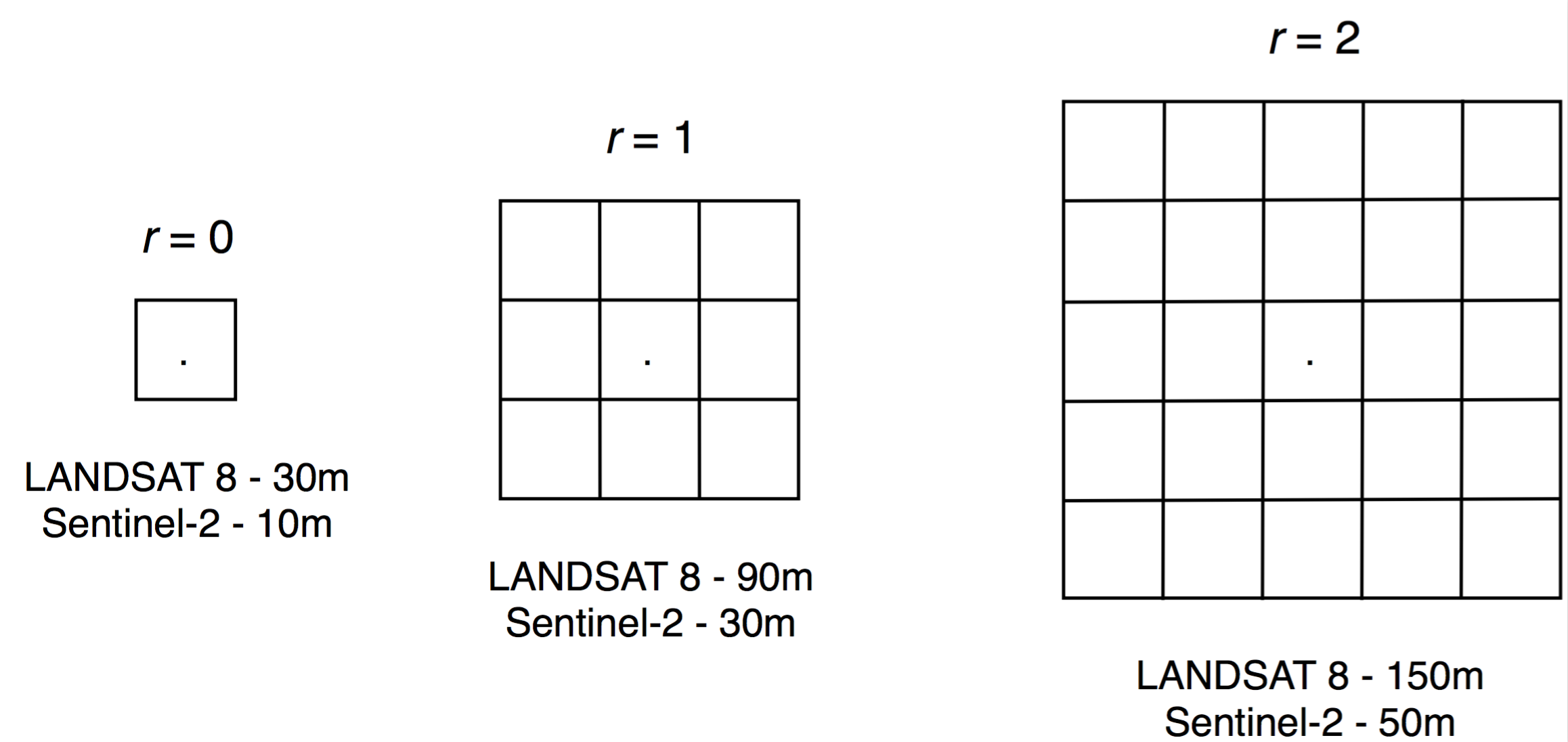
Figure 1: The spatial grid around the modelled pixel for different $r$.

Thus, we may represent the non-static parameters within each region as

$$\begin{split}\textbf{H}&=\left[H_{0},H_{1},\cdots,H_{N_{r}-1}\right]\\ \textbf{B}_{0}&=\left[B_{0,0},B_{0,1},\cdots,B_{0,N_{r}-1}\right]\\ \textbf{B}_{1}&=\left[B_{1,0},B_{1,1},\cdots,B_{1,N_{r}-1}\right]\\ &\vdots\\ \textbf{B}_{N_{b}-1}&=\left[B_{N_{b}-1,0},B_{N_{b}-1,1},\cdots,B_{N_{b}-1,N_{r}-1}\right]\\ \textbf{q}_{0}&=\left[q_{0,0},q_{0,1},\cdots,q_{0,N_{r}-1}\right]\\ \textbf{q}_{1}&=\left[q_{1,0},q_{1,1},\cdots,q_{1,N_{r}-1}\right]\\ &\vdots\\ \textbf{q}_{N_{b}-1}&=\left[q_{N_{b}-1,0},q_{N_{b}-1,1},\cdots,q_{N_{b}-1,N_{r}-1}\right]\\ \end{split}$$ (3.1)

Additionally, in many instances it is reasonable to constrain the variance of H within the spatial region. That is, a constraint of the form $\sigma\left(\textbf{H}\right)<\kappa\,\mkern 1.5mu\overline{\mkern-1.5mu\textbf{H}\mkern-1.5mu}\mkern 1.5mu,$ with $\kappa=0.1$. Where $\sigma\left(\textbf{H}\right)$ and $\mkern 1.5mu\overline{\mkern-1.5mu\textbf{H}\mkern-1.5mu}\mkern 1.5mu$ is the standard deviation and mean of H respectively. (Alternatively, $\kappa$ can be dependent on depth.) The error metric we use in photic for the continuity of H is given by

$$E_{\textbf{H}}=\sqrt{\frac{1}{N_{r}}\sum\limits_{i=0}^{N_{r}-1}\begin{cases}\left(\frac{H_{i}-\mkern 1.5mu\overline{\mkern-1.5mu\textbf{H}\mkern-1.5mu}\mkern 1.5mu}{\mkern 1.5mu\overline{\mkern-1.5mu\textbf{H}\mkern-1.5mu}\mkern 1.5mu}\right)^{2}&\left|H_{i}-\mkern 1.5mu\overline{\mkern-1.5mu\textbf{H}\mkern-1.5mu}\mkern 1.5mu\right|>\kappa\,\mkern 1.5mu\overline{\mkern-1.5mu\textbf{H}\mkern-1.5mu}\\ 0&\text{otherwise}\end{cases}}.$$ (3.2)

3.2 Temporal extension

We can further increase the spectral data available to the model by using a time series of satellite scenes. For LANDSAT-8 and Sentinel-2 scenes, a large number of scenes are available and most are usable for our purposes.

We assume continuity of the seabed over time. Thus, across multiple scenes the depth, $H$, is static up to tidal effects. For $N_{s}$ scenes, it is assumed we know the tidal corrections $H_{\text{tide}_{0}}$, $H_{\text{tide}_{1}}$, $\cdots$, $H_{\text{tide}_{N_{s}-1}}$ to a common datum, such that

$$H+H_{\text{tide}_{0}}=H+H_{\text{tide}_{1}}=\cdots=H+H_{\text{tide}_{N_{s}-1}}.$$

We further assume the bottom reflectance is constant over time. This may be a more tenuous assumption than our other assumptions, for example for some coral reefs or seagrass beds.

Thus, the temporal constraints are $H$, $B_{0}$, $B_{1}$, $\cdots$, $B_{N_{b}-1}$, $q_{0}$, $q_{1}$, $\cdots$ and $q_{N_{b}-1}$ are constant, while allowing the water turbidity to vary over time - $P$, $G$, $X$ (and $\Delta$), which we represent as

$$\begin{split}\textbf{P}&=\left[P_{0},P_{1},\cdots,P_{N_{s}-1}\right]\\ \textbf{G}&=\left[G_{0},G_{1},\cdots,G_{N_{s}-1}\right]\\ \textbf{X}&=\left[X_{0},X_{1},\cdots,X_{N_{s}-1}\right]\\ \mathbf{\Delta}&=\left[\Delta_{0},\Delta_{1},\cdots,\Delta_{N_{s}-1}\right].\end{split}$$ (3.3)

These constraints complement the spatial constraints, in that previously $H$, $B_{0}$, $B_{1}$, $\cdots$, $B_{N_{b}-1}$, $q_{0}$, $q_{1}$, $\cdots$, $q_{N_{b}-1}$ could vary spatially, while $P$, $G$, $X$ are spatially static.

3.3 The multi-spatial, multi-temporal, error metric

We will now combine the spatial and temporal extensions into a single error metric for our model. As before, let $N_{s}$ be the number of satellite scenes and $N_{r}$ the size of the spatial region around the spectra we are modelling. Then denote $R_{rs_{{\text{measured}}_{i}}}^{j}(\lambda)$ and $R_{rs_{{\text{modelled}}_{i}}}^{j}(\lambda)$ to be the measured and modelled RRS at spatial location $i$ (for $i=0,\cdots,N_{r}-1$) and scene $j$ (for $j=0,\cdots,N_{s}-1$) for wavelength, $\lambda$, respectively. Then the RMS error across all scenes and the entire region is given by

$$E_{R_{rs}}^{\text{RMS}}\left(\textbf{P},\textbf{G},\textbf{X},\textbf{B}_{0},\textbf{B}_{1},\cdots,\textbf{B}_{N_{b}-1},\textbf{q}_{0},\textbf{q}_{1},\cdots,\textbf{q}_{N_{b}-1},\textbf{H},\mathbf{\Delta}\right)=\\ \frac{\sqrt{\sum\limits_{i=0}^{N_{r}-1}\sum\limits_{j=0}^{N_{s}-1}\sum\limits_{\lambda}\left(R_{rs_{{\text{modelled}}_{i}}}^{j}(\lambda)-R_{rs_{{\text{measured}}_{i}}}^{j}(\lambda)\right)^{2}}}{\sum\limits_{i=0}^{N_{r}-1}\sum\limits_{j=0}^{N_{s}-1}\sum\limits_{\lambda}R_{rs_{{\text{measured}}_{i}}}^{j}(\lambda)},$$ (3.4)

similarly, the SAM error is given by

$$E_{R_{rs}}^{\text{SAM}}\left(\textbf{P},\textbf{G},\textbf{X},\textbf{B}_{0},\textbf{B}_{1},\cdots,\textbf{B}_{N_{b}-1},\textbf{q}_{0},\textbf{q}_{1},\cdots,\textbf{q}_{N_{b}-1},\textbf{H},\mathbf{\Delta}\right)=\\ \frac{1}{N_{r}N_{s}}\sum\limits_{i=0}^{N_{r}-1}\sum\limits_{j=0}^{N_{s}-1}\cos^{-1}\left(\frac{R_{rs_{{\text{modelled}}_{i}}}^{j}\cdot R_{rs_{{\text{measured}}_{i}}}^{j}}{\left(R_{rs_{{\text{modelled}}_{i}}}^{j}\cdot R_{rs_{{\text{modelled}}_{i}}}^{j}\right)\left(R_{rs_{{\text{measured}}_{i}}}^{j}\cdot R_{rs_{{\text{measured}}_{i}}}^{j}\right)}\right),$$ (3.5)

where H, $\textbf{B}_{0}$, $\textbf{B}_{1}$, $\cdots$, $\textbf{B}_{N_{b}-1}$, $\textbf{q}_{0}$, $\textbf{q}_{1}$, $\cdots$, $\textbf{q}_{N_{b}-1}$ are given in (3.1), and P, G, X, $\mathbf{\Delta}$ are given in (3.3). We denote $R_{rs_{{\text{modelled}}_{i}}}^{j}(\lambda)$ as shorthand for $R_{rs_{{\text{modelled}}_{i}}}^{j}(\textbf{P},$ $\textbf{G},$ $\textbf{X},$ $\textbf{B}_{0},$ $\textbf{B}_{1},$ $\cdots,$ $\textbf{B}_{N_{b}-1},$ $\textbf{q}_{0},$ $\textbf{q}_{1},$ $\cdots,$ $\textbf{q}_{N_{b}-1},$ $\textbf{H},$ $\mathbf{\Delta},$ $\lambda)$.

We have three error metrics - the RMS error (3.4), the SAM error (3.5), and the continuity of H error (3.2). We combine these into a final, weighted, error metric for our model,

$$E_{\text{photic}}=\omega_{0}\,E_{R_{rs}}^{\text{RMS}}E_{R_{rs}}^{\text{SAM}}+\omega_{1}\,E_{H},$$ (3.6)

where $\omega_{0}\gg\omega_{1}$ and $\omega_{0}+\omega_{1}=1$. In photic, we experimentally found $\omega_{0}=0.85$ and $\omega_{1}=0.15$ balances both terms in the error metric.

In this formulation of the model, we have $N_{r}$ parameters for H; $N_{b}\,N_{r}$ parameters for $\textbf{B}_{0}$, $\textbf{B}_{1}$, $\cdots$, $\textbf{B}_{N_{b}-1}$; $N_{b}\,N_{r}$ parameters for $\textbf{q}_{0}$, $\textbf{q}_{1}$, $\cdots$, $\textbf{q}_{N_{b}-1}$; and $4N_{s}$ parameters for P, G, X, $\mathbf{\Delta}$. In total, we have

$$N_{\text{total}}=N_{r}+2\,N_{b}\,N_{r}+4N_{s}$$

parameters to determine.

These spatial and temporal extensions to the model of Lee et al greatly increase data used in the spectral matching. Below we compare the number of measured spectra (assuming we use the LANDSAT 8 satellite with the coastal, blue, green and red spectral bands) across each scene and region to the number of unknown parameters in our model, where the number of bottom types, $N_{b}$ is 2.

Table 2: In the table on the left we list the number of (simultaneous) equations for the LANDSAT 8 satellite; and in the table on the right we list the number of model unknowns. Both of these are a function of the number of satellite scenes ($N_{s}$), the region size ($N_{r}$), and the number of bottom types ($N_{b}$), which for this table $N_{b}=2$.

$\begin{array}[]{cc|ccc}&\lx@intercol\hfil\hfil\lx@intercol&\lx@intercol\hfil N_{r}\hfil\lx@intercol\\ &N_{\text{landsat 8}}&1&9&25\\ \cline{2-5}\cr&1&4&36&100\\ \smash{\rotatebox[origin={c}]{90.0}{$N_{s}$}}&2&8&\textbf{72}&200\\ &3&12&108&300\\ &4&16&144&400\end{array}$   $\begin{array}[]{cc|ccc}&\lx@intercol\hfil\hfil\lx@intercol&\lx@intercol\hfil N_{r}\hfil\lx@intercol\\ &N_{\text{total}}&1&9&25\\ \cline{2-5}\cr&1&9&49&129\\ \smash{\rotatebox[origin={c}]{90.0}{$N_{s}$}}&2&13&\textbf{53}&133\\ &3&17&57&137\\ &4&21&61&141\end{array}$

A common setting for our modelling is $N_{s}=2$, $N_{r}=9$ and $N_{b}=2$, which is highlighted above.

4 Inverting the Model

We will now detail how we invert (2.1) to obtain estimates for P, G, X, $\textbf{B}_{0}$, $\textbf{B}_{1}$, $\cdots$, $\textbf{B}_{N_{b}-1}$, H, $\textbf{q}_{0}$, $\textbf{q}_{1}$, $\cdots$, $\textbf{q}_{N_{b}-1}$ and $\mathbf{\Delta}$ by finding a (global) minimum of $E_{\text{photic}}$.

4.1 Initial depth estimate

Lee et al [15] used $H=10.0$ m as an initial depth estimate and subsequently used an estimate of $H=1/(6P)$ [33]. Starting the model inversion at a reasonable depth estimate was a technique used by Albert et al [22].

If reliable depth profiles are known, then initial, and often accurate, depth estimates can be obtained using an empirical method [4][6][24]. Closely following the model of Lyzenga et al [24] - the empirical depth, $H_{\text{empirical}}$, for a $n$-band spectrum is given by

$$H_{\text{empirical}}\left(h_{1},h_{2},\cdots,h_{n}\right)=h_{0}-\sum_{i=1}^{n}h_{i}\log(r_{rs}(\lambda_{i-1})-r_{rs_{\infty}}(\lambda_{i-1})),$$

where $h_{0}=\sum\limits_{i=1}^{n}h_{i}\log(\rho(\lambda_{i-1})/\pi)$ and $\sum\limits_{i=1}^{n}h_{i}\,k(\lambda_{i-1})=1$.

The subsurface RRS of optically deep waters is estimated using the method of Lyzenga et al [24]. We compute both the mean subsurface RRS of optically deep water, $\mkern 1.5mu\overline{\mkern-1.5mur\mkern-1.5mu}\mkern 1.5mu_{rs_{\infty}}(\lambda)$, and the standard deviation of the subsurface RRS of optically deep water, $\sigma\left(r_{rs_{\infty}}(\lambda)\right)$ in each band. It is worth noting that this is a scene-wide estimate.

The attenuation coefficients are estimated using the blue and green spectral bands

$$\frac{k(\text{blue})}{k(\text{green})}\approx\frac{\log\left(r_{rs}(\text{blue})-r_{rs_{\infty}}(\text{blue})\right)}{\log\left(r_{rs}(\text{green})-r_{rs_{\infty}}(\text{green})\right)},$$

then interpolate across spectra and water types from a table of spectral attenuation coefficients for different coastal and oceanic water types to directly estimate the attenuation coefficients and the water type [5][13]. Again, it is worth noting that this is a scene-wide estimate.

Consider $N$ soundings $s_{0},s_{1},\cdots,s_{N-1}$, we begin by generating weights for each soundings $w_{0},w_{1},\cdots,w_{N-1}$ such that

$$w_{i}=1-W_{i}/M,\quad\text{where}\quad W_{i}=\sum\limits_{j=0}^{N-1}e^{-\left(s_{i}-s_{j}\right)^{2}},$$

where $M=\max(W_{0},W_{1},\cdots,W_{N-1})$. This weighting scheme prevents frequently occurring depths from skewing the subsequence fitting. We construct a weighted, root-mean-square, relative error metric, $E_{\text{empirical}}$, such that

$$E_{\text{empirical}}\left(h_{1},h_{2},\cdots,h_{n}\right)=\sqrt{\frac{\sum\limits_{i=0}^{N-1}w_{i}\left(\frac{H_{\text{empirical}_{i}}-s_{i}}{s_{i}}\right)^{2}}{\sum\limits_{i=0}^{N-1}w_{i}}},$$

where $H_{\text{empirical}_{i}}$ is shorthand for $H_{\text{empirical}_{i}}\left(h_{1},h_{2},\cdots,h_{n}\right)$ at the spatial location of the sounding, $s_{i}$.

To find the minima of $E_{\text{empirical}}$, we use multiple iterations of the simplex algorithm [2], each with a pseudo-randomly generated initial simplex. This random initialisation with multiple iterations helps prevent the optimisation from settling in a local minimum.

With multiple scenes, the depths from each scene from the empirical algorithm can be synthesised into a single depth estimate by way of a temporal median across all modelled scenes (once we account for tidal variations). Alternatively, a weighted mean can be used. In this case, the weights are inversely proportional to the final $E_{\text{empirical}}$ of each scene.

4.2 Ordering pixels by spectral angle

It would be natural within a computer implementation to model the pixels in a column- or row-major order. However in photic, pixels within the modelling domain are sorted by spectral angle above the deep water mean (via the SAM). The spatial indices of the pixels are stored so we can return the modelling results to their original location. The model starts with the pixels closest to the mean deep water spectrum. We will subsequently see why this ordering is favourable to our modelling.

4.3 Initial estimates for P, G, X and $\mathbf{\Delta}$

The initial estimates closely follows Lee et al [15]. Without any knowledge of field samples, the initial parameterisation of P, G, X and $\mathbf{\Delta}$ is given by

$$P_{j} =0.072\left({\mkern 1.5mu\overline{\mkern-1.5muR\mkern-1.5mu}\mkern 1.5mu_{rs}}^{j}(440)/{\mkern 1.5mu\overline{\mkern-1.5muR\mkern-1.5mu}\mkern 1.5mu_{rs}}^{j}(550)\right)^{-1.7}$$

$$G_{j} =1.5P_{j}$$

$$X_{j} =30\,a_{w}(640){\mkern 1.5mu\overline{\mkern-1.5muR\mkern-1.5mu}\mkern 1.5mu_{rs}}^{j}(640)$$

$$\Delta_{j} ={\mkern 1.5mu\overline{\mkern-1.5muR\mkern-1.5mu}\mkern 1.5mu_{rs}}^{j}(750)$$

where $\mkern 1.5mu\overline{\mkern-1.5muR\mkern-1.5mu}\mkern 1.5mu_{rs}$ is the average over the $N_{r}$ spectra in the region. We call this parameterisation a cold start, as previously modelled pixels with similar spectra have not guided the current starting point.

Alternatively, as the pixels are sorted by their SAM from the deep water mean RRS, if the current region of pixels being modelled is within a model-defined threshold of the previously modelled pixel, then we hot start the model with the previous optimal parameterisation for P, G, X and $\mathbf{\Delta}$. This significantly reduces the number of iterations before convergence.

4.4 Initial estimates for B and q

The initial estimate of $\textbf{B}=0.4{R_{rs_{i}}}(490)$ follows the HOPE model of Lee et al [33]. We arbitrarily set $q_{i}=1.0$, which corresponds to equal proportions of each bottom type. Unlike the initialisation of P, G, X and $\mathbf{\Delta}$, we do not hot start B and q; as this would make assumptions on the continuity of the bottom reflectance.

4.5 The optimisation approach

With our initial estimation of all parameters (both spatially and temporally) in (2.1), we now seek the parameterisation which minimises our error metric, $E_{\text{photic}}$. photic uses the simplex algorithm [2] to perform the optimisation. This algorithm is derivative free and converges quickly if a reasonable starting point (simplex) is chosen.

When the model is cold started and an initial estimate for H is not given, then we perform multiple optimisations with starting points at the following depths 0.1, 0.5, 1.0, 1.5, 2.0, 3.0, 4.0, 5.0, 6.0, 8.0, 10.0, 12.5, 15.0, 17.5, 20.0, 25.0, 30.0 m. This is computationally expensive, but rare as most pixels are hot-started.

photic can also take a range for each parameter. Within the simplex optimisation each parameter is constrained to be within its user-defined range. These ranges could come from local knowledge or from physical measurements from the modelling domain.

4.6 The dynamic lookup table approach

Modelling large areas using the optimisation approach requires significant computing resources. One way to decrease this computational burden is the inclusion of a small, dynamic, lookup table (LUT) which is searched prior to running the optimisation approach. If the match between the current pixel and spectra in the LUT (in the sense of the SAM between the two spectra) is below a model-defined threshold then the LUT is used and the optimisation approach is skipped.

Whenever a pixel is modelled with the optimisation approach, if $E_{\text{photic}}$ is below a model-defined threshold then the result of this modelling is stored in the LUT along with a timestamp. When a new entry is stored in the LUT, the oldest entry is discarded (overwritten). In photic the LUT is deliberately small, with only 256 entries. This way searching the LUT is fast, however the LUT should still contain many spectra relevant to the current pixel being modelled as the pixels are sorted prior to modelling.

In photic the threshold on entering a modelled pixel to the LUT is initially $E_{\text{photic}}<\max\left(1.5,1.125\,N_{s}\right)$, but can be adaptively modified. The threshold cannot exceed $2.5+2.5N_{s}$ (where the units of $E_{\text{photic}}$ is relative percentage error). This prevents poorly modelled pixels from further degrading pixels within the modelling domain.

Using a dynamic LUT in conjunction with sorting the spectra results in significant speed improvements. Generally, more than 95% of pixels are modelled using the LUT. The LUT can model in excess of $100\,000\,\text{px}/\text{sec}$, which is at least three orders of magnitude faster than the optimisation approach.

4.7 An example inversion

As a detailed example of the model, we give a breakdown of the optimisation process for $N_{s}=2$ and $N_{r}=9$. The spectra are taken from the case study in section 6, for scenes LC81150752018058LGN00 and LC81150752019253LGN00. The location of these spectra are 114.361135E, 21.676824S and from the sounding data the water depth is 14.9 m LAT. The bottom of atmosphere RRS spectra for each scene and region is given in the table below.

Table 3: RRS spectra ($\times 10^{3}$) for two satellite scenes ($N_{s}=2$) and 9 neighbourhood samples ($N_{r}=9$, that is one central spectra and 8 surrounding spectra).

$\begin{array}[]{l c c c c | c c c c}&&\text{scene 1}&&&&\text{scene 2}&&\\ \lambda(\text{nm})&443&483&561&655&443&483&561&655\\ \cline{2-9}\cr&7.9768&9.6534&6.8729&1.7796&8.5987&9.9610&6.3355&1.6588\\ &8.0830&9.8336&6.9159&1.9415&8.7791&9.9258&6.3835&1.6932\\ &8.3104&9.9590&7.2173&2.1246&8.7831&9.9830&6.4267&1.6760\\ &7.9996&9.7127&6.8662&1.7158&8.5305&10.0314&6.3499&1.7493\\ \smash{\rotatebox[origin={c}]{90.0}{regions}}&8.2061&9.8861&6.9027&1.8989&8.7230&9.9698&6.3835&1.7407\\ &8.4108&10.0069&7.2339&2.0778&8.8393&10.0094&6.4747&1.6976\\ &8.2990&9.9567&7.1643&1.9415&8.7070&10.0666&6.5420&1.8614\\ &8.4620&10.1141&7.1974&2.1246&8.6949&10.0314&6.5612&1.8010\\ &8.4260&10.0639&7.2140&2.0906&8.7992&10.0182&6.5660&1.7407\\ \end{array}$

All parameters were initialised using the scheme described in sections 4.1, 4.3 and 4.4.

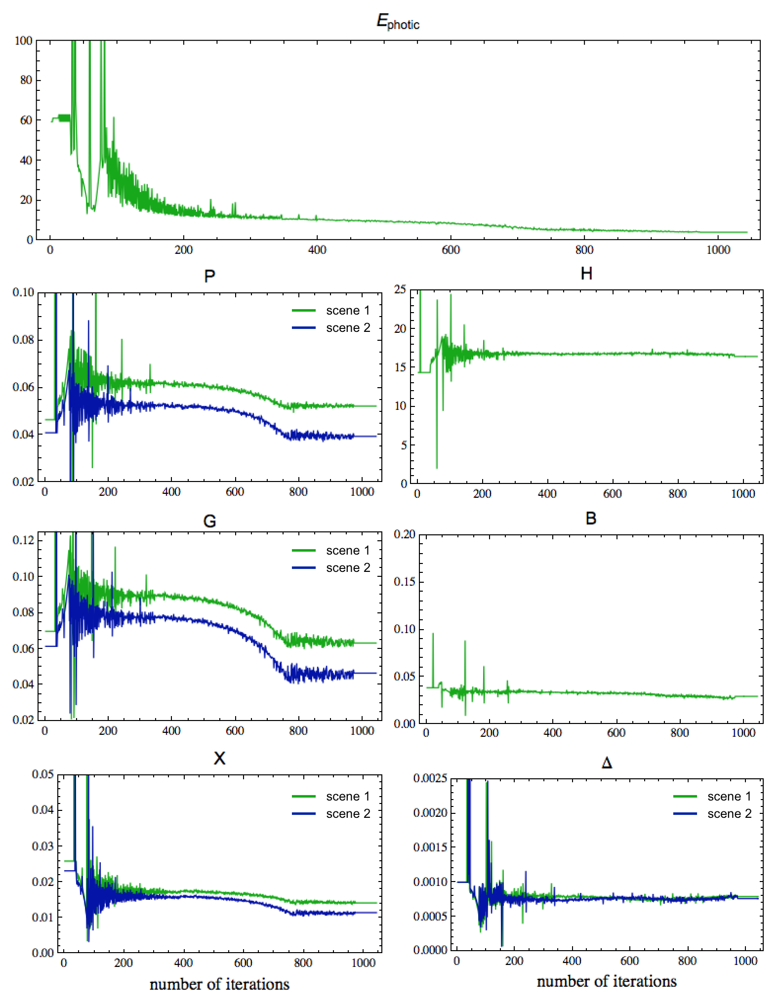
Figure 2: A plot of the path taken by each model variable during the minimisation process at the central modelled spectra.

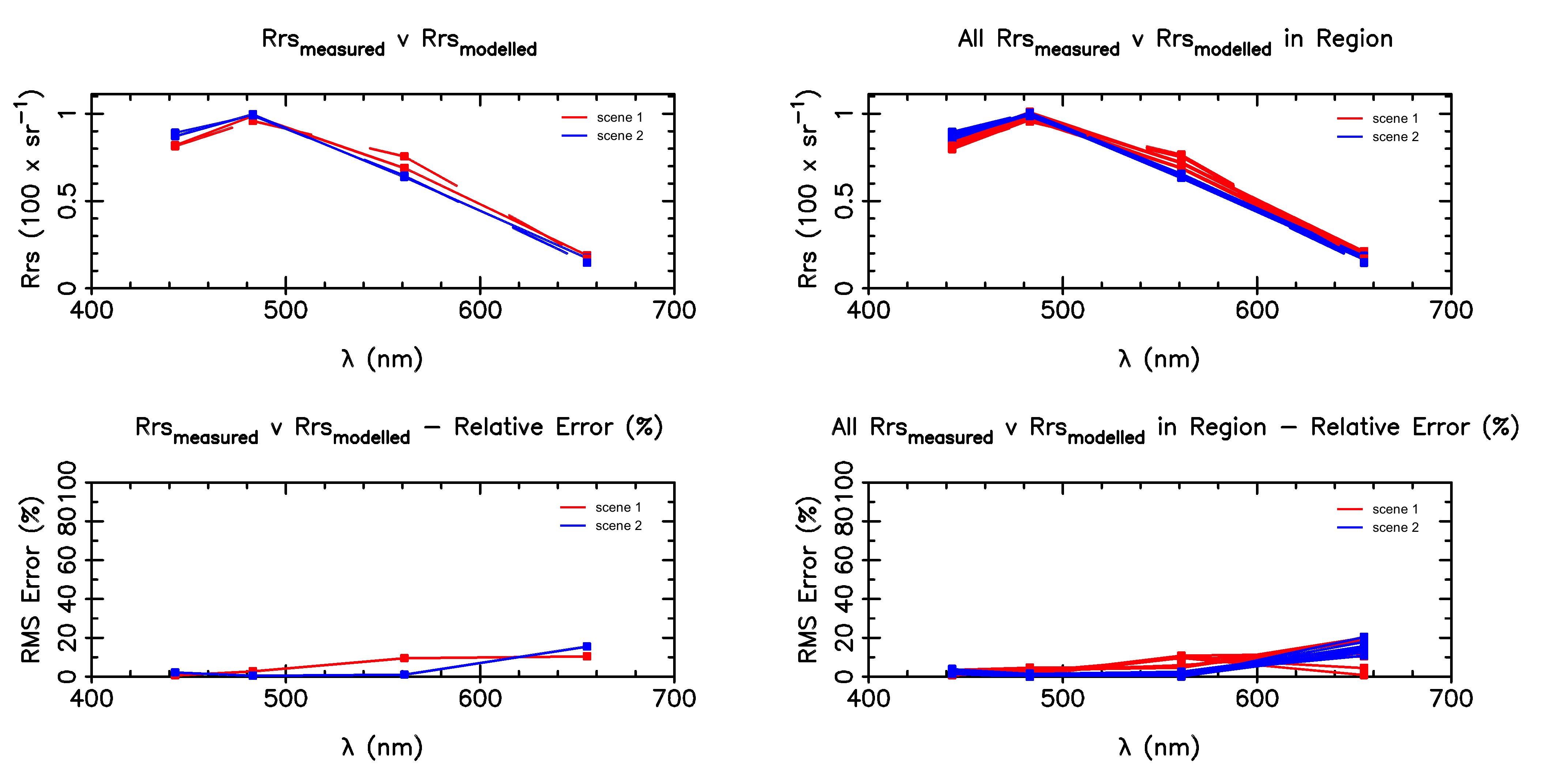
Figure 3: A plot comparing $R_{rs_{\text{measured}}}$ with $R_{rs_{\text{modelled}}}$ at the central modelled spectra and at all $N_{r}$ surrounding spectra in the region.

In summary, the model required 1043 iterations to converge to a model error of $E_{\text{photic}}=3.96\%$. The derived parameters were

P $$=\left[0.05226967,0.03944374\right]$$

G $$=\left[0.06326824,0.04656528\right]$$

X $$=\left[0.01420787,0.01148168\right]$$

$$\mathbf{\Delta} =\left[0.00079306,0.00076364\right]$$

B $$=\left[0.0248,0.0295,0.0287,0.0299,0.0296,0.0293,0.0264,0.0264,0.0290\right]$$

H $$=\left[16.12,18.52,17.37,15.20,16.47,18.37,18.49,17.74,18.32\right]$$

Thus, the model-derived depth is 16.47 m.

5 Iterative Estimation of Depth, Water Turbidity and Bottom Composition

5.1 The first approximation

In the first approximation to the inversion, we model all individual scenes, pairs of scenes, 3-tuples of scenes and 4-tuples of scenes. In each of these modelling iterations, all parameters P, G, X, $\textbf{B}_{0}$, $\textbf{B}_{1}$, $\cdots$, $\textbf{B}_{N_{b}-1}$, $\textbf{q}_{0}$, $\textbf{q}_{1}$, $\cdots$, $\textbf{q}_{N_{b}-1}$, H and $\mathbf{\Delta}$ are estimated by the model and stored for subsequent use.

5.2 Depth averaging

If reliable depth profiles are not known, then we take the median of all iterations of the singletons, pairs, 3- and 4-tuples from the first approximation above. We use a weighted median, where the weight is proportional to the number of scenes in the model. That is, proportional to $N_{s}$.

5.3 Aligning $H$, with known depth profiles

If reliable depth profiles are known, then the model-derived depths, $H$, can be aligned with these profiles. This technique, for a single scene, was used by Ohlendorf et al [32, Figure 9. Depth validation at Rottnest Island, 2005] as a post processing step to the model inversion.

From the $n$ model-derived depths, $H_{0},H_{1},\cdots,H_{n-1}$, we construct a single depth $H_{\text{aligned}}$, such that

$$H_{\text{aligned}}(c_{0},c_{1},\cdots,c_{n-1},a_{0},a_{1},\cdots a_{n-1},b_{0},b_{1},\cdots,b_{n-1})=\frac{\sum\limits_{i=0}^{n-1}c_{i}a_{i}H_{i}^{b_{i}}}{\sum\limits_{i=0}^{n-1}c_{i}},$$

where $c_{i},a_{i},b_{i}>0$. We construct the same weighting scheme as used in the empirical method - consider $N$ soundings $s_{0},s_{1},\cdots,s_{N-1}$, we begin by generating weights for each soundings $w_{0},w_{1},\cdots,w_{N-1}$ such that

$$w_{i}=1-W_{i}/M,\quad\text{where}\quad W_{i}=\sum\limits_{j=0}^{N-1}e^{\left(s_{i}-s_{j}\right)^{2}},$$

where $M=\max(W_{0},W_{1},\cdots,W_{N-1})$. We construct a weighted, root-mean-square, relative error metric, $E_{\text{aligned}}$, such that

$$E_{\text{aligned}}(c_{0},c_{1},\cdots,c_{n-1},a_{0},a_{1},\cdots a_{n-1},b_{0},b_{1},\cdots,b_{n-1})=\sqrt{\frac{\sum\limits_{i=0}^{N-1}w_{i}\left(\frac{H_{\text{aligned}_{i}}-s_{i}}{s_{i}}\right)^{2}}{\sum\limits_{i=0}^{N-1}w_{i}}}$$

where $H_{\text{aligned}_{i}}$ is shorthand for $H_{\text{aligned}}(c_{0},c_{1},\cdots,c_{n-1},a_{0},a_{1},\cdots a_{n-1},b_{0},b_{1},\cdots,b_{n-1})$ at the spatial location of the sounding, $s_{i}$.

To find the minima of $E_{\text{aligned}}$, we use the simplex algorithm [2] with an initial simplex of $c_{i},a_{i},b_{i}=1$ for all $i$. If the model is well calibrated, then we expect this starting point to be close to the minima.

5.4 Averaging $k$

If the modelled attenuation coefficients, $k(\lambda)$ (eqn. 2.2), is relatively constant over time, then we can average $k(\lambda)$ over all model iterations from 5.1. Otherwise all individual model-derived parameters can be averaged.

5.5 Deriving bottom types

We perform an additional optimisation iteration to improve the accuracy of the unmixing of multiple bottom types. In this modelling iteration we use the previously estimated P, G, X, $\textbf{B}_{0}$, $\textbf{B}_{1}$, $\cdots$, $\textbf{B}_{N_{b}-1}$, H and $\mathbf{\Delta}$. However, P, G, X and $\mathbf{\Delta}$ are constant. We use the values of $\textbf{B}_{0}$, $\textbf{B}_{1}$, $\cdots$, $\textbf{B}_{N_{b}-1}$ as an initialisation for subsequent modelling.

We begin by expressing 2.1 in terms of $\rho(\lambda)$, which we term $\rho_{\text{modelled}}(\lambda)$ with parameters $P$, $G$, $X$, $H$, $\Delta$

$$\rho_{\text{modelled}}(P,G,X,H,\Delta,\lambda)=\pi\exp\left(\left(\frac{1}{\cos(\theta_{\text{sun}})}+\frac{D_{B}(\lambda)}{\cos(\theta_{\text{view}})}\right)\,k(\lambda)\,H\right)\bigg{[}r_{rs}(\lambda)-\\ \left.r_{rs_{\infty}}(\lambda)\left(1-\exp\left(-\left(\frac{1}{\cos(\theta_{\text{sun}})}+\frac{D_{C}(\lambda)}{\cos(\theta_{\text{view}})}\right)\,k(\lambda)\,H\right)\right)\right].$$

where

$$r_{rs}(\lambda)=\frac{2(R_{rs}(\lambda)-\Delta)}{1+3(R_{rs}(\lambda)-\Delta)}$$

and the corresponding unmixed $\rho(\lambda)$, which we term $\rho_{\text{unmixed}}(B_{0},B_{1},\cdots,B_{N_{b}-1},q_{0},q_{1},\cdots,q_{N_{b}-1},\lambda)$ is given by

$$\rho_{\text{unmixed}}(B_{0},B_{1},\cdots,B_{N_{b}-1},q_{0},q_{1},\cdots,q_{N_{b}-1},\lambda)=\frac{\sum\limits_{i=0}^{N_{b}-1}B_{i}\,q_{i}\,\rho_{\text{bottom}_{i}}(\lambda)}{\sum\limits_{i=0}^{N_{b}-1}q_{i}}.$$

Then we use the averaged (or aligned) depths as H across all subsequent model iterations. The values of P, G, X, $\mathbf{\Delta}$ are averaged across all previous modelling iterations from 5.1 for each scene. If noise is present in these datasets then we apply a median filter, prior to computing $\rho_{\text{modelled}}$.

In this modelling iteration we keep P, G, X, H, $\mathbf{\Delta}$ static and optimise only for $\textbf{B}_{0}$, $\textbf{B}_{1}$, $\cdots$, $\textbf{B}_{N_{b}-1}$, $\textbf{q}_{0}$, $\textbf{q}_{1}$, $\cdots$, $\textbf{q}_{N_{b}-1}$. As previously, we assume the bottom spectra do not change over time, this allows us to simultaneously model multiple scenes. We index the $N_{s}$ scenes, with $j$.

The error metric for the unmixing is given by

$$E_{\text{unmixed}}\left(\textbf{B}_{0},\textbf{B}_{1},\cdots,\textbf{B}_{N_{b}-1},\textbf{q}_{0},\textbf{q}_{1},\cdots,\textbf{q}_{N_{b}-1}\right)=E^{\text{RMS}}_{\text{unmixed}}\,E^{\text{SAM}}_{\text{unmixed}},$$

where

$$E^{\text{RMS}}_{\text{unmixed}}\left(\textbf{B},\textbf{q}_{0},\textbf{q}_{1},\cdots,\textbf{q}_{N_{b}-1}\right)=\frac{\sqrt{\sum\limits_{j=0}^{N_{s}-1}\sum\limits_{\lambda}\left(\rho_{\text{unmixed}}^{j}-\rho_{\text{modelled}}^{j}\right)^{2}}}{\sum\limits_{j=0}^{N_{s}-1}\sum\limits_{\lambda}\rho_{\text{modelled}}^{j}}$$

and

$$E^{\text{SAM}}_{\text{unmixed}}\left(\textbf{B}_{0},\textbf{B}_{1},\cdots,\textbf{B}_{N_{b}-1},\textbf{q}_{0},\textbf{q}_{1},\cdots,\textbf{q}_{N_{b}-1}\right)=\\ \frac{1}{N_{s}}\sum\limits_{j=0}^{N_{s}-1}\cos^{-1}\left(\frac{\rho_{\text{unmixed}}^{j}\cdot\rho_{\text{modelled}}^{j}}{\left(\rho_{\text{unmixed}}^{j}\cdot\rho_{\text{unmixed}}^{j}\right)\left(\rho_{\text{modelled}}^{j}\cdot\rho_{\text{modelled}}^{j}\right)}\right),$$

where $\rho_{\text{unmixed}}^{j}$ is shorthand for $\rho_{\text{unmixed}}^{j}(B_{0},B_{1},\cdots,B_{N_{b}-1},,q_{0},q_{1},\cdots,q_{N_{b}-1},\lambda)$ and $\rho_{\text{modelled}}^{j}$ is shorthand for $\rho_{\text{modelled}}^{j}(P,G,X,H,\Delta,\lambda)$.

5.6 Depth error estimate

Obtaining a realistic depth error estimate requires accounting for uncertainties in both the model inputs and the model itself.

We estimate the sensor noise by computing the RRS standard deviation in optically deep water. The model then adds (or subtracts) random noise within the threshold of the estimated sensor noise. The corresponding standard deviation of the resulting depths over many trials is the depth error estimate.

We can further account for errors in the model, bottom reflectance, absorption and backscattering spectra by scaling the depth error estimate, if reasonable upper bounds on the error estimates of these quantities are known.

6 Case Study – Murion Island Marine Management Area

As a small exemplar case study we modelled a 260 $\text{km}^{2}$ region to the south of North Murion Island, including Sunday Island, Combe Reef and Exmouth Reef; which are off the Pilbara Coast in Western Australia. This area is part of the Murion Island Marine Management Area. It is also an important area for commercial marine traffic.

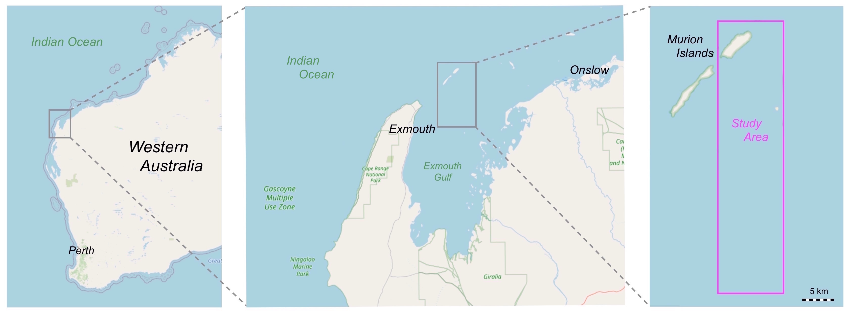
Figure 4: A map showing the location of the study area in northern Western Australia [37].

A single-beam sonar survey was conducted in 2011 by Transport WA. Within the spatial domain of this case study there are 53 194 sonar measurements, the majority of which are between depths of 12 and 22 m. This survey is approximately 32 km by 9.5 km.

The satellite imagery used for this study was from the LANDSAT 8 satellite. The scenes from this satellite are $170\,\text{km}\times 185\,\text{km}$ in size at a horizontal resolution of approximately 30 m. The USGS provides open access to the entire archive of LANDSAT imagery dating back to 1972. In total, 4 scenes were selected for modelling

Table 4: LANDSAT-8 scenes used in the case study.

study ID	scene ID	WRS-2 path	WRS-2 row	date	sun elevation
1	LC81150752015210LGN02	115	75	2015-07-29	38.86∘
2	LC81150752018058LGN00	115	75	2018-02-27	55.22∘
3	LC81150752018266LGN00	115	75	2018-09-23	54.85∘
4	LC81150752019253LGN00	115	75	2019-09-10	50.68∘

Atmospheric correction and sun glint correction was performed with ACOLITE [36].

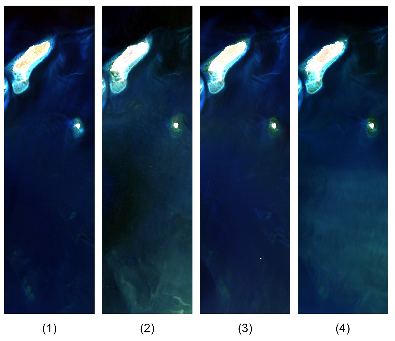
Figure 5: Natural colour images of the 4 atmospherically-corrected LANDSAT-8 scenes used in this case study; labelled by scene ID. It is visually evident that scenes 2 and 4 exhibit higher turbidity in the southern area of the case study. In scene 3 a large vessel is present within the AOI.

The bottom types used in this study were sand, seagrass and coral. Unfortunately, these spectra were not collected from the study site and at best can only be used as approximate representative samples.

Depth soundings used for the initial depth estimation were digitised from chart WA 900 - Point Murat to North Murion Island. The empirical model (see section 4.1) performed well, with a mean relative error of 15% and a mean absolute error of 1.74 m.

photic was parameterised with $N_{r}=9$, $N_{s}=1,2,3,4$, $N_{b}=3$. In total, we modelled 15 combinations of these 4 scenes. Where the combinations of modelled scenes, by study ID, were [1], [2], [3], [4], [1,2], [1,3], [1,4], [2,3], [2,4], [3,4], [1,2,3], [1,2,4], [1,3,4], [2,3,4], [1,2,3,4]. The final depth was taken as the spatial median of the 15 modelling iterations.

All 15 model iterations of photic ran sequentially in 5 hours. The lookup table accounted for modelling the majority of the points. Without the lookup table the modelling would have taken around two weeks (running sequentially on a single core).

In the scatter plot below a vertical correction of -0.75 m was applied to the model-derived bathymetry. This accounts for tidal variations and a correction to the vertical datum of the sonar data.

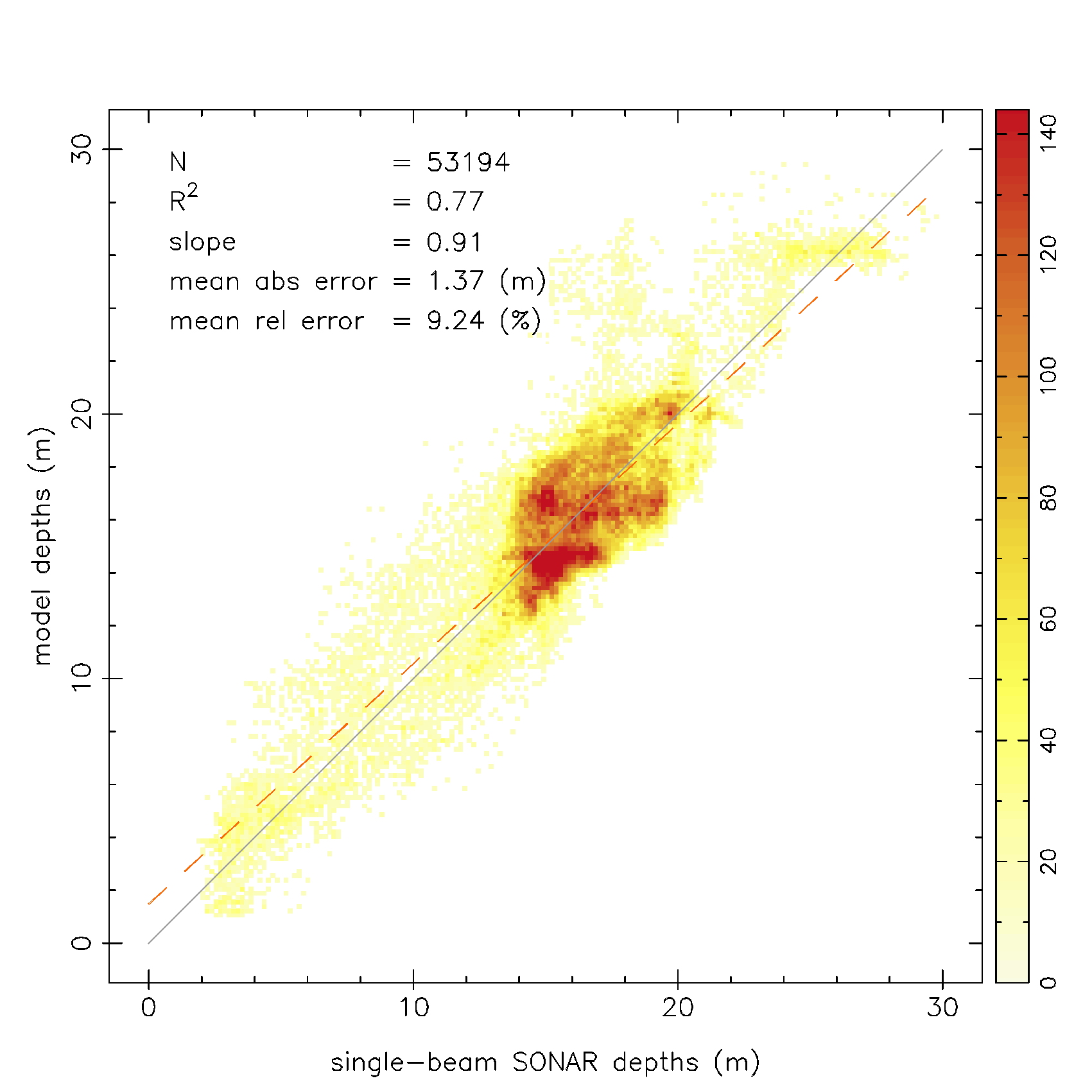
Figure 6: A scatter (density) plot of the 2011 single-beam sonar bathymetry survey with the LANDSAT-derived bathymetry.

The regression analysis between the sonar survey and the LANDSAT-derived bathymetry shows good agreement, with $N=53\,194$, $R^{2}=0.77$, the least squares line of best fit was $y=0.91x+1.61$, the mean absolute error was 1.17 m, and the mean relative error was 7.52%. Furthermore, below we give a summary of the absolute and relative errors.

Table 5: Summary of absolute and relative percentage errors.

9.94% within 0.25 m 20.20% within 0.50 m 31.59% within 0.75 m 42.86% within 1.00 m 62.58% within 1.50 m 76.79% within 2.00 m			12.51% within 2.00 (rel % error) 33.10% within 5.00 (rel % error) 64.89% within 10.00 (rel % error) 85.21% within 15.00 (rel % error) 94.62% within 20.00 (rel % error) 96.42% within 25.00 (rel % error)

The LANDSAT-derived bathymetry correlates well with the single-beam sonar data. While it is difficult to compare studies in different regions, the regression analysis suggests our model-derived bathymetry has similar performance to other physics-based, model-derived bathymetry [32][30]. We do not, however see LANDSAT 8 or Sentinel-2 data competing with hyperspectral data in terms of accuracy of bathymetric retrieval.

In the following graphic we display the key model-derived datasets and the model derived parameterisation of P, G and X.

Figure 7: A plot of (a) the sonar depths; (b) the model-derived depths, comprising the median of all 15 model iterations; (c) the one sigma depth error estimate; (d) the minimum attenuation coefficient, averaged over all 15 model iterations; (e) the model-derived bottom albedo (the parameter $B$ from (2.4)); (f) the model error, $E_{\text{photic}}$, averaged over all 15 model iterations.

Figure 8: A plot of P, G and X for scenes LC81150752015210LGN02 and LC81150752018058LGN00. In each of these plots we have taken the median of the 15 model iterations.

Figure 9: A plot of P, G and X for scenes LC81150752018266LGN00 and LC81150752019253LGN00. In each of these plots we have taken the median of the 15 model iterations.

It is of interest to see the increase in $E_{\text{photic}}$ in a band to the south of North Murion Island (plot (f) above). This coincides with a sharp drop-off in depth and consequently is can be explained by the model trying to minimise both the RRS error and the depth continuity error (3.2). As the RRS error is significantly higher weighted than the depth continuity error, the model will favour the minimisation of the RRS error in such cases. Otherwise, the average error is well below 5%, which is expected.

The range of H-sigma is reasonable, as this estimate does not include uncertainties introduced in the estimation of the bottom spectra, atmospheric correction, and core assumptions within the original model of Lee et al.

When interpreting the range of the mean, minimum attenuation coefficient it must be considered that the 4 scenes were selected amongst over 100 scenes for their minimal water turbidity.

One region where upon visual inspection the model-derived bathymetry performs poorly is directly east of North Murion Island. Below we have plotted the sonar data over the model-derived bathymetry. This may be due to a shift in the seabed in the 9 years since the sonar survey was conducted (unlikely) or due to poorly estimating the bottom reflectance in this area (likely).

Figure 10: A region east of North Murion Island (highlighted with a pink rectangle) where the model-derived bathymetry performs poorly. The single-bean sonar data is displayed over the model-derived bathymetry.

By way of comparison, we modelled each scene individually with the spatial and temporal extensions removed ($N_{r}=1$, $N_{s}=1$). We also removed the initial depth estimates and the lookup table. The resulting model-derived bathymetry clearly shows instabilities in the optimisation scheme with so few data points to perform the fit.

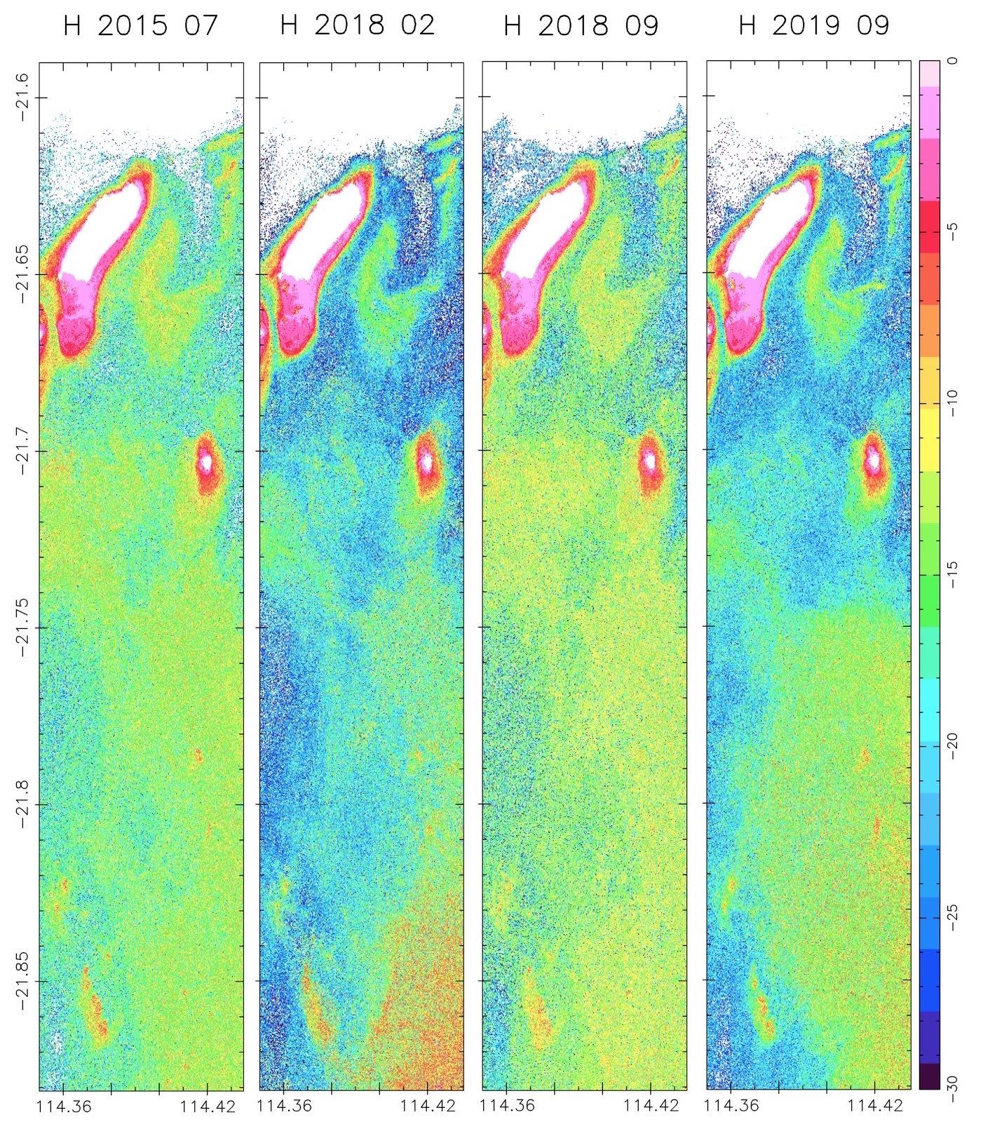
Figure 11: Plot of the model-derived bathymetry with the parameterisation $N_{r}=1$, $N_{s}=1$, $N_{b}=3$, and the initial depth estimates and lookup table removed from the model.

7 Conclusions & Future Work

In this paper we have shown that multispectral imagery can be used successfully within a physics-based. We have made temporal and spatial extensions to the model of Lee et al [14][15][16], which increase the stability and accuracy of depth retrievals when using low spectral resolution satellites like LANDSAT 8 or Sentinel-2.

Further work is underway to sort the spectra into clusters, where in each cluster only a small fraction of the spectra require modelling due to their spectral similarity.

Appendix A Appendix

From the model of Lee for $a_{\phi}(\lambda)=\left(a_{0}(\lambda)+a_{1}(\lambda)\log(P)\right)P$, we derived (using least-squares, non-linear optimisation) $a_{0}$ and $a_{1}$ using a dataset collected by the CSIRO in 2003–2005 near Bunbury, Western Australia [21]. This dataset comprised 71 measurements and collected in depths ranging from 1.5 to 20 m.

Table 6: 440nm-normalised $a_{0}$, $a_{1}$ derived from the Bunbury, Western Australia field measurements.

$\lambda$	$a_{0}$	$a_{1}$	$\lambda$	$a_{0}$	$a_{1}$	$\lambda$	$a_{0}$	$a_{1}$
400	0.69322	0.01035	520	0.32875	0.00617	640	0.24139	0.02122
405	0.80506	0.01868	525	0.30033	0.00753	645	0.25922	0.02508
410	0.89891	0.02278	530	0.27633	0.00874	650	0.26483	0.02589
415	0.96392	0.02497	535	0.25874	0.01065	655	0.27135	0.02374
420	0.99268	0.02371	540	0.23621	0.01005	660	0.31442	0.02326
425	1.00392	0.01841	545	0.21342	0.00897	665	0.40322	0.02714
430	1.02963	0.01381	550	0.19724	0.00975	670	0.49153	0.03177
435	1.03967	0.00750	555	0.18247	0.01048	675	0.52301	0.03344
440	1.0	0.0	560	0.16819	0.01044	680	0.46490	0.02943
445	0.90067	-0.01143	565	0.15781	0.01023	685	0.33078	0.01968
450	0.79228	-0.02292	570	0.15495	0.01076	690	0.19484	0.01007
455	0.74203	-0.02655	575	0.15478	0.01080	695	0.11332	0.00577
460	0.74870	-0.02273	580	0.15795	0.01102	700	0.07804	0.00588
465	0.76773	-0.01590	585	0.16251	0.01104	705	0.05617	0.00477
470	0.77611	-0.00746	590	0.16427	0.01054	710	0.04426	0.00401
475	0.76177	-0.00132	595	0.16247	0.01027	715	0.03844	0.00414
480	0.72663	-0.00007	600	0.16094	0.01062	720	0.03209	0.00361
485	0.68161	-0.00094	605	0.16188	0.01104	725	0.02705	0.00333
490	0.63211	-0.00109	610	0.16489	0.01075	730	0.02090	0.00253
495	0.57497	-0.00056	615	0.17238	0.01088	735	0.02198	0.00528
500	0.51537	0.00073	620	0.17878	0.01073	740	0.01671	0.00383
505	0.45850	0.00244	625	0.18479	0.01090	745	0.00866	0.00191
510	0.40764	0.00391	630	0.19970	0.01329	750	0.01262	0.00288
515	0.36526	0.00529	635	0.21805	0.01636

Below we compare our derived $a_{0}$, $a_{1}$ with the original parameterisation of Lee [10] and Lee et al [14] against 12 of the collected samples.

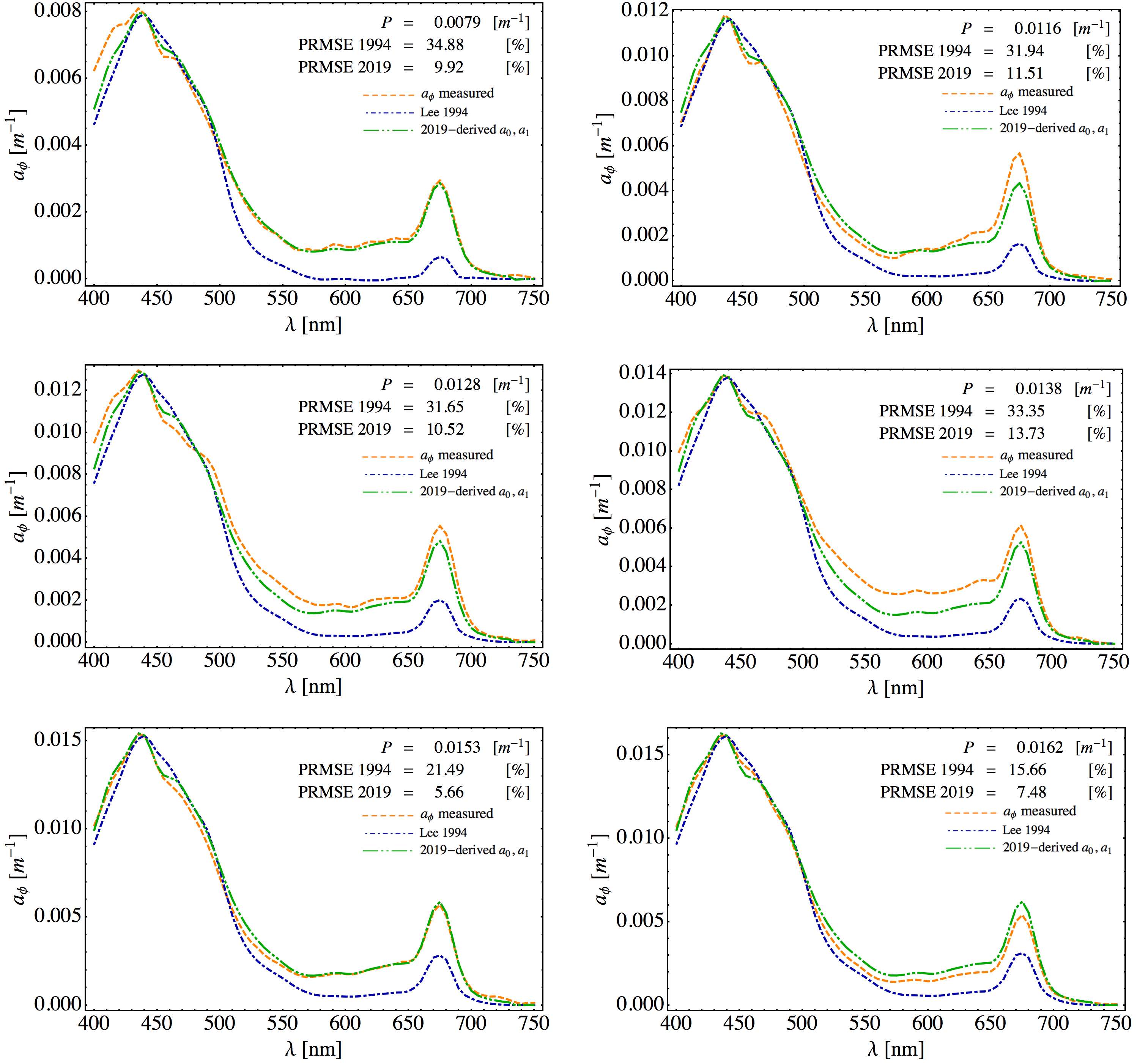
Figure 12: A plot comparing the measured and modelled $a_{\phi}$ for the original parameterisation of Lee and the Bunbury-derived $a_{0}$, $a_{1}$.

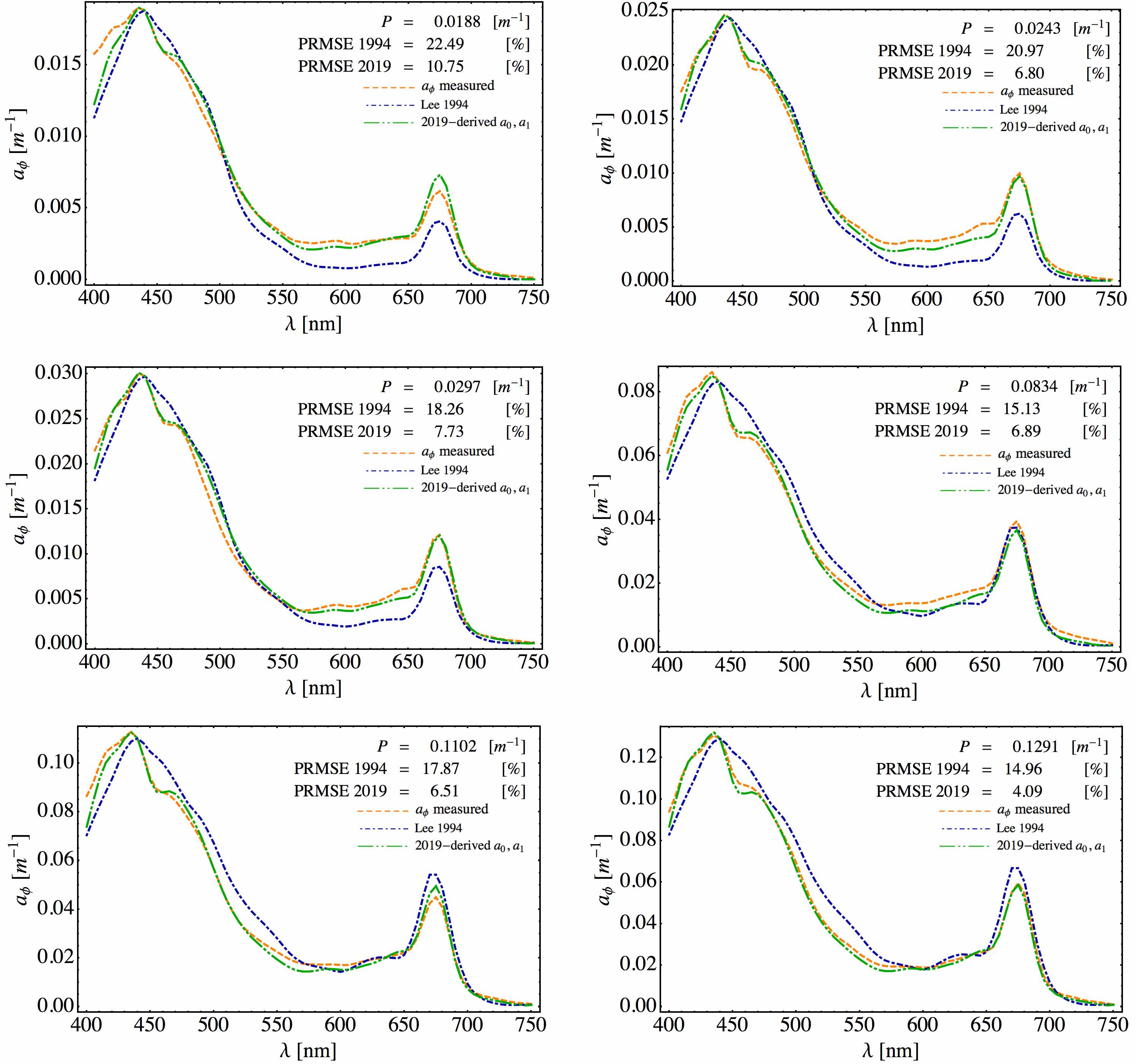
Figure 13: A plot comparing the measured and modelled $a_{\phi}$ for the original parameterisation of Lee and the Bunbury-derived $a_{0}$, $a_{1}$.

References

- [1] F.C. Polcyn, W.L. Brown, I.J. Sattinger, “The Measurement of Water Depth by Remote Sensing Techniques”, Spacecraft Oceanography Project, US Naval Oceanographic Office, Washington DC, 1970
- [2] R. O’Neil, “Algorithm AS 47: Function Minimization Using a Simplex Procedure”, Journal of the Royal Statistical Society. Series C (Applied Statistics), vol. 20, no. 3, pp. 338–345, 1971
- [3] A. Morel, “Optical properties of pure water and pure sea waters”, Optical Aspects of Oceanography, N. G. Jerlov and E. S.Nielsen, eds. Academic, pp. 1–24, 1974
- [4] F.C. Polcyn, “NASA/COUSTEAU OCEAN BATHYMETRY EXPERIMENT - Remote Bathymetry Using High Gain LANDSAT data”, NASA, Goddard Space Fligh Center, 1976
- [5] N. Jerlov, “Optical Oceanography”, 1968
- [6] D.R. Lyzenga, “Passive remote sensing techniques for mapping water depth and bottom features”, Applied Optics, vol. 17, no. 3, pp. 379–383, 1978
- [7] https://science.nasa.gov/missions/geosat
- [8] H.R. Gordon et al, “A semianalytical radiance model of ocean color”, Journal of Geophysical Research, vol. 93, pp. 10909–10942, 1988
- [9] S. Maritorena, A. Morel, B. Gentili, “Diffuse reflectance of oceanic shallow waters: Influence of water depth and bottom albedo”, American Society of Limnology and Oceanography, vol. 39, no. 7, pp. 1689–1703, 1994
- [10] Z. P. Lee, “Visible-infrared remote-sensing model and applications for ocean waters”, Ph.D. dissertation, Department of Marine Science, University of South Florida, 1994
- [11] A. Lawler, “Sea-Floor Data Flow From Postwar Era”, Science, vol. 270, issue 5237, pp. 727, November 1995
- [12] R. Pope, E. Fry, “Absorption spectrum 380–700 nm of pure waters: II. Integrating cavity measurements”, Applied Optics, vol. 36, pp. 8710–8723, 1997
- [13] Y. Morel, L.T. Lindell, “PASSIVE MULTISPECTRAL BATHYMETRY MAPPING OF NEGRIL SHORES, JAMAICA”, Fifth International Conference on Remote Sensing for Marine and Coastal Environments, San Diego, California, October 1998
- [14] Z. Lee et al, “Hyperspectral remote sensing for shallow waters. I. A semianalytical model”, Applied Optics, vol. 37, no. 27, pp. 6329–6338, 1998
- [15] Z. Lee et al, “Hyperspectral remote sensing for shallow waters: 2. Deriving bottom depths and water properties by optimization”, Applied Optics, vol. 38, no. 18, pp. 3831–3843, 1999
- [16] Z. Lee et al, “Properties of the water column and bottom derived from Airborne Visible Infrared Imaging Spectrometer (AVIRIS) data”, Journal of Geophysical Research, vol. 106, no. C6, pp. 11639–11651, June 2001
- [17] Z. Lee, K.L. Carder, “Effect of spectral band numbers on the retrieval of water column and bottom properties from ocean color data”, Applied Optics, vol. 41, no. 12, pp. 2191–2201, April 2002
- [18] A. Albert, C.D. Mobley, “An analytical model for subsurface irradiance and remote sensing reflectance in deep and shallow case-2 waters”, Optics Express, vol. 11, no. 22, pp. 2873–2890, 2003
- [19] P. Gege, “The water color simulator WASI: an integrating software tool for analysis and simulation of optical in situ spectra”, Computers & Geosciences, vol. 30, pp. 523–532, 2004
- [20] W.M. Klonowski, L.J. Majewski, P.R.C.S. Fearns, L.A. Clementson, M.J. Lynch, 2004. “Bottom type classification using hyperspectral imagery”, Proceedings Ocean Optics XVII (CDROM), 2004
- [21] R. Babcock, L. Clementson, Bunbury Deployment 2003–2005: absorption-phytoplankton data, Integrated Marine Observing System (IMOS), https://portal.aodn.org.au/, CSIRO, 2003–2005
- [22] A. Albert, P. Gege, “Inversion of irradiance and remote sensing reflectance in shallow water between 400 and 800 nm for calculations of water and bottom properties”, APPLIED OPTICS, vol. 45, no. 10, pp. 2331–2343, April 2006
- [23] C.D. Mobley et al, “Interpretation of hyperspectral remote-sensing imagery by spectrum matching and look-up tables”, Applied Optics, vol. 44, no. 17, pp. 3576–3592, 2005
- [24] D.R. Lyzenga, N.P. Malinas, F.J. Tanis, “Multispectral Bathymetry Using a Simple Physically Based Algorithm”, IEEE Transactions on Geoscience and Remote Sensing, vol. 44, no. 8, 2006
- [25] M. Wettle, V.E. Brando, “SAMBUCA Semi-Analytical Model for Bathymetry, Un-mixing, and Concentration Assessment”, CSIRO Land and Water Science Report 22/06, July 2006
- [26] W.M. Klonowski, P.R.C.S. Fearns, M.J. Lynch, “Retrieving key benthic cover types and bathymetry from hyperspectral imagery”, Journal of Applied Remote Sensing, vol. 1, 011505, 2007
- [27] Z. Lee, “Test, Evaluate, and Characterize a Remote-Sensing Algorithm for Optically-Shallow Waters”, Geosystems Research Institute, Northern Gulf Institute, Mississippi State University, Stennis Space Center, 2009
- [28] J. Hedley, C. Roelfsema, S. Phinn, “Efficient radiative transfer model inversion for remote sensing applications”, Remote Sensing of the Environment, vol. 133, issue 11, pp. 2527–2532, November 2009
- [29] V.E. Brando, J.M. Anstee, M. Wettle, A.G. Dekker, S.R. Phinn, C. Roelfsema, “A physics based retrieval and quality assessment of bathymetry from suboptimal hyperspectral data”, Remote Sensing of the Environment, vol. 113, issue 4, pp. 755–770, 2009
- [30] S. Sagar, M. Wettle, “Mapping the fine-scale shallow water bathymetry of the Great Barrier Reef using ALOS AVNIR-2 data”, OCEANS 2010 IEEE - Sydney
- [31] Z. Lee, “Global Shallow-Water Bathymetry From Satellite Ocean Color Data”, EOS, vol. 91, no. 46, 16 November 2010
- [32] S. Ohlendorf, A. Muller, T. Heege, S. Cerdeira-Estrada, H.T. Kobryn, “Bathymetry mapping and sea floor classification using multispectral satellite data and standardized physics-based data processing”, Remote Sensing of the Ocean, Sea Ice, Coastal Waters, and Large Water Regions, Prague, September 2011
- [33] A. Dekker et al, “Intercomparison of shallow water bathymetry, hydro-optics, and benthos mapping techniques in Australian and Caribbean coastal environments”, Limnology and Oceanography: Methods, vol. 9, pp. 396–425, 2011
- [34] A.G. Dekker, S. Sagar, V.E. Brando, D. Hudson, “Bathymetry from satellites for hydrographic purposes”, Shallow Survey 2012, Wellington, New Zealand, February 2012
- [35] J.D. Hedley, et al, “Coral reef applications of Sentinel-2: Coverage, characteristics, bathymetry and benthic mapping with comparison to Landsat 8”, Remote Sensing of Environment, vol. 216, pp. 598–614.
- [36] Q. Vanhellemont, “Adaptation of the dark spectrum fitting atmospheric correction for aquatic applications of the Landsat and Sentinel-2 archives”, Remote Sensing of Environment, vol. 225, pp. 175–192, 2019. (https://doi.org/10.1016/j.rse.2019.03.010)
- [37] OpenStreetMap contributors, https://www.openstreetmap.org/