Analytical solution for the spectrum of two ultracold atoms in a completely anisotropic confinement

Abstract

We study the system of two ultracold atoms in a three-dimensional (3D) or two-dimensional (2D) completely anisotropic harmonic trap. We derive the algebraic equation $J_{\rm 3D}(E)=1/a_{\rm 3D}$ ($J_{\rm 2D}(E)=\ln a_{\rm 2D}$) for the eigen-energy $E$ of this system in the 3D (2D) case, with $a_{\rm 3D}$ and $a_{\rm 2D}$ being the corresponding $s$-wave scattering lengths, and provide the analytical expressions of the functions $J_{\rm 3D}(E)$ and $J_{\rm 2D}(E)$. In previous researches this type of equation was obtained for spherically or axially symmetric harmonic traps (T. Busch, et. al., Found. Phys. 28, 549 (1998); Z. Idziaszek and T. Calarco, Phys. Rev. A 74, 022712 (2006)). However, for our cases with a completely anisotropic trap, only the equation for the ground-state energy of some cases has been derived (J. Liang and C. Zhang, Phys. Scr. 77, 025302 (2008)). Our results in this work are applicable for arbitrary eigen-energy of this system, and can be used for the studies of dynamics and thermal-dynamics of interacting ultracold atoms in this trap, e.g., the calculation of the 2nd virial coefficient or the evolution of two-body wave functions. In addition, our approach for the derivation of the above equations can also be used for other two-body problems of ultracold atoms.

I Introduction

The two-body problems of trapped interacting ultracold atoms are basic problems in cold atom physics Busch et al. (1998); Idziaszek and Calarco (2005, 2006); Liang and Zhang (2008); Blume (2012); Grishkevich and Saenz (2009); Grishkevich et al. (2011); Sala et al. (2013); Sala and Saenz (2016); Sun et al. (2006); Kehrberger et al. (2018); Bougas et al. (2019); Budewig et al. (2019). They are of broad interest because of the following reasons. First, the two-body systems are “minimum” interacting systems of trapped ultracold atoms, and one can obtain a primary understanding for the interaction physics of an ultracold gas from the analysis of such systems Wenz et al. (2013). Second, the solutions to these problems can be directly used to calculate some important few- or many-body quantities Blume and Greene (2002); Liu et al. (2009); von Stecher et al. (2008); Daily and Blume (2010); Gharashi et al. (2012); Liu (2013); Yin et al. (2014a, b); Peng et al. (2014); Yin and Blume (2015); Blume et al. (2018); Yin et al. (2020), e.g., the 2nd virial coefficient which determines the high-temperature properties of the ultracold gases. Third, these systems have been already realized in many experimentsWenz et al. (2013); Scazza et al. (2014); Cappellini et al. (2014); Norcia et al. (2018); Cooper et al. (2018); Cappellini et al. (2019); Guan et al. (2019); Liu et al. (2018); Anderegg et al. (2019); Hood et al. (2019); Wang et al. (2019); Chang et al. (2018); Meng et al. (2018); Dareau et al. (2018) where the trap of the two atoms can be created via an optical lattice site Scazza et al. (2014); Cappellini et al. (2014, 2019), an optical tweezer Guan et al. (2019); Liu et al. (2018); Anderegg et al. (2019); Hood et al. (2019); Wang et al. (2019), or nano-structure Chang et al. (2018); Meng et al. (2018); Dareau et al. (2018). In these experiments, by measuring or controlling the energy spectrum or dynamics of these two atoms, one can, e.g., create a cold molecule in an optical tweezer Liu et al. (2018); Anderegg et al. (2019), derive the parameters of inter-atomic interaction potential Scazza et al. (2014); Cappellini et al. (2014, 2019); Hood et al. (2019) or study various dynamical effects such as the interaction-induced density oscillation Guan et al. (2019). Theoretical results for the corresponding two-body problems are very important for these experimental studies.

The most fundamental systems of two trapped ultra-cold atoms are the ones with a harmonic trap which has the same frequencies for each atom, and a $s$-wave short-range inter-atomic interaction. For these systems, the center-of-mass (CoM) and relative motion of the two atoms can be decoupled with each other, and the CoM motion is just the same as a harmonic oscillator. Nevertheless, the dynamics of the relative motion of these two atoms is nontrivial. For the three-dimensional (3D) systems, T. Busch, et. al. Busch et al. (1998) and Z. Idziaszek and T. Calarco Idziaszek and Calarco (2006, 2005) studied the cases with a spherically and axially symmetric harmonic trap, respectively. They show that the eigen-energy $E$ of the relative motion satisfies an algebraic equation with the form

$$J_{{\rm 3D}}(E)=\frac{1}{a_{{\rm 3D}}},$$ (1)

with $a_{{\rm 3D}}$ being the 3D $s$-wave scattering length, and provided the analytical expressions of the function $J_{{\rm 3D}}(E)$ for these two cases Busch et al. (1998); Idziaszek and Calarco (2006, 2005), as shown in Table I, respectively. Moreover, for the two-dimensional (2D) systems with an isotropic harmonic trap, T. Busch, et. al. obtained the equation

type	$E$	$J_{{\rm 3D}}(E)$	Ref.
$\omega_{x}=\omega_{y}=\omega_{z}$	arbitrary $E$	$\sqrt{2}\frac{\Gamma\left(-\frac{E}{2}+\frac{3}{4}\right)}{\Gamma\left(-\frac{E}{2}+\frac{1}{4}\right)}$	Ref. Busch et al. (1998)
$\omega_{x}=\omega_{y}\neq\omega_{z}$	arbitrary $E$	$-\frac{\eta_{x}}{\sqrt{2}}\sum\limits_{n={0}}^{\infty}\left[\frac{\Gamma\left(-\frac{E-E_{0}}{2}+n\eta_{x}\right)}{\Gamma\left(\frac{1}{2}-\frac{E-E_{0}}{2}+n\eta_{x}\right)}-\frac{1}{\sqrt{\eta_{x}}\sqrt{n+1}}\right]-\sqrt{\frac{\eta_{x}}{2}}\zeta\left(\frac{1}{2}\right)$	Ref. Idziaszek and Calarco (2006) $(\ast)$
$\omega_{x}\neq\omega_{y}\neq\omega_{z}$	$E<E_{0}$	$-\frac{1}{2\sqrt{\pi}}\int_{0}^{\infty}dt\left\{\frac{\sqrt{\eta_{x}\eta_{y}}\exp[{(E-E_{0})t}/{2}]}{\sqrt{1-e^{-\eta_{x}t}}\sqrt{1-e^{-\eta_{y}t}}\sqrt{1-e^{-t}}}-\frac{1}{t^{3/2}}\right\}$	Ref. Liang and Zhang (2008)
$\omega_{x}\neq\omega_{y}\neq\omega_{z}$	arbitrary $E$	Eq. (39) or Eq. (40)	this work

Table 1: Expressions of the function $J_{{\rm 3D}}(E)$ of Eq. (1) for various 3D traps. Here $\omega_{\alpha}$ ($\alpha=x,y,z$) is the trapping frequency in the $\alpha$-direction, and we use the natural unit $\hbar=2\mu=\omega_{z}=1$ with $\mu$ being the reduced mass of the two atoms. The parameters $\eta_{x}$ and $\eta_{y}$ are defined as $\eta_{x}=\omega_{x}/\omega_{z}$ and $\eta_{y}=\omega_{y}/\omega_{z}$, respectively, $E_{0}=(\eta_{x}+\eta_{y}+1)/2$ is the ground-state energy of the relative motion in the non-interacting case, and $\Gamma(z)$ and $\zeta(z)$ are the Gamma and Riemann zeta function, respectively. The two expressions (39) and (40) of $J_{\rm 3D}(E)$ given by this work are mathematically equivalent with each other. ($\ast$): Notice that there are typos in Eqs. (21, 23) of Ref. Idziaszek and Calarco (2006).

$$J_{{\rm 2D}}(E)=\ln a_{{\rm 2D}},$$ (2)

for the relative-motion eigen-energy $E$, where $a_{{\rm 2D}}$ is the 2D $s$-wave scattering length, and derive expression of the function $J_{{\rm 2D}}(E)$ Busch et al. (1998). With these results one can easily obtain the complete energy spectrum of these two-atom systems, as well as the corresponding eigen-states. Thus, these results have been widely used in the researches of cold atom physics Blume (2012); Wenz et al. (2013); Scazza et al. (2014); Cappellini et al. (2014, 2019); Hood et al. (2019); Ospelkaus et al. (2006); Stöferle et al. (2006); Mark et al. (2011); Riegger et al. (2018); Chapurin et al. (2019).

However, for two atoms trapped in a 3D completely anisotropic harmonic confinement, the algebraic equation for arbitrary eigen-energy of relative-motion has not been obtained so far. Only the equation of the ground-state energy of a system with positive scattering length has been obtained (i.e., the eigen-energy $E$ which satisfies $E<E_{0}$, with $E_{0}$ being the relative ground-state energy for the non-interacting case) in Ref. Liang and Zhang (2008), by J. Liang and C. Zhang in 2008. This equation has the form of Eq. (1), and the corresponding function $J_{\rm 3D}(E)$ is also shown in Table I. On the other hand, since this kind of confinements are easy to be experimentally prepared, and are thus used in many experiments of ultracold gases Scazza et al. (2014); Cappellini et al. (2014); Norcia et al. (2018); Cooper et al. (2018); Cappellini et al. (2019); Hood et al. (2019); Chapurin et al. (2019), it would be helpful if we can derive a general equation satisfied by all the eigen-energies.

In this work we derive the equation for arbitrary eigen-energy of two atoms in a completely anisotropic harmonic trap. We show that this equation also has the form of Eq. (1) and Eq. (2) for the 3D and 2D cases, respectively, and provide the corresponding analytical expressions of the functions $J_{{\rm 3D}}(E)$ (Table I) and $J_{{\rm 2D}}(E)$ (Eq. (61) or Eq. (63)). As the aforementioned results Busch et al. (1998); Idziaszek and Calarco (2006, 2005) for the spherically and axially symmetric traps, our equations are useful for the studies of various thermal-dynamcial or dynamical properties of ultracold gases in the completely anisotropic harmonic confinements. Furthermore, our calculation approach used in this work can also be generalized to other two-body problems of ultracold atoms in complicated confinements.

The remainder of this paper is organized as follows. In Sec. II and Sec. III, we derive the equations for eigen-energies of atoms in 3D and 2D completely anisotropic harmonic traps, respectively. In Sec. IV we discuss how to generalize our approach to other problems. A brief summary and some discussions are given in Sec. V. Some details of our calculations are shown in the appendix.

II 3D systems

We consider two ultracold atoms $1$ and $2$ in a 3D completely anisotropic harmonic trap which has the same frequencies for each atom. Here we denote $\omega_{\alpha}$ ($\alpha=x,y,z$) as the trapping frequency in the $\alpha$-direction, which satisfy

$$\omega_{x}\neq\omega_{y}\neq\omega_{z}.$$ (3)

For convenience, in this work we use the natural unit

$$\hbar=2\mu=\omega_{z}=1,$$ (4)

with $\mu$ being the reduced mass of the two atoms. We further introduce the aspect ratios

$$\eta_{x}=\frac{\omega_{x}}{\omega_{z}};\ \eta_{y}=\frac{\omega_{y}}{\omega_{z}};\ \eta_{z}=\frac{\omega_{z}}{\omega_{z}}=1,$$ (5)

where $\eta_{x}$ and $\eta_{y}$ describe the anisotropy of the trapping potential.

As mentioned in Sec. I, for this system we can separate out the CoM degree of freedom of these two atoms and focus on the inter-atomic relative motion. The Hamiltonian operator of our problem is given by

$$\hat{H}=\hat{H}_{0}+\hat{V}_{I}.$$ (6)

Here $\hat{H}_{0}$ is the free Hamiltonian for the relative motion and can be expressed as

$$\hat{H}_{0}=\hat{{\bf p}}^{2}+\frac{1}{4}\left[\eta_{x}^{2}\hat{x}^{2}+\eta_{y}^{2}\hat{y}^{2}+\hat{z}^{2}\right],$$ (7)

with $\hat{{\bf p}}$ and $\hat{{\bf r}}\equiv(\hat{x},\hat{y},\hat{z})$ being the relative momentum and coordinate operators, respectively. In Eq. (6) $\hat{V}_{I}$ is the inter-atomic interaction operator, which is modeled as the $s$-wave Huang-Yang pseudo potential. Explicitly, for any state $|\psi\rangle$ of the realtive motion we have

$$\langle{\bf r}|\hat{V}_{I}|\psi\rangle=4\pi a_{{\rm 3D}}\delta({\bf r})\frac{\partial}{\partial r}\left[r\cdot\langle{\bf r}|\psi\rangle\right],$$ (8)

with $|{\bf r}\rangle$ being the eigen-state of the relative-coordinate operator $\hat{{\bf r}}$ with eigen-value ${\bf r}$, $r=|{\bf r}|$, and $a_{{\rm 3D}}$ being the 3D $s$-wave scattering length.

For our system the parity with respect to the spatial inversion ${\bf r}\rightarrow-{\bf r}$ is conserved, and the contact pseudo potential $\hat{V}_{I}$ only operates on the states with even parity. Therefore, in this work we only consider the eigen-energies and eigen-states of $\hat{H}$ in the even-parity subspace.

Now we deduce the algebraic equation for the eigen-energy $E$ of the total Hamiltonian $\hat{H}$. We begin from the schr$\ddot{\rm o}$edinger equation

$$\left[{\hat{H}}_{0}+\hat{V}_{I}\right]|\Psi\rangle=E|\Psi\rangle,$$ (9)

satisfied by $E$ and the corresponding eigen-state $|\Psi\rangle$ of $\hat{H}$. This equation can be re-expressed as

$$|\Psi\rangle=\frac{1}{E-\hat{H}_{0}}\hat{V}_{I}|\Psi\rangle.$$ (10)

Using Eq. (8) we find that Eq. (10) yields

$$\langle{\bf r}|\Psi\rangle=4\pi a_{{\rm 3D}}G_{0}(E,{\bf r})\left[\left.\frac{\partial}{\partial r}\left[r\cdot\langle{\bf r}|\Psi\rangle\right]\right|_{{\bf r}={\bf 0}}\right],$$ (11)

where $G_{0}(E,{\bf r})$ is the Green’s function of the free Hamiltonian ${\hat{H}}_{0}$, which is defined as

$$G_{0}(E,{\bf r})=\langle{\bf r}|\frac{1}{E-\hat{H}_{0}}|{\bf 0}\rangle.$$ (12)

We can derive the the equation for the eigen-energy $E$ by doing the the operation $\left.\frac{\partial}{\partial r}(r\cdot)\right|_{{\bf r}=0}$ on both sides of Eq. (11). In this operation, without loss of generality, we choose ${\bf r}=z{\bf e}_{z}$ and ${\bf e}_{z}$ being is the unit vector along the $z$-direction. Then we find that $E$ satisfies

$$J_{{\rm 3D}}(E)=\frac{1}{a_{{\rm 3D}}},$$ (13)

which is just Eq. (1) of Sec. I, with the function $J_{{\rm 3D}}(E)$ being defined as

$$J_{{\rm 3D}}(E)=4\pi\left\{\left.\frac{\partial}{\partial|z|}\left[|z|\cdot G_{0}(E,z{\bf e}_{z})\right]\right|_{z\rightarrow 0}\right\}.$$ (14)

II.1 Expression of $J_{{\rm 3D}}(E)$

Next we derive the expression of the function $J_{{\rm 3D}}(E)$. For our system, the ground-sate energy of the relative motion of two non-interacting atoms is

$$E_{0}=\frac{1}{2}(\eta_{x}+\eta_{y}+1).$$ (15)

In the following we first consider the case with $E<E_{0}$, which was also studied by Ref. Liang and Zhang (2008), and then investigate the general case with arbitrary $E$.

II.1.1 Special Case: $E<E_{0}$

When $E<E_{0}$, the Green’s function $G_{0}(E,z{\bf e}_{z})$ ($z>0$) can be expressed as the Laplace transform of the imaginary-time propagator Massignan and Castin (2006); Zhang and Zhang (2018, 2019); Xiao et al. (2019); Zhang and Zhang (2020),i.e.,

$$G_{0}(E,z{\bf e}_{z})=-\int_{0}^{+\infty}K(z,E,\beta)d\beta,$$ (16)

with the function $K(z,E,\beta)$ being defined as

$$K(z,E,\beta)$$

$$= e^{\beta E}\langle z{\bf e}_{z}|e^{-\beta\hat{H}_{0}}|{\bf 0}\rangle$$

$$= \exp\left[\beta E-\frac{z^{2}}{4}{\coth\beta}\right]\prod_{\alpha=x,y,z}\sqrt{\frac{\eta_{\alpha}}{4\pi\sinh\left(\eta_{\alpha}\beta\right)}}.$$

Here we emphasize that, when $E<E_{0}$ the function $K(z,E,\beta)$ exponentially decays to zero in the limit $\beta\rightarrow\infty$, and thus the integration in Eq. (16) converges for any fixed non-zero $z$. Nevertheless, this integration diverges in the limit $z\rightarrow 0$. That is due to the behavior of the leading term $e^{-z^{2}/(4\beta)}/(4\pi\beta)^{\frac{3}{2}}$ of the function $K(z,E,\beta)$ in the limit $\beta\rightarrow 0^{+}$ Massignan and Castin (2006); Zhang and Zhang (2018, 2019); Xiao et al. (2019); Zhang and Zhang (2020).We can separate this divergence by re-expressing the integration as

$$G_{0}(E,z{\bf e}_{z}) = -\int_{0}^{+\infty}d\beta\frac{e^{-\frac{z^{2}}{4\beta}}}{(4\pi\beta)^{\frac{3}{2}}}-\int_{0}^{+\infty}d\beta\tilde{K}(r,E,\beta)$$ (18)

$$= -\frac{1}{4\pi|z|}-\int_{0}^{+\infty}d\beta\tilde{K}(z,E,\beta),$$

where

$$\tilde{K}(z,E,\beta)=K(z,E,\beta)-\frac{e^{-\frac{z^{2}}{4\beta}}}{(4\pi\beta)^{\frac{3}{2}}}.$$ (19)

In Eq. (18) the integration $\int_{0}^{+\infty}d\beta\tilde{K}(z,E,\beta)$ uniformly converges in the limit $z\rightarrow 0$. Using this result, we obtain the expansion of $G_{0}(E,z{\bf e}_{z})$ in this limit:

$$\lim_{z\rightarrow 0}G_{0}(E,z{\bf e}_{z}) = -\frac{1}{4\pi|z|}-\int_{0}^{+\infty}d\beta\tilde{K}(0;E,\beta)+{\cal O}(z).$$

Substituting this result into Eq. (14) and using Eqs. (LABEL:kr, 19), we finally obtain the expression

$$J_{{\rm 3D}}(E)$$ (21)

$$= -\int_{0}^{+\infty}d\beta\left\{\frac{e^{\beta E}}{2\sqrt{\pi}}\!\!\prod_{\alpha=x,y,z}\sqrt{\frac{\eta_{\alpha}}{\sinh\left(\eta_{\alpha}\beta\right)}}-{1\over 2\sqrt{\pi}}\frac{1}{\beta^{\frac{2}{3}}}\right\}$$

$$({\rm for}\ \ E<E_{0}),$$

where the the integration converges for $E<E_{0}$, as the one in Eq. (16). This result was also derived by J. Liang and C. Zhang in Ref. Liang and Zhang (2008).

II.1.2 General Case: Arbitrary $E$

In the general case with arbitrary energy $E$ we cannot directly use the above result in Eq. (21), because the integration in this equation diverges for $E>E_{0}$. For the systems with spherically or axially symmetric confinements, the authors of Refs. Busch et al. (1998); Idziaszek and Calarco (2005) successfully found the analytical continuation of this integration for all real $E$. However, for the current system with completely anisotropic traps, to our knowledge, so far such analytical continuation has not been found.

Now we introduce our approach to solve this problem. For convenience, we first define the eigen-energy of the free Hamiltonian $\hat{H}_{0}$, which is just a Hamiltonian of a 3D harmonic oscillator, as $E_{{\bf n}}$. Here

$${\bf n} = (n_{x},n_{y},n_{z}),$$ (22)

with $n_{\alpha}=0,1,2,...$ ($\alpha=x,y,z$) being the quantum number of the $\alpha$-direction. It is clear that we have

$$E_{{\bf n}}\equiv\epsilon_{n_{x}}+\epsilon_{n_{y}}+\epsilon_{n_{z}},$$ (23)

with

$$\epsilon_{n_{\alpha}} = \left(\frac{1}{2}+n_{\alpha}\right)\eta_{\alpha},\ \ (\alpha=x,y,z).$$ (24)

In addition, we further denote the eigen-state of $\hat{H}_{0}$ corresponding to $E_{{\bf n}}$ as $|{\bf n}\rangle$.

Similar to above, the key step of our approach is to calculate free Green’s function $G_{0}(E,z{\bf e}_{z})$ defined in Eq. (12). Since the result in Eq. (16) cannot be used for our general case because the integration in this equation diverges for $E>E_{0}$, we need to find another expression for $G_{0}(E,z{\bf e}_{z})$, which converges for any $E$. To this end, we separate all the eigen-states $\{|{\bf n}\rangle\}$ of $\hat{H}_{0}$ into two groups, i.e., the ones with ${\bf n}\in L_{E}$ and ${\bf n}\in U_{E}$, respectively, with the sets $L_{E}$ and $U_{E}$ being defined as

$$L_{E}:\left\{\left.(n_{x},n_{y},n_{z})\right|n_{x,y,z}=0,1,2...,\ \epsilon_{n_{x}}+\epsilon_{n_{y}}+\frac{1}{2}\leq E\right\},$$ (25)

and

$$U_{E}:\left\{\left.(n_{x},n_{y},n_{z})\right|n_{x,y,z}=0,1,2...,\ \epsilon_{n_{x}}+\epsilon_{n_{y}}+\frac{1}{2}>E\right\},$$ (26)

respectively. It is clear that we have

$$E_{{\bf n}}>E,\ \ \ {\rm for\ all\ states\ with}\ {\bf n}\in U_{E}.$$ (27)

Furthermore, we can re-express the free Green’s operator $1/[E-\hat{H}_{0}]$ as

$$\frac{1}{E-\hat{H}_{0}} = \sum_{{\bf n}\in U_{E}}\frac{|{\bf n}\rangle\langle{\bf n}|}{E-E_{{\bf n}}}+\sum_{{\bf n}\in L_{E}}\frac{|{\bf n}\rangle\langle{\bf n}|}{E-E_{{\bf n}}}$$ (28)

$$= -\int_{0}^{+\infty}d\beta\left[\sum_{{\bf n}\in U_{E}}|{\bf n}\rangle\langle{\bf n}|e^{-\beta\left(E_{{\bf n}}-E\right)}\right]+\sum_{{\bf n}\in L_{E}}\frac{|{\bf n}\rangle\langle{\bf n}|}{E-E_{{\bf n}}}.$$ (29)

Due to the fact (27), the integration in of Eq. (29) converges. Moreover, the integrand in Eq. (29) can be re-written as

$$\sum_{{\bf n}\in U_{E}}|{\bf n}\rangle\langle{\bf n}|e^{-\beta\left(E_{{\bf n}}-E\right)} = \sum_{{\bf n}}|{\bf n}\rangle\langle{\bf n}|e^{-\beta\left(E_{{\bf n}}-E\right)}-\sum_{{\bf n}\in L_{E}}|{\bf n}\rangle\langle{\bf n}|e^{-\beta\left(E_{{\bf n}}-E\right)}$$ (30)

$$= e^{\beta E}e^{-\beta\hat{H}_{0}^{{\rm(3D)}}}-\sum_{{\bf n}\in L_{E}}|{\bf n}\rangle\langle{\bf n}|e^{-\beta\left(E_{{\bf n}}-E\right)},$$

where we have used $e^{-\beta\hat{H}_{0}^{{\rm(3D)}}}=\sum_{{\bf n}}|{\bf n}\rangle\langle{\bf n}|e^{-\beta E_{{\bf n}}}$. Substituting Eq. (30) into Eq. (29) and then into Eq. (12), we obtain

$$G_{0}(E,z{\bf e}_{z})=-\int_{0}^{+\infty}d\beta\left[K(z;E,\beta)-F(z;E,\beta)\right]+Q(z;E),$$ (31)

where $K(z;E,\beta)$ is defined in Eq. (LABEL:kr), and the functions $F(z;E,\beta)$ and $Q(z;E,\beta)$ are defined as

$$F(z;E,\beta) = \sum_{{\bf n}\in L_{E}}\langle{z{\bf e}}_{z}|{\bf n}\rangle\langle{\bf n}|{\bf 0}\rangle e^{-\beta\left(E_{{\bf n}}-E\right)};$$ (32)

$$Q(z;E,\beta) = \sum_{{\bf n}\in L_{E}}\frac{\langle{z{\bf e}}_{z}|{\bf n}\rangle\langle{\bf n}|{\bf 0}\rangle}{E-E_{{\bf n}}}.$$ (33)

Due to the convergence of the integration in Eq. (29), the integration in Eq. (31) also converges for non-zero $z$, no matter if $E>E_{0}$ or $E<E_{0}$. Therefore, Eq. (31) is the convergent expression of $G_{0}(E,z{\bf e}_{z})$ for arbitrary $E$.

Furthermore, similar to in Sec. II. A, the integration in Eq. (31) diverges in the limit $|z|\rightarrow 0$, due to the leading term $e^{-\frac{z^{2}}{4\beta}}/(4\pi\beta)^{\frac{3}{2}}$ of the integrand in the limit $\beta\rightarrow 0^{+}$. We can separate this divergence via the technique used in Eqs. (18-LABEL:gexpa), i.e., re-express this integration as

$$-\int_{0}^{+\infty}d\beta\left[K(z;E,\beta)-F(z;E,\beta)\right] = -\int_{0}^{+\infty}d\beta\frac{e^{-\frac{z^{2}}{4\beta}}}{\left(4\pi\beta\right)^{\frac{3}{2}}}-\int_{0}^{+\infty}d\beta[\tilde{K}(z;E,\beta)-F(z;E,\beta)]$$ (34)

$$= -\frac{1}{4\pi|z|}-\int_{0}^{+\infty}d\beta[\tilde{K}(z;E,\beta)-F(z;E,\beta)],$$

with the function $\tilde{K}(z;E,\beta)$ being defined in Eq. (19). Using this technique we obtain

$$\lim_{|z|\rightarrow 0}G^{(0)}(E,z{\bf e}_{z})=-\frac{1}{4\pi|z|}+\left[W_{{\rm 3D}}(E)+\int_{0}^{+\infty}I_{{\rm 3D}}(E,\beta)d\beta\right]+{\cal O}(z),$$ (35)

where the $z$-independent functions $W_{{\rm 3D}}(E)$ and $I_{{\rm 3D}}(E,\beta)$ are defined as $W_{{\rm 3D}}(E)\equiv Q(0,E,\beta)$ and $I_{{\rm 3D}}(E,\beta)\equiv-\tilde{K}(0;E,\beta)+F(0;E,\beta)$, respectively. The straightforward calculations (Appendix A) show that they can be expressed as

$$W_{{\rm 3D}}(E)=-\frac{\pi}{2}\sqrt{\frac{\eta_{x}\eta_{y}}{2}}\sum_{(n_{x},n_{y})\in C_{E}^{{\rm(3D)}}}\left\{\frac{2^{n_{x}+n_{y}-1}\Gamma\left[\frac{1}{4}-\frac{\left(E-\epsilon_{n_{x}}-\epsilon_{n_{y}}\right)}{2}\right]}{\Gamma\left(\frac{1-n_{x}}{2}\right)^{2}\Gamma\left(\frac{1-n_{y}}{2}\right)^{2}\Gamma(n_{x}+1)\Gamma(n_{y}+1)\Gamma\left[\frac{3}{4}-\frac{\left(E-\epsilon_{n_{x}}-\epsilon_{n_{y}}\right)}{2}\right]}\right\},$$ (36)

and

$$I_{{\rm 3D}}(E,\beta) = -e^{\beta E}\prod_{\alpha=x,y,z}\sqrt{\frac{\eta_{\alpha}}{4\pi\sinh\left(\eta_{\alpha}\beta\right)}}+\left(\frac{1}{4\pi\beta}\right)^{\frac{3}{2}}$$ (37)

$$+\sqrt{\frac{\pi\eta_{x}\eta_{y}}{8\sinh\beta}}\sum_{(n_{x},n_{y})\in C_{E}^{{\rm(3D)}}}\left\{\frac{2^{n_{x}+n_{y}-\frac{1}{2}}}{\Gamma\left(\frac{1-n_{x}}{2}\right)^{2}\Gamma\left(\frac{1-n_{y}}{2}\right)^{2}\Gamma(n_{x}+1)\Gamma(n_{y}+1)}e^{\beta(E-\epsilon_{n_{x}}-\epsilon_{n_{y}})}\right\},$$

where $\Gamma(z)$ is the Gamma function and $C_{E}^{{\rm(3D)}}$ is a set of two-dimensional number array $(n_{x},n_{y})$, which is defined as

$$C_{E}^{{\rm(3D)}}:\left\{\left.(n_{x},n_{y})\right|n_{x,y}=0,2,4,6,...;\ \epsilon_{n_{x}}+\epsilon_{n_{y}}+\frac{1}{2}\leq E\right\}.$$ (38)

Finally, substituting Eq. (35) into Eq. (14), we obtain the expression of $J_{{\rm 3D}}(E)$.

$$J_{{\rm 3D}}(E) = 4\pi\left[W_{{\rm 3D}}(E)+\int_{0}^{+\infty}I_{{\rm 3D}}(E,\beta)d\beta\right],$$ (39)

with $W_{{\rm 3D}}(E)$ and $I_{{\rm 3D}}(E,\beta)$ being given by Eqs. (36) and (37), respectively. Notice that the summations in Eqs. (36, 37) are done for finite terms, and the integration in Eq. (39) converges. Therefore, using Eqs. (39, 36, 37) one can efficiently calculate $J_{{\rm 3D}}(E)$.

It is clear that Eq. (13) for the eigen-energy and the expression (39) of the function $J_{\rm 3D}(E)$ are correct for not only the systems in completely anisotropic traps but also the ones in spherically or axially symmetric traps. For the latter two cases Eq. (39) is equivalent to the results derived by Ref. Busch et al. (1998); Idziaszek and Calarco (2005), which are shown in Table I.

II.2 Techniques for Fast Calculation of $J_{{\rm 3D}}(E)$

There are some techniques which may speed up the calculation for the function $J_{{\rm 3D}}(E)$. First, as shown in Appendix B, $J_{{\rm 3D}}(E)$ can be re-expressed as

$$J_{{\rm 3D}}(E) = 4\pi\left[\int_{0}^{\Lambda}A_{{\rm 3D}}(E,\beta)d\beta+B^{(1)}_{\rm 3D}(E,\Lambda)+B^{(2)}_{\rm 3D}(E,\Lambda)+\quantity(\frac{1}{2\pi})^{3/2}\frac{1}{\sqrt{2\Lambda}}\right],$$ (40)

where $\Lambda$ is an arbitrary finite positive number, and the functions $A_{{\rm 3D}}(E,\beta)$ and $B^{(1,2)}_{{\rm 3D}}(E,\Lambda)$ are defined as

$$A_{{\rm 3D}}(E,\beta) = -e^{\beta E}\prod_{\alpha=x,y,z}\sqrt{\frac{\eta_{\alpha}}{4\pi\sinh\left(\eta_{\alpha}\beta\right)}}+\left(\frac{1}{4\pi\beta}\right)^{\frac{3}{2}};$$ (41)

$$B^{(1)}_{{\rm 3D}}(E,\Lambda) = (-1)\times\!\!\!\!\sum_{(n_{x},n_{y})\in C_{E}^{{\rm(3D)}}}\left\{\frac{2^{n_{x}+n_{y}-\frac{5}{2}}\sqrt{\pi\eta_{x}\eta_{y}}\quad\Gamma\left({1\over 4}-{{E-\epsilon_{n_{x}}-\epsilon_{n_{y}}}\over 2}\right)e^{(E-\epsilon_{n_{x}}-\epsilon_{n_{y}}-{3\over 2})\Lambda}}{\Gamma\left(\frac{1-n_{x}}{2}\right)^{2}\Gamma\left(\frac{1-n_{y}}{2}\right)^{2}\Gamma(n_{x}+1)\Gamma(n_{y}+1)\Gamma\left({5\over 4}-{{E-\epsilon_{n_{x}}-\epsilon_{n_{y}}}\over 2}\right)}\times\right.$$ (43)

$$\ \ \ \ \ \ \ \ \ \ \ \ \ \ \ \ \ \ \ \ \ \ \left.\sqrt{e^{2\Lambda}-1}\times_{2}\!F^{1}\quantity[1,\frac{3}{4}-\frac{E-\epsilon_{n_{x}}-\epsilon_{n_{y}}}{2},\frac{5}{4}-\frac{E-\epsilon_{n_{x}}-\epsilon_{n_{y}}}{2},e^{-2\Lambda}]\begin{array}[]{c}\vspace{18pt}\hfil\end{array}\right\};$$

and

$$\ \ \ \ \ \ \ \ \ \ \ B^{(2)}_{{\rm 3D}}(E,\Lambda) = \sqrt{\pi\eta_{x}\eta_{y}\csch{\Lambda}}\times$$

$$\sum_{(n_{x},n_{y})\notin C_{E}^{{\rm(3D)}}}\frac{2^{n_{x}+n_{y}-1}e^{(E-\epsilon_{n_{x}}-\epsilon_{n_{y}}-2)\Lambda}(e^{2\Lambda}-1)\times_{2}\!F^{1}\quantity[1,\frac{3}{4}-\frac{E-\epsilon_{n_{x}}-\epsilon_{n_{y}}}{2},\frac{5}{4}-\frac{E-\epsilon_{n_{x}}-\epsilon_{n_{y}}}{2},e^{-2\Lambda}]}{\Gamma\left(\frac{1-n_{x}}{2}\right)^{2}\Gamma\left(\frac{1-n_{y}}{2}\right)^{2}\Gamma(n_{x}+1)\Gamma(n_{y}+1)\left[2\quantity(E-\epsilon_{n_{x}}-\epsilon_{n_{y}})-1\right]},$$

(44)

respectively, with ${}_{2}F^{1}$ being the Hypergeomtric function. In Appendix B we prove that (40) is exactly equivalent to Eqs. (39) for any finite positive $\Lambda$. Thus, in the numerical calculation for a specific problem one can choose the value of $\Lambda$ by convenience.

Due to the following two facts, the calculation of $J_{{\rm 3D}}(E)$ based Eq. (40) may be faster than the one based Eq. (39):

(A) An important difference between the expressions (39) and (40) is that, the integrand $I_{\rm 3D}(E,\beta)$ of Eq. (39) includes a summation $\sum_{(n_{x},n_{y})\in C_{E}^{\rm(3D)}}$ while the integrand $A_{\rm 3D}(E,\beta)$ of Eq. (40) does not include any summation. On the other hand, in the numerical calculations for these integrations for a fixed $E$, one needs to calculate the values of the integrands for many points in the $\beta$-axis. Thus, to calculate the term $\int_{0}^{+\infty}I_{\rm 3D}(E,\beta)d\beta$ of Eq. (39) one need to do the the summation $\sum_{(n_{x},n_{y})\in C_{E}^{\rm(3D)}}$ many times, while to calculate the term $\int_{0}^{\Lambda}A_{\rm 3D}(E,\beta)d\beta$ of Eq. (40) one does not require to do that. This advantage is more significant for the large-$E$ cases where this summation includes a lot of terms.

(B) Furthermore, the terms in the summation $\sum_{(n_{x},n_{y})\notin C_{E}^{{\rm(3D)}}}$ of Eq. (44) decays to zero in the limits $n_{x,y}\rightarrow\infty$ and the decaying is faster than exponential (Appendix B). Therefore, although this summation includes infinite terms, it can converges fast.

Another technique which may be helpful for the fast calculation of $J_{{\rm 3D}}(E)$ is based on direct conclusions of Eq. (39) or Eq. (40), i.e., for two energies $E_{1}$ and $E_{2}$ we have

$$J_{{\rm 3D}}(E_{2})-J_{{\rm 3D}}(E_{1})$$ (45)

$$= 4\pi\left[\delta W_{{\rm 3D}}+\int_{0}^{+\infty}\delta I_{{\rm 3D}}(\beta)d\beta\right]$$

$$= 4\pi\left[\int_{0}^{\Lambda}\delta A_{{\rm 3D}}(\beta)d\beta+\delta B^{(1)}_{\rm 3D}(\Lambda)+\delta B^{(2)}_{\rm 3D}(\Lambda)\right]$$ (46)

where $\delta W_{{\rm 3D}}=W_{{\rm 3D}}(E_{2})-W_{{\rm 3D}}(E_{1})$, $\delta I_{{\rm 3D}}(\beta)=I_{{\rm 3D}}(E_{2},\beta)-I_{{\rm 3D}}(E_{1},\beta)$, $\delta A_{\rm 3D}(\beta)=A_{\rm 3D}(E_{2},\beta)-A_{\rm 3D}(E_{1},\beta)$ and $\delta B^{(1,2)}_{\rm 3D}(\Lambda)=B^{(1,2)}_{\rm 3D}(E_{2},\Lambda)-B^{(1,2)}_{\rm 3D}(E_{1},\Lambda)$. Therefore, if the value of $J_{{\rm 3D}}(E_{1})$ is already derived, one can calculate $J_{{\rm 3D}}(E_{2})$ by either Eq. (39) (Eq. (40)) or Eq. (45) (Eq. (46)), and it is possible that the summations and integration in Eq. (45) (Eq. (46)) can converge faster.

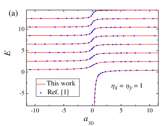
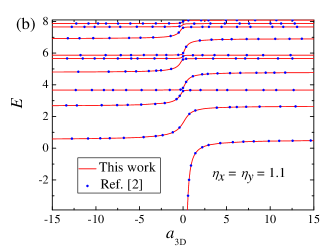
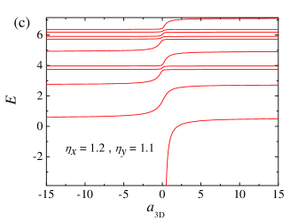
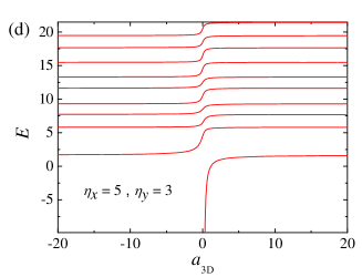
Figure 1: (color online) The energy spectrum of the relative motion of two atoms in a 3D harmonic trap with aspect rations $(\eta_{x}=\eta_{y}=1)$ (a), $(\eta_{x}=\eta_{y}=1.1)$ (b), $(\eta_{x}=1.2,\eta_{y}=1.1)$ (c) and $(\eta_{x}=5,\eta_{y}=3)$ (d). We show the results given by Eq. (1) and the expression (39) of function $J_{\rm 3D}(E)$ with solid lines. In (a) and (b) we also show the results given by Refs. Busch et al. (1998) and Idziaszek and Calarco (2005) with blue dots, respectively. Here we use the natural unit $\hbar=2\mu=\omega_{z}=1$.

II.3 Energy Spectrum

By solving Eq. (13) with the expression (39) of $J_{\rm 3D}(E)$, we can derive the complete eigen-energy spectrum of the complete Hamiltonian $\hat{H}$ of the two-atom relative motion. In Fig. 1(a-d) we show the energy spectrum of the relative motion of two atoms in 3D harmonic traps with various aspect ratios $\eta_{x,y}$, which is derived via Eqs. (13, 39). In Fig. 1(a) and (b) we consider the traps with spherical symmetry ($\eta_{x}=\eta_{y}=1$) and axial symmetry ($\eta_{x}=\eta_{y}=1.1$), respectively, and show that the results given by our approach are same as the ones from the methods in Refs. Busch et al. (1998) and Idziaszek and Calarco (2005). In Fig. 1(c) and (d) we show the results for 3D completely anisotropic traps whose frequencies in every direction are similar ($\eta_{x}=1.2,\eta_{y}=1.1$) and quite different ($\eta_{x}=5,\eta_{y}=3$) with each other, respectively.

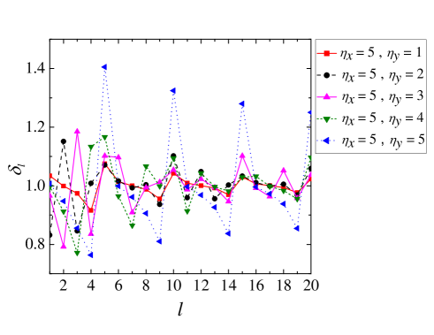
Figure 2: (color online) The normalized energy spacing $\delta_{l}$ defined in Eq. (47) for the lowest 20 excited states of the systems with $a_{{\rm 3D}}=\infty$, $\eta_{x}=5$ and $\eta_{y}$ ($\eta_{y}=1,2,3,4,5$). Here we also use the natural unit $\hbar=2\mu=\omega_{z}=1$

As an example of the application of our method, we make a simple investigation for the energy-level distribution for the systems with integer aspect ratios $\eta_{x}$ and $\eta_{y}$. This property is crucial for many important problems such as thermalization and quantum chaotic behaviors. It is clear that for non-interacting cases (i.e., for $a_{{\rm 3D}}=0$) the energy levels of these systems are distributed with equal spacing. However, when $a_{{\rm 3D}}\neq 0$ the energy-level distributions become uneven, i.e., the energy spacings become unequal with each other. Nevertheless, for systems with different aspect ratios, the “degree of unevenness” of the energy-level distributions, or the fluctuation of the energy spacings, are quite different. In Ref. Idziaszek and Calarco (2005) it was found that for the pancake-shape traps with $\eta_{x}\gg 1$ and $\eta_{y}=1$, the energies are almost distributed with equal spacing (i.e., the level spacings are almost equal), while for the cigar-shape traps with $\eta_{x}=\eta_{y}\gg 1$ the eigen-energies are distributed very even (i.e., the energy spacings fluctuates significantly). Here we study the intermediate cases between the “pancake limit” and the “cigar limit”, i.e., the systems with $a_{{\rm 3D}}=\infty$, $\eta_{x}=5$ and various values of $\eta_{y}$ ($\eta_{y}=1,2,3,4,5$). We define $\Delta_{l}$ ($l=1,2,3,...;\Delta_{l}>0$) as the spacing between the $l$-th and $(l+1)$-th excited-state energy of our systems, and calculate the “normalized” energy spacing

$$\delta_{l}\equiv\frac{\Delta_{l}}{\frac{1}{20}\sum_{l=1}^{20}\Delta_{l}},\ \ \ (l=1,...,20)$$ (47)

for the lowest 20 excited states for each system. As shown in Fig. 2, when the system is crossed from the pancake-shape limit to the cigar-shape, i.e., $\eta_{y}$ is increased from $1$ to $5$, the fluctuation of $\delta_{l}$ monotonically increases, i.e., the energy-level distribution becomes more and more uneven. In future works we will perform more systematic investigations for the energy-level distribution of two ultracold atoms in a completely anisotropic harmonic trap.

II.4 Eigen-State of $\hat{H}$

Furthermore, Eqs. (11) and (12) yields that for a given eigen-energy $E$ of the total Hamiltonian $\hat{H}$ for the two-atom relative motion, the corresponding the eigen-state $|\Psi\rangle$ satisfies

$$\langle{\bf r}|\Psi\rangle \propto \langle{\bf r}|\frac{1}{E-\hat{H}_{0}}|{\bf 0}\rangle=\sum_{\bf n}\frac{\langle{\bf r}|{\bf n}\rangle\langle{\bf n}|{\bf 0}\rangle}{E-E_{\bf n}}.$$ (48)

Thus, considering the normalization condition $\langle\Psi|\Psi\rangle=1$, we obtain the expression for wave function of the eigen-state:

$$\langle{\bf r}|\Psi\rangle=\frac{1}{\sqrt{\sum_{{\bf n}}\left|c_{{\bf n}}\right|^{2}}}\sum_{\bf n}c_{\bf n}\phi_{n_{x}}(\eta_{x},x)\phi_{n_{y}}(\eta_{y},y)\phi_{n_{z}}(\eta_{z},z),$$

(49)

with

$$c_{{\bf n}}=\frac{1}{(E-E_{{\bf n}})}\phi_{n_{x}}(\eta_{x},0)\phi_{n_{y}}(\eta_{y},0)\phi_{n_{z}}(\eta_{z},0).$$ (50)

Here $(x,y,z)$ are the components of ${\bf r}$, the function $\phi_{n}(\eta,X)$ is defined in Eq. (72). It is just the eigen wave function of a one-dimensional harmonic oscillator and satisfies $\langle{\bf r}|{\bf n}\rangle=\phi_{n_{x}}(\eta_{x},x)\phi_{n_{y}}(\eta_{y},y)\phi_{n_{z}}(\eta_{z},z)$. Using Eqs. (68, 69) one can easily derive the normalized eigen-state $|\Psi\rangle$ of $\hat{H}$ from the eigen-energy $E$ Busch et al. (1998); Idziaszek and Calarco (2006); Guan et al. (2019).

III 2D Systems

Now we consider two atoms confined in a 2D anisotropic harmonic trap in the $x-z$ plane. As above, here we assume the trapping frequencies $\omega_{x}$ ($\omega_{z}$) in the $x(z)$-direction are same for each atom. Thus, by separating out the CoM degree of freedom, we can obtain the free Hamiltoian operator for the relative motion. In our natural unit with $\hbar=2\mu=\omega_{z}=1$ this free Hamiltonian can be expressed as

$$\hat{H}_{0}^{\rm(2D)}=\hat{{\bf p}}_{\rm 2D}^{2}+\frac{1}{4}\left(\eta_{x}\hat{x}^{2}+\hat{z}^{2}\right),$$ (51)

where $\eta_{x}=\omega_{x}/\omega_{z}$ is the aspect ratio, as in Sec. II. In Eq. (51), $\hat{{\bf p}}_{\rm 2D}$ and $\hat{\bm{\rho}}\equiv(\hat{x},\hat{z})$ are the relative momentum and coordinate operators, respectively. We further assume that the two atoms experience a 2D $s$-wave zero-range interaction with 2D scattering length $a_{{\rm 2D}}$, and model this potential with the 2D Bethe-Perierls boundary condition (BPC). Explicitly, in our calculation the eigen-energy $E$ and corresponding eigen-state $|\Psi\rangle$ for these two interacting atoms should satisfy the equation

$$\langle\bm{\rho}|\hat{H}_{0}^{\rm(2D)}|\Psi\rangle=E\langle\bm{\rho}|\Psi\rangle;\ \ {\rm for}\ \rho>0,$$ (52)

and the BPC Verhaar et al. (1984)

$$\lim_{\rho\rightarrow 0}\langle\bm{\rho}|\Psi\rangle\propto\left(\ln\rho-\ln a_{{\rm 2D}}\right),$$ (53)

where $|\bm{\rho}\rangle$ is the eigen-state of the relative-coordinate operator $\hat{\bm{\rho}}$, with the corresponding eigen-energy $\bm{\rho}$, and $\rho=|\bm{\rho}|$. Namely, the wave function $\langle\bm{\rho}|\Psi\rangle$ satisfies the eigen-equaiton of the free Hamiltonian $\hat{H}_{0}^{\rm(2D)}$ in the region other than the origin (i.e., the region with $\rho>0$), and has the singular behavior (53) in the limit $\rho\rightarrow 0$, which describes the interaction effect. As in the 3D cases, this zero-rang interaction only acts on the states in the subspace with even-parity with respect to the spatial inversion ${\bm{\rho}}\rightarrow-{\bm{\rho}}$, and thus in this work we only consider the eigen-energies in this subspace. In addition, in the long-range limit $\rho\rightarrow\infty$ the wave function $\langle\bm{\rho}|\Psi\rangle$ should satisfy

$$\lim_{\rho\rightarrow\infty}\langle\bm{\rho}|\Psi\rangle=0.$$ (54)

III.1 Expression of $J_{\rm 2D}(E)$

The solution to Eq. (52) and the long-range condition (54) is proportional to the 2D Green’s function, i.e.,

$$\langle\bm{\rho}|\Psi\rangle\propto G_{0}^{\rm(2D)}(E;{\bf\bm{\rho}})\equiv\langle{\bf\bm{\rho}}|\frac{1}{E-\hat{H}_{0}^{\rm(2D)}}|{\bf 0}\rangle.$$ (55)

Therefore, we can derive the algebrac equation for the eigen-energy $E$ by matching $G_{0}^{\rm(2D)}(E;{\bf\bm{\rho}})$ with the BPC (53). To this end we need to expand $G_{0}^{\rm(2D)}(E;{\bf\bm{\rho}})$ in the limit $\rho\rightarrow 0$. This expansion can be done with the similar approach as in Sec. II, and we show the detail in Appendix C. Finally we obtain

$$\lim_{\rho\rightarrow 0}G_{0}^{\rm(2D)}(E;{\bf\bm{\rho}})=\frac{1}{2\pi}\ln\rho-2\left[W_{\rm 2D}(E)+\int_{0}^{+\infty}I_{\rm 2D}(E,\beta)d\beta\right],$$ (56)

where the functions $W_{\rm 2D}(E)$ and $I_{\rm 2D}(E,\beta)$ being defined as

$$W_{\rm 2D}(E)=\frac{\sqrt{\eta_{x}}}{2}\sum_{n_{x}\in C_{E}^{\rm(2D)}}\left\{\frac{\Gamma\left[\frac{1}{4}-\frac{\left(E-\epsilon_{n_{x}}\right)}{2}\right]2^{n_{x}-2}}{\Gamma\left(\frac{1-n_{x}}{2}\right)^{2}\Gamma(n_{x}+1)\Gamma\left[\frac{3}{4}-\frac{\left(E-\epsilon_{n_{x}}\right)}{2}\right]}\right\}-\frac{\gamma}{4\pi}-\frac{1}{8\pi}\ln\left(\frac{\kappa}{4}\right),$$ (57)

and

$$I_{\rm 2D}(E,\beta) = \frac{e^{\beta E}}{2}\prod_{\alpha=x,z}\sqrt{\frac{\eta_{\alpha}}{4\pi\sinh\left(\eta_{\alpha}\beta\right)}}-\frac{1}{8\pi\beta}e^{-\kappa\beta}-\sqrt{\frac{\eta_{x}}{4\sinh\beta}}\sum_{n_{x}\in C_{E}^{\rm(2D)}}\left\{\frac{2^{n_{x}-\frac{3}{2}}}{\Gamma\left(\frac{1-n_{x}}{2}\right)^{2}\Gamma(n_{x}+1)}e^{\beta(E-\epsilon_{n_{x}})}\right\},$$ (58)

respectively, in our natural unit. Here $\gamma=0.5772...$ is the Euler’s constant, $\eta_{z}=1$, $\epsilon_{n_{x}}=(n_{x}+1/2)\eta_{x}$, the parameter $\kappa$ could be any positive number and the result is independent of the value of $\kappa$. In Eq. (58) $C_{E}^{\rm(2D)}$ is a number set defined as

$$C_{E}^{\rm(2D)}:\left\{\left.n_{x}\right|n_{x}=0,2,4,6,...;\ \epsilon_{n_{x}}+\frac{1}{2}\leq E\right\}.$$ (59)

Clearly, for $E<E_{0}$ the set $C_{E}^{\rm(2D)}$ is empty and the summation $\sum_{n_{x}\in C_{E}^{\rm(2D)}}$ in the expressions (57, 58) of $W_{\rm 2D}$ and $I_{\rm 2D}$ becomes zero.

Combining Eq. (98), Eq. (55) and Eq. (53), we obtain the equation for the eigen-energy $E$ of our 2D system, which has the form of Eq. (2):

$$J_{{\rm 2D}}(E)=\ln a_{{\rm 2D}}.$$ (60)

Here the function $J_{{\rm 2D}}(E)$ is given by

$$J_{{\rm 2D}}(E)=4\pi\left[W_{\rm 2D}(E)+\int_{0}^{+\infty}I_{\rm 2D}(E,\beta)d\beta\right],$$ (61)

with $W_{\rm 2D}(E)$ and $I_{\rm 2D}(E,\beta)$ being defined in Eq. (57) and Eq. (58), respectively. One can derive the eigen-energies of the relative motion of these two atoms by solving Eq. (60), and further obtain the corresponding eigen-states.

As in the 3D cases, the summations in Eq. (57, 58) are done for finite terms, and the integration in Eq. (61) converges. Therefore, using Eqs. (61, 57, 58) one can efficiently calculate $J_{{\rm 2D}}(E)$. In addition, for the systems with a 2D isotropic trap ($\omega_{x}=\omega_{z}$ or $\eta_{x}=1$), the equaiton (60) for the eigen-energy and the expression (61) for the function $J_{\rm 2D}(E)$ are equivalent to the results derived by Ref. Busch et al. (1998). Explicitly, we have aa (2)

$$J_{\rm 2D}(E)=\frac{d}{dz}\ln\left[\Gamma(z)\right]\Big{|}_{z=\frac{1-E}{2}}-\gamma+\frac{1}{2}\ln 2,\ \ ({\rm for}\ \omega_{x}=\omega_{z}).$$ (62)

III.2 Techniques for Fast Calculation of $J_{{\rm 2D}}(E)$

The techniques shown in Sec. II.B for the fast calculation of $J_{{\rm 3D}}(E)$ can also be directly generalized to the 2D case (Appendix D). In particular, as proved in Appendix D, $J_{\rm 2D}(E)$ given by Eq. (61) can be re-expressed as

$$J_{{\rm 2D}}(E) = 4\pi\left[\int_{0}^{\Lambda}A_{{\rm 2D}}(E,\beta)d\beta+B^{(1)}_{\rm 2D}(E,\Lambda)+B^{(2)}_{\rm 2D}(E,\Lambda)-\frac{\Gamma(0,\kappa\Lambda)}{8\pi}\right],$$ (63)

where $\Lambda$ and $\kappa$ are arbitrary finite positive numbers, as in Eqs. (57, 58, 40), $\Gamma[a,z]$ is the incomplete Gamma function and the functions $A_{{\rm 2D}}(E,\beta)$ and $B^{(1,2)}_{{\rm 2D}}(E,\Lambda)$ are defined as

$$A_{{\rm 2D}}(E,\beta) = \frac{e^{\beta E}}{2}\prod_{\alpha=x,z}\sqrt{\frac{\eta_{\alpha}}{4\pi\sinh\left(\eta_{\alpha}\beta\right)}}-\frac{1}{8\pi\beta}e^{-\kappa\beta};$$ (64)

$$B^{(1)}_{{\rm 2D}}(E,\Lambda) = -\frac{\gamma}{4\pi}-\frac{1}{8\pi}\ln\left(\frac{\kappa}{4}\right)+\sum_{n_{x}\in C_{E}^{{\rm(2D)}}}\left\{\frac{\sqrt{\eta_{x}}2^{n_{x}-3}e^{(E-\epsilon_{n_{x}}-{3\over 2})\Lambda}\sqrt{e^{2\Lambda}-1}\cdot\Gamma\left({1\over 4}-{{E-\epsilon_{n_{x}}}\over 2}\right)}{\Gamma\left(\frac{1-n_{x}}{2}\right)^{2}\Gamma(n_{x}+1)\Gamma\left({5\over 4}-{{E-\epsilon_{n_{x}}}\over 2}\right)}\right.$$ (66)

$$\ \ \ \ \ \ \ \ \ \ \ \ \ \ \ \ \ \ \ \ \ \ \ \ \ \ \ \ \ \ \ \ \ \ \ \ \ \ \ \ \ \ \left.\times_{2}F^{1}\quantity[1,\frac{3}{4}-\frac{E-\epsilon_{n_{x}}}{2},\frac{5}{4}-\frac{E-\epsilon_{n_{x}}}{2},e^{-2\Lambda}]\begin{array}[]{c}\vspace{10pt}\hfil\end{array}\right\};$$

and

$$B^{(2)}_{{\rm 2D}}(E,\Lambda) = -\sum_{n_{x}\notin C_{E}^{{\rm(2D)}}}\frac{2^{n_{x}-\frac{3}{2}}\cdot\sqrt{\eta_{x}\csch{\Lambda}}}{\Gamma\left(\frac{1-n_{x}}{2}\right)^{2}\Gamma(n_{x}+1)}\cdot\frac{e^{(E-\epsilon_{n_{x}}-2)\Lambda}(e^{2\Lambda}-1)\times_{2}\!F^{1}\quantity[1,\frac{3}{4}-\frac{E-\epsilon_{n_{x}}}{2},\frac{5}{4}-\frac{E-\epsilon_{n_{x}}}{2},e^{-2\Lambda}]}{2\quantity(E-\epsilon_{n_{x}})-1},$$

(67)

respectively, with ${}_{2}F^{1}$ being the Hypergeomtric function. As in the 3D cases, the expression (63) of $J_{\rm 2D}(E)$ has the advantages (A) and (B) shown in Sec. II. B. Therefore, the numerical calculations based on Eq. (63) is quite possibly to be faster then the one based on Eq. (61), especially for the high-energy cases with large $E$.

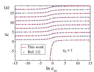
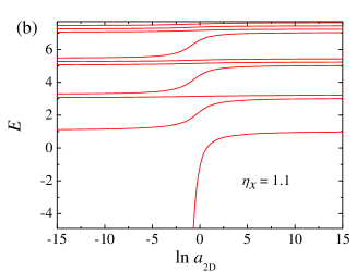
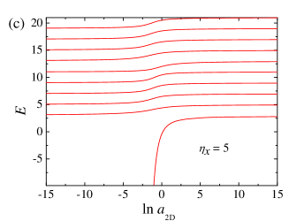
Figure 3: (color online) The energy spectrum of the relative motion of two atoms in a 2D harmonic trap with $\eta_{x}=1$ (a), $\eta_{x}=1.1$ (b) and $\eta_{x}=5$ (c). We show the results given by Eq. (2) and the expression (61) of the function $J_{\rm 2D}(E)$ with solid lines. In (a) we also show the results given by Ref. Busch et al. (1998) with blue dots. Here we use the natural unit $\hbar=2\mu=\omega_{z}=1$.

III.3 Energy Sepectrum and Eigen-States

In Fig. 3 (a) we illustrate the energy spectrum for the cases with an isotropic 2D trap ($\eta_{x}=1$), and show that our results are same as the ones from Ref. Busch et al. (1998). In Fig. 3 (b) and (c) we show the results for anisotropic 2D traps which have similar ($\eta_{x}=1.1$) and quite different ($\eta_{x}=5$) frequencies in the $x$- and $z$-directions.

In addition, similar to Sec. II.D, one can also derive the corresponding eigen-state $|\Psi\rangle$ with eigen-energy $E$, which satisfies Eq. (52) and the boundary conditions (53, 54), as well as the normalization condition $\langle\Psi|\Psi\rangle=1$. With Eq. (55) and the similar approach as in Sec. II. D we obtain

$$\langle{\bm{\rho}}|\Psi\rangle=\frac{1}{\sqrt{\sum_{\bf m}\left|d_{{\bf m}}\right|^{2}}}\sum_{\bf m}d_{\bf m}\phi_{m_{x}}(\eta_{x},x)\phi_{m_{z}}(1,z),$$

(68)

with

$$d_{{\bf m}}=\frac{1}{\left(E-E^{\rm(2D)}_{{\bf m}}\right)}\phi_{m_{x}}(\eta_{x},0)\phi_{m_{z}}(1,0).$$ (69)

Here $(x,z)$ are the components of ${\bm{\rho}}$, ${\bf m}=(m_{x},m_{y})$ with $m_{x,y}=0,1,2,...$, $E^{\rm(2D)}_{{\bf m}}=(m_{x}+1/2)\eta_{x}+(m_{z}+1/2)$, and the function $\phi_{n}(\eta,X)$ is defined in Eq. (72).

IV generalization of our approach to other problems

At the end of this work, we briefly summarize the main ideas of our approach used in the above calculations, and discuss how to generalize these ideas. Here we take the 3D systems as an example.

The key step for solving the two-body problem with zero-rang interaction is the calculation of the free Green’s operator ${\hat{G}}_{0}(E)\equiv 1/[E-\hat{H}_{0}]$. When $E$ is less than the ground-state energy $E_{0}$ of $\hat{H}_{0}$, ${\hat{G}}_{0}(E)$ can be directly expressed as the Laplace transform of of the imaginary-time evolution operator $e^{-\beta\hat{H}_{0}}$, i.e., we have ${\hat{G}}_{0}(E)=-\int_{0}^{+\infty}e^{\beta(E-\hat{H}_{0})}d\beta$. However, when $E>E_{0}$ this integration diverges. To solve this problem, we separate ${\hat{G}}_{0}(E)$ into two parts, i.e., the contributions from the high-energy states with ${\bf n}\in U_{E}$ and the ones from the low-energy states with ${\bf n}\in L_{E}$, as shown in Eq. (28). Furthermore, as shown in Eqs. (29, 30), the first part can still be expressed as the Laplace transform of the operator $e^{-\beta\hat{H}_{0}^{{\rm(3D)}}}-\sum_{{\bf n}\in L_{E}}|{\bf n}\rangle\langle{\bf n}|e^{-\beta\left(E_{{\bf n}}\right)}$, which converges for for any non-zero $z$, and the second part only includes finite terms.

It is pointed out that, the definitions of the sets $L_{E}$ and $U_{E}$ are not unique. The only requirements are:

• : $L_{E}$ is the complement of $U_{E}$.

• : $E_{{\bf n}}>E$ for $\forall{\bf n}\in U_{E}$. Namely, the set $L_{E}$ includes (but is not limited to) all ${\bf n}$ which satisfies $E_{{\bf n}}<E$.

For instance, an alternative definition of these two sets is: $U_{E}:\{{\bf n}|E_{{\bf n}}>E\}$ and $L_{E}:\{{\bf n}|E_{{\bf n}}\leq E\}$.

Using this method we can derive the helpful expression (31) of Green’s function $G^{(0)}(E,z{\bf e}_{z})$, which is just the matrix element $\langle z{\bf e}_{z}|{\hat{G}}_{0}(E)|{\bf 0}\rangle$ of the free Green’s operator ${\hat{G}}_{0}(E)$. In this expression there is just a summation for finite terms and a one-dimensional integration $\int_{0}^{+\infty}d\beta\left[K(z;E,\beta)-F(z;E,\beta)\right]$ which converges for any finite $z$.

To complete the calculation we still require to remove the divergent term of the above integration in the limit $z\rightarrow 0$. This divergent term is contributed by the leading term $e^{-\frac{z^{2}}{4\beta}}/(4\pi\beta)^{\frac{3}{2}}$ of the integrand $K(z;E,\beta)-F(z;E,\beta)$ in the limit $\beta\rightarrow 0^{+}$. Therefore, we can remove it via the technique used in Eqs. (18, 19, LABEL:gexpa).

Our above approach for the calculation of the two-body free Green’s function can be directly generalized to other few-body problems of ultracold atoms, especially the ones where the analytical expressions of the eigen-states and imaginary-time propagator of the free Hamiltonian are known, e.g., the few-body problems in mixed-dimensional systems Nishida and Tan (2008). Here we emphasize that, with the help of the Laplace transformation for imaginary-time propagator, the free Green’s operator can always be expressed as a one-dimensional integration, no matter how many degrees of freedoms are involved in the system. Thus, the free Green’s function given by our method always includes a converged one-dimensional integration and summations for finite terms.

V Summary

In this work we derive the algebraic equations for the eigen-energies of two atoms in a 2D or 3D harmonic trap. Our results is applicable for general cases, no matter if the trap is completely anisotropic or has spherical or axial symmetry. Using our results one can easily derive the complete energy spectrum, which can be used for the further theoretical or experimental studies of dynamical or thermodynamical problems. Our approach can be used in other few-body problems of confined ultracold atoms.

Note added: When we finished this work, we realized that recently there is a related work Bougas et al. . The authors derived the expression of $J_{\rm 2D}(E)$ for $E<E_{0}$, and a recurrence relation of $J_{\rm 2D}(E)$ for arbitrary $E$. With this recurrence relation they also obtained the complete energy spectrum of two atoms in a 2D anisotropic confinement, as well as the eigen-states.

Appendix A Proof of Eqs. (36) and (37)

In this appendix we prove Eqs. (36) and (37) in Sec. II.A. To this end, we first show some results on 1D harmonic oscillator, which will be used in our calculation.

A.1 Some properties of 1D harmonic oscillator

Let us consider a 1D harmonic oscillator with frequency $\eta$ and mass $\mu$. The Hamiltonian of this oscillator is ($\hbar=2\mu=1$)

$${\hat{H}}_{\rm ho}={\hat{P}}^{2}+\frac{\eta^{2}{\hat{X}}^{2}}{4},$$ (70)

with ${\hat{X}}$ and ${\hat{P}}$ being the coordinate and momentum operator, respectively. The eigen-energy of ${\hat{H}}_{\rm ho}$ is

$$E_{n}=\left(n+\frac{1}{2}\right)\eta;\ \ \ (n=0,1,2,...),$$ (71)

and the wave function of the eigen-state $|n\rangle$ corresponding to $E_{n}$ can be expressed as

$$\langle X|n\rangle\equiv\phi_{n}(\eta,X)=\left(\frac{\eta}{2\pi}\right)^{\frac{1}{4}}\frac{e^{-\frac{\eta X^{2}}{4}}}{\sqrt{2^{n}\Gamma(n+1)}}H_{n}\left(\sqrt{\frac{\eta}{2}}X\right),$$ (72)

with $|X\rangle$ being the eigen-state of the position operator ${\hat{X}}$ with eigen-value $X$, $H_{n}(X)$ and $\Gamma(\alpha)$ being the Hermitian polynomial and the Gamma function, respectively. The wave function $\phi_{n}(\eta,X)$ also satisfies

$$\langle X|e^{-\beta{\hat{H}}_{\rm ho}}|0\rangle=\sum_{n=0}^{+\infty}\phi_{n}(\eta,X)\phi_{n}^{\ast}(\eta,0)e^{-\beta(n+1/2)\eta}=\sqrt{\frac{\eta}{4\pi\sinh(\eta\beta)}}\exp\left[-\frac{\eta X^{2}\coth{(\eta\beta)}}{4}\right]$$ (73)

for $\beta>0$.

Now we consider the Green’s function $g(\xi;\eta;X)$ of the 1D harmonic oscillator, which is defined as

$$g(\xi;\eta;X)\equiv\langle X|\frac{1}{\xi-{\hat{H}}_{\rm ho}}|0\rangle=\sum_{n=0}^{+\infty}\frac{\phi_{n}(\eta,X)\phi_{n}^{\ast}(\eta,0)}{\xi-E_{n}}.$$ (74)

This function satisfies the differential equation

$$\xi\cdot g(\xi;\eta;X)+\frac{d^{2}}{dX^{2}}g(\xi;\eta;X)-\frac{\eta^{2}X^{2}}{4}g(\xi;\eta;X)=\delta(X)$$ (75)

and the boundary condition

$$\lim_{|X|\rightarrow\infty}g(\xi;\eta;X)=0.$$ (76)

To derive $g(\xi;\eta;X)$, we can first solve the equation (75) in the regions $X>0$ and $X<0$ with the boundary condition (76), and then match the solution with the connection condition at $X=0$, which is given by the term $\delta(X)$ in Eq. (75). With this approach we obtain

$$g(\xi;\eta;X)=\sum_{n=0}^{+\infty}\frac{\phi_{n}(\eta,X)\phi_{n}^{\ast}(\eta,0)}{\xi-E_{n}}=-\frac{\Gamma(\frac{1}{4}-\frac{\xi}{2\eta})}{2^{\frac{5}{4}+\frac{\xi}{2\eta}}\sqrt{\pi\eta}}D_{\frac{\xi-\eta/2}{\eta}}\left(\sqrt{\eta}X\right),$$ (77)

where $D_{\lambda}(\alpha)$ is the parabolic cylinder function. Eq. (77) and the property of the parabolic cylinder function further yields

$$g(\xi;\eta;0)=\sum_{n=0}^{+\infty}\frac{|\phi_{n}(\eta,0)|^{2}}{\xi-(n+1/2)\eta}{=-\frac{\Gamma(\frac{1}{4}-\frac{\xi}{2\eta})}{2\sqrt{2\eta}\Gamma(\frac{3}{4}-\frac{\xi}{2\eta})}.}$$ (78)

A.2 Proof of the two equations

Now we prove Eq. (36) and Eq. (37) in our main text, which are about the expressions of the functions $W_{{\rm 3D}}(E)$ and $I_{{\rm 3D}}(E,\beta)$, respectively. As shown in Sec. II.A, these two functions are defined as

$$W_{{\rm 3D}}(E)\equiv Q(0,E,\beta),$$ (79)

and

$$I_{{\rm 3D}}(E,\beta)\equiv-\tilde{K}(0;E,\beta)+F(0;E,\beta),$$ (80)

with the functions $Q(z,E,\beta)$, $\tilde{K}(z;E,\beta)$ defined in Eq. (32) and Eq. (19), respectively. Thus, we have

$$Q(0;E,\beta) = \sum_{{\bf n}\in L_{E}}\frac{\langle{\bf 0}|{\bf n}\rangle\langle{\bf n}|{\bf 0}\rangle}{E-E_{{\bf n}}};$$ (81)

$$F(0;E,\beta) = \sum_{{\bf n}\in L_{E}}\langle{\bf 0}|{\bf n}\rangle\langle{\bf n}|{\bf 0}\rangle e^{-\beta\left(E_{{\bf n}}-E\right)}.$$ (82)

It is clear that the eigen-state $|{\bf n}\rangle$ of the 3D free Hamiltonian ${\hat{H}}_{0}$, which is defined in Sec. II.A, satisfies $\langle{\bf 0}|{\bf n}\rangle=0$ when $n_{x}$ or $n_{y}$ is odd. Using this fact and the definitions of the sets $L_{E}$ and $C_{E}^{\rm(3D)}$, which are given in Eqs. (25, 38) of our main text, we obtain

$$Q(0;E,\beta) = \sum_{(n_{x},n_{y})\in C_{E}^{\rm(3D)}}\sum_{n_{z}=0}^{+\infty}\frac{\langle{\bf 0}|{\bf n}\rangle\langle{\bf n}|{\bf 0}\rangle}{E-E_{{\bf n}}}$$ (83)

$$=\sum_{(n_{x},n_{y})\in C_{E}^{\rm(3D)}}\left\{|\phi_{n_{x}}(\eta_{x},0)|^{2}|\phi_{n_{y}}(\eta_{y},0)|^{2}\left[\sum_{n_{z}=0}^{+\infty}\frac{|\phi_{n_{z}}(\eta_{z},0)|^{2}}{\left(E-\epsilon_{n_{x}}-\epsilon_{n_{y}}\right)-\epsilon_{n_{z}}}\right]\right\},$$

and

$$F(0;E,\beta) = \sum_{(n_{x},n_{y})\in C_{E}^{\rm(3D)}}\sum_{n_{z}=0}^{+\infty}\langle{\bf 0}|{\bf n}\rangle\langle{\bf n}|{\bf 0}\rangle e^{-\beta\left(E_{{\bf n}}-E\right)}$$ (84)

$$=\sum_{(n_{x},n_{y})\in C_{E}^{\rm(3D)}}\left\{|\phi_{n_{x}}(\eta_{x},0)|^{2}|\phi_{n_{y}}(\eta_{y},0)|^{2}e^{\beta(E-\epsilon_{n_{x}}-\epsilon_{n_{y}})}\left[\sum_{n_{z}=0}^{+\infty}|\phi_{n_{z}}(\eta_{z},0)|^{2}e^{-\beta\epsilon_{n_{z}}}\right]\right\},$$

where $\eta_{x,y,z}$ and $\epsilon_{n_{x,y,z}}$ are defined in Sec. II, and the function $\phi_{n}(\eta,X)$ is defined in Eq. (72).

Substituting Eq. (78) into Eq. (83) and then into Eq. (79), and using the property

$$H_{n}(0)=\frac{2^{n}\sqrt{\pi}}{\Gamma(\frac{1-n}{2})}$$ (85)

of the Hermitian polynomial, we can derive Eq. (36). Moreover, Substituting Eq. (73) into Eq. (84) and then into Eq. (80), and using Eqs. (85), (19) and (LABEL:kr), we can derive Eq. (37).

Appendix B Proof of Eq. (40)

In this appendix we prove Eq. (40) in Sec. II.B. To this end, we separate the integration in Eq. (39) into two parts, i.e.,

$$\int_{0}^{\infty}I_{{\rm 3D}}(E,\beta)d\beta=\int_{0}^{\Lambda}I_{{\rm 3D}}(E,\beta)d\beta+\int_{\Lambda}^{\infty}I_{{\rm 3D}}(E,\beta)d\beta,$$ (86)

with $\Lambda$ being an arbitrary finite positive number. In addition, using the definition (37) of $I_{{\rm 3D}}(E,\beta)$, we immediately obtain

$$\int_{0}^{\Lambda}I_{{\rm 3D}}(E,\beta)d\beta$$

$$= \int_{0}^{\Lambda}A_{{\rm 3D}}(E,\beta)d\beta+\sum_{(n_{x},n_{y})\in C_{E}^{{\rm(3D)}}}\int_{0}^{\Lambda}\frac{2^{n_{x}+n_{y}-2}\sqrt{\pi\eta_{x}\eta_{y}}\ e^{\beta(E-\epsilon_{n_{x}}-\epsilon_{n_{y}})}}{\Gamma\left(\frac{1-n_{x}}{2}\right)^{2}\Gamma\left(\frac{1-n_{y}}{2}\right)^{2}\Gamma(n_{x}+1)\Gamma(n_{y}+1)\sqrt{\sinh\beta}}d\beta$$

$$= \int_{0}^{\Lambda}A_{{\rm 3D}}(E,\beta)d\beta$$

$$+\sum_{(n_{x},n_{y})\in C_{E}^{{\rm(3D)}}}\frac{2^{n_{x}+n_{y}-{5\over 2}}\sqrt{\pi\eta_{x}\eta_{y}}}{\Gamma\left(\frac{1-n_{x}}{2}\right)^{2}\Gamma\left(\frac{1-n_{y}}{2}\right)^{2}\Gamma(n_{x}+1)\Gamma(n_{y}+1)}\Bigg{\{}{\sqrt{\pi}\Gamma\left({1\over 4}-{{E-\epsilon_{n_{x}}-\epsilon_{n_{y}}}\over 2}\right)\over\Gamma\left({3\over 4}-{{E-\epsilon_{n_{x}}-\epsilon_{n_{y}}}\over 2}\right)}-$$

$$\ \ \ \ \ \ \ \ \ \ \ \ \ \ \ \ \ \ \ \frac{\Gamma\left({1\over 4}-{{E-\epsilon_{n_{x}}-\epsilon_{n_{y}}}\over 2}\right)}{\Gamma\left({5\over 4}-{{E-\epsilon_{n_{x}}-\epsilon_{n_{y}}}\over 2}\right)}e^{(E-\epsilon_{n_{x}}-\epsilon_{n_{y}}-{3\over 2})\Lambda}\sqrt{e^{2\Lambda}-1}\times_{2}\!F^{1}\quantity[1,\frac{3}{4}-\frac{E-\epsilon_{n_{x}}-\epsilon_{n_{y}}}{2},\frac{5}{4}-\frac{E-\epsilon_{n_{x}}-\epsilon_{n_{y}}}{2},e^{-2\Lambda}]\Bigg{\}}$$ (87)

with $A_{{\rm 3D}}(E,\beta)$ being defined in Eq. (41).

Now we calculate the term $\int_{\Lambda}^{\infty}I_{{\rm 3D}}(E,\beta)d\beta$ in Eq. (86). We first notice that, according to Eqs. (80,84,19,LABEL:kr), $I_{{\rm 3D}}(E,\beta)$ can be re-expressed as

$$I_{{\rm 3D}}(E,\beta) = \left(\frac{1}{4\pi\beta}\right)^{\frac{3}{2}}-\sum_{n_{x},n_{y},n_{z}}\langle{\bf 0}|{\bf n}\rangle\langle{\bf n}|{\bf 0}\rangle e^{-\beta\left(E_{{\bf n}}-E\right)}+\sum_{(n_{x},n_{y})\in C_{E}^{\rm(3D)}}\sum_{n_{z}=0}^{+\infty}\langle{\bf 0}|{\bf n}\rangle\langle{\bf n}|{\bf 0}\rangle e^{-\beta\left(E_{{\bf n}}-E\right)}$$ (88)

$$= \left(\frac{1}{4\pi\beta}\right)^{\frac{3}{2}}-\sum_{(n_{x},n_{y})\notin C_{E}^{\rm(3D)}}\sum_{n_{z}=0}^{+\infty}\langle{\bf 0}|{\bf n}\rangle\langle{\bf n}|{\bf 0}\rangle e^{-\beta\left(E_{{\bf n}}-E\right)}$$

$$= \left(\frac{1}{4\pi\beta}\right)^{\frac{3}{2}}-\sum_{(n_{x},n_{y})\notin C_{E}^{\rm(3D)}}\left\{|\phi_{n_{x}}(\eta_{x},0)|^{2}|\phi_{n_{y}}(\eta_{y},0)|^{2}e^{\beta(E-\epsilon_{n_{x}}-\epsilon_{n_{y}})}\left[\sum_{n_{z}=0}^{+\infty}|\phi_{n_{z}}(\eta_{z},0)|^{2}e^{-\beta\epsilon_{n_{z}}}\right]\right\},$$

where $\epsilon_{n_{x,y,z}}$ is defined in Sec. II, and the function $\phi_{n}(\eta,X)$ is defined in Eq. (72). Moreover, Substituting Eq. (73) and Eq. (85) into Eq. (88), we further obtain

$$I_{{\rm 3D}}(E,\beta) = \left(\frac{1}{4\pi\beta}\right)^{\frac{3}{2}}-\sqrt{\frac{\pi\eta_{x}\eta_{y}}{8\sinh\beta}}\sum_{(n_{x},n_{y})\notin C_{E}^{{\rm(3D)}}}\left\{\frac{2^{n_{x}+n_{y}-\frac{1}{2}}}{\Gamma\left(\frac{1-n_{x}}{2}\right)^{2}\Gamma\left(\frac{1-n_{y}}{2}\right)^{2}\Gamma(n_{x}+1)\Gamma(n_{y}+1)}e^{\beta(E-\epsilon_{n_{x}}-\epsilon_{n_{y}})}\right\},$$ (89)

where $\eta_{x,y,z}$ is defined in Sec. II. Doing the integration $\int_{\Lambda}^{\infty}I_{{\rm 3D}}(E,\beta)d\beta$ in both sides of Eq. (89), we further obtain

$$\int_{\Lambda}^{\infty}I_{{\rm 3D}}(E,\beta)d\beta = B^{(2)}_{\rm 3D}(E,\Lambda)+\quantity(\frac{1}{2\pi})^{3/2}\frac{1}{\sqrt{2\Lambda}},$$ (90)

where $B^{(2)}_{\rm 3D}(E,\Lambda)$ is defined in Eq. (44).

Substituting Eqs. (87, 90) into Eq. (86) and then into Eq. (39), and further using Eqs. (36), we can derive Eq. (40).

Appendix C Proof of Eqs. (57) and (58)

In this appendix we prove Eqs. (57) and (58) in Sec. III, which is related to the behavior of the 2D Green’s function $G_{0}^{\rm(2D)}(E;\bm{\rho})$ in the limit $|{\bm{\rho}}|\rightarrow 0$. Our approach is similar to the method used in Sec. II.A.

As in Sec. II and Appendix A, by choosing ${\bm{\rho}}=\rho{\bf e}_{z}$ ($\rho>0$) and making direct calculations we can find that

$$G_{0}^{\rm(2D)}(E;\rho{\bf e}_{z})=-\int_{0}^{\infty}\left[K_{\rm 2D}(\rho;E,\beta)-Y(\rho;E,\beta)\right]d\beta+Z(\rho;E),$$ (91)

which is similar to the expression (31) of the 3D free Green’s function. Here the functions $K_{\rm 2D}(\rho;E,\beta)$, $Y(\rho;E,\beta)$ and $Z(\rho;E)$ are defined as

$$K_{\rm 2D}(\rho;E,\beta)=e^{\beta E}\langle\rho{\bf e}_{z}|e^{-\beta\hat{H}_{0}^{(2D)}}|\bm{0}\rangle=\left(\prod_{\alpha=x,z}\sqrt{\frac{\eta_{\alpha}}{4\pi\sinh\left(\eta_{\alpha}\beta\right)}}\right)\cdot\exp\left[\beta E-\frac{\operatorname{coth}\left(\beta\right)}{4}\rho^{2}\right];$$ (92)

$$Y(\rho;E,\beta)=\sum_{n_{x}\in C_{E}^{(2D)}}\sum_{n_{z}=0}^{+\infty}e^{\beta\left(E-E_{\bf n}\right)}\langle\rho{\bf e}_{z}|{\bf n}\rangle\langle{\bf n}|{\bf 0}\rangle;$$ (93)

$$Z(\rho;E)=\sum_{n_{x}\in C_{E}^{(2D)}}\sum_{n_{z}=0}^{+\infty}\frac{\langle\rho{\bf e}_{z}|{\bf n}\rangle\langle{\bf n}|{\bf 0}\rangle}{E-E_{\bf n}},$$ (94)

where $\eta_{x,z}$ and $\epsilon_{n_{x,z}}$ have the same definition as in Sec. II and $C_{E}^{(2D)}$ is defined in Eq. (59). Furthermore, the integration in Eq. (95) diverges in the limit $z\rightarrow 0$, and we can remove this divergence via the similar approach as in Sec. III. To this end, we re-express Eq. (95) as

$$G_{0}^{\rm(2D)}(E;\rho{\bf e}_{z})=-\int_{0}^{\infty}\frac{1}{4\pi\beta}\cdot\exp\left(-\beta\kappa-\frac{1}{4\beta}\rho^{2}\right)d\beta-\int_{0}^{\infty}\left[\tilde{K}_{\rm 2D}(\rho;E,\beta)-Y(\rho;E,\beta)\right]d\beta+Z(\rho;E),$$ (95)

with $\kappa$ being any positive number and

$$\tilde{K}_{\rm 2D}(\rho;E,\beta)=K_{\rm 2D}(\rho;E,\beta)-\frac{1}{4\pi\beta}\cdot\exp\left(-\beta\kappa-\frac{1}{4\beta}\rho^{2}\right).$$ (96)

Furthermore, using the result

$$\int_{0}^{\infty}\frac{1}{4\pi\beta}\cdot\exp\left(-\beta\kappa-\frac{1}{4\beta}\rho^{2}\right)d\beta=-\frac{1}{2\pi}\ln\rho-\frac{1}{2\pi}\gamma-\frac{1}{4\pi}\ln\frac{\kappa}{4}+{\cal O}(\rho)\ \ \ ({\rm for}\ \rho>0),$$ (97)

with $\gamma=0.5772...$ being the Euler’s constant, we derive a result with the same form of Eq. (98):

$$\lim_{\rho\rightarrow 0}G_{0}^{\rm(2D)}(E;{\bf\bm{\rho}})=\frac{1}{2\pi}\ln\rho-2\left[W_{\rm 2D}(E)+\int_{0}^{+\infty}I_{\rm 2D}(E,\beta)d\beta\right].$$ (98)

In this step the functions $W_{\rm 2D}(E)$ and $I_{\rm 2D}(E,\beta)$ are given by

$$W_{\rm 2D}(E) = -\frac{1}{4\pi}\gamma-\frac{1}{8\pi}\ln\frac{\kappa}{4}-\frac{1}{2}Z(0,E);$$ (99)

$$I_{\rm 2D}(E,\beta) = \frac{1}{2}\left[\tilde{K}_{\rm 2D}(0;E,\beta)-Y(0;E,\beta)\right].$$ (100)

Moreover, with the method in Appendix A, we can derive the alternative expressions of $W_{\rm 2D}(E)$ and $I_{\rm 2D}(E,\beta)$, i.e., Eqs. (57) and (58).

Appendix D Techniques for fast calculation of $J_{{\rm 2D}}(E)$

In this appendix we generalize the techniques shown in Sec.II.B and Appendix B to the 2D case. We first generalize Eqs. (40-44) to the 2D cases and prove Eq. (63). This can be done via direct calculations with the method shown in Appendix B. We separate the integration in Eq. (61) into two parts, i.e.,

$$\int_{0}^{\infty}I_{{\rm 2D}}(E,\beta)d\beta=\int_{0}^{\Lambda}I_{{\rm 2D}}(E,\beta)d\beta+\int_{\Lambda}^{\infty}I_{{\rm 2D}}(E,\beta)d\beta,$$ (101)

with $\Lambda$ being an arbitrary positive number. In addition, using the definition (58) of $I_{{\rm 2D}}(E,\beta)$, we immediately obtain

$$\int_{0}^{\Lambda}I_{{\rm 2D}}(E,\beta)d\beta$$

$$= \int_{0}^{\Lambda}A_{{\rm 2D}}(E,\beta)d\beta-\sum_{n_{x}\in C_{E}^{{\rm(2D)}}}\int_{0}^{\Lambda}\frac{2^{n_{x}-\frac{5}{2}}\sqrt{\eta_{x}}e^{\beta(E-\epsilon_{n_{x}})}}{\Gamma\left(\frac{1-n_{x}}{2}\right)^{2}\Gamma(n_{x}+1)\sqrt{\sinh\beta}}d\beta$$

$$= \int_{0}^{\Lambda}A_{{\rm 2D}}(E,\beta)d\beta+\sum_{(n_{x})\in C_{E}^{{\rm(2D)}}}\frac{2^{n_{x}-3}\sqrt{\eta_{x}}}{\Gamma\left(\frac{1-n_{x}}{2}\right)^{2}\Gamma(n_{x}+1)}\Bigg{\{}-{\sqrt{\pi}\Gamma\left({1\over 4}-{{E-\epsilon_{n_{x}}}\over 2}\right)\over\Gamma\left({3\over 4}-{{E-\epsilon_{n_{x}}}\over 2}\right)}+$$

$$\frac{\Gamma\left({1\over 4}-{{E-\epsilon_{n_{x}}}\over 2}\right)}{\Gamma\left({5\over 4}-{{E-\epsilon_{n_{x}}}\over 2}\right)}e^{(E-\epsilon_{n_{x}}-{3\over 2})\Lambda}\sqrt{e^{2\Lambda}-1}\times_{2}\!F^{1}\quantity[1,\frac{3}{4}-\frac{E-\epsilon_{n_{x}}}{2},\frac{5}{4}-\frac{E-\epsilon_{n_{x}}}{2},e^{-2\Lambda}]\Bigg{\}}$$ (102)

with $A_{{\rm 2D}}(E,\beta)$ being defined in Eq. (64).

Furthermore, using the method in Appendix B, we find that the function $I_{\rm 2D}(E,\beta)$ defined in Eq. (58) has an alternative expression

$$I_{\rm 2D}(E,\beta) = -\frac{1}{8\pi\beta}e^{-\kappa\beta}+\sqrt{\frac{\eta_{x}}{4\sinh\beta}}\sum_{n_{x}\notin C_{E}^{\rm(2D)}}\left\{\frac{2^{n_{x}-\frac{3}{2}}}{\Gamma\left(\frac{1-n_{x}}{2}\right)^{2}\Gamma(n_{x}+1)}e^{\beta(E-\epsilon_{n_{x}})}\right\},$$ (103)

which is similar to Eq. (89). Thus, doing the integration $\int_{\Lambda}^{\infty}I_{{\rm 2D}}(E,\beta)d\beta$ in both sides of Eq. (103), we further obtain

$$\int_{\Lambda}^{\infty}I_{{\rm 2D}}(E,\beta)d\beta = B^{(2)}_{\rm 2D}(E,\Lambda)-\frac{\Gamma(0,\kappa\Lambda_{2})}{8\pi}$$ (104)

where $\Gamma[a,z]$ is the incomplete Gamma function and $B^{(2)}_{\rm 2D}(E,\Lambda)$ is defined in Eq. (67).

As in Appendix B, substituting Eqs. (102, 104) into Eq. (101) and then into Eq. (61), and further using Eqs. (57), we can derive Eq. (63).

In addition, the second technique shown in Sec.II.B is the one based on Eqs. (45, 46). It is clear that this technique can be directly generalized to the 2D case.