Nucleon charges and form factors using clover and HISQ ensembles

Abstract:

We present high statistics ($\mathcal{O}(2\times 10^{5})$ measurements) preliminary results on (i) the isovector charges, $g^{u-d}_{A,S,T}$, and form factors, $G^{u-d}_{E}(Q^{2})$, $G^{u-d}_{M}(Q^{2})$, $G^{u-d}_{A}(Q^{2})$, $\widetilde{G}^{u-d}_{P}(Q^{2})$, $G^{u-d}_{P}(Q^{2})$, on six $2+1$-flavor Wilson-clover ensembles generated by the JLab/W&M/LANL/MIT collaboration with lattice parameters given in Table 1. Examples of the impact of using different estimates of the excited state spectra are given for the clover-on-clover data, and as discussed in [1], the biggest difference on including the lower energy (close to $N\pi$ and $N\pi\pi$) states is in the axial channel. (ii) Flavor diagonal axial, tensor and scalar charges, $g^{u,d,s}_{A,S,T}$, are calculated with the clover-on-HISQ formulation using nine 2+1+1-flavor HISQ ensembles generated by the MILC collaboration [2] with lattice parameters given in Table 2. Once finished, the calculations of $g^{u,d,s}_{A,T}$ will update the results given in Refs. [3, 4]. The estimates for $g^{u,d,s}_{S}$ and $\sigma_{N\pi}$ are new. Overall, a large part of the focus is on understanding the excited state contamination (ESC), and the results discussed provide a partial status report on developing defensible analyses strategies that include contributions of possible low-lying excited states to individual nucleon matrix elements.

1 Isovector charges with 2+1-flavor clover fermions

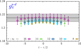
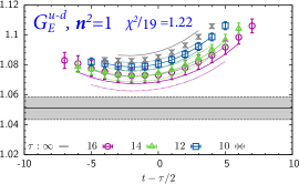
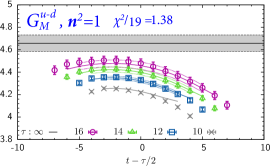
Figure 1: Example of ESC in unrenormalized isovector vector charge $g_{V}^{u-d}$ and form factors $G_{E,M}^{u-d}(\vec{p}^{2})$ at $\vec{p}^{2}=(2\pi/L)^{2}\vec{n}^{2}$ with $\vec{n}^{2}=1$ on $a09m170L$ clover lattices. For $g_{V}^{u-d}$, the $\tau\to\infty$ value (grey band) is the average of the 5 middle data points with $\tau=16$. Fits to $G_{E,M}^{u-d}$ use the $\{4,3^{\ast}\}$ strategy.

Examples of ESC in the vector charge, $g_{V}^{u-d}$, and form factors $G_{E}$ and $G_{M}$ are illustrated in Fig. 1. $g_{V}^{u-d}$ does not vary monotonically with source-sink separation $\tau$, however it is constant to within 1–2%. So we take the average of the central points with the largest $\tau$ (the plateau method). With this choice the identity $Z_{V}g_{V}^{u-d}=1$ is satisfied to within $3\%$ with the $Z_{V}$ calculated in Ref. [5].

Data for the charges, $g_{A,S,T}^{u-d}$, show significant ESC as discussed in [5, 6]. As described in Ref. [1], the key parameter controlling ESC is the energy, $E_{1}$, of the first excited state. Its value, obtained from a 4-state fit to the 2-point function using emperical Bayesian priors [7], is much larger than that of non-interating $N\pi$ or $N\pi\pi$-states, especially for physical $M_{\pi}$ ensembles. Using the energy of the $N\pi$ state as a prior for $E_{1}$ in a 3-state fit gives a much lower output value for $E_{1}$ but with an equally good $\chi^{2}/$DOF, indicating a flat direction in the parameter space. Note that with a small $E_{1}$, even $E_{0}$ is slightly smaller. We have, therefore, analyzed the ESC using multiple strategies and, here, compare two for $g_{A,S,T}^{u-d}$ based on $3^{\ast}$-state fits ($3$-state truncation of the spectral decomposition of the 3-point functions with $\langle 2^{\prime}|\mathcal{O}|2\rangle=0$). The standard $\{4,3^{\ast}\}$ and $\{3^{N\pi},3^{\ast}\}$. In $\{4,3^{\ast}\}$, the spectrum is taken from the standard 4-state fit [8]. In $\{3^{N\pi},3^{\ast}\}$, the energy $E^{N\pi}_{1}$ of the lowest possible state, $N(\mathbf{1})\pi(-\mathbf{1})$, is used as a prior for $E_{1}$ in a 3-state fit and the resulting outputs, ground-state amplitude $A_{0}$ and energies $E_{0}$, $E_{1}$ and $E_{2}$, are used as inputs in fits to the 3-point functions. The data and fits for $\{4,3^{\ast}\}$ and $\{3^{N\pi},3^{\ast}\}$ are compared in Fig. 2 for the $a091m170L$ ensemble, where one expects the largest effect as it has the smallest $M_{\pi}\sim 170$ MeV and $Q_{\rm min}^{2}$, with $Q^{2}=\vec{p}^{2}-(E_{N}-M_{N})^{2}$ being the Euclidean 4-momentum squared transferred.

The value of $g_{A}^{u-d}$ is sensitive to input $E_{1}$ used in the ESC fits, however, different fits are not distinguished by $\chi^{2}/$DOF, again indicating a flat direction. Renormalized charges in the ${\overline{MS}}$ scheme at 2 GeV, $g_{A,S,T}^{u-d}|_{R}=Z_{A,S,T}^{u-d}g_{A,S,T}^{u-d}$, are obtained using $Z_{A,S,T}^{u-d}$ from Ref. [5]. Their chiral-continuum (CC) extrapolation is done using the ansatz $f(a,M_{\pi})=c_{1}+c_{2}a+c_{3}M_{\pi}^{2}$ (see Fig. 3), and the results at $M_{\pi}=135$ MeV and $a=0$ are given in Table 3. The difference in $g_{A}^{u-d}$ is a measure of the systematic uncertainty associated with ESC fits. Data for $g_{S,T}^{u-d}$ from the two strategies, shown in Fig. 3 and the extrapolated values in Table 3, are consistent within $1\sigma$ and the ESC fits do not prefer the low $E^{N\pi}_{1}$.

Ensemble ID	$a$ (fm)	$M_{\pi}$ (MeV)	$L^{3}\times T$	$M_{\pi}L$	$N_{\text{conf}}$	$N^{\text{HP}}_{\text{meas}}$	$N^{\text{LP}}_{\text{meas}}$	$\tau$
$a127m285$	0.127(2)	285(3)	$32^{3}\times 96$	5.85	2002	8008	256,256	{8, 10, 12, 14}
$a094m270$	0.094(1)	270(3)	$32^{3}\times 64$	4.11	2469	7407	237,024	{8, 10, 12, 14, 16}
$a094m270L$	0.094(1)	269(3)	$48^{3}\times 128$	6.16	1854	7416	237,312	{8, 10, 12, 14, 16, 18}
$a091m170$	0.091(1)	170(2)	$48^{3}\times 96$	3.7	2754	11016	352,512	{8, 10, 12, 14, 16}
$a091m170L$	0.091(1)	170(2)	$64^{3}\times 128$	5.08	1825	9125	292,000	{8, 10, 12, 14, 16}
$a073m270$	0.0728(8)	272(3)	$48^{3}\times 128$	4.8	2454	9816	314,112	{11, 13, 15, 17, 19}

Table 1: Lattice parameters of $2+1$-flavor clover ensembles generated by the JLab/W&M/LANL/MIT collaboration. $N^{\text{LP}}_{\text{meas}}$ low-precision and $N^{\text{HP}}_{\text{meas}}$ high-precision measurements of 2- and 3-point functions are made using the bias corrected truncated solver method (see Ref. [5] for details.). $\tau$ gives the source-sink separations studied. Statistics on $a094m270L$, $a091m170$ and $a091m170L$ ensembles are being increased.

Ensemble ID	$a$ (fm)	$M_{\pi}$ (MeV)	$M_{\pi}L$	$L^{3}\times T$	$N_{\text{conf}}^{l}$	$N_{\text{src}}^{l}$	$N_{\text{conf}}^{s}$	$N_{\text{src}}^{s}$	$N_{\text{LP}}/N_{\text{HP}}$
$a15m310$	0.1510(20)	320(5)	3.93	$16^{3}\times 48$	1917	2000	1919	2000	50
$a12m310$	0.1207(11)	310(3)	4.55	$24^{3}\times 64$	1013	5000	1013	1500	30
$a12m220$	0.1184(10)	228(2)	4.38	$32^{3}\times 64$	958	11000	958	4000	30
$a09m310$	0.0888(8)	313(3)	4.51	$32^{3}\times 96$	1081	4000	1081	2000	30
$a09m220$	0.0872(7)	226(2)	4.79	$48^{3}\times 96$	712	8000	847	10000	30/50
$a09m130$	0.0871(6)	138(1)	3.90	$64^{3}\times 96$	1270	10000	877	10000	50
$a06m310$	0.0582(4)	320(2)	3.90	$48^{3}\times 144$	830	4000	956	10000	50
$a06m220$	0.0578(4)	235(2)	4.41	$64^{3}\times 144$	593	10000	554	10000	50
$a06m135$	0.0570(1)	136(1)	3.7	$96^{3}\times 192$	553	500	553	500	50

Table 2: Parameters of the $2+1+1$-flavor HISQ ensembles used for the calculation of disconnected contributions (update of work in Refs. [3, 4]). $N_{\text{conf}}^{l,s}$ gives the number of gauge configurations analyzed for light ($l$) and strange ($s$) flavors. $N_{\text{src}}^{l,s}$ the number of random sources used per configurations, and $N_{\text{LP}}/N_{\text{HP}}$ the ratio of low- to high-precision meausurements. Results for the connected contributions are taken from Ref. [6].

Charge	$\{4,3^{\ast}\}$	$\{3^{N\pi},3^{\ast}\}$
$g_{A}^{u-d}|_{R}$	1.20(5) [0.26]	1.26(5) [0.24]
$g_{S}^{u-d}|_{R}$	1.08(10) [0.32]	1.09(14) [0.49]
$g_{T}^{u-d}|_{R}$	0.95(5) [0.05]	0.94(6) [0.35]

Table 3: $g_{A,S,T}^{u-d}|_{R}$ in $\overline{MS}$ scheme at 2 GeV calculated in 2 ways to remove ESC, and [$\chi^{2}/$DOF] of CC fits.

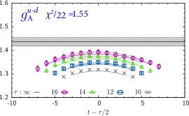
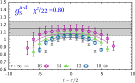
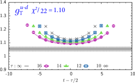
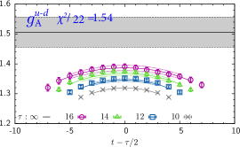
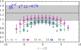
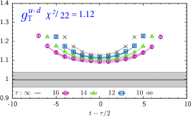
Figure 2: Data and ESC fits for unrenormalized charges $g_{A,S,T}^{u-d}$ on $a09m170L$ clover lattices using the $\{4,3^{\ast}\}$ fit (top 3 panels) and the $\{3^{N\pi},3^{\ast}\}$ fit (bottom 3 panels). Values of $\tau$ and [$\chi^{2}/$DOF] are given in the legend.

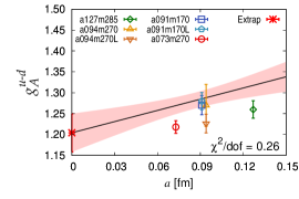
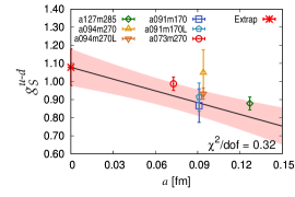
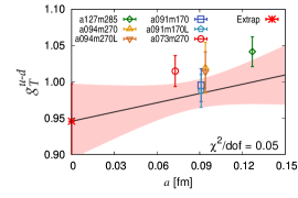
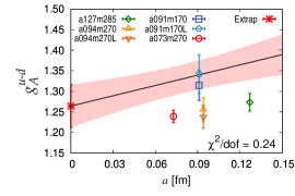
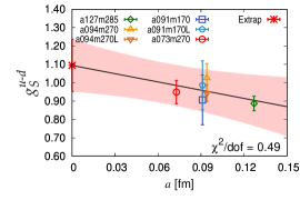
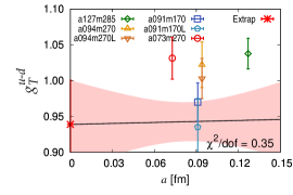
Figure 3: Chiral-continuum extrapolation of the renormalized (in ${\overline{MS}}$ at $2$ GeV) isovector charges using the ansatz $f(a,M_{\pi})=c_{1}+c_{2}a+c_{3}M_{\pi}^{2}$. Results with $\{4,3^{\ast}\}$ ($\{3^{N\pi},3^{\ast}\}$) strategy are shown in the top (bottom) 3 panels. In each pannel, the pink band shows the result of the simultaneous fit plotted versus the lattice spacing $a$ with $M_{\pi}$ set to $135$ MeV. The value in the continuum limit, $a=0$, is marked with a red star.

2 Form factors

We pointed out in Ref. [1] that the large violation of the PCAC relation between axial and pseudoscalar form factors observed in [7] is due to lower energy $N\pi$ excited states that are not exposed by the $\{4,3^{\ast}\}$ analysis. Including them addressed the PCAC relation [1]. We, therefore explore 2 fit strategies here. The top 5 panels in Fig. 4 show renormalized $G_{E}^{u-d}$, $G_{M}^{u-d}$, axial ($G_{A}^{u-d}$), induced pseudoscalar ($\widetilde{G}_{P}^{u-d}$) and pseudoscalar ($G_{P}^{u-d}$) form factors analyzed using the standard $\{4,3^{\ast}\}$ strategy. The bottom 5 panels are with (i) 2-state simultaneous fit to all $V_{\mu}$ channels for $G_{E}$ and $G_{M}$ with $E_{1}$ left free, and (ii) the ${S}_{A4}$ strategy defined in [1] for the axial channels.

The $G_{E}$ and $G_{M}$ data show better collapse onto a single curve (indicating no significant $a$, $M_{\pi}$, volume dependence) plotted versus $Q^{2}/M_{N}^{2}$, and the agreement with the Kelly curve is better compared to the clover-on-HISQ data discussed in Ref. [8]. The main difference between the two strategies is in the errors: the errors from the simultaneous fits are larger, especially at the larger $Q^{2}$.

In the axial channels, data with ${S}_{A4}$ satisfies PCAC with most of the change occuring in $\widetilde{G}_{P}^{u-d}$ and $G_{P}^{u-d}$ as discussed in [1]. Note that data for $G_{A}^{u-d}$, $\widetilde{G}_{P}^{u-d}$ and $G_{P}^{u-d}$, shown in Fig. 4, will move up or down depending on the value of $g_{A}$, which, as shown in Tab. 3, has unresolved systematics. Thus, resolving the ESC in $g_{A}$ is essential before comparing/using $G_{A}(Q^{2})$ in phenomenology.

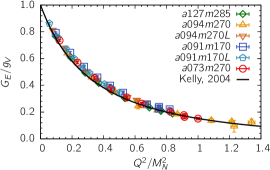
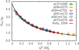
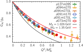
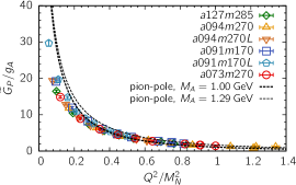
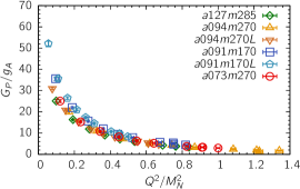
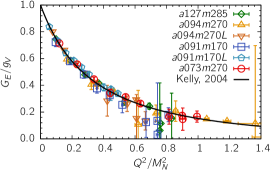
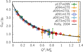
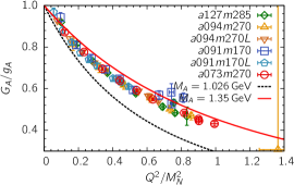
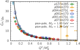
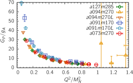
Figure 4: Renormalized isovector form factors ($G_{E}^{u-d}$, $G_{M}^{u-d}$, $G_{A}^{u-d}$, $\widetilde{G}_{P}^{u-d}$ and $G_{P}^{u-d}$) versus $Q^{2}/M_{N}^{2}$. Top (bottom) 5 panels show data with standard $\{4,3^{\ast}\}$ (new) strategy. The value of $g_{A}$ is taken from $\{4,3^{\ast}\}$ fit.

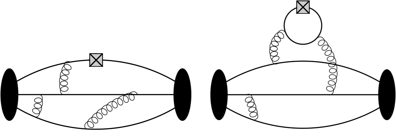
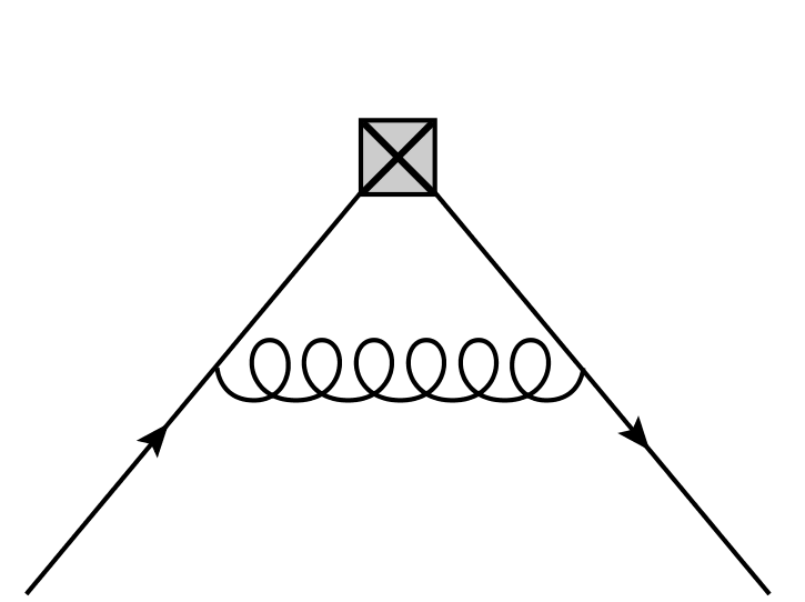
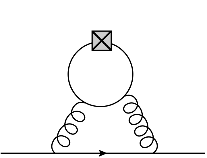
Figure 5: Connected and disconnected diagrams for (i) the 3-point functions that give nucleon charges (left 2 panels) and (ii) the renormalization of the flavor diagonal quark bilinear operators in 3-flavor theory (right 2).

3 Flavor diagonal charges on $2+1+1$-flavor HISQ lattices

The flavor diagonal charges presented here are obtained using the same ESC strategy as discussed in [3, 4]. Alternate analyses taking into account possible lower excited states are in progress. The connected and disconnected contributions shown in Fig. 5 are analyzed separately to construct the renormalized charges $g_{A,S,T}^{f}|_{R}=Z^{ff^{\prime}}_{A,S,T}(g_{A,S,T}^{f^{\prime},\text{conn}}+g_{A,S,T}^{f^{\prime},\text{disc}})$, where $f,f^{\prime}$ are quark flavors. The connected contribution, $g_{A,S,T}^{f,\text{conn}}$, are taken from Ref. [6]. Here, we update $g_{\Gamma}^{f,\text{disc}}$ using the larger data set shown in Table 2, and present new results on the connected and disconnected contributions (right two panels in Fig. 5) for the renormalization matrix $Z^{ff^{\prime}}_{A,S,T}$ in the 3-flavor theory using the RI-sMOM scheme. The matching between the lattice RI-sMOM and continuum ${\overline{MS}}$ schemes, and the running to 2 GeV are done using 2-loop perturbation theory. Additionally, we give our first preliminary data for the scalar charges.

The new data for $Z$ factors in Table 4 show that the difference between the isovector ($u-d$) and isoscalar ($u+d$) renormalization constants for the axial and tensor operators is small for all 4 values of $a$. This validates the approximation $g_{A,T}^{u+d}|_{R}={Z_{A,T}^{u+d,u+d}}g_{A,T}^{u+d}+Z_{A,T}^{u+d,s}g_{A,T}^{s}\approx Z_{A,T}^{u-d}g_{A,T}^{u+d}$ made in Refs. [3, 4] for our clover-on-HISQ calculations. Also, the off-diagonal mixing $Z_{A,T}^{u+d,s}g_{A,T}^{s}$ is tiny since $Z_{A,T}^{u+d,s}\lesssim 0.1$ and the purely disconnected contributions are even smaller: $g_{A}^{s}\approx 0.05$ and $g_{T}^{s}\approx 0.002$. With only 8 data points, the chiral-continuum extrapolations of the disconnected contributions $g_{A,T}^{l,s,\text{disc}}|_{R}$ are carried out using the simple ansatz $g(a,M_{\pi})=c_{1}+c_{2}a+c_{3}M_{\pi}^{2}$ and the data and fits are shown in Fig 6. Combining the disconnected contributions with the connected contributions $g_{A,T}^{l,\text{conn}}|_{R}$ presented in Ref. [6], our preliminary updated flavor diagonal charges are

$$g_{A}^{u}|_{R} =0.790(23)(30) g_{A}^{d}|_{R} =-0.425(15)(30) g_{A}^{s}|_{R} =-0.053(7)$$ (1)

$$g_{T}^{u}|_{R} =0.783(27)(10) g_{T}^{d}|_{R} =-0.205(10)(10) g_{T}^{s}|_{R} =-0.0022(12)\,,$$ (2)

where the second is a systematic error assigned to the chiral-continuum extrapolation [6].

a	$Z_{A}^{u-d}/{Z_{V}^{u-d}}$	${Z_{A}^{u+d,u+d}}/{Z_{V}^{u-d}}$
0.15	1.080(13)	1.0856(11)
0.12	1.061(11)	1.073(11)
0.09	1.0380(40)	1.0484(32)
0.06	1.0227(19)	1.0383(28)

a	$Z_{T}^{u-d}/{Z_{V}^{u-d}}$	${Z_{T}^{u+d,u+d}}/{Z_{V}^{u-d}}$
0.15	1.032(18)	1.031(19)
0.12	1.0538(76)	1.0541(68)
0.09	1.0795(34)	1.0796(34)
0.06	1.0956(70)	1.0959(70)

Table 4: Renormalization factors $Z_{A}$ and $Z_{T}$ for $u-d$ (isovector) and $u+d$ (isoscalar) operators in ${\overline{MS}}$ scheme at $2$ GeV on HISQ lattices. Renormalizing using ratios with $Z_{V}^{u-d}$ is intended to cancel some of the statistical and systematic uncertainties as discussed in Ref. [6]. Errors quoted are the larger of the two: half the difference between RI-MOM and RI-sMOM results or the largest statistical error.

There remain issues regarding the systematics in the calculation of the matrix element of the scalar operator that are still being investigated: the values for the the renormalization constants, $Z_{S}$, show significant differences between the RI-MOM and RI-sMOM schemes. For example, there are $5\sim 30\%$ differences in $Z_{S}^{u-d}$, and $5\sim 10\%$ differences in $Z_{S}^{u+d,u+d}$ with the differences increasing as the lattice spacing becomes larger. For the mixing matrix element $Z_{S}^{s,u+d}$, the RI-MOM scheme gives $-0.04\sim-0.1$, which is much larger than the RI-sMOM scheme result of $-0.003\sim-0.02$. In fact, in the calculation of strangeness, $g_{S}^{s}|_{R}={Z_{S}^{s,s}}g_{S}^{s}+Z_{S}^{s,u+d}g_{S}^{u+d}$, the larger value of mixing $Z_{S}^{s,u+d}$ in RI-MOM scheme gives a negative value for $g_{S}^{s}|_{R}$! For the time being, we use the RI-sMOM scheme, in which case the corresponding mixing term $Z_{S}^{s,u+d}g_{S}^{u+d}$ gives about $6\sim 20\%$ correction to the diagonal term ${Z_{S}^{s,s}}g_{S}^{s}$.

The renormalized strangeness $g_{S}^{s}|_{R}$, from the clover-on-HISQ calculation, is plotted versus $a$ and $M_{\pi}^{2}$ in Fig. 7, along with the nucleon sigma term $\sigma_{\pi N}=m_{l}g_{S}^{u+d}$ that is independent of the renormalization scheme. We have used $am_{l}=\frac{1}{2}(\kappa^{-1}-\kappa_{\text{crit}}^{-1})$ for the definition of the bare quark mass and $g_{S}^{u+d}=g_{S}^{u+d,\text{conn}}+g_{S}^{u+d,\text{disc}}$ for the unrenormalized isoscalar scalar charge. The data show a significant $a$ dependence in $g_{S}^{s}|_{R}$ while the large linear dependence of $\sigma_{\pi N}$ on $M_{\pi}^{2}$ comes from the quark mass in the definition of $\sigma_{\pi N}$. The dependence of $g_{S}^{u+d}|_{R}$ on $a$ and of $g_{S}^{s}|_{R}$ on $M_{\pi}^{2}$ is not clear.

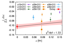
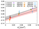
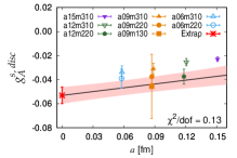
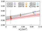
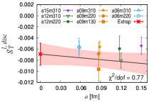
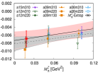
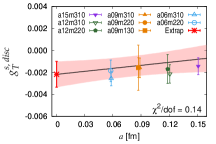
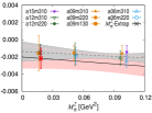
Figure 6: The extrapolation of the disconnected contributions of the renormalized (in ${\overline{MS}}$ at $2$ GeV) flavor diagonal charges $g_{A}^{l(s),\text{disc}}|_{R}$ (top row) and $g_{T}^{l(s),\text{disc}}|_{R}$ (bottom row) using the chiral-continuum fit ansatz $g(a,M_{\pi})=c_{1}+c_{2}a+c_{3}M_{\pi}^{2}$. The parameters for the eight clover-on-HISQ ensembles are given in Table 2.

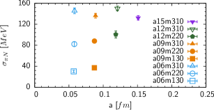
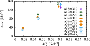
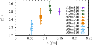
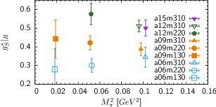
Figure 7: (Top) The nucleon sigma term $\sigma_{N\pi}$ plotted versus $a$ and $M_{\pi}^{2}$. (Bottom) The nucleon strangeness $g_{s}^{s}|_{R}$ renormalized in ${\overline{MS}}$ scheme at $2$ GeV versus $a$ and $M_{\pi}^{2}$.

Conclusions: We have presented the status of ongoing calculations of nucleon matrix elements and are performing a more detailed analysis of the excited state contamination in the extraction of all nucleon matrix elements. The analysis of flavor diagonal scalar charges, $g^{u,d,s}_{S}$ is new, however, a complete understanding of all the systematics is still under investigation.

Acknowledgments: We thank the MILC collaboration for sharing their $2+1+1$-flavor HISQ ensembles. Simulations were carried out on computer facilities at (i) the National Energy Research Scientific Computing Center, a DOE Office of Science User Facility supported under Contract No. DE-AC02-05CH11231; and, (ii) the Oak Ridge Leadership Computing Facility supported by the Office of Science of the DOE under Contract No. DE-AC05-00OR22725; (iii) the USQCD Collaboration, which are funded by the Office of Science of the U.S. Department of Energy, and (iv) Institutional Computing at Los Alamos National Laboratory. T. Bhattacharya and R. Gupta were partly supported by the U.S. Department of Energy, Office of Science, Office of High Energy Physics under Contract No. DE-AC52-06NA25396. S. Park, T. Bhattacharya, R. Gupta, Y.-C. Jang and B. Yoon were partly supported by the LANL LDRD program.

References

- [1] Y.-C. Jang, R. Gupta, B. Yoon, and T. Bhattacharya 1905.06470.
- [2] MILC Collaboration, A. Bazavov et al. Phys. Rev. D87 (2013), no. 5 054505, [1212.4768].
- [3] H.-W. Lin, R. Gupta, B. Yoon, Y.-C. Jang, and T. Bhattacharya Phys. Rev. D98 (2018), no. 9 094512, [1806.10604].
- [4] R. Gupta, B. Yoon, T. Bhattacharya, V. Cirigliano, Y.-C. Jang, and H.-W. Lin Phys. Rev. D98 (2018), no. 9 091501, [1808.07597].
- [5] B. Yoon et al. Phys. Rev. D95 (2017), no. 7 074508, [1611.07452].
- [6] R. Gupta, Y.-C. Jang, B. Yoon, H.-W. Lin, V. Cirigliano, and T. Bhattacharya Phys. Rev. D98 (2018) 034503, [1806.09006].
- [7] R. Gupta, Y.-C. Jang, H.-W. Lin, B. Yoon, and T. Bhattacharya Phys. Rev. D96 (2017), no. 11 114503, [1705.06834].
- [8] Y.-C. Jang, R. Gupta, H.-W. Lin, B. Yoon, and T. Bhattacharya Phys. Rev. D101 (2020) 014507, [1906.07217].