A curve shortening equation with time-dependent mobility related to grain boundary motions

Abstract.

A curve shortening equation related to the evolution of grain boundaries is presented. This equation is derived from the grain boundary energy by applying the maximum dissipation principle. Gradient estimates and large time asymptotic behavior of solutions are considered. In the proof of these results, one key ingredient is a new weighted monotonicity formula that incorporates a time-dependent mobility.

1. Introduction

We study a curve shortening equation related to the evolution of grain boundaries. Most materials have a polycrystalline microstructure composed of a myriad of tiny single crystalline grains separated by grain boundaries. Many experimental results indicate that the microscale structure of the grain boundaries is strongly related to the macroscale properties of the material composed of these grain boundaries.

Mathematical modeling of the grain boundaries was first studied by Mullins and Herring [9, 15, 16]. In particular when the grain boundary energy depends only on the length and shape of these grain boundaries, a curve shortening equation or a mean curvature flow equation is obtained. Both equations are quasilinear and underlie important problems in geometric analysis; hence there is a diversity of research looking into these problems.

However, from the perspective of research on grain boundaries, it is also important to treat other state variables. For instance, grain boundaries are regarded as some singularity in lattice orientation of each grain. Kinderlehrer-Liu [11] introduced misorientations, which are the differences in lattice orientation of two grains separated by a grain boundary, as a parameter in the expression for the grain boundary energy. They derived geometric evolution equations based on the maximal dissipation principle. Epshteyn-Liu-Mizuno [7, 6] considered the case that the misorientation depends on the time and demonstrated the local existence of network solutions provided the grain boundaries are straight line segments. Nevertheless, the interaction between curvature and misorientation is not well-known.

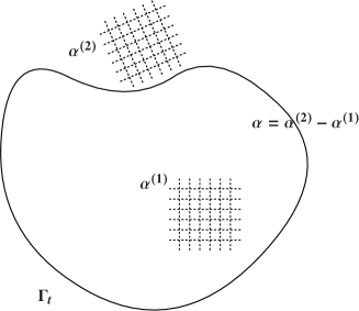
Figure 1. Let $\Gamma_{t}\subset\mathbb{R}^{2}$ be a smooth Jordan curve, and let $\alpha^{(1)}$, $\alpha^{(2)}$ be time-dependent unknown functions, called orientations. The difference $\alpha=\alpha^{(2)}-\alpha^{(1)}$ is called the misorientation.

In this article, we study the grain boundary energy that include time-dependent misorientations as a state variable. First, we consider a smooth Jordan curve $\Gamma_{t}\subset\mathbb{R}^{2}$ as a grain boundary, with $v_{n}$ and $\kappa$ denoting the normal velocity and the curvature of $\Gamma_{t}$, respectively. We assume that the misorientation $\alpha(t)=\alpha^{(2)}(t)-\alpha^{(1)}(t)$ depends on the time and is independent of the position vector of the grain boundary(See Figure 1). Taking the grain boundary energy as

$$\int_{\Gamma_{t}}\sigma(\alpha)\,d\mathscr{H}^{1}=\sigma(\alpha)|\Gamma_{t}|,$$

we derived a system of evolution equations obtained from the maximum dissipation principle:

(1.1) $$\left\{\begin{aligned} v_{n}&=\mu\sigma(\alpha)\kappa,&\quad&\text{on}\ \Gamma_{t},\ t>0,\\ \alpha_{t}&=-\gamma\sigma_{\alpha}(\alpha)|\Gamma_{t}|,&\quad&t>0.\end{aligned}\right.$$

Here, $\mu$ and $\gamma$ denote positive constants, $\sigma:\mathbb{R}\to[0,\infty)$ denotes a given smooth function, and $|\Gamma_{t}|$ the length of $\Gamma_{t}$. We present a derivation of (1.1) in Section 2. Our system consists of two equations, one being a curve shortening equation with time-dependent mobility, and the other describing the evolution of the misorientation. The most significant difference between the PDE in [11] and (1.1) is the time-dependent misorientation. The evolution of a misorientation was considered in [7, 6]. However, only the relaxation limit $\mu\rightarrow\infty$ was studied, namely, the authors employed straight line segments to be grain boundaries. On the other hand, they considered curved grain boundaries in the derivation of the system. For this reason, understanding the relationship between the effect of curvature and the evolution of misorientations is important.

In regard to curve shortening flow, specifically time-independent misorientations, a solution of (1.1) exists in a finite time if the initial data is a Jordan curve. For example, if $\inf_{\alpha\in\mathbb{R}}\sigma(\alpha)>C$ and $\tilde{\Gamma}_{0}=\{|x|=R\}$ for some constants $C>0$ and $R>0$, then the solution $(\tilde{\Gamma}_{t},\tilde{\alpha})$ of (1.1) with the initial data $(\tilde{\Gamma}_{0},\tilde{\alpha}_{0})$ is also a circle and the radius $r(t)$ coincides with

$$\sqrt{R^{2}-2\mu\int_{0}^{t}\sigma(\tilde{\alpha}(s))ds}.$$

Note that the comparison principle implies $\Gamma_{t}\subset\{|x|\leq\sqrt{R^{2}-2\mu Ct}\}$ for any solution $(\Gamma_{t},\alpha)$ such that $\Gamma_{0}\subset\{|x|\leq R\}$, since $\{|x|=\sqrt{R^{2}-2\mu Ct}\}$ is a solution of $v_{n}=\mu C\kappa$. Therefore, any solution starting from a Jordan curve disappears in a finite time. In contrast, as for curve shortening flow, the solution is expected to converge to a straight line under suitable conditions, although the effects from boundary conditions and junctions also need to be considered (see Example 2.4). The mean curvature flow of the graph has been studied in [3, 4, 5], but is not well-known in regard to effects concerning the evolving misorientations. Consequently, to understand the nature of the time global classical solution of (1.1), we consider two unbounded grains, and their grain boundary represented by a periodic graph (see (2.18) below). In this situation, we study the properties of the time global solutions.

To obtain the solvability of the system in the graphical setting, a priori gradient estimates for solutions of our system play an important role. For the curve shortening equation with constant mobility, Huisken [10] derived the so-called monotonicity formula (cf. [8]) and Ecker-Huisken[4] provided gradient estimates for the entire graph using Huisken’s monotonicity formula (See also [14, 18]. Sharp gradient estimates are given in [1]). Key ingredients of Huisken’s monotonicity formula are the properties of the standard backward heat kernel. We derive the weighted monotonicity formula in similar manner as for Huisken’s formula(cf. Ecker [2, Theorem 4.13]) for the curve shortening equation with a time-dependent mobility (see Theorem 3.1 below). Then, using the weighted monotonicity formula we obtain gradient estimates and the global existence of solutions for the problem (see Theorem 4.2 and Theorem 4.5 below). Our new argument is to replace the standard backward heat kernel with one with time-dependent thermal conductivity. Finally, we prove that the time global solution converges to a straight line exponentially in $C^{2}$ (see Theorem 5.1).

The paper is organized as follows. In Section 2, we set up the model and derive evolution equations using the maximum dissipation principle. We consider a graph of an unknown function as a grain boundary and derive a governing equation from the model. In Section 3, we briefly review backward heat kernels with time-dependent thermal conductivity. Next, we obtain the weighted monotonicity identity for our problem. Using this identity, we derive gradient estimates and the global existence of solutions to our problem in Section 4. In Section 5, we deduce the large time asymptotic behavior of the global solution.

2. Derivation of the system

We begin by deriving the governing equations of our systems from the energy dissipation principle. This approach is taken from [7, 6], without the effect of the triple junction drag. We consider a single grain boundary $\Gamma_{t}$ represented by point vector $\bm{\xi}(s,t)\in\mathbb{R}^{2}$ for $0\leq s\leq 1$ and $t>0$. Note that $s$ is not necessarily the arclength parameter. To understand the relationship between misorientations and the effect of curvature, we impose the periodic boundary condition, specifically $\bm{\xi}(0,t)=\bm{\xi}(1,t)$ and $\bm{\xi}_{s}(0,t)=\bm{\xi}_{s}(1,t)$ for $t>0$. We denote a tangent vector by $\bm{b}=\bm{\xi}_{s}$ and a normal vector by $\bm{n}=R\bm{b}$ where $R$ is a matrix describing an anti-clockwise rotation through angle $\pi/2$. Again we remark that the tangent vector $\bm{b}$ and the normal vector $\bm{n}$ are not necessarily unit vectors because in general $s$ is not the arclength parameter.

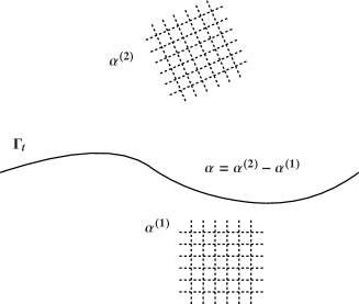
Figure 2. Model of a single grain boundary $\Gamma_{t}$. State variables $\alpha^{(1)}$ and $\alpha^{(2)}$ represent the lattice orientations of the grains. State variable $\alpha=\alpha^{(2)}-\alpha^{(1)}$ defines the misorientation on the grain boundary $\Gamma_{t}$.

Next, we let $\alpha=\alpha(t)$ be the lattice misorientation on the grain boundary $\Gamma_{t}$. We assume that the lattice misorientation $\alpha$ depends on time $t$, but is independent of parameter $s$. We consider the normal vector $\bm{n}$ and the lattice misorientation $\alpha$ as state variables so we define the interfacial grain boundary energy density of $\Gamma_{t}$ as

$$\sigma=\sigma(\bm{n},\alpha)\geq 0.$$

Thus the total grain boundary energy of the system $\Gamma_{t}$ is written

(2.1) $$E(t)=\int_{\Gamma_{t}}\sigma(\bm{n},\alpha)\,d\mathscr{H}^{1}=\int_{0}^{1}\sigma(\bm{n}(s,t),\alpha(t))|\bm{b}(s,t)|\,ds,$$

where $\mathscr{H}^{1}$ is the $1$-dimensional Hausdorff measure and $|\cdot|$ is the standard Euclidean vector norm on $\mathbb{R}^{2}$. Next, we assume that $\sigma$ is a non-negative smooth function and positively homogeneous of degree $0$ in $\bm{n}$.

Let us now derive the grain boundary motion from the dissipation principle of the total grain boundary energy (2.1). Let $\hat{\ }$ be the normalization operator of vectors, e.g., $\hat{\bm{b}}=\frac{\bm{b}}{|\bm{b}|}$. Next, we compute the dissipation rate of the total grain boundary energy $E(t)$ at time $t$,

(2.2) $$\begin{split}\frac{d}{dt}E(t)&=\int_{0}^{1}\sigma_{\bm{n}}\cdot\frac{d\bm{n}}{dt}|\bm{b}|\,ds+\int_{0}^{1}\sigma\frac{\bm{b}}{|\bm{b}|}\cdot\frac{d\bm{b}}{dt}\,ds+\int_{0}^{1}\sigma_{\alpha}\frac{d\alpha}{dt}|\bm{b}|\,ds\\ &=\int_{0}^{1}\left(|\bm{b}|\mathstrut^{t}\!R\sigma_{\bm{n}}+\sigma\hat{\bm{b}}\right)\cdot\frac{d\bm{b}}{dt}\,ds+\int_{0}^{1}\sigma_{\alpha}\frac{d\alpha}{dt}|\bm{b}|\,ds.\end{split}$$

Now, consider a polar angle $\theta$ for $\bm{n}$ and set $\bm{n}=|\bm{n}|(\cos\theta,\sin\theta)$. Since $\sigma$ is positively homogeneous of degree $0$ in $\bm{n}$, we have

(2.3) $$0 =\frac{d}{d\lambda}\sigma(\lambda\bm{n},\alpha)\bigg{|}_{\lambda=1}=\sigma_{\bm{n}}(\bm{n},\alpha)\cdot\bm{n}, \quad\mathstrut{}^{t}\!R\sigma_{\bm{n}} =(\mathstrut{}^{t}\!R\sigma_{\bm{n}}\cdot\hat{\bm{n}})\hat{\bm{n}},$$

$$\sigma_{\theta} :=\frac{d}{d\theta}\sigma(\bm{n},\alpha)=|\bm{n}|\mathstrut{}^{t}\!R\sigma_{\bm{n}}\cdot\hat{\bm{n}}, \quad\sigma_{\theta}\hat{\bm{n}} =|\bm{b}|\mathstrut^{t}\!R\sigma_{\bm{n}},$$

and thus, we define the vector $\bm{T}$ known as the line tension vector,

$$\bm{T}:=\sigma_{\theta}\hat{\bm{n}}+\sigma\hat{\bm{b}}=|\bm{b}|\mathstrut^{t}\!R\sigma_{\bm{n}}+\sigma\hat{\bm{b}}.$$

Next, using a change of variable

(2.4) $$\frac{d\bm{b}}{dt}=\frac{d}{ds}\frac{d\bm{\xi}}{dt},$$

we rewrite (2.2) as

(2.5) $$\frac{d}{dt}E(t)=\int_{0}^{1}\bm{T}\cdot\frac{d}{ds}\frac{d\bm{\xi}}{dt}\,ds+\int_{0}^{1}\sigma_{\alpha}\frac{d\alpha}{dt}|\bm{b}|\,ds=-\int_{0}^{1}\bm{T}_{s}\cdot\frac{d\bm{\xi}}{dt}\,ds+\int_{0}^{1}\sigma_{\alpha}\frac{d\alpha}{dt}|\bm{b}|\,ds$$

from the periodic condition $\bm{b}(0,t)=\bm{b}(1,t)$.

For the reader’s convenience, we recall a property of the derivative of the line tension vector $\bm{T}$.

Lemma 2.1 (cf. [11]).

Let $\kappa$ be the curvature of $\Gamma_{t}$. Then

(2.6) $$\bm{T}_{s}=|\bm{b}|(\sigma_{\theta\theta}+\sigma)\kappa\hat{\bm{n}}.$$

Proof.

Denote $\partial_{\Gamma_{t}}=\frac{1}{|\bm{b}|}\partial_{s}$, which is the arc-length derivative along with $\Gamma_{t}$. From the Frenet-Serret formula, we obtain

(2.7) $$\hat{\bm{b}}_{s}=|\bm{b}|\partial_{\Gamma_{t}}\hat{\bm{b}}=|\bm{b}|\kappa\hat{\bm{n}},\quad\hat{\bm{n}}_{s}=|\bm{b}|\partial_{\Gamma_{t}}\hat{\bm{n}}=-|\bm{b}|\kappa\hat{\bm{b}}.$$

Hence, we obtain,

(2.8) $$\begin{split}\bm{T}_{s}&=\left(\sigma_{\bm{n}\theta}\cdot\bm{n}_{s}\right)\hat{\bm{n}}+\sigma_{\theta}\hat{\bm{n}}_{s}+\left(\sigma_{\bm{n}}\cdot\bm{n}_{s}\right)\hat{\bm{b}}+\sigma\hat{\bm{b}}_{s}\\ &=\left(\mathstrut{}^{t}\!R\sigma_{\bm{n}\theta}\cdot\bm{b}_{s}+|\bm{b}|\sigma\kappa\right)\hat{\bm{n}}+\left(-|\bm{b}|\sigma_{\theta}\kappa+\mathstrut^{t}\!R\sigma_{\bm{n}}\cdot\bm{b}_{s}\right)\hat{\bm{b}}.\end{split}$$

Since $\sigma$ and $\sigma_{\theta}$ are positively homogeneous of degree $0$ in $\bm{n}$, as the similar calculation on (2.3), we have

(2.9) $$\sigma_{\theta}\hat{\bm{n}}=|\bm{b}|\mathstrut^{t}\!R\sigma_{\bm{n}},\quad\sigma_{\theta\theta}\hat{\bm{n}}=|\bm{b}|\mathstrut^{t}\!R\sigma_{\bm{n}\theta}.$$

Using the orthogonal relation $\bm{b}\cdot\hat{\bm{n}}=0$ and the Frenet-Serret formula (2.7), we obtain $\bm{b}_{s}\cdot\hat{\bm{n}}=-\bm{b}\cdot\hat{\bm{n}}_{s}=|\bm{b}|^{2}\kappa$. Thus, from (2.9)

$$\begin{split}\mathstrut{}^{t}\!R\sigma_{\bm{n}\theta}\cdot\bm{b}_{s}+|\bm{b}|\sigma\kappa&=\frac{1}{|\bm{b}|}\sigma_{\theta\theta}\hat{\bm{n}}\cdot\bm{b}_{s}+|\bm{b}|\sigma\kappa=|\bm{b}|\left(\sigma_{\theta\theta}+\sigma\right)\kappa,\\ -|\bm{b}|\sigma_{\theta}\kappa+\mathstrut^{t}\!R\sigma_{\bm{n}}\cdot\bm{b}_{s}&=-|\bm{b}|\sigma_{\theta}\kappa+\frac{1}{|\bm{b}|}\sigma_{\theta}\hat{\bm{n}}\cdot\bm{b}_{s}=0\end{split}$$

and hence we derive (2.6). ∎

To ensure that the whole system is dissipative, i.e.

$$\frac{d}{dt}E(t)\leq 0,$$

we impose the so called Mullins equation or the curve shortening equation for the evolution of the grain boundary $\Gamma_{t}$. From Lemma 2.1, $\bm{T}_{s}$ is proportional to the normal vector on $\Gamma_{t}$ and therefore we impose

(2.10) $$v_{n}=\mu\partial_{\Gamma_{t}}\bm{T}\cdot\hat{\bm{n}}=\mu(\sigma_{\theta\theta}+\sigma)\kappa\quad\text{on}\ \Gamma_{t},$$

where $v_{n}$ denotes the normal velocity vector of $\Gamma_{t}$ and $\mu>0$ a positive mobility constant. Note that equation (2.10) may be derived from the variation of the energy $E$ with respect to the curve $\bm{\xi}$. Indeed, for any test function $\bm{\phi}\in C^{\infty}_{0}(0,1)$,

(2.11) $$\begin{split}\frac{\delta E}{\delta\bm{\xi}}[\bm{\phi}]&=\int_{0}^{1}\left((\sigma_{\bm{n}}(\bm{n},\alpha)\cdot R\bm{\phi}_{s})|\bm{b}|+\sigma(\bm{n},\alpha)\hat{\bm{b}}\cdot\bm{\phi}_{s}\right)\,ds\\ &=\int_{0}^{1}\left(|\bm{b}|\mathstrut^{t}\!R\sigma_{\bm{n}}(\bm{n},\alpha)+\sigma(\bm{n},\alpha)\hat{\bm{b}}\right)\cdot\bm{\phi}_{s}\,ds\\ &=-\int_{\Gamma_{t}}\partial_{\Gamma_{t}}\left(|\bm{b}|\mathstrut^{t}\!R\sigma_{\bm{n}}(\bm{n},\alpha)+\sigma(\bm{n},\alpha)\hat{\bm{b}}\right)\cdot\bm{\phi}\,d\mathscr{H}^{1},\end{split}$$

thus (2.10) is turned into

$$\frac{d\bm{\xi}}{dt}=-\mu\frac{\delta E}{\delta\bm{\xi}}.$$

Since $v_{n}=\bm{\xi}_{t}\cdot\hat{\bm{n}}$, we obtain

(2.12) $$\bm{T}_{s}\cdot\frac{d\bm{\xi}}{dt}=\frac{1}{\mu}|v_{n}|^{2}|\bm{b}|\geq 0.$$

Next, we consider the law underlying evolution of lattice misorientations. Since $\alpha$ is independent of the parameter $s$,

$$\int_{0}^{1}\sigma_{\alpha}\frac{d\alpha}{dt}|\bm{b}|\,ds=\frac{d\alpha}{dt}\int_{0}^{1}\sigma_{\alpha}|\bm{b}|\,ds=\frac{d\alpha}{dt}\int_{\Gamma_{t}}\sigma_{\alpha}\,d\mathscr{H}^{1},$$

hence for a constant $\gamma>0$, we impose the following relation for the rate of change of the lattice misorientation;

(2.13) $$\frac{d\alpha}{dt}=-\gamma\int_{\Gamma_{t}}\sigma_{\alpha}\,d\mathscr{H}^{1},$$

to ensure the whole system is dissipative, namely $\frac{d}{dt}E(t)\leq 0$. Note that our proposed equation (2.13) can be derived from the variation of the energy $E$ with respect to lattice misorientation $\alpha$. Indeed for any number $\xi\in\mathbb{R}$,

$$\frac{\delta E}{\delta\alpha}[\xi]=\frac{d}{d\varepsilon}\bigg{|}_{\varepsilon=0}\int_{0}^{1}\sigma(\bm{n},\alpha+\varepsilon\xi)|\bm{b}|\,ds=\xi\int_{0}^{1}\sigma_{\alpha}(\bm{n},\alpha)|\bm{b}|\,ds,$$

thus (2.13) becomes

(2.14) $$\frac{d\alpha}{dt}=-\gamma\frac{\delta E}{\delta\alpha}.$$

Now, substituting equations (2.10) and (2.13) in the rate of change for the total energy (2.5), we find that the whole system is dissipative, namely

(2.15) $$\frac{d}{dt}E(t)=-\frac{1}{\mu}\int_{\Gamma_{t}}|v_{n}|^{2}\,d\mathscr{H}^{1}-\frac{1}{\gamma}\left|\frac{d\alpha}{dt}\right|^{2}\leq 0.$$

Remark 2.2.

We emphasize in (2.15) that the evolving misorientation $\alpha$ has a dissipative structure. See also [7]. In contrast, the misorientation is a fixed parameter in [11].

We next consider the grain boundary motion for the isotropic case. The grain boundary energy density $\sigma$ is independent of the normal vector $\bm{n}$. Then, the equations (2.10) and (2.13) become

(2.16) $$\left\{\begin{aligned} v_{n}&=\mu\sigma(\alpha)\kappa,&\quad&\text{on}\ \Gamma_{t},\ t>0,\\ \alpha_{t}&=-\gamma\sigma_{\alpha}(\alpha)|\Gamma_{t}|,&\quad&t>0.\end{aligned}\right.$$

Imposing the periodic boundary condition, we put $\mathbb{T}:=\mathbb{R}/\mathbb{Z}$ and write $\Gamma_{t}$ as a graph of an unknown function $u=u(x,t)$ on $\mathbb{T}\times[0,\infty)$, namely

(2.17) $$\bm{\xi}(x,t)=(x,u(x,t)),\quad x\in\mathbb{T},\quad t>0.$$

With the initial data $\bm{\xi}(x,0)=(x,u_{0}(x))$, $\alpha(0)=\alpha_{0}\in\mathbb{R}$, and the periodic boundary condition $\bm{\xi}(0,t)=\bm{\xi}(1,t)$, $\bm{\xi}_{s}(0,t)=\bm{\xi}_{s}(1,t)$, equation (2.16) becomes

(2.18) $$\left\{\begin{aligned} \frac{u_{t}}{\sqrt{1+|u_{x}|^{2}}}&=\mu\sigma(\alpha)\left(\frac{u_{x}}{\sqrt{1+|u_{x}|^{2}}}\right)_{x},&\quad&x\in\mathbb{T},\ t>0,\\ \alpha_{t}&=-\gamma\sigma_{\alpha}(\alpha)|\Gamma_{t}|,&\quad&t>0,\\ u(0,t)&=u(1,t),\quad u_{x}(0,t)=u_{x}(1,t),&\quad&t>0,\\ u(x,0)&=u_{0}(x),&\quad&x\in\mathbb{T},\\ \alpha(0)&=\alpha_{0}.\end{aligned}\right.$$

Indeed, the normal velocity $v_{n}$ and the curvature $\kappa$ are given by

$$\begin{split}v_{n}&=\bm{\xi}_{t}\cdot\hat{\bm{n}}=(0,u_{t})\cdot\left(\frac{1}{\sqrt{1+|u_{x}|^{2}}}(-u_{x},1)\right)=\frac{u_{t}}{\sqrt{1+|u_{x}|^{2}}},\\ \kappa&=\partial_{\Gamma_{t}}\hat{\bm{b}}\cdot\hat{\bm{n}}=\frac{1}{\sqrt{1+|u_{x}|^{2}}}\left(\frac{1}{\sqrt{1+|u_{x}|^{2}}}(1,u_{x})\right)_{x}\cdot\left(\frac{1}{\sqrt{1+|u_{x}|^{2}}}(-u_{x},1)\right)\\ &=\left(\frac{u_{x}}{\sqrt{1+|u_{x}|^{2}}}\right)_{x}.\end{split}$$

From (2.1), the associated total grain boundary energy $E(t)$ is given by

(2.19) $$E(t)=\int_{\Gamma_{t}}\sigma(\alpha)=\sigma(\alpha)\int_{0}^{1}\sqrt{1+|u_{x}|^{2}}\,dx.$$

Proposition 2.3 (Free energy dissipation).

Let $u$ be a solution of (2.18). Then

(2.20) $$\frac{dE}{dt}=-\frac{1}{\gamma}|\alpha_{t}|^{2}-\frac{1}{\mu}\int_{0}^{1}\left(\frac{u_{t}}{\sqrt{1+|u_{x}|^{2}}}\right)^{2}\sqrt{1+|u_{x}|^{2}}\,dx.$$

Proof.

By direct calculation, we obtain

(2.21) $$\begin{split}\frac{dE}{dt}&=\sigma_{\alpha}\alpha_{t}|\Gamma_{t}|+\sigma\int_{0}^{1}\frac{u_{x}u_{xt}}{\sqrt{1+|u_{x}|^{2}}}\,dx\\ &=\sigma_{\alpha}\alpha_{t}|\Gamma_{t}|-\sigma\int_{0}^{1}\left(\frac{u_{x}}{\sqrt{1+|u_{x}|^{2}}}\right)_{x}u_{t}\,dx\\ &=-\frac{1}{\gamma}|\alpha_{t}|^{2}-\frac{1}{\mu}\int_{0}^{1}\left(\frac{u_{t}}{\sqrt{1+|u_{x}|^{2}}}\right)^{2}\sqrt{1+|u_{x}|^{2}}\,dx.\end{split}$$

∎

Hereafter, we make two assumptions, first being that the energy density is strictly positive, namely there exists a positive constant $\Cl{const:1.1}>0$ such that

(A1) $$\sigma(\alpha)\geq\Cr{const:1.1}$$

for all $\alpha\in\mathbb{R}$. The second is that for $\alpha\in\mathbb{R}$

(A2) $$\alpha\sigma_{\alpha}(\alpha)\geq 0.$$

Example 2.4.

When we consider $\sigma(\alpha)=1+\frac{1}{2}\alpha^{2}$, then $\Cr{const:1.1}=1$ and we obtain equations:

$$\left\{\begin{aligned} \frac{u_{t}}{\sqrt{1+|u_{x}|^{2}}}&=\mu\left(1+\frac{1}{2}\alpha^{2}(t)\right)\left(\frac{u_{x}}{\sqrt{1+|u_{x}|^{2}}}\right)_{x},&\quad&x\in(0,1),\ t>0,\\ \alpha_{t}&=-\gamma\alpha(t)|\Gamma_{t}|,&\quad&t>0.\end{aligned}\right.$$

For example, $(u,\alpha)=(c_{1},c_{2}e^{-\gamma t})$ is an explicit solution for any constants $c_{1}$ and $c_{2}$.

3. Weighted monotonicity formula

Next, we derive a weighted monotonicity formula for (2.18), which is useful for gradient estimates. In order to obtain the formula, we describe the backward heat kernel with time dependent thermal conductivities and its properties.

3.1. Backward heat kernels with time-dependent thermal conductivities

From (2.16), we have to consider the fundamental solution of the heat equation with a time-dependent thermal conductivity. Let us study

(3.1) $$\frac{\partial u}{\partial t}(x,t)=k^{\prime}(t)\Delta u(x,t)\quad x\in\mathbb{R}^{d},\ t>0,$$

where $k(t)$ denotes the given thermal conductivity depending on $t>0$. Taking a change of variable $s=k(t)$, we obtain

$$\frac{\partial u}{\partial s}(x,s)=\Delta u(x,s)\quad x\in\mathbb{R}^{d},\ s>0.$$

Thus, the fundamental solution of (3.1) is given by

(3.2) $$\frac{1}{(4\pi s)^{d/2}}\exp\left(-\frac{|x|^{2}}{4s}\right)=\frac{1}{(4\pi k(t))^{d/2}}\exp\left(-\frac{|x|^{2}}{4k(t)}\right).$$

Let $k^{\prime}(t)=\mu\sigma(\alpha(t))$; note that $k^{\prime}>\mu\Cr{const:1.1}$ by (A1). For $X_{0}\in\mathbb{R}^{2}$ and $t_{0}>0$, we define the backward heat kernel $\rho=\rho_{(X_{0},t_{0})}$ as

(3.3) $$\rho(X,t)=\frac{1}{(4\pi(k(t_{0})-k(t)))^{\frac{1}{2}}}\exp\left(-\frac{|X-X_{0}|^{2}}{4(k(t_{0})-k(t))}\right),\quad 0<t<t_{0},\quad X\in\mathbb{R}^{2}.$$

Then, by direct calculation we get

(3.4) $$\begin{split}\rho_{t}&=\frac{k^{\prime}(t)}{2(k(t_{0})-k(t))}\rho-\frac{k^{\prime}(t)|X-X_{0}|^{2}}{4(k(t_{0})-k(t))^{2}}\rho,\\ D\rho&=-\frac{\rho}{2(k(t_{0})-k(t))}(X-X_{0}),\\ D^{2}\rho&=-\frac{\rho}{2(k(t_{0})-k(t))}I+\frac{\rho}{4(k(t_{0})-k(t))^{2}}(X-X_{0})\otimes(X-X_{0}),\end{split}$$

where $X\otimes Y=(x_{i}y_{j})_{1\leq i,j\leq 2}$ for $X=(x_{1},x_{2})$, $Y=(y_{1},y_{2})\in\mathbb{R}^{2}$. Therefore we obtain

(3.5) $$\begin{split}&\quad\rho_{t}+\mu\sigma(\alpha(t))\frac{(D\rho\cdot\bm{a})^{2}}{\rho}+\mu\sigma(\alpha(t))((I-\bm{a}\otimes\bm{a}):D^{2}\rho)\\ &=\left(\frac{k^{\prime}(t)}{2(k(t_{0})-k(t))}\rho-\frac{k^{\prime}(t)|X-X_{0}|^{2}}{4(k(t_{0})-k(t))^{2}}\rho\right)+\frac{k^{\prime}(t)\rho}{4(k(t_{0})-k(t))^{2}}((X-X_{0})\cdot\bm{a})^{2}\\ &\quad\!+k^{\prime}(t)\left(-\frac{\rho}{2(k(t_{0})-k(t))}+\frac{\rho}{4(k(t_{0})-k(t))^{2}}|X-X_{0}|^{2}-\frac{\rho}{4(k(t_{0})-k(t))^{2}}((X-X_{0})\cdot\bm{a})^{2}\right)\\ &=0,\end{split}$$

for $\bm{a}\in\mathbb{S}^{1}$. We now use the backward heat kernel with $k^{\prime}(t)=\mu\sigma(\alpha(t))$ and $k(0)=0$, namely

(3.6) $$\rho(X,t):=\frac{1}{(4\pi(\Sigma(t_{0})-\Sigma(t)))^{\frac{1}{2}}}\exp\left(-\frac{|X-X_{0}|^{2}}{4(\Sigma(t_{0})-\Sigma(t))}\right),\quad 0<t<t_{0},\quad X\in\mathbb{R}^{2},$$

where

(3.7) $$\Sigma(t):=\mu\int_{0}^{t}\sigma(\alpha(\tau))\,d\tau.$$

3.2. Weighted monotonicity identity

The monotonicity formula for the mean curvature flow was derived by Huisken [10] to study asymptotics of blow-up profiles. Ecker and Huisken [4] used the formula to show the existence for the entire graph solutions. To the best of our knowledge, the monotonicity formula for the curve shortening flow with variable mobilities is not known. We derive the weighted monotonicity identity in a similar manner to [2, Theorem 4.13]. The key observation in deriving the identity is the usefulness of the energy dissipation (2.20).

A continuously differentiable function $f:=f(x,y,t):[0,1]\times\mathbb{R}\times[0,\infty)\rightarrow\mathbb{R}$ is called admissible if $f(0,y,t)=f(1,y,t)$ and $f_{x}(0,y,t)=f_{x}(1,y,t)$ for $y\in\mathbb{R}$ and $t\geq 0$. From now on, for a solution $u$ of (2.18), let $\bm{n}=\frac{1}{\sqrt{1+|u_{x}|^{2}}}(-u_{x},1)$ be an upward unit normal vector of $\Gamma_{t}$, $\kappa=(\frac{u_{x}}{\sqrt{1+|u_{x}|^{2}}})_{x}$ be the curvature of $\Gamma_{t}$ and $\bm{\kappa}=\kappa\bm{n}$ be the curvature vector of $\Gamma_{t}$.

Theorem 3.1.

Let $(u,\alpha)$ be a solution of (2.18). Then for any $X_{0}\in\mathbb{R}^{2}$, $t_{0}>0$, and for any admissible $f:[0,1]\times\mathbb{R}\times[0,\infty)\rightarrow\mathbb{R}$,

(3.8) $$\frac{d}{dt}\int_{\Gamma_{t}}f\rho\sigma(\alpha(t))=\int_{\Gamma_{t}}(f_{t}-\mu\sigma(\alpha(t))\Delta_{\Gamma_{t}}f+\mu\sigma(\alpha(t))(Df\cdot\bm{\kappa}))\rho\sigma(\alpha(t))\\ -\mu\sigma(\alpha(t))\int_{\Gamma_{t}}\left(f\rho\left(-\kappa+\frac{D\rho\cdot\bm{n}}{\rho}\right)^{2}\sigma(\alpha(t))\right)-\frac{1}{\gamma|\Gamma_{t}|}\int_{\Gamma_{t}}f\rho\alpha_{t}^{2},$$

where $\rho=\rho_{(X_{0},t_{0})}$ is given by (3.6).

Proof.

We first calculate

(3.9) $$\begin{split}\frac{d}{dt}\int_{\Gamma_{t}}f\rho\sigma&=\int_{\Gamma_{t}}\frac{\partial}{\partial t}f\rho\sigma+\int_{\Gamma_{t}}f\frac{\partial}{\partial t}\rho\sigma+\int_{\Gamma_{t}}f\rho\sigma_{\alpha}\alpha_{t}+\int_{0}^{1}f\rho\sigma\frac{u_{x}u_{xt}}{\sqrt{1+|u_{x}|^{2}}}\,dx\\ &=:I_{1}+I_{2}+I_{3}+I_{4}.\end{split}$$

By integration by parts, $I_{4}$ is transformed into

(3.10) $$\begin{split}I_{4}&=-\int_{0}^{1}\left(f(x,u,t)\rho(x,u,t)\sigma(\alpha(t))\frac{u_{x}}{\sqrt{1+|u_{x}|^{2}}}\right)_{x}u_{t}\,dx\\ &=-\int_{\Gamma_{t}}\frac{\partial}{\partial x}f\rho\sigma\frac{u_{x}}{\sqrt{1+|u_{x}|^{2}}}\frac{u_{t}}{\sqrt{1+|u_{x}|^{2}}}\\ &\quad-\int_{\Gamma_{t}}f\frac{\partial}{\partial x}\rho\sigma\frac{u_{x}}{\sqrt{1+|u_{x}|^{2}}}\frac{u_{t}}{\sqrt{1+|u_{x}|^{2}}}\\ &\quad-\int_{\Gamma_{t}}f\rho\sigma\left(\frac{u_{x}}{\sqrt{1+|u_{x}|^{2}}}\right)_{x}\frac{u_{t}}{\sqrt{1+|u_{x}|^{2}}}.\end{split}$$

By direct calculation of the backward heat kernel $\rho$, we have

(3.11) $$\begin{split}\frac{\partial}{\partial t}\rho-\frac{\partial}{\partial x}\rho\frac{u_{x}}{\sqrt{1+|u_{x}|^{2}}}\frac{u_{t}}{\sqrt{1+|u_{x}|^{2}}}&=\rho_{t}+\rho_{y}u_{t}-(\rho_{x}+\rho_{y}u_{x})\frac{u_{x}}{\sqrt{1+|u_{x}|^{2}}}\frac{u_{t}}{\sqrt{1+|u_{x}|^{2}}}\\ &=\rho_{t}+\left(-\rho_{x}\frac{u_{x}}{\sqrt{1+|u_{x}|^{2}}}+\rho_{y}\frac{1}{\sqrt{1+|u_{x}|^{2}}}\right)\frac{u_{t}}{\sqrt{1+|u_{x}|^{2}}}\\ &=\rho_{t}+(D\rho\cdot\bm{n})\frac{u_{t}}{\sqrt{1+|u_{x}|^{2}}},\end{split}$$

where $\bm{n}=\frac{1}{\sqrt{1+|u_{x}|^{2}}}(-u_{x},1)$. Similarly,

(3.12) $$\frac{\partial}{\partial t}f-\frac{\partial}{\partial x}f\frac{u_{x}}{\sqrt{1+|u_{x}|^{2}}}\frac{u_{t}}{\sqrt{1+|u_{x}|^{2}}}=f_{t}+(Df\cdot\bm{n})\frac{u_{t}}{\sqrt{1+|u_{x}|^{2}}}.$$

Therefore

(3.13) $$\begin{split}I_{1}+I_{2}+I_{3}+I_{4}&=\int_{\Gamma_{t}}\left(f_{t}+(Df\cdot\bm{n})\frac{u_{t}}{\sqrt{1+|u_{x}|^{2}}}\right)\rho\sigma\\ &\quad+\int_{\Gamma_{t}}f\left(\rho_{t}+\left((D\rho\cdot\bm{n})-\rho\left(\frac{u_{x}}{\sqrt{1+|u_{x}|^{2}}}\right)_{x}\right)\frac{u_{t}}{\sqrt{1+|u_{x}|^{2}}}\right)\sigma\\ &\quad+\int_{\Gamma_{t}}f\rho\sigma_{\alpha}\alpha_{t}.\end{split}$$

Next, by equation (2.18),

(3.14) $$\begin{split}&\quad\left((D\rho\cdot\bm{n})-\rho\left(\frac{u_{x}}{\sqrt{1+|u_{x}|^{2}}}\right)_{x}\right)\frac{u_{t}}{\sqrt{1+|u_{x}|^{2}}}\\ &=\left((D\rho\cdot\bm{n})-\rho\kappa\right)\cdot\mu\sigma\kappa\\ &=-\mu\sigma\rho\left(\kappa^{2}-\frac{(D\rho\cdot\bm{n})}{\rho}\kappa\right)\\ &=-\mu\sigma\left(\rho\left(-\kappa+\frac{(D\rho\cdot\bm{n})}{\rho}\right)^{2}-\frac{(D\rho\cdot\bm{n})^{2}}{\rho}+(D\rho\cdot\bm{n})\kappa\right)\\ &=-\mu\sigma\left(\rho\left(-\kappa+\frac{(D\rho\cdot\bm{n})}{\rho}\right)^{2}-\frac{(D\rho\cdot\bm{n})^{2}}{\rho}+(D\rho\cdot\bm{\kappa})\right),\end{split}$$

and

(3.15) $$(Df\cdot\bm{n})\frac{u_{t}}{\sqrt{1+|u_{x}|^{2}}}=\mu\sigma(Df\cdot\bm{\kappa}).$$

Again, we use equation (2.18) and

(3.16) $$\begin{split}I_{1}+I_{2}+I_{3}+I_{4}&=\int_{\Gamma_{t}}(f_{t}+\mu\sigma(Df\cdot\bm{\kappa}))\rho\sigma+\int_{\Gamma_{t}}f\left(\rho_{t}+\mu\sigma\frac{(D\rho\cdot\bm{n})^{2}}{\rho}-\mu\sigma(D\rho\cdot\bm{\kappa})\right)\sigma\\ &\quad-\mu\sigma\int_{\Gamma_{t}}f\rho\left(-\kappa+\frac{(D\rho\cdot\bm{n})}{\rho}\right)^{2}\sigma-\frac{1}{\gamma|\Gamma_{t}|}\int_{\Gamma_{t}}f\rho\alpha_{t}^{2}.\end{split}$$

By Gauss’ divergence formula and assumption $f(0,y,t)=f(1,y,t)=0$, we have

$$\int_{\Gamma_{t}}\operatorname{div}_{\Gamma_{t}}(fD\rho)=-\int_{\Gamma_{t}}f(D\rho\cdot\bm{\kappa}).$$

Here,

(3.17) $$\begin{split}\operatorname{div}_{\Gamma_{t}}(fD\rho)&=\frac{1}{\sqrt{1+|u_{x}|^{2}}}\frac{\partial}{\partial x}(f(x,u,t)(\rho_{x}(x,u,t),\rho_{y}(x,u,t)))\cdot\frac{(1,u_{x})}{\sqrt{1+|u_{x}|^{2}}}\\ &=\frac{f}{1+|u_{x}|^{2}}\left(\begin{pmatrix}1&u_{x}\\ u_{x}&|u_{x}|^{2}\end{pmatrix}:D^{2}\rho\right)+\frac{1}{\sqrt{1+|u_{x}|^{2}}}(\rho_{x}+\rho_{y}u_{x})\left(\frac{1}{\sqrt{1+|u_{x}|^{2}}}\frac{\partial}{\partial x}\right)f\\ &=f(I-\bm{n}\otimes\bm{n}):D^{2}\rho+\left(\frac{1}{\sqrt{1+|u_{x}|^{2}}}\frac{\partial}{\partial x}\right)\rho\left(\frac{1}{\sqrt{1+|u_{x}|^{2}}}\frac{\partial}{\partial x}\right)f.\end{split}$$

With $f$ admissible, we obtain by integration by parts

(3.18) $$\begin{split}\int_{\Gamma_{t}}\left(\frac{1}{\sqrt{1+|u_{x}|^{2}}}\frac{\partial}{\partial x}\rho\right)\left(\frac{1}{\sqrt{1+|u_{x}|^{2}}}\frac{\partial}{\partial x}f\right)&=\int_{0}^{1}\frac{\partial}{\partial x}\rho\left(\frac{1}{\sqrt{1+|u_{x}|^{2}}}\frac{\partial}{\partial x}f\right)\,dx\\ &=-\int_{0}^{1}\rho\left(\frac{1}{\sqrt{1+|u_{x}|^{2}}}\frac{\partial}{\partial x}f\right)_{x}\,dx\\ &=-\int_{\Gamma_{t}}\rho\Delta_{\Gamma_{t}}f.\end{split}$$

Therefore, by (3.5) we obtain

(3.19) $$\begin{split}\frac{d}{dt}\int_{\Gamma_{t}}f\rho\sigma&=\int_{\Gamma_{t}}(f_{t}-\mu\sigma\Delta_{\Gamma_{t}}f+\mu\sigma(Df\cdot\bm{\kappa}))\rho\sigma\\ &\quad-\mu\sigma\int_{\Gamma_{t}}f\rho\left(-\kappa+\frac{(D\rho\cdot\bm{n})}{\rho}\right)^{2}\sigma-\frac{1}{\gamma|\Gamma_{t}|}\int_{\Gamma_{t}}f\rho\alpha_{t}^{2}.\end{split}$$

∎

Remark 3.2.

Equality (3.8) also holds when $\Gamma_{t}$ is not a graph. A key relation in proving (3.8) is

(3.20) $$\frac{d}{dt}\int_{\Gamma_{t}}F=\int_{\Gamma_{t}}\{(\nabla F-F\bm{\kappa})\cdot\bm{v}_{n}+F_{t}\}.$$

for any smooth function $F:\mathbb{R}^{2}\times[0,\infty)\to\mathbb{R}$, where $\bm{v}_{n}$ and $\bm{\kappa}$ denote the normal velocity vector and the curvature vector of $\Gamma_{t}$, respectively. Indeed, the relation (3.20) also holds for a smooth Jordan curve $\Gamma_{t}$ (see [2, Proposition 4.6 and Theorem 4.13]).

On the proof of Theorem 3.1, we only use the smoothness of the energy density $\sigma$. If we assume the positivity (A1) and the non-negativity of the admissible function $f$, we obtain the weighted monotonicity formula.

Corollary 3.3.

Let $(u,\alpha)$ be a solution of (2.18) and let $f:[0,1]\times\mathbb{R}\times[0,\infty)\rightarrow[0,\infty)$ be a non-negative admissible function. Then, under assumption (A1), we obtain

(3.21) $$\frac{d}{dt}\int_{\Gamma_{t}}f\rho\sigma(\alpha(t))\leq\int_{\Gamma_{t}}(f_{t}-\mu\sigma(\alpha(t))\Delta_{\Gamma_{t}}f+\mu\sigma(\alpha(t))(Df\cdot\bm{\kappa}))\rho\sigma(\alpha(t)),$$

where $\rho=\rho_{(X_{0},t_{0})}$ is given by (3.6).

4. Gradient estimates and existence of solutions

In this section, we first obtain the a priori gradient estimates by applying the area element $\sqrt{1+|u_{x}|^{2}}$ to the admissible function in the weighted monotonicity formula, obtained in previous section. Note that the area element is the non-negative admissible function and the integrand of the right hand side of (3.21) is non-positive. Next, we prove the existence of classical solutions for (2.18) from the a priori gradient estimates.

Lemma 4.1.

Let $(u,\alpha)$ be a solution of (2.18) and let $v:=\sqrt{1+|u_{x}|^{2}}$. Then

(4.1) $$v_{t}-\mu\sigma\Delta_{\Gamma_{t}}v+\mu\sigma(Dv\cdot\bm{\kappa})=-\mu\sigma v\kappa^{2}-2\mu\sigma\frac{v_{x}^{2}}{v^{3}}.$$

Proof.

Taking a derivative of (2.18) with respect to $x$, we obtain

$$u_{tx}=\mu\sigma(\alpha)\left(v_{x}\kappa+v\kappa_{x}\right).$$

Multiplying $u_{x}/v$ and using the relation $vv_{t}=u_{x}u_{xt}$, we have

(4.2) $$v_{t}=\mu\sigma(\alpha)\left(\frac{u_{x}v_{x}}{v}\kappa+u_{x}\kappa_{x}\right).$$

Next, we manipulate the curvature $\kappa$ as

$$\kappa=\left(\frac{u_{x}}{v}\right)_{x}=\left(\frac{u_{xx}}{v}-\frac{u_{x}^{2}u_{xx}}{v^{3}}\right)=\frac{u_{xx}}{v^{3}}(v^{2}-u_{x}^{2})=\frac{u_{xx}}{v^{3}}.$$

Let $\partial_{\Gamma_{t}}=\frac{1}{v}\partial_{x}$ be the derivative along $\Gamma_{t}$. Then, $\Delta_{\Gamma_{t}}=\partial_{\Gamma_{t}}^{2}$ and

$$\partial_{\Gamma_{t}}v=\frac{1}{v}v_{x}=\frac{1}{v^{2}}u_{x}u_{xx}=v^{2}\frac{u_{x}}{v}\kappa.$$

Therefore

(4.3) $$\begin{split}\Delta_{\Gamma_{t}}v=\frac{1}{v}(\partial_{\Gamma_{t}}v)_{x}&=\frac{2v_{x}u_{x}\kappa}{v}+v\kappa^{2}+u_{x}\kappa_{x}\\ &=\frac{2v^{2}_{x}}{v^{3}}+v\kappa^{2}+u_{x}\kappa_{x}.\end{split}$$

Since

(4.4) $$Dv\cdot\bm{\kappa}=v_{x}\left(-\kappa\frac{u_{x}}{v}\right),$$

we obtain (4.1) by direct substitution of (4.2), (4.3), and (4.4).∎

Theorem 4.2.

Let $(u,\alpha)$ be a solution of (2.18) and let $v:=\sqrt{1+u_{x}^{2}}$. Assume (A1). Then, for all $0<x_{0}<1$ and $t_{0}>0$,

(4.5) $$v(x_{0},t_{0})\leq\frac{\sigma(\alpha(0))}{\Cr{const:1.1}}\sup_{0<x<1}v^{2}(x,0).$$

Proof.

Put $X_{0}=(x_{0},u(x_{0},t_{0}))$ and consider the backward heat kernel $\rho=\rho_{(X_{0},t_{0})}$. Then, Theorem 3.1 with $f=v$ and Lemma 4.1 imply

(4.6) $$\frac{d}{dt}\int_{\Gamma_{t}}v\rho\sigma(\alpha(t))\leq-\int_{\Gamma_{t}}\left(\mu\sigma v\kappa^{2}+2\mu\sigma\frac{v_{x}^{2}}{v^{3}}\right)\rho\sigma(\alpha(t))\leq 0$$

for $0<t<t_{0}$. Here we use the non-negativity of $\sigma$. Thus

(4.7) $$\begin{split}\int_{\Gamma_{t}}v(x,t)\rho(X,t)\sigma(\alpha(t))&\leq\int_{\Gamma_{0}}v(x,0)\rho(X,0)\sigma(\alpha(0))\\ &\leq\sigma(\alpha(0))\sup_{0<x<1}v(x,0)\int_{0}^{1}\rho((x,u(x,0)),0)v(x,0)\,dx\\ &\leq\sigma(\alpha(0))\sup_{0<x<1}v^{2}(x,0).\end{split}$$

Taking a limit $t\uparrow t_{0}$ on (4.7) and Assumption (A1), we have

(4.8) $$\Cr{const:1.1}v(x_{0},t_{0})\leq\sigma(\alpha(t_{0}))v(x_{0},t_{0})\leq\sigma(\alpha(0))\sup_{0<x<1}v^{2}(x,0).$$

∎

Lemma 4.3.

Let $(u,\alpha)$ be a solution of (2.18). Assume (A2). Then, for all $t_{0}>0$

(4.9) $$|\alpha(t_{0})|\leq|\alpha(0)|.$$

Proof.

Multiplying the equation (2.18) by $\alpha$ and using (A2) imply

(4.10) $$\frac{1}{2}(\alpha^{2})_{t}=-\gamma\alpha\sigma_{\alpha}(\alpha)|\Gamma_{t}|\leq 0.$$

Integrating the above inequality on $0\leq t\leq t_{0}$, we have (4.9). ∎

In a similar manner to the arguments in [17], the following holds:

Lemma 4.4.

Let $(u,\alpha)$ be a solution of (2.18). Assume (A1). Then, for all $0<x_{0}<1$ and $t_{0}>0$,

(4.11) $$|u(x,t)|\leq\sup_{0<x<1}|u(x,0)|.$$

Proof.

Let $M:=\sup_{0<x<1}u(x,0)$ and assume that there is a point $(x_{0},t_{0})\in(0,1)\times(0,\infty)$ such that $u$ takes maximum $M_{1}$, which is greater than $M$, at the point $(x_{0},t_{0})$. At this point, we have

(4.12) $$u(x_{0},t_{0})=M_{1}>M,\quad u_{x}(x_{0},t_{0})=0,\quad u_{xx}(x_{0},t_{0})\leq 0,\ \text{and}\ u_{t}(x_{0},t_{0})\geq 0.$$

Let us define

(4.13) $$w(x,t):=u(x,t)+\frac{M_{1}-M}{2}(x-x_{0})^{2}.$$

Then

(4.14) $$w(x,0)=u(x,0)+\frac{M_{1}-M}{2}(x-x_{0})^{2}\leq M+\frac{M_{1}-M}{2}<M_{1},\quad w(x_{0},t_{0})=M_{1}.$$

Therefore, the maximum point $(x_{1},t_{1})$ of $w$ is in the interior of $(0,1)\times(0,\infty)$. From equation (2.18), we obtain a differential inequality

(4.15) $$w_{t}=u_{t}=\mu\sigma(\alpha(t))\frac{u_{xx}}{v^{2}}<\mu\sigma(\alpha(t))\frac{w_{xx}}{v^{2}}.$$

At point $(x_{1},t_{1})$, the left hand side of (4.15) is non-negative but the right hand side of (4.15) is non-positive. This is a contradiction, and therefore, there is no interior point $(x_{0},t_{0})\in(0,1)\times(0,\infty)$ such that $u$ takes a maximum at $(x_{0},t_{0})$. Similarly, $u$ does not take minimum at any interior point of $(0,1)\times(0,\infty)$; thus we obtain (4.11). ∎

We recall $\mathbb{T}=\mathbb{R}/\mathbb{Z}$. Let $Q_{T}:=\mathbb{T}\times(0,T)$, and $Q_{T}^{\varepsilon}:=\mathbb{T}\times(\varepsilon,T)$ be parabolic cylinders for $0<\varepsilon<T<\infty$. Using the $L^{\infty}$-estimates and the gradient estimates, we obtain the time global existence theorem:

Theorem 4.5.

Assume that $u_{0}$ is a Lipschitz function on $\mathbb{T}$ with a Lipschitz constant $M>0$, $\beta\in(0,1)$, $\alpha_{0}\in\mathbb{R}$ and $\sigma\in C^{1}(\mathbb{R})$ satisfies (A1) and (A2). Moreover, there exists $L>0$ such that $|\sigma_{\alpha}(a)-\sigma_{\alpha}(b)|\leq L|a-b|$ for any $a,b\in\mathbb{R}$. Then, for any $0<\varepsilon<T<\infty$, there exists a unique solution $(u,\alpha)\in C(\overline{Q_{T}})\cap C^{2,\beta}(Q_{T}^{\varepsilon})\times C([0,T))\cap C^{1,1}((\varepsilon,T))$ of (2.18) with $(u(\cdot,0),\alpha(0))=(u_{0},\alpha_{0})$. Furthermore, we have

(4.16) $$\|u\|_{C^{2,\beta}(Q_{T}^{\varepsilon})}\leq\Cl{const:4.5},$$

where $\Cr{const:4.5}>0$ depends only on $\gamma$, $\mu$, $\varepsilon$, $L$, $M$, $\Cr{const:1.1}$, and $\sigma(\alpha(0))$.

Proof.

Set $T>0$ and $0<\beta<1$ and $X:=C^{1,\beta}(Q_{T})$. First, we assume $u_{0}\in C^{2,\beta}(\Omega)$. Let $w\in X$. Then, $f_{w}(t):=\int_{0}^{1}\sqrt{1+|w_{x}(x,t)|^{2}}\,dx$ is continuous and bounded in $[0,T]$. In addition, the function $g_{w}(\alpha,t):=-\gamma\sigma_{\alpha}(\alpha)f_{w}(t)$ is continuous and $|g_{w}(\alpha,t)-g_{w}(\beta,t)|\leq\gamma L(1+\|w\|_{X})|\alpha-\beta|$ for any $\alpha,\beta\in\mathbb{R}$ and $t\in[0,T]$. Therefore, there exists a unique solution $\alpha_{w}(t)$ of

(4.17) $$\left\{\begin{aligned} (\alpha_{w})_{t}(t)&=g_{w}(\alpha_{w}(t),t),&\quad&t\in(0,T),\\ \alpha_{w}(0)&=\alpha_{0}.\end{aligned}\right.$$

With the same argument as in Lemma 4.3, we have $|\alpha_{w}(t)|\leq|\alpha_{0}|$ for $t>0$ from assumption (A2). Thus

$$\left|\frac{d}{dt}\alpha_{w}(t)\right|\leq\gamma L(1+\|w\|_{X})|\alpha_{w}(t)|\leq\gamma L(1+\|w\|_{X})|\alpha_{0}|,\quad t\in(0,T),$$

and

(4.18) $$\left|\frac{d}{dt}\sigma(\alpha_{w}(t))\right|\leq\gamma L^{2}(1+\|w\|_{X})|\alpha_{0}|^{2},\quad t\in(0,T),$$

where (A2) is used. Next, we consider the following linearized equation:

(4.19) $$\left\{\begin{aligned} u_{t}&=\mu\sigma(\alpha_{w})\frac{u_{xx}}{1+|w_{x}|^{2}},&\quad&x\in\mathbb{T},\ t>0,\\ u(x,0)&=u_{0}(x),&\quad&x\in\mathbb{T}.\end{aligned}\right.$$

Note that $\left\|\frac{\mu\sigma(\alpha_{w})}{1+|w_{x}|^{2}}\right\|_{\infty}$ is bounded in $Q_{T}$ and (4.19) is uniformly parabolic in $Q_{T}$. In addition, we compute

(4.20) $$\begin{split}\left|\frac{1}{1+|w_{x}(x,t)|^{2}}-\frac{1}{1+|w_{x}(y,s)|^{2}}\right|&\leq\frac{|w_{x}(x,t)|+|w_{x}(y,t)|}{(1+|w_{x}(x,t)|^{2})(1+|w_{x}(y,t)|^{2})}|w_{x}(x,t)-w_{x}(y,s)|\\ &\leq|w_{x}(x,t)-w_{x}(y,s)|\end{split}$$

for any $(x,t),(y,s)\in\mathbb{T}\times[0,T]$. Therefore, (4.18) and (4.20) imply

(4.21) $$\left\|\frac{\mu\sigma(\alpha_{w})}{1+|w_{x}|^{2}}\right\|_{C^{\beta}(Q_{T})}\leq\mu(\sup_{|\alpha|\leq|\alpha_{0}|}|\sigma(\alpha)|(1+\|w\|_{X})+\gamma L^{2}(1+\|w\|_{X})|\alpha_{0}|^{2})$$

for any $w\in X$. Thus there exists a unique solution $u_{w}\in C^{2,\beta}(Q_{T})$ of (4.19) with

(4.22) $$\|u_{w}\|_{C^{2,\beta}(Q_{T})}\leq\Cl{const:4.1},$$

where $\Cr{const:4.1}>0$ depends only on $\gamma$, $\mu$, $\|w\|_{X}$, $L$, $|\alpha_{0}|$, and $\|u_{0}\|_{C^{2,\beta}(\mathbb{T})}$. Next, we define $A:X\to X$ by $Aw=u_{w}$. We remark that $A$ is a continuous and compact operator. Set

$$S:=\{u\in X\;|\;u=\eta Au\ \text{in}\ X,\ \text{for some}\ \eta\in[0,1]\}.$$

Next, we show that $S$ is bounded in $X$. For any $u\in S$, we have

(4.23) $$\left\{\begin{aligned} \frac{u_{t}}{\sqrt{1+|u_{x}|^{2}}}&=\mu\sigma(\alpha)\left(\frac{u_{x}}{\sqrt{1+|u_{x}|^{2}}}\right)_{x},&\quad&x\in\mathbb{T},\ t>0,\\ \alpha_{t}&=-\gamma\sigma_{\alpha}(\alpha)|\Gamma_{t}|,&\quad&t>0,\\ u(x,0)&=\eta u_{0}(x),&\quad&x\in\mathbb{T},\\ \alpha(0)&=\alpha_{0},\end{aligned}\right.$$

for some $\eta\in[0,1]$. Here $|\Gamma_{t}|=\int_{0}^{1}\sqrt{1+|u_{x}(x,t)|^{2}}\,dx$. The gradient estimate (4.5) implies

(4.24) $$\sup_{Q_{T}}|u_{x}|\leq\frac{\sigma(\alpha(0))}{\Cr{const:1.1}}\sup_{0<x<1}(1+\eta^{2}|(u_{0})_{x}|^{2}).$$

By (4.11), (4.24) and the interior Schauder estimates (cf. [12, Theorem 6.2.1]) we have

(4.25) $$\|u_{x}\|_{C^{\beta}(Q_{T})}\leq\Cl{const:4.2},$$

where $\Cr{const:4.2}>0$ depends only on $\Cr{const:1.1}$, $\sigma(\alpha(0))$, $\sup_{0<x<1}|u_{0}(x)|$, and $\sup_{0<x<1}|(u_{0})_{x}(x)|$. Therefore, by an argument similar to (4.22), we obtain

(4.26) $$\|u\|_{X}\leq\|u\|_{C^{2,\beta}(Q_{T})}\leq\Cl{const:4.3},$$

where $\Cr{const:4.3}>0$ depends only on $\Cr{const:1.1}$, $\sigma(\alpha(0))$, $\|u_{0}\|_{C^{2,\beta}(Q_{T})}$. Hence, $S$ is bounded in $X$ and the Leray-Schauder fixed point theorem implies that there exists a solution $(u,\alpha)\in C^{2,\beta}(Q_{T})\times C^{1,1}(0,T)$ of (2.18).

Next, we consider the case when $u_{0}$ is a Lipschitz function with Lipschitz constant $M>0$. Set $\varepsilon\in(0,T)$. Let $\{u^{i}_{0}\}_{i=1}^{\infty}$ be a family of smooth functions such that $u_{0}^{i}$ converges uniformly to $u_{0}$ on $\mathbb{T}$. Then, (4.5) implies

$$\sup_{Q_{T}}|u_{x}^{i}|\leq\frac{\sigma(\alpha^{i}(0))}{\Cr{const:1.1}}\sup_{0<x<1}(1+M^{2}),\quad i\geq 1,$$

where $(u^{i},\alpha^{i})$ is a solution of (2.18) with $(u^{i}(\cdot,0),\alpha^{i}(0))=(u_{0}^{i},\alpha_{0})$. Using a similar argument as for (4.25) and (4.26), along with the interior Schauder estimates, we have

(4.27) $$\sup_{i}\|u^{i}\|_{C^{2,\beta}(Q_{T}^{\varepsilon})}\leq\Cl{const:4.4},$$

where $\Cr{const:4.4}>0$ depends only on $\gamma$, $\mu$, $\varepsilon$, $L$, $M$, $\Cr{const:1.1}$, and $\sigma(\alpha(0))$. Therefore, by taking the subsequence, $(u^{i},\alpha^{i})$ converges to a solution $(u,\alpha)$ in $Q_{T}^{\varepsilon}$ with (4.16). Thus, from the diagonal arguments, we obtain a solution $(u,\alpha)\in C(\overline{Q_{T}})\cap C^{2,\beta}(Q_{T}^{\varepsilon})\times C([0,T))\cap C^{1,1}(\varepsilon,T)$ of (2.18) with $(u(\cdot,0),\alpha(0))=(u_{0},\alpha_{0})$. Uniqueness is obvious from the comparison principle, and thereby, we prove Theorem 4.5. ∎

We remark that assumption (A1) is not a necessary condition to obtain the gradient estimate. For example, consider

(4.28) $$\sigma(\alpha)=\frac{1}{2}\alpha^{2}.$$

Then assumption (A1) does not hold so we cannot use Theorem 4.2 directly. However, we may write $\alpha(t)$ explicitly as

(4.29) $$\alpha(t)=\alpha(0)\exp\left(-\int_{0}^{t}|\Gamma_{\tau}|\,d\tau\right)$$

so we obtain

(4.30) $$\begin{split}v(t_{0},x_{0})&\leq\exp\left(2\int_{0}^{t_{0}}|\Gamma_{\tau}|\,d\tau\right)\sup_{0<x<1}v^{2}(x,0)\\ &\leq\exp\left(2t_{0}|\Gamma_{0}|\right)\sup_{0<x<1}v^{2}(x,0),\end{split}$$

provided $\alpha(0)\neq 0$.

From (4.29) and $|\Gamma_{t}|\geq 1$ for $t>0$, we have

(4.31) $$|\alpha(t)|\leq|\alpha(0)|\exp\left(-t\right).$$

Hence the misorientation $\alpha(t)$ goes to $0$ exponentially as $t\rightarrow\infty$.

5. Asymptotics of solutions

In regard to Theorem 4.5, we can take $T=\infty$ and show the existence of a unique time global solution of (2.18). In this section, we study large time asymptotic behavior for the solution. Without loss of generality, we assume that the initial data $u_{0}$ is sufficiently smooth by the Schauder estimates.

Theorem 5.1.

Let $u_{0}:\mathbb{T}\rightarrow\mathbb{R}$, $\alpha_{0}\in\mathbb{R}$ and assume the same assumption as for Theorem 4.5. Let $(u,\alpha)$ be a time global solution of (2.18). Then, there exists a constant $u_{\infty}$ such that $\|u_{\infty}-u\|_{C^{2}(\mathbb{T})}$ goes to $0$ exponentially. In addition, the curvature $\kappa$ also goes to $0$ uniformly and exponentially on $\mathbb{T}$.

To prove Theorem 5.1, we first derive the energy dissipation estimates for (2.18). In fact, the estimates are obvious from the derivation of equation (2.18).

Proposition 5.2.

Let $(u,\alpha)$ be a solution of (2.18). Then

(5.1) $$\frac{d}{dt}|\Gamma_{t}|+\mu\sigma(\alpha(t))\int_{\Gamma_{t}}\kappa^{2}=0,$$

where $\kappa=\left(\frac{u_{x}}{\sqrt{1+u_{x}^{2}}}\right)_{x}$.

Proof.

Taking the time derivative to $|\Gamma_{t}|$ and integrating by parts, we obtain

$$\begin{split}\frac{d}{dt}|\Gamma_{t}|&=\int_{0}^{1}\frac{u_{x}u_{xt}}{\sqrt{1+u_{x}^{2}}}\,dx\\ &=-\int_{0}^{1}\left(\frac{u_{x}}{\sqrt{1+u_{x}^{2}}}\right)_{x}u_{t}\,dx\\ &=-\mu\sigma(\alpha(t))\int_{0}^{1}\left(\frac{u_{x}}{\sqrt{1+u_{x}^{2}}}\right)_{x}^{2}\sqrt{1+u_{x}^{2}}\,dx=-\mu\sigma(\alpha(t))\int_{\Gamma_{t}}\kappa^{2}.\end{split}$$

∎

Since the second term of left hand side of (5.1) is non-negative, $\frac{d}{dt}|\Gamma_{t}|$ has to be non-positive, and hence we have

Corollary 5.3.

Let $(u,\alpha)$ be a solution of (2.18). Assume $\sigma\geq 0$. Then $|\Gamma_{t}|\leq|\Gamma_{0}|$ for $t>0$.

From Proposition 5.2, $\kappa^{2}$ is integrable on $(0,1)\times(0,\infty)$. Hence,

Corollary 5.4.

Let $(u,\alpha)$ be a time global solution of (2.18). Assume (A1). Then, there is a sequence $\{t_{j}\}_{j=1}^{\infty}$ such that $t_{j}\rightarrow\infty$ and $\kappa(x,t_{j})\rightarrow 0$ almost all $x\in(0,1)$ as $j\rightarrow\infty$.

We derive more explicit decay estimates via the energy methods. Note that if $(u,\alpha)$ is a classical solution of (2.18), then

(5.2) $$u_{t}=\frac{\mu\sigma(\alpha)}{1+|u_{x}|^{2}}u_{xx}.$$

Taking the derivative with respect to $x$, we obtain

(5.3) $$\begin{split}u_{xt}&=\frac{\mu\sigma(\alpha)}{1+|u_{x}|^{2}}u_{xxx}-\frac{2\mu\sigma(\alpha)}{(1+|u_{x}|^{2})^{2}}u_{x}u^{2}_{xx},\\ u_{xxt}&=\frac{\mu\sigma(\alpha)}{1+|u_{x}|^{2}}u_{xxxx}-\frac{6\mu\sigma(\alpha)}{(1+|u_{x}|^{2})^{2}}u_{x}u_{xx}u_{xxx}-\frac{2\mu\sigma(\alpha)}{(1+|u_{x}|^{2})^{2}}u^{3}_{xx}+\frac{8\mu\sigma(\alpha)}{(1+|u_{x}|^{2})^{3}}u^{2}_{x}u_{xx}^{3},\\ u_{xxxt}&=\frac{\mu\sigma(\alpha)}{1+|u_{x}|^{2}}u_{xxxxx}-\frac{8\mu\sigma(\alpha)}{(1+|u_{x}|^{2})^{2}}u_{x}u_{xx}u_{xxxx}-\frac{12\mu\sigma(\alpha)}{(1+|u_{x}|^{2})^{2}}u^{2}_{xx}u_{xxx}-\frac{6\mu\sigma(\alpha)}{(1+|u_{x}|^{2})^{2}}u_{x}u^{2}_{xxx}\\ &\quad+\frac{48\mu\sigma(\alpha)}{(1+|u_{x}|^{2})^{3}}u^{2}_{x}u^{2}_{xx}u_{xxx}+\frac{24\mu\sigma(\alpha)}{(1+|u_{x}|^{2})^{3}}u_{x}u^{4}_{xx}-\frac{48\mu\sigma(\alpha)}{(1+|u_{x}|^{2})^{4}}u^{3}_{x}u_{xx}^{4}.\end{split}$$

Proposition 5.5.

Let $(u,\alpha)$ be a classical solution of (2.18). Then there exists $\Cl{const:5.1}>0$ such that

(5.4) $$\int_{0}^{1}|u_{x}(x,t)|^{2}\,dx\leq e^{-\Cr{const:5.1}t}\int_{0}^{1}|u_{0x}(x)|^{2}\,dx$$

for $t>0$.

Proof.

Taking the derivative of the left hand side of (5.4) and then integrating by parts, we have

(5.5) $$\begin{split}\frac{d}{dt}\int_{0}^{1}|u_{x}(x,t)|^{2}\,dx&=2\int_{0}^{1}u_{x}(x,t)u_{xt}(x,t)\,dx\\ &=2\int_{0}^{1}\frac{\mu\sigma(\alpha)}{1+|u_{x}|^{2}}u_{x}u_{xxx}\,dx-4\int_{0}^{1}\frac{\mu\sigma(\alpha)}{(1+|u_{x}|^{2})^{2}}u^{2}_{x}u^{2}_{xx}\,dx\\ &=-2\int_{0}^{1}\frac{\mu\sigma(\alpha)}{1+|u_{x}|^{2}}u^{2}_{xx}\,dx.\end{split}$$

Using Assumption (A1), Theorem 4.2 and the Poincaré inequality, we obtain

(5.6) $$-2\int_{0}^{1}\frac{\mu\sigma(\alpha)}{1+|u_{x}|^{2}}u^{2}_{xx}\,dx\leq-\Cr{const:5.1}\int_{0}^{1}|u_{x}(t,x)|^{2}\,dx,$$

where $\Cr{const:5.1}>0$ is a positive constant depending only on $\mu$, $\Cr{const:1.1}$. $\sigma(\alpha_{0})$, $\sup_{x\in\mathbb{T}}(1+u_{0x}^{2}(x))$. By the Gronwall inequality, we obtain (5.4). ∎

Proposition 5.6.

Let $(u,\alpha)$ be a classical solution of (2.18). Then there exists $\Cl{const:5.2}>0$ such that

(5.7) $$\int_{0}^{1}|u_{xx}(x,t)|^{2}\,dx\leq e^{-\Cr{const:5.2}t}\int_{0}^{1}|u_{0xx}(x)|^{2}\,dx$$

for $t>0$.

Proof.

Taking the derivative of the left hand side of (5.7) and then integrating by parts, we have

(5.8) $$\begin{split}\frac{d}{dt}\int_{0}^{1}|u_{xx}(x,t)|^{2}\,dx&=2\int_{0}^{1}u_{xx}(x,t)u_{xxt}(x,t)\,dx\\ &=2\int_{0}^{1}\frac{\mu\sigma(\alpha)}{1+|u_{x}|^{2}}u_{xx}u_{xxxx}\,dx-12\int_{0}^{1}\frac{\mu\sigma(\alpha)}{(1+|u_{x}|^{2})^{2}}u_{x}u^{2}_{xx}u_{xxx}\,dx\\ &\quad-4\int_{0}^{1}\frac{\mu\sigma(\alpha)}{(1+|u_{x}|^{2})^{2}}u^{4}_{xx}\,dx+16\int_{0}^{1}\frac{\mu\sigma(\alpha)}{(1+|u_{x}|^{2})^{3}}u^{2}_{x}u_{xx}^{4}\,dx\\ &=-2\int_{0}^{1}\frac{\mu\sigma(\alpha)}{1+|u_{x}|^{2}}u^{2}_{xxx}\,dx-8\int_{0}^{1}\frac{\mu\sigma(\alpha)}{(1+|u_{x}|^{2})^{2}}u_{x}u^{2}_{xx}u_{xxx}\,dx\\ &\quad-4\int_{0}^{1}\frac{\mu\sigma(\alpha)}{(1+|u_{x}|^{2})^{2}}u^{4}_{xx}\,dx+16\int_{0}^{1}\frac{\mu\sigma(\alpha)}{(1+|u_{x}|^{2})^{3}}u^{2}_{x}u_{xx}^{4}\,dx.\end{split}$$

By the Young inequality,

$$8\left|\int_{0}^{1}\frac{\mu\sigma(\alpha)}{(1+|u_{x}|^{2})^{2}}u_{x}u^{2}_{xx}u_{xxx}\,dx\right|\leq\int_{0}^{1}\frac{\mu\sigma(\alpha)}{(1+|u_{x}|^{2})}u^{2}_{xxx}\,dx+16\int_{0}^{1}\frac{\mu\sigma(\alpha)}{(1+|u_{x}|^{2})^{6}}u^{2}_{x}u^{4}_{xx}\,dx,$$

hence

$$\begin{split}\frac{d}{dt}\int_{0}^{1}|u_{xx}(x,t)|^{2}\,dx\leq-\int_{0}^{1}\frac{\mu\sigma(\alpha)}{1+|u_{x}|^{2}}u^{2}_{xxx}\,dx+\Cr{const:5.3}\int_{0}^{1}u_{x}^{2}\,dx,\end{split}$$

where $\Cl{const:5.3}>0$ depends only on $\mu$, $\sigma(\alpha(0))$ and $\Cr{const:4.5}$. Using Assumption (A1), Theorem 4.2 and the Poincaré inequality, we obtain

(5.9) $$-\int_{0}^{1}\frac{\mu\sigma(\alpha)}{1+|u_{x}|^{2}}u^{2}_{xxx}\,dx\leq-\Cr{const:5.4}\int_{0}^{1}|u_{xx}(t,x)|^{2}\,dx,$$

where $\Cl{const:5.4}>0$ is a positive constant depending only on $\mu$, $\Cr{const:1.1}$, $\sigma(\alpha_{0})$, and $\sup_{x\in\mathbb{T}}(1+u_{0x}^{2}(x))$. By (5.4), we obtain

$$\frac{d}{dt}\int_{0}^{1}|u_{xx}(x,t)|^{2}\,dx\leq-\Cr{const:5.4}\int_{0}^{1}|u_{xx}(t,x)|^{2}\,dx+\Cr{const:5.3}e^{-\Cr{const:5.1}t}\int_{0}^{1}|u_{0x}(x)|^{2}\,dx.$$

By the Gronwall inequality, we obtain (5.7). ∎

Next, we show exponential decay for $\|u_{xxx}(\cdot,t)\|_{L^{2}(0,1)}$. We need the Schauder estimates for the higher derivatives.

Proposition 5.7.

Let $(u,\alpha)$ be a time global solution of (2.18) with the same assumptions as for Theorem 4.5. Then, there is a constant $\Cl{const:5.5}>0$ depending only on $\gamma$, $\mu$, $\varepsilon$, $L$, $M$, $\Cr{const:1.1}$, and $\sigma(\alpha(0))>0$ such that

(5.10) $$\|u_{x}\|_{C^{2,\beta}(Q_{T}^{\varepsilon})}\leq\Cr{const:5.5}.$$

Proof.

We let $w=u_{x}$. Then $w$ satisfies

(5.11) $$w_{t}=\mu\sigma(\alpha(t))\left(\frac{1}{1+u_{x}^{2}}w_{xx}-\frac{2u_{x}u_{xx}}{(1+u_{x}^{2})^{2}}w_{x}\right).$$

With $u$ satisfying (4.25), we can apply the Schauder estimates [13, Theorem 4.9]. There is then a constant $\Cr{const:5.5}>0$ such that

(5.12) $$\|u_{x}\|_{C^{2,\beta}(Q_{T}^{\varepsilon})}=\|w\|_{C^{2,\beta}(Q_{T}^{\varepsilon})}\leq\Cr{const:5.5}.$$

∎

Using the Schauder estimates, (5.10), and similar arguments in Proposition 5.6, we obtain

Proposition 5.8.

Let $(u,\alpha)$ be a classical solution of (2.18). Then there exists $\Cl{const:5.6}>0$ such that

(5.13) $$\int_{0}^{1}|u_{xxx}(x,t)|^{2}\,dx\leq e^{-\Cr{const:5.6}t}\int_{0}^{1}|u_{0xxx}(x)|^{2}\,dx$$

for $t>0$.

Finally, we prove the asymptotic behavior of the global solution.

Proof of Theorem 5.1.

Using Proposition 5.8 and the Sobolev inequality, we obtain

(5.14) $$|\kappa(x,t)|\leq|u_{xx}(x,t)|\leq\int_{0}^{1}|u_{xxx}(x,t)|\,dx\leq\left(\int_{0}^{1}|u_{xxx}(x,t)|^{2}\,dx\right)^{\frac{1}{2}}\leq\Cr{const:5.7}e^{-\frac{\Cr{const:5.6}}{2}t}$$

for some $\Cl{const:5.7}>0$. Thus $u_{xx}$ and curvature $\kappa$ go to $0$ exponentially and uniformly on $[0,1)$. In addition, we can show that $u_{x}$ converges to $0$ exponentially and uniformly on $[0,1)$, similarly. Therefore we only need to prove that there exists a constant $u_{\infty}$ such that $u$ goes to $u_{\infty}$ exponentially and uniformly on $[0,1)$. For any $0\leq t_{1}<t_{2}$ and $x\in[0,1)$, we have

$$\begin{split}&|u(x,t_{2})-u(x,t_{1})|\leq\int_{t_{1}}^{t_{2}}|u_{t}(x,s)|\,ds\leq\int_{t_{1}}^{t_{2}}\mu\sigma(\alpha(s))\frac{|u_{xx}(x,s)|}{1+|u_{x}(x,s)|^{2}}\,ds\\ \leq&\,\mu\max_{|\alpha|\leq|\alpha_{0}|}\sigma(\alpha)\int_{t_{1}}^{t_{2}}|u_{xx}(x,s)|\,ds\leq\mu\max_{|\alpha|\leq|\alpha_{0}|}\sigma(\alpha)\int_{t_{1}}^{t_{2}}\Cr{const:5.7}e^{-\frac{\Cr{const:5.6}}{2}s}\,ds\\ \leq&\mu\max_{|\alpha|\leq|\alpha_{0}|}\sigma(\alpha)\frac{2\Cr{const:5.7}}{C_{12}}e^{-\frac{\Cr{const:5.6}}{2}t_{1}},\end{split}$$

where (4.31) and (5.14) are used. Hence, there exists $u_{\infty}=u_{\infty}(x)$ such that $u$ goes to $u_{\infty}$ exponentially for any $x\in[0,1)$. In addition, with $u_{x}$ converging to $0$ uniformly, $u_{\infty}$ should be a constant. Consequently, $u$ converges to constant $u_{\infty}$ exponentially and uniformly on $[0,1)$. ∎

References

• [1] T. H. Colding and W. P. Minicozzi, II, Sharp estimates for mean curvature flow of graphs, J. Reine Angew. Math. 574 (2004), 187–195.
• [2] K. Ecker, Regularity theory for mean curvature flow, Progress in Nonlinear Differential Equations and their Applications, 57, Birkhäuser Boston, Inc., Boston, MA, 2004.
• [3] K. Ecker and G. Huisken, Interior curvature estimates for hypersurfaces of prescribed mean curvature, Ann. Inst. H. Poincaré Anal. Non Linéaire 6 (1989), no. 4, 251–260.
• [4] by same author, Mean curvature evolution of entire graphs, Ann. of Math. (2) 130 (1989), 453–471.
• [5] by same author, Interior estimates for hypersurfaces moving by mean curvature, Invent. Math. 105 (1991), no. 3, 547–569.
• [6] Y. Epshteyn, C. Liu, and M. Mizuno, Large time asymptotic behavior of grain boundaries motion with dynamic lattice misorientations and with triple junctions drag, accepted to Communications in Mathematical Sciences.
• [7] by same author, Motion of Grain Boundaries with Dynamic Lattice Misorientations and with Triple Junctions Drag, SIAM J. Math. Anal. 53 (2021), no. 3, 3072–3097.
• [8] Y. Giga and R. V. Kohn, Asymptotically self-similar blow-up of semilinear heat equations, Comm. Pure Appl. Math. 38 (1985), no. 3, 297–319.
• [9] C. Herring, Surface tension as a motivation for sintering, The physics of powder metallurgy 27 (1951), no. 2, 143–179.
• [10] G. Huisken, Asymptotic behavior for singularities of the mean curvature flow, J. Differential Geom. 31 (1990), no. 1, 285–299.
• [11] D. Kinderlehrer and C. Liu, Evolution of grain boundaries, Math. Models Methods Appl. Sci. 11 (2001), no. 4, 713–729.
• [12] O. A. Ladyženskaja, V. A. Solonnikov, and N. N. Ural’ceva, Linear and quasilinear equations of parabolic type, Translated from the Russian by S. Smith. Translations of Mathematical Monographs, Vol. 23, American Mathematical Society, Providence, R.I., 1967.
• [13] G. M. Lieberman, Second order parabolic differential equations, World Scientific Publishing Co. Inc., River Edge, NJ, 1996.
• [14] M. Mizuno and K. Takasao, Gradient estimates for mean curvature flow with Neumann boundary conditions, NoDEA Nonlinear Differential Equations Appl. 24 (2017), no. 4, Art. 32, 24.
• [15] W. W. Mullins, Two-dimensional motion of idealized grain boundaries, Journal of Applied Physics 27 (1956), no. 8, 900–904.
• [16] by same author, Theory of thermal grooving, Journal of Applied Physics 28 (1957), no. 3, 333–339.
• [17] M. H. Protter and H. F. Weinberger, Maximum principles in differential equations, Springer-Verlag, New York, 1984, Corrected reprint of the 1967 original.
• [18] K. Takasao, Gradient estimates and existence of mean curvature flow with transport term, Differential Integral Equations 26 (2013), no. 1-2, 141–154.