Neutrino Oscillations at low energy long baseline experiments in the presence of nonstandard interactions and parameter degeneracy

Osamu Yasuda

Abstract

We discuss the analytical expression of the oscillation probabilities at low energy long baseline experiments, such as T2HK and T2HKK in the presence of nonstandard interactions (NSIs). We show that these experiments are advantageous to explore the NSI parameters ($\epsilon_{D}$, $\epsilon_{N}$), which were suggested to be nonvanishing to account for the discrepancy between the solar neutrino and KamLAND data. We also show that, when the NSI parameters are small, parameter degeneracy in the CP phase $\delta$, $\epsilon_{D}$ and $\epsilon_{N}$ can be resolved by combining data of the T2HK and T2HKK experiments.

1 Introduction

In the last two decades we have been successful in determination of the oscillation parameters in the standard three flavor framework [1]. The three flavor neutrino oscillation is described by the mixing matrix

$$U=\left(\begin{array}[]{ccc}c_{12}c_{13}&s_{12}c_{13}&s_{13}e^{-i\delta}\\ -s_{12}c_{23}-c_{12}s_{23}s_{13}e^{i\delta}&c_{12}c_{23}-s_{12}s_{23}s_{13}e^{i\delta}&s_{23}c_{13}\\ s_{12}s_{23}-c_{12}c_{23}s_{13}e^{i\delta}&-c_{12}s_{23}-s_{12}c_{23}s_{13}e^{i\delta}&c_{23}c_{13}\\ \end{array}\right),$$

where the following notations are adopted: $c_{jk}\equiv\cos\theta_{jk}$, $s_{jk}\equiv\sin\theta_{jk}$ and $\theta_{jk}$ $((j,k)=(1,2),(1,3),(2,3))$ are the three mixing angles and $\delta$ is the CP phase. The mixing angles $\theta_{12}$, $\theta_{13}$ and the two mass squared differences $\Delta m^{2}_{21}$, $|\Delta m^{2}_{31}|$ have been measured with good precision [2, 3, 4], while the uncertainty in $\theta_{23}$ and $\delta$ is still large. Furthermore, the mass hierarchy (whether the mass pattern is given by normal hierarchy or inverted hierarchy) and the octant of $\theta_{23}$ (whether $\theta_{23}$ is larger than $\pi/4$ or not) is not known, although the normal hierarchy and the higher octant $\theta_{23}>\pi/4$ are favored to some extent [2, 3, 4]. The uncertainties in these oscillation parameters are expected to be much reduced in the future long baseline experiments, T2HK [5] at $L$=295km, T2HKK [6] at $L$=1100km and DUNE [7] at $L$=1300km.

On the other hand, there have been a few experimental results which do not seem to be explained by the standard three flavor framework. One of them is the tension between the mass squared difference from the solar neutrino experiments and the KamLAND data. It has been pointed out that this tension can be removed by introducing either a nonstandard interaction (NSI) in the neutrino propagation [8, 9] or sterile neutrinos with mass squared difference of O($10^{-5}$) eV² [10]. 

To know whether Nature is described by the NSI scenario discussed in Ref. [8], it is important to investigate how to check it. In the analysis of the long-baseline experiments and the atmospheric neutrino experiments, the dominant oscillation comes from the larger mass squared difference $\Delta m_{31}^{2}$ and the oscillation probabilities are expressed in terms of $\epsilon_{\alpha\beta}$, which will be defined in Eq. (13) below, in addition to the standard oscillation parameters. While the results in Ref. [8] may suggest the existence of the NSI, the parametrization for the NSI parameters ($\epsilon_{D}$, $\epsilon_{N}$), which will be defined in Eq. (39) below, is different from the one with $\epsilon_{\alpha\beta}$ and it is not clear how the allowed region in Ref. [8] will be tested or excluded by the future experiments. In the past there were a couple of attempts to estimate the sensitivity of the future experiments to ($\epsilon_{D}$, $\epsilon_{N}$). In Ref. [15], assuming the standard oscillation scenario, the excluded region in the ($\epsilon_{D}$, $\epsilon_{N}$)-plane by the atmospheric neutrino measurements at Hyper-Kamiokande was given. Ref. [16] estimated the sensitivity of future long baseline experiments in testing the current best fit point suggested by solar neutrino data.

In this paper we discuss the analytical expression of the oscillation probabilities in the presence of the NSI at low energy neutrino measurements ($\,<$$\sim\,$ 1GeV), such as T2HK and T2HKK, and show that low energy neutrino measurements are advantageous because the oscillation probabilities involve the fewer NSI parameters including $\epsilon_{D}$, $\epsilon_{N}$. The oscillation probabilities at low energy in the presence of the NSI was discussed in Ref. [17] from a different point of view. The oscillation probabilities at higher energy experiments, such as DUNE, involve more NSI parameters and discussions at higher energy are left as a future work. We also show how parameter degeneracy can be resolved by combining data at different baseline length and different energy in the T2HK and T2HKK system. Parameter degeneracy in the presence of the NSI is a complicated problem and has been discussed by many people [18, 19, 20, 21, 22, 23, 24, 25, 17, 26, 27, 28, 29]. The situation of parameter degeneracy in low energy long baseline experiments is better than that at high energy, because the oscillation probabilities at low energy involve fewer numbers of the NSI parameters.

2 Nonstandard interactions in propagation

Suppose that we have a flavor-dependent neutral current NSI [30, 31, 32, 33]:

$${\cal L}_{\mbox{\tiny{\rm NSI}}}=-2\sqrt{2}\,\epsilon_{\alpha\beta}^{ff^{\prime}P}G_{F}\left(\overline{\nu}_{\alpha L}\gamma_{\mu}\nu_{\beta L}\right)\,\left(\overline{f}_{P}\gamma^{\mu}f_{P}^{\prime}\right)\,,$$

where $f_{P}$ and $f_{P}^{\prime}$ are the fermions with chirality $P=(1\pm\gamma_{5})/2$, $\epsilon_{\alpha\beta}^{ff^{\prime}P}$ is a dimensionless constant normalized in terms of the Fermi coupling constant $G_{F}$. Then, the matter potential in the flavor basis is modified as

$${\cal A}=A\left(\begin{array}[]{ccc}1&0&0\\ 0&0&0\\ 0&0&0\end{array}\right)+A\sum_{f=e,u,d}\frac{N_{f}}{N_{e}}\left(\begin{array}[]{ccc}\epsilon^{f}_{ee}&\epsilon^{f}_{e\mu}&\epsilon^{f}_{e\tau}\\ \epsilon^{f}_{\mu e}&\epsilon^{f}_{\mu\mu}&\epsilon^{f}_{\mu\tau}\\ \epsilon^{f}_{\tau e}&\epsilon^{f}_{\tau\mu}&\epsilon^{f}_{\tau\tau}\end{array}\right),$$ (8)

where $A\equiv\sqrt{2}G_{F}N_{e}$, the new NSI parameters is defined as $\epsilon_{\alpha\beta}^{f}\equiv\epsilon_{\alpha\beta}^{ffL}+\epsilon_{\alpha\beta}^{ffR}$, since the matter effect is sensitive only to the coherent scattering, and only to the vector part in the interaction, and $N_{f}$ stands for number density of fermion $f$, where $f$ is assumed to be u or d quarks or electrons.

In the case of solar neutrino analysis [8, 9], since the ratio of the density of protons to that of neutrons varies along the neutrino path, the case with $\epsilon_{\alpha\beta}^{u}\neq 0$, the one with $\epsilon_{\alpha\beta}^{d}\neq 0$, or the one with both must be analyzed separately. On the other hand, in the case of atmospheric neutrinos or accelerator-based long baseline neutrinos, which go through the Earth, we can assume approximately that the numbers of density for electrons, protons and neutrons are almost equal, $N_{e}\simeq N_{p}\simeq N_{n}$. So in this case, the matter potential (8) can be written as

$${\cal A}=A\left(\begin{array}[]{ccc}1+\epsilon_{ee}&\epsilon_{e\mu}&\epsilon_{e\tau}\\ \epsilon_{\mu e}&\epsilon_{\mu\mu}&\epsilon_{\mu\tau}\\ \epsilon_{\tau e}&\epsilon_{\tau\mu}&\epsilon_{\tau\tau}\end{array}\right),$$ (12)

where the new parameter $\epsilon_{\alpha\beta}$ is defined as

$$\epsilon_{\alpha\beta}\,\equiv\,\sum_{f=e,u,d}\frac{N_{f}}{N_{e}}\epsilon_{\alpha\beta}^{f}\simeq\epsilon_{\alpha\beta}^{e}+3\epsilon_{\alpha\beta}^{u}+3\epsilon_{\alpha\beta}^{d}\,.$$ (13)

While the constraints on $\epsilon_{\alpha\beta}^{f}$ by various experiments except neutrino oscillations were given in Refs. [34, 35], the updated bounds on $\epsilon_{\alpha\beta}$ by global analysis of oscillation experiments are given in Ref. [9]. The allowed region for $\epsilon_{\alpha\beta}$ at 90% CL can be read off from Fig. 9 in Ref. [9] as follows:

$$\left\{\begin{array}[]{rcl}-0.21<&\epsilon_{ee}-\epsilon_{\mu\mu}&<0.26\\ -0.018<&\epsilon_{\tau\tau}-\epsilon_{\mu\mu}&<0.071\\ -0.10<&\epsilon_{e\mu}&<0.10\\ -0.25<&\epsilon_{e\tau}&<0.063\\ -0.015<&\epsilon_{\mu\tau}&<0.021\end{array}\right\}\qquad(90\%\mbox{\rm CL})$$ (19)

3 Oscillation probabilities at low energy

3.1 Solar neutrino flavor basis

At low energy $E\,\raisebox{0.85358pt}{\em$\,<$}\raisebox{-3.98337pt}{\em$\sim\,$}$1GeV, the condition

$$\frac{\Delta m^{2}_{21}}{2E}\sim A\,\ll\frac{|\Delta m^{2}_{31}|}{2E}\,,$$

is satisfied and the ratio of the two scales is approximately given by $\Delta m^{2}_{21}/|\Delta m^{2}_{31}|\simeq 1/30$. So the oscillation probability can be expressed analytically by a perturbation method with respect to this ratio.

At low energy it is convenient [17] to change the flavor basis into the solar neutrino flavor basis. The $3\times 3$ Hamiltonian can be written as

$$H=R_{23}\,\tilde{R}_{13}\,R_{12}\,\mbox{\rm diag}\left(0,\frac{\Delta m^{2}_{21}}{2E},\frac{\Delta m^{2}_{31}}{2E}\right)\,R_{12}^{-1}\,\tilde{R}_{13}^{-1}\,R_{23}^{-1}+{\cal A}$$ (20)

$$=R_{23}\,\tilde{R}_{13}\,\left[R_{12}\,\mbox{\rm diag}\left(0,\frac{\Delta m^{2}_{21}}{2E},\frac{\Delta m^{2}_{31}}{2E}\right)\,R_{12}^{-1}+{\cal A}^{\prime}\right]\,\tilde{R}_{13}^{-1}\,R_{23}^{-1}\,,$$

where

$$R_{23}\equiv\exp(i\theta_{23}\lambda_{7})\,,$$

$$\tilde{R}_{13}\equiv\mbox{\rm diag}(e^{-i\delta/2},1,e^{i\delta/2})\,\exp(i\theta_{13}\lambda_{5})\,\mbox{\rm diag}(e^{i\delta/2},1,e^{-i\delta/2})\,,$$

$$R_{12}\equiv\exp(i\theta_{12}\lambda_{2})$$

are the $3\times 3$ rotational matrices,

$$\lambda_{2}\equiv\left(\begin{array}[]{ccc}0&-i&0\cr i&0&0\cr 0&0&0\end{array}\right),\quad\lambda_{5}\equiv\left(\begin{array}[]{ccc}0&0&-i\cr 0&0&0\cr i&0&0\end{array}\right),\quad\lambda_{7}\equiv\left(\begin{array}[]{ccc}0&0&0\cr 0&0&-i\cr 0&i&0\end{array}\right)$$ (30)

are the $3\times 3$ Gell-Mann matrices, and the matter potential ${\cal A}^{\prime}$ in the solar neutrino flavor basis is defined as

$${\cal A}^{\prime}\equiv\tilde{R}_{13}^{-1}\,R_{23}^{-1}\,{\cal A}\,R_{23}\,\tilde{R}_{13}$$ (37)

$$\equiv A\left(\begin{array}[]{ccc}c^{2}_{13}&0&e^{-i\delta}c_{13}s_{13}\\ 0&0&0\\ e^{i\delta}c_{13}s_{13}&0&s^{2}_{13}\end{array}\right)+A\sum_{f=e,u,d}\frac{N_{f}}{N_{e}}\left(\begin{array}[]{ccc}{\epsilon^{f}_{11}}^{\prime}&{\epsilon^{f}_{12}}^{\prime}&{\epsilon^{f}_{13}}^{\prime}\\ {\epsilon^{f}_{21}}^{\prime}&{\epsilon^{f}_{22}}^{\prime}&{\epsilon^{f}_{23}}^{\prime}\\ {\epsilon^{f}_{31}}^{\prime}&{\epsilon^{f}_{23}}^{\prime}&{\epsilon^{f}_{33}}^{\prime}\end{array}\right)\,.$$

Because solar neutrinos are approximately driven by one mass squared difference, the analysis of solar neutrinos with the $3\times 3$ Hamiltonian (20) is reduced to that of the following effective $2\times 2$ Hamiltonian [8]:

$$H^{\rm eff}=\frac{\Delta m^{2}_{21}}{4E}\left(\begin{array}[]{cc}-\cos 2\theta_{12}&\sin 2\theta_{12}\\ \sin 2\theta_{12}&\cos 2\theta_{12}\end{array}\right)+\left(\begin{array}[]{cc}Ac^{2}_{13}&0\\ 0&0\end{array}\right)+A\sum_{f=e,u,d}\frac{N_{f}}{N_{e}}\left(\begin{array}[]{cc}-\epsilon_{D}^{f}&\epsilon_{N}^{f}\\ \epsilon_{N}^{f*}&\epsilon_{D}^{f}\end{array}\right),$$

where $\epsilon^{f}_{D}$ and $\epsilon^{f}_{N}$ are related to the components of ${\cal A}^{\prime}$:

$$\epsilon_{D}^{f}=\frac{1}{2}\left({\epsilon^{f}_{22}}^{\prime}-{\epsilon^{f}_{11}}^{\prime}\right)\,,\quad\epsilon_{N}^{f}={\epsilon^{f}_{12}}^{\prime}\,.$$ (39)

It has been pointed out that the value of $\Delta m^{2}_{21}$ inferred from the solar neutrino data and that from the KamLAND experiment have a tension at 2$\sigma$, and the results of Refs. [8, 9] show that a nonvanishing value of $(\epsilon_{D}^{f},\epsilon_{N}^{f})$ solves this tension. This gives a motivation to take NSI in propagation seriously.

3.2 Oscillation probability in the Earth

To discuss low energy neutrino oscillations in the Earth, let us introduce the Hamiltonian for neutrinos ($H^{(-)})$ and for antineutrinos ($H^{(+)})$ in the solar flavor basis:

$$H^{(\mp)}=R_{23}\,\tilde{R}_{13}^{(\mp)}\,\left[R_{12}\,\mbox{\rm diag}\left(0,\frac{\Delta m^{2}_{21}}{2E},\frac{\Delta m^{2}_{31}}{2E}\right)\,R_{12}^{-1}\mp({\cal A}^{(\mp)})^{\prime}\right]\,(\tilde{R}_{13}^{(\mp)})^{-1}\,R_{23}^{-1}\,,$$ (40)

where

$$\tilde{R}_{13}^{(\mp)}\equiv\mbox{\rm diag}(e^{\mp i\delta/2},1,e^{\pm i\delta/2})\,\exp(i\theta_{13}\lambda_{5})\,\mbox{\rm diag}(e^{\pm i\delta/2},1,e^{\mp i\delta/2})$$ (47)

$$({\cal A}^{(\mp)})^{\prime}\equiv(\tilde{R}_{13}^{(\mp)})^{-1}\,R_{23}^{-1}\,{\cal A}\,R_{23}\,\tilde{R}_{13}^{(\mp)}$$

$$=A\left(\begin{array}[]{ccc}c^{2}_{13}&0&e^{\mp i\delta}c_{13}s_{13}\\ 0&0&0\\ e^{\pm i\delta}c_{13}s_{13}&0&s^{2}_{13}\end{array}\right)+A\left(\begin{array}[]{ccc}(\epsilon_{11}^{(\mp)})^{\prime}&(\epsilon_{12}^{(\mp)})^{\prime}&(\epsilon_{13}^{(\mp)})^{\prime}\\ (\epsilon_{21}^{(\mp)})^{\prime}&(\epsilon_{22}^{(\mp)})^{\prime}&(\epsilon_{23}^{(\mp)})^{\prime}\\ (\epsilon_{31}^{(\mp)})^{\prime}&(\epsilon_{23}^{(\mp)})^{\prime}&(\epsilon_{33}^{(\mp)})^{\prime}\end{array}\right)\,,$$

and we have defined the NSI parameters in the solar neutrino basis for neutrinos $(\epsilon_{jk}^{(-)})^{\prime}$ and antineutrinos $(\epsilon_{jk}^{(+)})^{\prime}$ separately:

$$(\epsilon_{jk}^{(\mp)})^{\prime}\,\equiv\,\sum_{f=e,u,d}\frac{N_{f}}{N_{e}}\left[(\tilde{R}_{13}^{(\mp)})^{-1}\,R_{23}^{-1}\right]_{j\alpha}\,\epsilon_{\alpha\beta}^{f}\left[R_{23}\,\tilde{R}_{13}^{(\mp)}\right]_{\beta k}\,.$$ (48)

In practice, however, the difference between $(\epsilon_{jk}^{(-)})^{\prime}$ for neutrinos and $(\epsilon_{jk}^{(+)})^{\prime}$ for antineutrinos is multiplied by a small factor $s_{13}$, and because the constraints (19) show that $\epsilon_{\alpha\beta}$ are small, the difference between $(\epsilon_{jk}^{(-)})^{\prime}$ for neutrinos and $(\epsilon_{jk}^{(+)})^{\prime}$ is very small. So we will identify $(\epsilon_{jk}^{(+)})^{\prime}$ with $(\epsilon_{jk}^{(-)})^{\prime}$ and denote them simply as $\epsilon_{jk}^{\prime}$ in the following discussions for simplicity. Thus we have the Hamiltonian for neutrinos and for antineutrinos in the solar flavor basis:

$$H^{(\mp)}=R_{23}\,\tilde{R}_{13}^{(\mp)}\,\left[R_{12}\,\mbox{\rm diag}\left(0,\frac{\Delta m^{2}_{21}}{2E},\frac{\Delta m^{2}_{31}}{2E}\right)\,R_{12}^{-1}\mp{\cal A}^{\prime}\right]\,(\tilde{R}_{13}^{(\mp)})^{-1}\,R_{23}^{-1}\,,$$ (49)

where ${\cal A}^{\prime}$ is defined in Eq. (37).

The oscillation probabilities are given by (See Appendix A for details.)

$$\left\{\begin{array}[]{l}P(\nu_{\mu}\to\nu_{e})\\ P(\bar{\nu}_{\mu}\to\bar{\nu}_{e})\end{array}\right\}$$ (52)

$$=4\left|\tilde{U}_{e3}^{(\mp)}\tilde{U}_{\mu 3}^{(\mp)\ast}\sin\left(\frac{\Delta\tilde{E}_{31}^{(\mp)}L}{2}\right)+e^{i\Delta\tilde{E}_{32}^{(\mp)}L/2}\tilde{U}_{e2}^{(\mp)}\tilde{U}_{\mu 2}^{(\mp)\ast}\sin\left(\frac{\Delta\tilde{E}_{21}^{(\mp)}L}{2}\right)\right|^{2}$$ (53)

$$\left\{\begin{array}[]{l}P(\nu_{\mu}\to\nu_{\mu})\\ P(\bar{\nu}_{\mu}\to\bar{\nu}_{\mu})\end{array}\right\}$$

$$=\left|1-2ie^{-i\Delta\tilde{E}_{31}^{(\mp)}L/2}|\tilde{U}_{\mu 3}^{(\mp)}|^{2}\sin\left(\frac{\Delta\tilde{E}_{31}^{(\mp)}L}{2}\right)-2ie^{-i\Delta\tilde{E}_{21}^{(\mp)}L/2}|\tilde{U}_{\mu 2}^{(\mp)}|^{2}\sin\left(\frac{\Delta\tilde{E}_{21}^{(\mp)}L}{2}\right)\right|^{2}$$

Notice that Eqs. (53) and (LABEL:pmm) are exact and the quantities $\tilde{U}_{ej}^{(\mp)}\tilde{U}_{\mu j}^{(\mp)\ast}$ and $|\tilde{U}_{\mu j}^{(\mp)}|^{2}$ can be exactly obtained by the formalism by Kimura, Takamura and Yokomakura (KTY) [36, 37] in the case with constant density of matter, as long as we know the energy eigenvalues $\tilde{E}_{j}^{(\mp)}$ exactly. In reality, however, in order to obtain $\tilde{E}_{j}^{(\mp)}$, we have to use a perturbation method with respect to $\Delta m^{2}_{21}/|\Delta m^{2}_{31}|$. It should be emphasized that this approximation to obtain $\tilde{E}_{j}^{(\mp)}$ is independent of the baseline length $L$, so even with this approximation, Eqs. (53) and (LABEL:pmm) are valid for arbitrary baseline length $L$. As described in Appendix B, applying the KTY formalism, we obtain $\tilde{U}_{\alpha j}^{(\mp)}\tilde{U}_{\mu j}^{(\mp)\ast}\,(\alpha=e,\mu;j=2,3)$ to the leading order in $\Delta m^{2}_{21}/|\Delta m^{2}_{31}|$: 

$$\tilde{U}_{e3}^{(-)}\tilde{U}_{\mu 3}^{(-)\ast}=U_{e3}U_{\mu 3}^{\ast}$$ (58)

$$\tilde{U}_{e3}^{(+)}\tilde{U}_{\mu 3}^{(+)\ast}=U_{e3}^{\ast}U_{\mu 3}$$

$$\tilde{U}_{e2}^{(-)}\tilde{U}_{\mu 2}^{(-)\ast}=\frac{1}{\Delta\tilde{E}_{21}^{(-)}}\left[\Delta E_{21}U_{e2}U_{\mu 2}^{\ast}+\left(\Delta E_{21}-\Delta\tilde{E}_{21}^{(-)}\right)\frac{U_{e3}U_{\mu 3}^{\ast}}{2}\right.$$

$$\hskip 85.35826pt\left.+A\left(U_{e3}U_{\mu 3}^{\ast}\epsilon_{D}+U_{\tau 3}\epsilon_{N}\right)\right]$$

$$\tilde{U}_{e2}^{(+)}\tilde{U}_{\mu 2}^{(+)\ast}=\frac{1}{\Delta\tilde{E}_{21}^{(+)}}\left[\Delta E_{21}U_{e2}^{\ast}U_{\mu 2}+\left(\Delta E_{21}-\Delta\tilde{E}_{21}^{(+)}\right)\frac{U_{e3}^{\ast}U_{\mu 3}}{2}\right.$$

$$\hskip 85.35826pt\left.-A\left(U_{e3}^{\ast}U_{\mu 3}\epsilon_{D}+U_{\tau 3}\epsilon_{N}\right)\right]$$ (61)

$$|\tilde{U}_{\mu 3}^{(\mp)}|^{2}=|{U}_{\mu 3}|^{2}$$

$$|\tilde{U}_{\mu 2}^{(\mp)}|^{2}=\frac{1}{\Delta\tilde{E}_{21}^{(\mp)}}\left\{\Delta E_{21}|U_{\mu 2}|^{2}+\left(\Delta E_{21}-\Delta\tilde{E}_{21}^{(\mp)}\right)\frac{|U_{\mu 3}|^{2}}{2}\right\}$$

$$\pm\frac{A}{\Delta\tilde{E}_{21}^{(\mp)}}\left\{c^{2}_{13}\left(1+c_{23}^{2}-s_{13}^{2}s_{23}^{2}\right)\right.$$

$$\hskip 48.36967pt+2\,\epsilon_{I}+2\,\epsilon_{D}\left(c_{23}^{2}-s_{13}^{2}s_{23}^{2}\right)\left.+2\,\mbox{\rm Re}\left(U_{e3}\epsilon_{N}\right)\sin 2\theta_{23}\right\}$$ (63)

where $\Delta\tilde{E}_{21}$ is defined by

$$\Delta\tilde{E}_{21}^{(\mp)}\equiv\left\{\left|\Delta E_{21}\cos 2\theta_{12}\mp A\left(c_{13}^{2}-2\epsilon_{D}\right)\right|^{2}+\left|\Delta E_{21}\sin 2\theta_{12}\pm 2A\epsilon_{N}\right|^{2}\right\}^{1/2}\,,$$ (64)

and $\epsilon_{I}$, $\epsilon_{D}$ and $\epsilon_{N}$ are defined as

$$\epsilon_{I}\equiv\frac{1}{2}\left(\epsilon^{\prime}_{11}+\epsilon^{\prime}_{22}\right)$$ (65)

$$\epsilon_{D}\equiv\frac{1}{2}\left(\epsilon^{\prime}_{22}-\epsilon^{\prime}_{11}\right)=\sum_{f=e,u,d}\frac{N_{f}}{N_{e}}\epsilon_{D}^{f}$$ (66)

$$\epsilon_{N}\equiv\epsilon^{\prime}_{12}=\sum_{f=e,u,d}\frac{N_{f}}{N_{e}}\epsilon_{N}^{f}\,.$$ (67)

From Eqs. (58) - (63) we see that the appearance probabilities involve only $\epsilon_{D}$ and $\epsilon_{N}$ while the disappearance probabilities also contain $\epsilon_{I}$, in addition to $\epsilon_{D}$ and $\epsilon_{N}$. At low energy long baseline experiments on the Earth, therefore, all the oscillation probabilities involves only $\epsilon_{I}$, $\epsilon_{D}$ and $\epsilon_{N}$ and not $\epsilon^{\prime}_{j3}\,(j=1,2,3)$. Thus they are advantageous in determining $\epsilon_{D}$ and $\epsilon_{N}$ since there are less NSI parameters which appear in the oscillation probabilities compared with the experiments at higher energy ($E\raisebox{0.85358pt}{\em$\,>$}\raisebox{-3.98337pt}{\em$\sim\,$}$ 1GeV).

4 Parameter degeneracy in $\delta$, $\epsilon_{I}$, $\epsilon_{D}$ and $\epsilon_{N}$

In the standard three flavor framework, it has been known [38, 39, 40, 41] that, even if we know exactly the appearance and disappearance probabilities for neutrinos and antineutrinos for a given neutrino energy and a given baseline length, there are in general eight-fold degeneracy in determination of $\delta$, and this is called parameter degeneracy in neutrino oscillation. Here we discuss whether parameter degeneracy can be resolved at low energy long baseline experiments in the presence of the NSI. Our treatment here is based on analytical expressions of the oscillation probabilities and the experimental errors are not taken into account. However, such discussions give us an insight into the problem of parameter degeneracy in the presence of the NSI, like Refs. [38, 39, 40, 41] did in the standard case.

Since the oscillation probabilities (58) - (63) are complicated functions of the NSI parameters, we make the following assumptions:

(i) All the NSI parameters $\epsilon_{I}$, $\epsilon_{D}$ and $\epsilon_{N}$ are of order $s_{13}\simeq 0.15$ or smaller than $s_{13}$, and if the ratio of the next leading term to the leading one is of order $s_{13}$, then the contribution of the next leading term is negligible.

(ii) The following expansion is a good approximation: $\sin\left(\Delta\tilde{E}_{21}^{(\mp)}L/2\right)\simeq\Delta\tilde{E}_{21}^{(\mp)}L/2$.

The assumption (i) may be almost justified from the constraints (19). On the other hand, in the energy region of the T2HK and T2HKK experiments (0.3GeV $\raisebox{0.85358pt}{\em$\,<$}\raisebox{-3.98337pt}{\em$\sim\,$}E\raisebox{0.85358pt}{\em$\,<$}\raisebox{-3.98337pt}{\em$\sim\,$}$ 1GeV), we have $\Delta\tilde{E}_{21}^{(\mp)}L\raisebox{0.85358pt}{\em$\,<$}\raisebox{-3.98337pt}{\em$\sim\,$}0.54$, and the error of the approximation $|(\sin x-x)/x|$ for the range $0<x<0.54$ is less than 0.05. So in the present approximation the assumption (ii) is also justified. From the assumption (ii), we can expand the argument of the second term (solar term) in Eqs. (53) for both T2HK (L=295km) and T2HKK (L=1100km):

$$\tilde{U}_{e2}^{(-)}\tilde{U}_{\mu 2}^{(-)\ast}\sin\left(\frac{\Delta\tilde{E}_{21}^{(-)}L}{2}\right)$$

$$\simeq\frac{\Delta E_{21}L}{2}U_{e2}U_{\mu 2}^{\ast}+\left(\frac{\Delta E_{21}L}{2}-\frac{\Delta\tilde{E}_{21}^{(\mp)}L}{2}\right)\frac{U_{e3}U_{\mu 3}^{\ast}}{2}+\frac{AL}{2}\left(U_{e3}U_{\mu 3}^{\ast}\epsilon_{D}+U_{\tau 3}\epsilon_{N}\right)$$

$$\tilde{U}_{e2}^{(+)}\tilde{U}_{\mu 2}^{(+)\ast}\sin\left(\frac{\Delta\tilde{E}_{21}^{(+)}L}{2}\right)$$

$$\simeq\frac{\Delta E_{21}L}{2}U_{e2}^{\ast}U_{\mu 2}+\left(\frac{\Delta E_{21}L}{2}-\frac{\Delta\tilde{E}_{21}^{(\mp)}L}{2}\right)\frac{U_{e3}^{\ast}U_{\mu 3}}{2}-\frac{AL}{2}\left(U_{e3}^{\ast}U_{\mu 3}\epsilon_{D}+U_{\tau 3}\epsilon_{N}\right)$$

$$\left|\tilde{U}_{\mu 2}^{(\mp)}\right|^{2}\sin\left(\frac{\Delta\tilde{E}_{21}^{(\mp)}L}{2}\right)$$

$$\simeq\frac{\Delta E_{21}L}{2}|U_{\mu 2}|^{2}+\left(\frac{\Delta E_{21}L}{2}-\frac{\Delta\tilde{E}_{21}^{(\mp)}L}{2}\right)\frac{|U_{\mu 3}|^{2}}{2}\pm\frac{AL}{2}\left\{c^{2}_{13}\left(1+c_{23}^{2}-s_{13}^{2}s_{23}^{2}\right)\right.$$

$$+2\,\epsilon_{I}+2\,\epsilon_{D}\left(c_{23}^{2}-s_{13}^{2}s_{23}^{2}\right)\left.+2\,\mbox{\rm Re}\left(U_{e3}\epsilon_{N}\right)\sin 2\theta_{23}\right\}$$ (70)

First, let us discuss the disappearance probabilities at the T2HK experiment. In the case of T2HK ($L$=295km, $E\simeq$ 0.6GeV), the term $\Delta\tilde{E}_{21}^{(\mp)}L/2$ on the right hand side of Eq. (LABEL:pmm) is of order ($\sim s_{13}^{2}$), so the third term on the right hand side of Eq. (LABEL:pmm) can be ignored. Because of the condition (3.2) and because $\Delta\tilde{E}_{31}^{(\mp)}\sim\Delta E_{31}$ to the leading order in $\Delta m^{2}_{21}/|\Delta m^{2}_{31}|$, the disappearance probabilities are reduced to those in the standard case:

$$P(\nu_{\mu}\to\nu_{\mu})=P(\bar{\nu}_{\mu}\to\bar{\nu}_{\mu})=\left|1-2ie^{-i\Delta E_{31}L/2}|{U}_{\mu 3}|^{2}\sin\left(\frac{\Delta E_{31}L}{2}\right)\right|^{2}$$

$$\hskip 82.51299pt\simeq 1-\sin^{2}2\theta_{23}\sin^{2}\left(\frac{\Delta E_{31}L}{2}\right)$$

From this, we can determine the value of $\sin^{2}2\theta_{23}$ in the present approximation.

Next, let us discuss the appearance probabilities of T2HK. Since the second and third terms on the right hand side of Eq. (LABEL:solarterm1) are multiplied by small quantities such as $U_{e3}=e^{-i\delta}s_{13}$ and $\epsilon_{N}$, the only surviving term on the right hand side of Eq. (LABEL:solarterm1) is the first one $U_{e2}U_{\mu 2}^{\ast}\Delta E_{21}L/2$. Thus, in the present approximation in which terms higher than $s_{13}$ etc. are ignored, the problem of determination of $\delta$ at T2HK is reduced to the same problem as that in the standard three flavor framework. Since the baseline length of T2HK satisfies $|\Delta E_{31}|L/2\simeq\pi/2$ and the mass hierarchy has a ratio $\Delta m^{2}_{21}/|\Delta m^{2}_{31}|\simeq 1/30$, we have

$$P(\nu_{\mu}\to\nu_{e})\simeq 4\left|U_{e3}U_{\mu 3}^{\ast}\sin\left(\frac{\Delta E_{31}L}{2}\right)+e^{i\Delta E_{31}L/2}\frac{\Delta E_{21}L}{2}U_{e2}U_{\mu 2}^{\ast}\right|^{2}$$ (71)

$$\simeq\left|\mbox{\rm sign}\left(\Delta m^{2}_{31}\right)\left(2e^{-i\delta}s_{13}s_{23}+i\frac{\pi}{4}\cdot\frac{\Delta m^{2}_{21}}{|\Delta m^{2}_{31}|}\cdot c_{23}\sin 2\theta_{12}\right)\right|^{2}$$

$$\simeq\left|2e^{-i\delta}s_{13}s_{23}+i\frac{\pi}{120}c_{23}\sin 2\theta_{12}\right|^{2}$$

$$P(\bar{\nu}_{\mu}\to\bar{\nu}_{e})\simeq 4\left|U_{e3}U_{\mu 3}^{\ast}\sin\left(\frac{\Delta E_{31}L}{2}\right)+e^{-i\Delta E_{31}L/2}\frac{\Delta E_{21}L}{2}U_{e2}U_{\mu 2}^{\ast}\right|^{2}$$ (72)

$$\simeq\left|\mbox{\rm sign}\left(\Delta m^{2}_{31}\right)\left(2e^{-i\delta}s_{13}s_{23}-i\frac{\pi}{4}\cdot\frac{\Delta m^{2}_{21}}{|\Delta m^{2}_{31}|}\cdot c_{23}\sin 2\theta_{12}\right)\right|^{2}$$

$$\simeq\left|2e^{-i\delta}s_{13}s_{23}-i\frac{\pi}{120}c_{23}\sin 2\theta_{12}\right|^{2}$$

Notice that the appearance probabilities (71) and (72) at T2HK are independent not only of the NSI parameters but also of the mass hierarchy (sign($\Delta m^{2}_{31}$)) in the present approximation. This implies that there is no way to determine the mass hierarchy from the T2HK appearance channel, as is well known. The T2HK experiment as well as T2K [42] is performed at the oscillation maximum ($|\Delta E_{31}|L/2\simeq\pi/2$), and it is known [41] that the so-called intrinsic degeneracy becomes the ambiguity in the sign of $\cos\delta$ in this case. This ambiguity cannot be removed by the T2HK alone, and as we will see below, we need the T2HKK data to remove this ambiguity. On the other hand, the appearance probabilities have some dependence on the octant of $\theta_{23}$, and we can resolve the octant degeneracy.

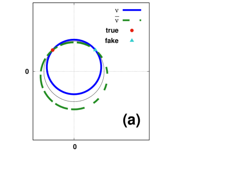
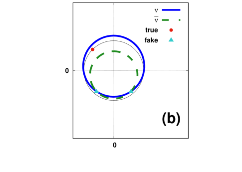
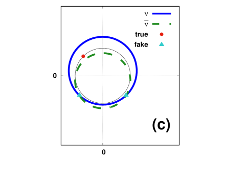
Figure 1: Determination of $\delta$ at T2HK using the complex plane of $z\equiv 2e^{-i\delta}s_{13}s_{23}$ in the case where the true value is $\delta^{\mbox{\tiny\rm true}}=5\pi/4$. The thick solid (dashed) circle stands for $P(\nu_{\mu}\to\nu_{e};\delta,\theta_{23})=P(\nu_{\mu}\to\nu_{e};\delta^{\mbox{\tiny\rm true}},\theta_{23}^{\mbox{\tiny\rm true}})$ ($P(\bar{\nu}_{\mu}\to\bar{\nu}_{e};\delta,\theta_{23})=P(\bar{\nu}_{\mu}\to\bar{\nu}_{e};\delta^{\mbox{\tiny\rm true}},\theta_{23}^{\mbox{\tiny\rm true}}$), while the thin solid circle stands for the circle with a radius $2s_{13}s_{23}$. (a): The case with the right octant ($\theta_{23}^{\mbox{\tiny\rm true}}=16\pi/60$, $\delta^{\mbox{\tiny\rm true}}=5\pi/4$). The true (fake) point $2\exp(-5i\pi/4)s_{13}s_{23}$ ($2\exp(-7i\pi/4)s_{13}s_{23}$) with $\delta=5\pi/4$ ($\delta=7\pi/4$) is depicted by a filled circle (a filled triangle). From the appearance channel, only $\sin\delta$ is determined, leaving the sign of $\cos\delta$ unknown. (b): The wrong octant $\theta_{23}=14\pi/60<\pi/4$ in the case where the true value $\theta_{23}^{\mbox{\tiny\rm true}}=16\pi/60$ is in the higher octant. (c): The wrong octant $\theta_{23}=16\pi/60>\pi/4$ in the case where the true value $\theta_{23}^{\mbox{\tiny\rm true}}=14\pi/60$ is in the lower octant. With the wrong octant, the solution for Eqs. (73) and (74) is inconsistent with the condition $|2e^{-i\delta}s_{13}s_{23}|=2s_{13}s_{23}$, i.e., the intersection of the two thick circles is not on the thin circle.

Here, for concreteness, we take the true values as $\delta^{\mbox{\tiny\rm true}}=5\pi/4$ and $\theta_{23}^{\mbox{\tiny\rm true}}=16\pi/60$ (with $(s_{23}^{\mbox{\tiny\rm true}})^{2}=0.552$) which are almost the best fit values at present [1], respectively. The problem of determining $\delta$ from the two equations

$$P\left(\nu_{\mu}\to\nu_{e};\delta,\theta_{23}=\frac{\pi}{4}\pm\frac{\pi}{60}\right)=P\left(\nu_{\mu}\to\nu_{e};\delta^{\mbox{\tiny\rm true}}=\frac{5}{4}\pi,\theta_{23}^{\mbox{\tiny\rm true}}=\frac{16}{60}\pi\right)$$ (73)

and

$$P\left(\bar{\nu}_{\mu}\to\bar{\nu}_{e};\delta,\theta_{23}=\frac{\pi}{4}\pm\frac{\pi}{60}\right)=P\left(\bar{\nu}_{\mu}\to\bar{\nu}_{e};\delta^{\mbox{\tiny\rm true}}=\frac{5}{4}\pi,\theta_{23}^{\mbox{\tiny\rm true}}=\frac{16}{60}\pi\right)$$ (74)

can be solved by looking for the intersection between the two circles in the complex plane of the variable $z\equiv 2\exp(-i\delta)s_{13}s_{23}$ as in Fig.1. Eq. (73) ((74)) tells us that the distance between the points $2\exp(-i\delta)s_{13}s_{23}$ and $-i(\pi/120)c_{23}\sin 2\theta_{12}$ ($i(\pi/120)c_{23}\sin 2\theta_{12}$) in the complex plane is the same as that between the points $2\exp(-5i\pi/4)s_{13}s_{23}$ and $i(\pi/120)c_{23}\sin 2\theta_{12}$ ($i(\pi/120)c_{23}\sin 2\theta_{12}$), respectively. If our hypothesis on the octant of $\theta_{23}$ is correct (in the present case it is in the higher octant ($\theta_{23}^{\mbox{\tiny\rm true}}=16\pi/60>\pi/4$)), then we have two solutions corresponding to $\cos\delta=\pm|\cos\delta|$, as is shown in Fig. 1 (a). On the other hand, if our hypothesis on the octant of $\theta_{23}$ is wrong, then the absolute value of the intersection points is not equal to $2s_{13}s_{23}$ (Fig. 1 (b) where a fit with $\theta_{23}=14\pi/60<\pi/4$ is attempted for the true value $\theta_{23}^{\mbox{\tiny\rm true}}=16\pi/60$) or (Fig. 1 (c) where a fit with $\theta_{23}=16\pi/60>\pi/4$ is attempted for the true value $\theta_{23}^{\mbox{\tiny\rm true}}=14\pi/60$), and we can reject the wrong hypotheses on the assumption that difference between the true and fake points is large enough compared with the experimental errors. Note that the precise value of $\theta_{13}$, which was determined by the reactor experiments [1], is crucial to resolve the octant degeneracy because it uniquely specifies the radius of the thin circle in Fig. 1.

To summarize so far, we have the following results from the T2HK data:

$\bullet$ For the sign degeneracy and the NSI parameters, we do not get any information.

$\bullet$ For the intrinsic degeneracy, we can determine the value of $\sin\delta$ but we still have ambiguity in the sign of $\cos\delta$.

$\bullet$ For the octant degeneracy, we can resolve it, on the assumption that deviation $|\pi/4-\theta_{23}|$ is large enough compared with the experimental errors.

Let us now turn to the appearance probabilities at T2HKK ($L$=1100km, 0.3GeV$\raisebox{0.85358pt}{\em$\,<$}\raisebox{-3.98337pt}{\em$\sim\,$}E\raisebox{0.85358pt}{\em$\,<$}\raisebox{-3.98337pt}{\em$\sim\,$}$ 1.1GeV). Since the T2HK appearance channel enables us to determine the value of $\sin\delta$ and the octant of $\theta_{23}$, we assume in the following discussions that we know the value of $\sin\delta$ and $\theta_{23}$, and the unknown are sign($\cos\delta$), sign($\Delta m_{31}^{2}$) and the NSI parameters. In the case of T2HKK, while $AL/2\,(\simeq 1/4)$ and $\Delta E_{21}L\,(\sim 0.2\,(0.6\mbox{\rm GeV}/E))$ can no longer be treated as small quantity, the term $U_{e3}U_{\mu 3}^{\ast}\epsilon_{D}$ in Eq. (LABEL:solarterm1) is of order $s_{13}^{2}$ from our assumption, so it can be ignored. Eq. (LABEL:solarterm1) contains the factor $\Delta\tilde{E}_{21}^{(\mp)}$ which is defined in Eq. (64), and it has the following expansion with respect to the small NSI parameters:

$$\Delta\tilde{E}_{21}^{(\mp)}\simeq\left.\Delta\tilde{E}_{21}^{(\mp)}\right|_{\mbox{\footnotesize\rm std}}+\delta\Delta\tilde{E}_{21}^{(\mp)}$$ (75)

$$\left.\Delta\tilde{E}_{21}^{(\mp)}\right|_{\mbox{\footnotesize\rm std}}\equiv\left\{\left(\Delta E_{21}\cos 2\theta_{12}\mp Ac_{13}^{2}\right)^{2}+\left(\Delta E_{21}\sin 2\theta_{12}\right)^{2}\right\}^{1/2}\,$$ (76)

$$\delta\Delta\tilde{E}_{21}^{(\mp)}\equiv\pm\frac{2A}{\left.\Delta\tilde{E}_{21}^{(\mp)}\right|_{\mbox{\footnotesize\rm std}}}\left\{\epsilon_{D}\left(\Delta E_{21}\cos 2\theta_{12}\mp Ac_{13}^{2}\right)+\mbox{\rm Re}(\epsilon_{N})\Delta E_{21}\sin 2\theta_{12}\right\}\,.$$ (77)

This small correction $\delta\Delta\tilde{E}_{21}^{(\mp)}$ also gives a contribution to the appearance probabilities, and we have

$$P(\nu_{\mu}\to\nu_{e})$$

$$\simeq\left|2U_{e3}U_{\mu 3}^{\ast}\sin\left(\frac{\Delta E_{31}L}{2}\right)+e^{i\Delta E_{31}L/2}\left\{\Delta E_{21}L\,U_{e2}U_{\mu 2}^{\ast}\right.\right.$$

$$\left.\left.+\left(\Delta E_{21}L-\left.\Delta\tilde{E}_{21}^{(-)}L\right|_{\epsilon_{\alpha\beta}=0}\right)\frac{U_{e3}U_{\mu 3}^{\ast}}{2}+AL\,U_{\tau 3}\epsilon_{N}\right\}\right|^{2}$$

$$\simeq\left|\Delta E_{21}L\,U_{e2}U_{\mu 2}^{\ast}+\left\{2e^{-i\Delta E_{31}L/2}\sin\left(\frac{\Delta E_{31}L}{2}\right)+\frac{\Delta E_{21}L}{2}-\left.\frac{\Delta\tilde{E}_{21}^{(-)}L}{2}\right|_{\epsilon_{\alpha\beta}=0}\right\}U_{e3}U_{\mu 3}^{\ast}\right.$$

$$\hskip 11.38109pt\left.+AL\,U_{\tau 3}\epsilon_{N}\right|^{2}$$

$$P(\bar{\nu}_{\mu}\to\bar{\nu}_{e})$$

$$\simeq\left|\Delta E_{21}L\,U_{e2}^{\ast}U_{\mu 2}+\left\{2e^{-i\Delta E_{31}L/2}\sin\left(\frac{\Delta E_{31}L}{2}\right)+\frac{\Delta E_{21}L}{2}-\left.\frac{\Delta\tilde{E}_{21}^{(+)}L}{2}\right|_{\epsilon_{\alpha\beta}=0}\right\}U_{e3}^{\ast}U_{\mu 3}\right.$$

$$\hskip 11.38109pt\left.-AL\,U_{\tau 3}\epsilon_{N}\right|^{2}$$ (79)

In the last equation in Eq. (4), the first line, which is assumed to be known up to the sign of $\cos\delta$, is the contribution of the standard three flavor framework and the second line is the NSI contribution. Assuming that $\delta$ is already known from the T2HK data (up to the sign of $\cos\delta$), the two equations

$$P(\nu_{\mu}\to\nu_{e};\epsilon_{N})=P(\nu_{\mu}\to\nu_{e};\epsilon_{N}^{\mbox{\tiny\rm true}})$$ (80)

and

$$P(\bar{\nu}_{\mu}\to\bar{\nu}_{e};\epsilon_{N})=P(\bar{\nu}_{\mu}\to\bar{\nu}_{e};\epsilon_{N}^{\mbox{\tiny\rm true}})$$ (81)

give us a condition on $\epsilon_{N}$.

A remark is in order. As was emphasized in Ref. [17], the reason that information on $\epsilon_{N}$ can be still obtained after expanding a sine function with a small argument as $\sin(\Delta\tilde{E}_{21}^{(\mp)}L/2)\simeq\Delta\tilde{E}_{21}^{(\mp)}L/2$ is because this is the case where a so-called vacuum mimicking phenomenon [30, 43, 44, 45, 46, 47, 48, 49] does not occur. In the standard three flavor framework, if the argument of a sine function is small and expanded as $\sin x\simeq x$, then the oscillation probability in matter is reduced to the one in vacuum, and this is call a vacuum mimicking phenomenon. In the present case, however, even after the approximation $\sin(\Delta\tilde{E}_{21}^{(\mp)}L/2)\simeq\Delta\tilde{E}_{21}^{(\mp)}L/2$ is used, the term with $\epsilon_{N}$ remains. This is an advantage of a long baseline experiment ($L\raisebox{0.85358pt}{\em$\,>$}\raisebox{-3.98337pt}{\em$\sim\,$}$1000km) at low energy ($E\raisebox{0.85358pt}{\em$\,<$}\raisebox{-3.98337pt}{\em$\sim\,$}$1GeV), such as T2HKK, since the other NSI parameters do not appear in the appearance probability to the leading order at low energy.

As in the case of T2HK, Eqs. (80) and (81) represent two circles in the complex plane of $z\equiv AL\,U_{\tau 3}\epsilon_{N}$, and in general there are two intersections. To reject the fake solutions, we need more information. We therefore consider the appearance probabilities at different three energy regions, e.g., $E$=0.3 GeV, $E$=0.7 GeV and $E$=1.1 GeV. Here we take $\epsilon_{N}^{\mbox{\tiny\rm true}}=0$ as the true value for simplicity. As we see in Fig. 2, there are four possible cases with right/wrong sign of $\cos\delta$ and right/wrong sign of $\Delta m_{31}^{2}$. By demanding that there be a common intersection point among the three pairs of circles, we can resolve degeneracy of sign($\sin\delta$) and that of sign($\Delta m_{31}^{2}$), and we can determine both Re($\epsilon_{N}$) and Im($\epsilon_{N}$), on the assumption that the difference between the true and fake points is large enough compared with the experimental errors. So far we have taken $\epsilon_{N}^{\mbox{\tiny\rm true}}=0$ as the true value for simplicity. If the true value $\epsilon_{N}^{\mbox{\tiny\rm true}}$ is nonzero, then the same argument can be applied, since all the positions of the circles and $\epsilon_{N}^{\mbox{\tiny\rm true}}$ in the complex plane are shifted by $\epsilon_{N}^{\mbox{\tiny\rm true}}\,(\neq 0$). Hence even for $\epsilon_{N}^{\mbox{\tiny\rm true}}\neq 0$, we can determine $\epsilon_{N}$ from the appearance probabilities of T2HKK and all the information from T2HK.

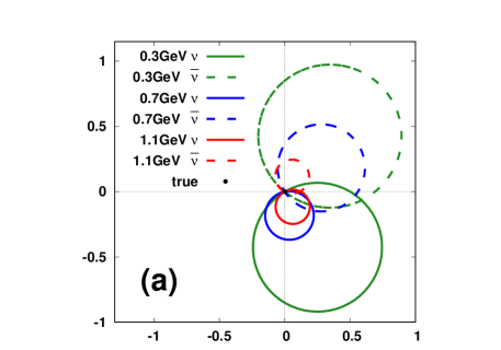
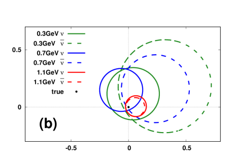
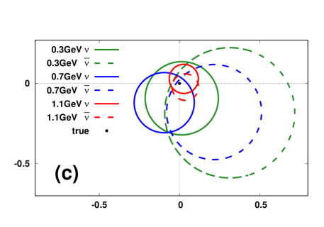
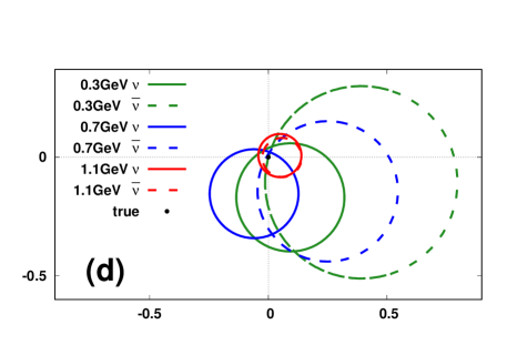
Figure 2: Four possible patterns at T2HKK in the complex plane of $z\equiv(AL/2)U_{\tau 3}\epsilon_{N}\simeq 0.18\,\epsilon_{N}$. The true solution can be selected by demanding that the three pairs of the circles has a common intersection. (a): a solution with choice of right sign($\sin\delta$) and right sign($\Delta m_{31}^{2}$). (b): a solution with choice of wrong sign($\sin\delta$) and right sign($\Delta m_{31}^{2}$). (c): a solution with choice of right sign($\sin\delta$) and wrong sign($\Delta m_{31}^{2}$). (d): a solution with choice of wrong sign($\sin\delta$) and wrong sign($\Delta m_{31}^{2}$).

Finally, let us discuss determination of $\epsilon_{D}$. In our approximation, $\epsilon_{D}$ does not appear in the appearance probabilities to the leading order. So far we have already determined $\delta$, $\theta_{23}$ and $\epsilon_{N}$, so we assume in the following discussions that we already know the value of these parameters. To get information on $\epsilon_{D}$, let us discuss the disappearance probabilities at T2HKK. They are given by (See Appendix C for details.)

$$\left\{\begin{array}[]{l}P(\nu_{\mu}\to\nu_{\mu})\\ P(\bar{\nu}_{\mu}\to\bar{\nu}_{\mu})\end{array}\right\}\simeq\left|AL\,\epsilon_{I}+f^{(\mp)}\epsilon_{D}+g^{(\mp)}\right|^{2}\,,$$ (84)

where $f^{(\mp)}=O(1)$ and $g^{(\mp)}=O(1)$ are defined by

$$f^{(\mp)}\equiv AL\left(c_{23}^{2}-i\frac{\Delta E_{21}\cos 2\theta_{12}\mp Ac_{13}^{2}}{\left.\Delta\tilde{E}_{21}^{(\mp)}\right|_{\mbox{\footnotesize\rm std}}}{\cal F}\right)$$

$$g^{(\mp)}\equiv\pm\exp\left(i\frac{L}{2}\left.\Delta\tilde{E}_{21}^{(\mp)}\right|_{\mbox{\tiny\rm std}}\right)\left\{\frac{i}{2}+e^{-i\Delta E_{31}L/2}|{U}_{\mu 3}|^{2}\sin\left(\frac{\Delta E_{31}L}{2}\right)\right\}$$

$$\pm\frac{\Delta E_{21}L}{2}|U_{\mu 2}|^{2}\pm\left(\frac{L}{2}\Delta E_{21}-\frac{L}{2}\left.\Delta\tilde{E}_{21}^{(\mp)}\right|_{\mbox{\tiny\rm std}}\right)\frac{|U_{\mu 3}|^{2}}{2}+\frac{AL}{2}\left(1+c_{23}^{2}\right)$$

$$-iAL\mbox{\rm Re}(\epsilon_{N})\frac{\Delta E_{21}\sin 2\theta_{12}}{\left.\Delta\tilde{E}_{21}^{(\mp)}\right|_{\mbox{\footnotesize\rm std}}}{\cal F}$$ (86)

with

$${\cal F}\equiv\frac{\Delta E_{21}L}{2}|U_{\mu 2}|^{2}+\left(\frac{L}{2}\Delta E_{21}-\frac{L}{2}\left.\Delta\tilde{E}_{21}^{(\mp)}\right|_{\mbox{\tiny\rm std}}-i\right)\frac{|U_{\mu 3}|^{2}}{2}\,.$$ (87)

From the discussions on the T2HK data and the appearance channel of T2HKK, we already know the values of $\delta$ and $\epsilon_{N}$. Assuming that the true values of the NSI parameters $\epsilon_{N}^{\mbox{\tiny\rm true}}$, $\epsilon_{I}^{\mbox{\tiny\rm true}}$ and $\epsilon_{D}^{\mbox{\tiny\rm true}}$ are zero for simplicity, the following equations give us information on $\epsilon_{I}$ and $\epsilon_{D}$:

$$P(\nu_{\mu}\to\nu_{\mu};\epsilon_{I},\epsilon_{D})=P(\nu_{\mu}\to\nu_{\mu};0,0)$$

$$\left|AL\,\epsilon_{I}+f^{(-)}\epsilon_{D}+g^{(-)}\right|^{2}=\left|g^{(-)}\right|^{2}$$

$$P(\bar{\nu}_{\mu}\to\bar{\nu}_{\mu};\epsilon_{I},\epsilon_{D})=P(\bar{\nu}_{\mu}\to\bar{\nu}_{\mu};0,0)$$

$$\left|AL\,\epsilon_{I}+f^{(+)}\epsilon_{D}+g^{(+)}\right|^{2}=\left|g^{(+)}\right|^{2}$$ (89)

Unlike in the case of the appearance probabilities, where the contributions from the atmospheric oscillation and from the solar one are both small, the NSI contributions in Eq. (LABEL:pmmv3) are small compared with the one from atmospheric oscillation. So we can expand the disappearance probabilities in term of the small parameters $\epsilon_{I}$ and $\epsilon_{D}$.

$$AL\,\mbox{\rm Re}\left[g^{(-)}\right]\,\epsilon_{I}+\mbox{\rm Re}\left[g^{(-)}f^{(-)\ast}\right]\,\epsilon_{D}=0$$ (90)

$$AL\,\mbox{\rm Re}\left[g^{(+)}\right]\,\epsilon_{I}+\mbox{\rm Re}\left[g^{(+)}f^{(+)\ast}\right]\,\epsilon_{D}=0$$ (91)

From these two equations we can determine $\epsilon_{I}$ and $\epsilon_{D}$. Here we have assumed that the true value of the NSI parameters are zero for simplicity, but even for a nonvanishing value of the NSI parameters, the same argument can be applied.

To summarize, we have seen that, because the T2HK experiment has a relatively short baseline length, the oscillation probabilities at T2HK are approximately independent of the NSI parameters and T2HK can determine the value of $\sin\delta$ and it can resolve the octant degeneracy, on the assumption that the difference between the true and fake points is large enough compared with the experimental errors. Furthermore, the T2HKK experiment can resolve degeneracy of the sign of $\Delta m_{31}^{2}$ as well as the ambiguity of $\cos\delta$. By combining the appearance and disappearance probabilities at T2HK and T2HKK, we can determine the NSI parameters $\epsilon_{N}$, $\epsilon_{I}$ and $\epsilon_{D}$.

5 Conclusions

At low energy ($E\raisebox{0.85358pt}{\em$\,<$}\raisebox{-3.98337pt}{\em$\sim\,$}$ 1GeV), the description in the solar flavor basis is useful. In particular, in the presence of the nonstandard interactions in propagation of neutrinos, assuming that the NSI parameters are at most of order O($s_{13}$), the appearance probabilities at low energy depend approximately only on one ($\epsilon_{N}$) of the NSI parameters, while the disappearance ones do on three (Re($\epsilon_{N}$), $\epsilon_{I}$ and $\epsilon_{D}$). Furthermore, assuming that the experimental errors are small enough to justify the analytical discussions on the oscillation probabilities, we discussed how parameter degeneracy can be resolved by combining the T2HK and T2HKK experiments. These two low energy long baseline experiments are complementary to each other, because T2HK has little sensitivity to the matter effect and can therefore determine $\sin\delta$ and the octant of $\theta_{23}$ without being disturbed by the existence of the NSI whereas T2HKK has sensitivity to the matter effect and can give us information on the NSI parameters as well as sign($\sin\delta$) and sign($\Delta m_{31}^{2}$). Our treatment in this work is qualitative in the sense that the experimental errors are not taken into account, and quantitative estimation of the experimental errors is beyond the scope of this work. Nevertheless, we hope that the present work sheds light on the advantage of low energy long baseline experiments to investigate the NSI which is suggested by the tension between the solar neutrino data and that from the KamLAND experiment.

Appendix A Analytical form of the oscillation probability and the Kimura-Takamura-Yokomakura formalism

If neutrino has a potential, which can in general has off diagonal components in the presence of the NSI, then the Hamiltonian in matter with constant density for neutrinos and antineutrinos can be formally diagonalized as

$$\left\{\begin{array}[]{l}U{\cal E}U^{-1}+{\cal A}\\ U^{\ast}{\cal E}(U^{\ast})^{-1}-{\cal A}\end{array}\right\}=\tilde{U}^{(\mp)}\tilde{{\cal E}}^{(\mp)}(\tilde{U}^{(\mp)})^{-1}\,.$$ (94)

In Eq. (94), ${\cal A}$ is the $3\times 3$ matrix of the matter potential defined in Eq. (8),

$${\cal E}\equiv{\mbox{\rm diag}}\left(0,\Delta E_{21},\Delta E_{31}\right)$$ (95)

with

$$\Delta E_{jk}\equiv E_{j}-E_{k}\simeq\frac{m_{j}^{2}-m_{k}^{2}}{2E}\equiv\frac{\Delta m_{jk}^{2}}{2E}$$ (96)

is the diagonal matrix with the energy eigenvalue of each mass eigenstate where the identity matrix times $E_{1}$ was subtracted without affecting the oscillation probability, and

$$\tilde{\cal E}^{(\mp)}\equiv{\mbox{\rm diag}}\left(\tilde{E}_{1}^{(\mp)},\tilde{E}_{2}^{(\mp)},\tilde{E}_{3}^{(\mp)}\right)$$ (97)

is the diagonal matrix with the energy eigenvalue in matter. From Eq. (94) one can obtain the oscillation probability

$$\left\{\begin{array}[]{l}P(\nu_{\alpha}\rightarrow\nu_{\beta})\\ P(\bar{\nu}_{\alpha}\rightarrow\bar{\nu}_{\beta})\end{array}\right\}$$

$$=\left|\sum_{j=1}^{3}\tilde{U}_{\beta j}^{(\mp)}\exp\left(-i\Delta\tilde{E}_{j1}^{(\mp)}L\right)\tilde{U}_{\alpha j}^{(\mp)^{\ast}}\right|^{2}$$

$$=\left|\delta_{\alpha\beta}-\sum_{j=1}^{3}\tilde{U}_{\beta j}^{(\mp)}\left\{1-\exp\left(-i\Delta\tilde{E}_{j1}^{(\mp)}L\right)\right\}\tilde{U}_{\alpha j}^{(\mp)^{\ast}}\right|^{2}$$

$$=\left|\delta_{\alpha\beta}-2i\exp\left(-\frac{i}{2}\Delta\tilde{E}_{j1}^{(\mp)}L\right)\sum_{j=2}^{3}\tilde{U}_{\beta j}^{(\mp)}\tilde{U}_{\alpha j}^{(\mp)^{\ast}}\sin\left(\frac{\Delta\tilde{E}_{j1}^{(\mp)}L}{2}\right)\right|^{2}\,,$$ (101)

where we have used the unitarity property $\sum_{j=1}^{3}\tilde{U}_{\beta j}^{(\mp)}\tilde{U}_{\alpha j}^{(\mp)^{\ast}}=\delta_{\alpha\beta}$ in the third line and we have defined

$$\Delta\tilde{E}_{jk}^{(\mp)}\equiv\tilde{E}_{j}^{(\mp)}-\tilde{E}_{k}^{(\mp)}\,.$$

Thus we can obtain the analytic expression if we get the bilinear form $\tilde{U}_{\beta j}^{(\mp)}\tilde{U}_{\alpha j}^{(\mp)^{\ast}}$.

It was shown by Kimura, Takamura and Yokomakura [36, 37] that $\tilde{U}_{\beta j}^{(\mp)}\tilde{U}_{\alpha j}^{(\mp)^{\ast}}$ can be expressed in terms of the known quantities as long as the energy eigenvalue $\tilde{E}_{j}^{(\mp)}$ is known. Their argument goes as follows. If we consider the ($\alpha$, $\beta$)-component of $n$-th power ($n=0,1,2$) of the neutrino part of Eq. (94), then we obtain

$$\delta_{\alpha\beta}=\left[\tilde{U}^{(-)}(\tilde{U}^{(-)})^{-1}\right]_{\alpha\beta}=\sum_{j}\tilde{U}_{\alpha j}^{(-)}(\tilde{U}_{\beta j}^{(-)})^{\ast}$$ (102)

$$\left[U{\cal E}U^{-1}+{\cal A}\right]_{\alpha\beta}=\left[\tilde{U}^{(-)}\tilde{{\cal E}^{(-)}}(\tilde{U}^{(-)})^{-1}\right]_{\alpha\beta}=\sum_{j}\tilde{E}_{j}^{(-)}\tilde{U}_{\alpha j}^{(-)}(\tilde{U}_{\beta j}^{(-)})^{\ast}$$ (103)

$$\left[\left(U{\cal E}U^{-1}+{\cal A}\right)^{2}\right]_{\alpha\beta}=\left[\tilde{U}^{(-)}\tilde{({\cal E}}^{(-)})^{2}\tilde{U}^{-1}\right]_{\alpha\beta}=\sum_{j}(\tilde{E}^{(-)}_{j})^{2}\tilde{U}_{\alpha j}^{(-)}(\tilde{U}_{\beta j}^{(-)})^{\ast}\,.$$ (104)

Putting Eqs. (102)–(104) together, we have

$$\left(\begin{array}[]{ccc}1&1&1\cr\tilde{E}_{1}^{(-)}&\tilde{E}_{2}^{(-)}&\tilde{E}_{3}^{(-)}\cr(\tilde{E}_{1}^{(-)})^{2}&(\tilde{E}_{2}^{(-)})^{2}&(\tilde{E}_{3}^{(-)})^{2}\end{array}\right)\left(\begin{array}[]{c}\tilde{U}_{\beta 1}^{(-)}\tilde{U}_{\alpha 1}^{(-)\ast}\cr\cr\tilde{U}_{\beta 2}^{(-)}\tilde{U}_{\alpha 2}^{(-)\ast}\cr\cr\tilde{U}_{\beta 3}^{(-)}\tilde{U}_{\alpha 3}^{(-)\ast}\end{array}\right)=\left(\begin{array}[]{r}\delta_{\alpha\beta}\cr\left[U{\cal E}U^{-1}+{\cal A}\right]_{\alpha\beta}\cr\left[\left(U{\cal E}U^{-1}+{\cal A}\right)^{2}\right]_{\alpha\beta}\end{array}\right),$$ (116)

which can be easily solved by inverting the Vandermonde matrix:

$$\left(\begin{array}[]{c}\tilde{U}_{\beta 1}^{(-)}\tilde{U}_{\alpha 1}^{(-)\ast}\cr\cr\tilde{U}_{\beta 2}^{(-)}\tilde{U}_{\alpha 2}^{(-)\ast}\cr\cr\tilde{U}_{\beta 3}^{(-)}\tilde{U}_{\alpha 3}^{(-)\ast}\end{array}\right)=\left(\begin{array}[]{ccc}\displaystyle\frac{{\ }1}{\Delta\tilde{E}_{21}^{(-)}\Delta\tilde{E}_{31}^{(-)}}(\tilde{E}_{2}^{(-)}\tilde{E}_{3}^{(-)},&-(\tilde{E}_{2}^{(-)}+\tilde{E}_{3}^{(-)}),&1)\cr\displaystyle\frac{-1}{\Delta\tilde{E}_{21}^{(-)}\Delta\tilde{E}_{32}^{(-)}}(\tilde{E}_{3}^{(-)}\tilde{E}_{1}^{(-)},&-(\tilde{E}_{3}^{(-)}+\tilde{E}_{1}^{(-)}),&1)\cr\displaystyle\frac{{\ }1}{\Delta\tilde{E}_{31}^{(-)}\Delta\tilde{E}_{32}^{(-)}}(\tilde{E}_{1}^{(-)}\tilde{E}_{2}^{(-)},&-(\tilde{E}_{1}^{(-)}+\tilde{E}_{2}^{(-)}),&1)\cr\end{array}\right)\left(\begin{array}[]{r}\delta_{\alpha\beta}\cr\cr\left[U{\cal E}U^{-1}+{\cal A}\right]_{\alpha\beta}\cr\cr\left[\left(U{\cal E}U^{-1}+{\cal A}\right)^{2}\right]_{\alpha\beta}\end{array}\right)\,.$$ (130)

The expression $\tilde{U}_{\beta j}^{(+)}\tilde{U}_{\alpha j}^{(+)\ast}$ for antineutrinos can be obtained in the same manner. Eq. (101) together with (LABEL:solx) is exact in the case with constant density of matter, as long as we know the energy eigenvalues $\tilde{E}_{j}^{(\mp)}$ exactly.

Appendix B The oscillation probabilities for $|\Delta m_{31}^{2}/2E|\gg A\sim\Delta m_{21}^{2}/2E$

In the case of low energy accelerator neutrinos, we have $|\Delta E_{31}|\equiv|\Delta m_{31}^{2}/2E|\gg A\simeq\Delta E_{21}\equiv\Delta m_{21}^{2}/2E$, so we keep $\Delta E_{31}$ and treat $A$ and $\Delta E_{21}$ as perturbation, keeping only terms of first order in $A$ and $\Delta E_{21}$.

The eigenvalues can be obtained from the eigenequation

$$0=\det(t\mbox{\bf 1}-M^{(\mp)})$$ (132)

$$=t^{3}-t^{2}\mbox{\rm Tr}[M^{(\mp)}]+\frac{t}{2}\left\{(\mbox{\rm Tr}[M^{(\mp)}])^{2}-\mbox{\rm Tr}[(M^{(\mp)})^{2}]\right\}$$

$$-\frac{1}{6}\left\{(\mbox{\rm Tr}[M^{(\mp)}])^{3}+2\mbox{\rm Tr}[(M^{(\mp)})^{3}]-3\mbox{\rm Tr}[M^{(\mp)}]\mbox{\rm Tr}[(M^{(\mp)})^{2}]\right\}\,.$$

Here the matrix can be expressed as

$$M^{(\mp)}\equiv\left\{\begin{array}[]{l}U{\cal E}U^{-1}{\cal A}=\Delta E_{31}U\eta_{3}U^{-1}+\Delta E_{21}U\eta_{2}U^{-1}+{\cal A}\\ U^{\ast}{\cal E}(U^{\ast})^{-1}-{\cal A}=\Delta E_{31}U^{\ast}\eta_{3}(U^{\ast})^{-1}+\Delta E_{21}U^{\ast}\eta_{2}(U^{\ast})^{-1}-{\cal A}\end{array}\right\}$$ (135)

where we have defined

$$\eta_{3}\equiv{\mbox{\rm diag}}\left(0,0,1\right)$$

$$\eta_{2}\equiv{\mbox{\rm diag}}\left(0,1,0\right)\,.$$

In the last equation in Eq. (135), the first term is large while the second and third terms are of order $\Delta m^{2}_{21}/|\Delta m^{2}_{31}|\simeq 1/30$. Applying a perturbation method with respect to $\Delta m^{2}_{21}/|\Delta m^{2}_{31}|$, we obtain the following eigenvalues for Eq. (132) to the leading order in $\Delta m^{2}_{21}/|\Delta m^{2}_{31}|$:

$$\left\{\begin{array}[]{l}\tilde{E}_{1}^{(\mp)}=\frac{1}{2}\left(\Delta E_{21}\pm\mbox{\rm Tr}[{\cal A}^{\prime}]\mp\mbox{\rm Tr}[\eta_{3}{\cal A}^{\prime}]-\Delta\tilde{E}_{21}^{(\mp)}\right)\\ \tilde{E}_{2}^{(\mp)}=\frac{1}{2}\left(\Delta E_{21}\pm\mbox{\rm Tr}[{\cal A}^{\prime}]\mp\mbox{\rm Tr}[\eta_{3}{\cal A}^{\prime}]+\Delta\tilde{E}_{21}^{(\mp)}\right)\\ \tilde{E}_{3}^{(\mp)}=\Delta E_{31}\pm\mbox{\rm Tr}[\eta_{3}{\cal A}^{\prime}]\,,\end{array}\right\}$$ (139)

where $\Delta\tilde{E}_{21}$ is defined by by Eq. (64). In obtaining Eq. (139), we have used the properties of hermitian matrices ${\cal A}$ and ${\cal A}^{\prime}\equiv\tilde{R}_{13}^{-1}\,R_{23}^{-1}\,{\cal A}\,R_{23}\,\tilde{R}_{13}$ which is defined in Eq. (37):

$$\mbox{\rm Tr}[{\cal A}]=\mbox{\rm Tr}[R_{23}\,\tilde{R}_{13}\,{\cal A}^{\prime}\,\tilde{R}_{13}^{-1}\,R_{23}^{-1}]=\mbox{\rm Tr}[{\cal A}^{\prime}]$$

$$\mbox{\rm Tr}[U\eta_{3}U^{-1}{\cal A}]=\mbox{\rm Tr}[\eta_{3}R_{12}^{-1}\,{\cal A}^{\prime}\,R_{12}]=\mbox{\rm Tr}[\eta_{3}{\cal A}^{\prime}]$$

$$\mbox{\rm Tr}[{\cal A}^{\ast}]=\mbox{\rm Tr}[({\cal A}^{\ast})^{T}]=\mbox{\rm Tr}[{\cal A}]$$

$$\mbox{\rm Tr}[({\cal A}^{\prime})^{\ast}]=\mbox{\rm Tr}[\{({\cal A}^{\prime})^{\ast}\}^{T}]=\mbox{\rm Tr}[{\cal A}^{\prime}]$$

$\tilde{E}_{3}^{(\mp)}$ in Eq. (139) is given to the next leading order in $\Delta m^{2}_{21}/|\Delta m^{2}_{31}|$ because it is necessary to obtain $\tilde{U}_{e2}^{(\mp)}\tilde{U}_{\mu 2}^{(\mp)\ast}$ later.

For simplicity, we obtain the bilinear form $\tilde{U}_{\beta j}^{(-)}\tilde{U}_{\alpha j}^{(-)\ast}$ for neutrinos only in the following. The one $\tilde{U}_{\beta j}^{(+)}\tilde{U}_{\alpha j}^{(+)\ast}$ for antineutrinos can be read off from the expression $\tilde{U}_{\beta j}^{(-)}\tilde{U}_{\alpha j}^{(-)\ast}$. Let us introduce the notation

$$Y_{j}^{\alpha\beta}\equiv\left[\left(U{\cal E}U^{-1}+{\cal A}\right)^{j-1}\right]_{\alpha\beta}$$

To perform perturbation calculations, it is convenient to rescale $\Delta E_{21}\to\epsilon\Delta E_{21}$ and ${\cal A}_{\alpha\beta}\to\epsilon{\cal A}_{\alpha\beta}$. Then we have

$$Y_{1}^{e\mu}=0$$

$$Y_{2}^{e\mu}=\left(U{\cal E}U^{-1}+{\cal A}\right)_{e\mu}$$

$$=\Delta E_{31}U_{e3}U_{\mu 3}^{\ast}+\epsilon\left(\Delta E_{21}U_{e2}U_{\mu 2}^{\ast}+{\cal A}_{e\mu}\right)$$

$$Y_{3}^{e\mu}=\left[\left(U{\cal E}U^{-1}+{\cal A}\right)^{2}\right]_{e\mu}$$

$$=\Delta E_{31}^{2}U_{e3}U_{\mu 3}^{\ast}+\epsilon\Delta E_{31}\{U\eta_{3}U^{-1},{\cal A}\}_{e\mu}$$

$$+\epsilon^{2}\left[\left(\Delta E_{21}\right)^{2}U_{e2}U_{\mu 2}^{\ast}+\Delta E_{21}U_{e2}U_{\mu 2}^{\ast}\{U\eta_{2}U^{-1},{\cal A}\}_{e\mu}+\left({\cal A}^{2}\right)_{e\mu}\right]$$

With these quantities, we have Eq. (58) to the leading order in ${\cal O}(\epsilon)$:

$$\tilde{U}_{e3}^{(-)}(\tilde{U}_{\mu 3}^{(-)})^{\ast}=\frac{-(\tilde{E}_{1}^{(-)}+\tilde{E}_{2}^{(-)})Y_{2}^{e\mu}+Y_{3}^{e\mu}}{(\tilde{E}_{3}^{(-)}-\tilde{E}_{1}^{(-)})(\tilde{E}_{3}^{(-)}-\tilde{E}_{2}^{(-)})}\simeq U_{e3}U_{\mu 3}^{\ast}\,.$$

In the case of antineutrinos, we have to replace $U_{\alpha j}$ by $U_{\alpha j}^{\ast}$, and we have Eq. (3.2)

$$\tilde{U}_{e3}^{(+)}(\tilde{U}_{\mu 3}^{(+)})^{\ast}\simeq U_{e3}^{\ast}U_{\mu 3}\,.$$

For $\tilde{U}_{e2}\tilde{U}_{\mu 2}^{\ast}$, we obtain Eq. (3.2) to the leading order in ${\cal O}(\epsilon)$:

$$\tilde{U}_{e2}^{(-)}\tilde{U}_{\mu 2}^{(-)\ast}=\frac{(\tilde{E}_{3}^{(-)}+\tilde{E}_{1}^{(-)})Y_{2}^{e\mu}-Y_{3}^{e\mu}}{(\tilde{E}_{3}^{(-)}-\tilde{E}_{2}^{(-)})(\tilde{E}_{2}^{(-)}-\tilde{E}_{1}^{(-)})}$$

$$\hskip 14.22636pt\simeq\frac{1}{\Delta\tilde{E}_{21}^{(-)}}\left\{\Delta E_{21}U_{e2}U_{\mu 2}^{\ast}+\left(\Delta E_{21}-\Delta\tilde{E}_{21}^{(-)}\right)\frac{U_{e3}U_{\mu 3}^{\ast}}{2}\right\}$$

$$\hskip 19.91692pt+\frac{1}{\Delta\tilde{E}_{21}^{(-)}}\left[{\cal A}_{e\mu}-\{U\eta_{3}U^{-1},{\cal A}\}_{e\mu}+\left(\mbox{\rm Tr}[{\cal A}]+\mbox{\rm Tr}[U\eta_{3}U^{-1}{\cal A}]\right)\frac{U_{e3}U_{\mu 3}^{\ast}}{2}\right]$$

$$\hskip 14.22636pt\simeq\frac{1}{\Delta\tilde{E}_{21}^{(-)}}\left[\Delta E_{21}U_{e2}U_{\mu 2}^{\ast}+\left\{\Delta E_{21}-\Delta\tilde{E}_{21}^{(-)}+A\left(2\epsilon_{D}-c_{13}^{2}\right)\right\}\frac{U_{e3}U_{\mu 3}^{\ast}}{2}+A\epsilon_{N}U_{\tau 3}\right]$$

$\epsilon_{I}$, $\epsilon_{D}$ and $\epsilon_{N}$ are defined in Eqs. (65), (66) and (67). In the case of antineutrinos, we have to replace $U_{\alpha j}$ by $U_{\alpha j}^{\ast}$ and ${\cal A}$ by $-{\cal A}$, and we have Eq. (61)

$$\tilde{U}_{e2}^{(+)}(\tilde{U}_{\mu 2}^{(+)})^{\ast}\simeq\frac{1}{\Delta\tilde{E}_{21}^{(-)}}\left[\Delta E_{21}U_{e2}^{\ast}U_{\mu 2}+\left\{\Delta E_{21}-\Delta\tilde{E}_{21}^{(-)}-A\left(2\epsilon_{D}-c_{13}^{2}\right)\right\}\frac{U_{e3}^{\ast}U_{\mu 3}}{2}-A\epsilon_{N}U_{\tau 3}\right]\,.$$

As for the disappearance channel, on the other hand, we have the following:

$$Y_{1}^{\mu\mu}=1$$

$$Y_{2}^{\mu\mu}=\left(U{\cal E}U^{-1}+{\cal A}\right)_{\mu\mu}$$

$$=\Delta E_{31}|U_{\mu 3}|^{2}+\epsilon\left(\Delta E_{21}|U_{\mu 2}|^{2}+{\cal A}_{\mu\mu}\right)$$

$$Y_{3}^{\mu\mu}=\left\{\left(U{\cal E}U^{-1}+{\cal A}\right)\right\}_{\mu\mu}$$

$$=\Delta E_{31}^{2}|U_{\mu 3}|^{2}+\epsilon\Delta E_{31}\{U\eta_{3}U^{-1},{\cal A}\}_{\mu\mu}$$

$$+\epsilon^{2}\left[\left(\Delta E_{21}\right)^{2}|U_{\mu 2}|^{2}+\Delta E_{21}|U_{\mu 2}|^{2}\{U\eta_{2}U^{-1},{\cal A}\}_{\mu\mu}+\left({\cal A}^{2}\right)_{\mu\mu}\right]$$

The bilinear form $|\tilde{U}_{\mu 3}^{(-)}|^{2}$ is thus given by Eq. (3.2):

$$|\tilde{U}_{\mu 3}^{(-)}|^{2}=\frac{-(\tilde{E}_{1}^{(-)}+\tilde{E}_{2}^{(-)})Y_{2}^{\mu\mu}+Y_{3}^{\mu\mu}}{(\tilde{E}_{3}^{(-)}-\tilde{E}_{1}^{(-)})(\tilde{E}_{3}^{(-)}-\tilde{E}_{2}^{(-)})}\simeq|U_{\mu 3}|^{2}\,.$$

$|\tilde{U}_{\mu 3}^{(+)}|^{2}$ is also equal to the one in vacuum and therefore is given by Eq. (3.2). $|\tilde{U}_{\mu 2}^{(-)}|^{2}$ is given by Eq. (63):

$$|\tilde{U}_{\mu 2}^{(-)}|^{2}=-\frac{\tilde{E}_{3}^{(-)}\tilde{E}_{1}^{(-)}-(\tilde{E}_{3}^{(-)}+\tilde{E}_{1}^{(-)})Y_{2}^{\mu\mu}+Y_{3}^{\mu\mu}}{(\tilde{E}_{3}^{(-)}-\tilde{E}_{1}^{(-)})(\tilde{E}_{2}^{(-)}-\tilde{E}_{1}^{(-)})}$$

$$\simeq\frac{1}{\Delta\tilde{E}_{21}^{(-)}}\left\{\Delta E_{21}|U_{\mu 2}|^{2}+\left(\Delta E_{21}-\Delta\tilde{E}_{21}^{(-)}\right)\frac{|U_{\mu 3}|^{2}}{2}\right\}$$

$$+\frac{1}{\Delta\tilde{E}_{21}^{(-)}}\left[{\cal A}_{\mu\mu}-\{U\eta_{3}U^{-1},{\cal A}\}_{\mu\mu}+\left(\mbox{\rm Tr}[{\cal A}]+\mbox{\rm Tr}[U\eta_{3}U^{-1}{\cal A}]\right)\frac{|U_{\mu 3}|^{2}}{2}\right]$$

$$\simeq\frac{1}{\Delta\tilde{E}_{21}^{(-)}}\left[\Delta E_{21}|U_{\mu 2}|^{2}+\left(\Delta E_{21}-\Delta\tilde{E}_{21}^{(-)}\right)\frac{|U_{\mu 3}|^{2}}{2}\right.+A\left(1+c_{23}^{2}\right)$$

$$\hskip 28.45274pt\left.+2A\,\left(\epsilon_{I}-\epsilon_{D}\,c_{23}^{2}\right)\right]$$

In the case of antineutrinos, we have to replace ${\cal A}$ by $-{\cal A}$, so we get

$$|\tilde{U}_{\mu 2}^{(+)}|^{2}\simeq\frac{1}{\Delta\tilde{E}_{21}^{(+)}}\left[\Delta E_{21}|U_{\mu 2}|^{2}+\left(\Delta E_{21}-\Delta\tilde{E}_{21}^{(+)}\right)\frac{|U_{\mu 3}|^{2}}{2}\right.-A\left(1+c_{23}^{2}\right)$$

$$\hskip 28.45274pt\left.-2A\,\left(\epsilon_{I}-\epsilon_{D}\,c_{23}^{2}\right)\right]$$

as in Eq. (63).

Appendix C Derivation of $f^{(\mp)}$ in (4) and $g^{(\mp)}$ in (86)

From Eq. (LABEL:pmm), using Eqs. (3.2), (63), and (75)–(77), we have

$$\left\{\begin{array}[]{l}P(\nu_{\mu}\to\nu_{\mu})\\ P(\bar{\nu}_{\mu}\to\bar{\nu}_{\mu})\end{array}\right\}$$

$$\simeq\left|1-2ie^{-i\Delta E_{31}L/2}|{U}_{\mu 3}|^{2}\sin\left(\frac{\Delta E_{31}L}{2}\right)-2i\exp\left(-i\frac{L}{2}\left.\Delta\tilde{E}_{21}^{(\mp)}\right|_{\mbox{\tiny\rm std}}\right)e^{-i\delta\Delta\tilde{E}_{21}^{(\mp)}L/2}|\tilde{U}_{\mu 2}^{(\mp)}|^{2}\frac{\Delta\tilde{E}_{21}^{(\mp)}L}{2}\right|^{2}$$

$$=4\left|\exp\left(i\frac{L}{2}\left.\Delta\tilde{E}_{21}^{(\mp)}\right|_{\mbox{\tiny\rm std}}\right)\left\{\frac{i}{2}+e^{-i\Delta E_{31}L/2}|{U}_{\mu 3}|^{2}\sin\left(\frac{\Delta E_{31}L}{2}\right)\right\}+e^{-i\delta\Delta\tilde{E}_{21}^{(\mp)}L/2}|\tilde{U}_{\mu 2}^{(\mp)}|^{2}\frac{\Delta\tilde{E}_{21}^{(\mp)}L}{2}\right|^{2}$$

$$\simeq 4\left|\exp\left(i\frac{L}{2}\left.\Delta\tilde{E}_{21}^{(\mp)}\right|_{\mbox{\tiny\rm std}}\right)\left\{\frac{i}{2}+e^{-i\Delta E_{31}L/2}|{U}_{\mu 3}|^{2}\sin\left(\frac{\Delta E_{31}L}{2}\right)\right\}\right.$$

$$+\left(1-i\frac{L}{2}\delta\Delta\tilde{E}_{21}^{(\mp)}\right)\left[\frac{\Delta E_{21}L}{2}|U_{\mu 2}|^{2}+\left(\frac{\Delta E_{21}L}{2}-\frac{\left.\Delta\tilde{E}_{21}^{(\mp)}\right|_{\mbox{\tiny\rm std}}L+\delta\Delta\tilde{E}_{21}^{(\mp)}L}{2}\right)\frac{|U_{\mu 3}|^{2}}{2}\right.$$

$$\hskip 99.58464pt\left.\pm\frac{AL}{2}\left(1+c_{23}^{2}+2\,\epsilon_{I}+2\,\epsilon_{D}\left.c_{23}^{2}\right)\right]\right|^{2}$$

$$\simeq 4\left|\exp\left(i\frac{L}{2}\left.\Delta\tilde{E}_{21}^{(\mp)}\right|_{\mbox{\tiny\rm std}}\right)\left\{\frac{i}{2}+e^{-i\Delta E_{31}L/2}|{U}_{\mu 3}|^{2}\sin\left(\frac{\Delta E_{31}L}{2}\right)\right\}\right.$$

$$+\frac{\Delta E_{21}L}{2}|U_{\mu 2}|^{2}+\left(\frac{L}{2}\Delta E_{21}-\frac{L}{2}\left.\Delta\tilde{E}_{21}^{(\mp)}\right|_{\mbox{\tiny\rm std}}\right)\frac{|U_{\mu 3}|^{2}}{2}\pm\frac{AL}{2}\left(1+c_{23}^{2}\right)$$

$$-i\frac{L}{2}\delta\Delta\tilde{E}_{21}^{(\mp)}\left\{\frac{\Delta E_{21}L}{2}|U_{\mu 2}|^{2}+\left(\frac{L}{2}\Delta E_{21}-\frac{L}{2}\left.\Delta\tilde{E}_{21}^{(\mp)}\right|_{\mbox{\tiny\rm std}}-i\right)\frac{|U_{\mu 3}|^{2}}{2}\right\}$$

$$\pm AL\left(\,\epsilon_{I}+\,\epsilon_{D}\left.c_{23}^{2}\right)\right|^{2}\,,$$

where Eq. (4) was used in the third step above. Here introducing the notation

$${\cal F}\equiv\frac{\Delta E_{21}L}{2}|U_{\mu 2}|^{2}+\left(\frac{L}{2}\Delta E_{21}-\frac{L}{2}\left.\Delta\tilde{E}_{21}^{(\mp)}\right|_{\mbox{\tiny\rm std}}-i\right)\frac{|U_{\mu 3}|^{2}}{2}$$

as in Eq. (87), we get

$$\left\{\begin{array}[]{l}P(\nu_{\mu}\to\nu_{\mu})\\ P(\bar{\nu}_{\mu}\to\bar{\nu}_{\mu})\end{array}\right\}$$

$$\simeq 4\left|\exp\left(i\frac{L}{2}\left.\Delta\tilde{E}_{21}^{(\mp)}\right|_{\mbox{\tiny\rm std}}\right)\left\{\frac{i}{2}+e^{-i\Delta E_{31}L/2}|{U}_{\mu 3}|^{2}\sin\left(\frac{\Delta E_{31}L}{2}\right)\right\}\right.$$

$$+\frac{\Delta E_{21}L}{2}|U_{\mu 2}|^{2}+\left(\frac{L}{2}\Delta E_{21}-\frac{L}{2}\left.\Delta\tilde{E}_{21}^{(\mp)}\right|_{\mbox{\tiny\rm std}}\right)\frac{|U_{\mu 3}|^{2}}{2}\pm\frac{AL}{2}\left(1+c_{23}^{2}\right)$$

$$\mp i\frac{AL}{\left.\Delta\tilde{E}_{21}^{(\mp)}\right|_{\mbox{\footnotesize\rm std}}}\left\{\epsilon_{D}\left(\Delta E_{21}\cos 2\theta_{12}\mp Ac_{13}^{2}\right)+\mbox{\rm Re}(\epsilon_{N})\Delta E_{21}\sin 2\theta_{12}\right\}\,{\cal F}$$

$$\pm AL\left(\,\epsilon_{I}+\,\epsilon_{D}\left.c_{23}^{2}\right)\right|^{2}$$

$$=4\left|\exp\left(i\frac{L}{2}\left.\Delta\tilde{E}_{21}^{(\mp)}\right|_{\mbox{\tiny\rm std}}\right)\left\{\frac{i}{2}+e^{-i\Delta E_{31}L/2}|{U}_{\mu 3}|^{2}\sin\left(\frac{\Delta E_{31}L}{2}\right)\right\}\right.$$

$$+\frac{\Delta E_{21}L}{2}|U_{\mu 2}|^{2}+\left(\frac{L}{2}\Delta E_{21}-\frac{L}{2}\left.\Delta\tilde{E}_{21}^{(\mp)}\right|_{\mbox{\tiny\rm std}}\right)\frac{|U_{\mu 3}|^{2}}{2}\pm\frac{AL}{2}\left(1+c_{23}^{2}\right)$$

$$\left.\pm AL\left[\,\epsilon_{I}+\,\epsilon_{D}\left(c_{23}^{2}-i\frac{\Delta E_{21}\cos 2\theta_{12}\mp Ac_{13}^{2}}{\left.\Delta\tilde{E}_{21}^{(\mp)}\right|_{\mbox{\footnotesize\rm std}}}{\cal F}\right)-i\mbox{\rm Re}(\epsilon_{N})\frac{\Delta E_{21}\sin 2\theta_{12}}{\left.\Delta\tilde{E}_{21}^{(\mp)}\right|_{\mbox{\footnotesize\rm std}}}{\cal F}\right]\right|^{2}$$

Thus we get the expressions (4) for $f^{(\mp)}$ and (86) for $g^{(\mp)}$.

References

[1]
M. Tanabashi et al. [Particle Data Group],
Phys. Rev. D 98 (2018) no.3, 030001.
doi:10.1103/PhysRevD.98.030001
[2]
F. Capozzi, E. Lisi, A. Marrone and A. Palazzo,
Prog. Part. Nucl. Phys. 102 (2018) 48
doi:10.1016/j.ppnp.2018.05.005
[arXiv:1804.09678 [hep-ph]].
[3]
I. Esteban, M. C. Gonzalez-Garcia, A. Hernandez-Cabezudo, M. Maltoni and T. Schwetz,
JHEP 1901 (2019) 106
doi:10.1007/JHEP01(2019)106
[arXiv:1811.05487 [hep-ph]].
[4]
J. W. F. Valle,
PoS NOW 2018 (2019) 022
doi:10.22323/1.337.0022
[arXiv:1812.07945 [hep-ph]].
[5]
K. Abe et al. [Hyper-Kamiokande Working Group],
arXiv:1412.4673 [physics.ins-det].
[6]
K. Abe et al. [Hyper-Kamiokande Collaboration],
PTEP 2018 (2018) no.6, 063C01
doi:10.1093/ptep/pty044
[arXiv:1611.06118 [hep-ex]].
[7]
R. Acciarri et al. [DUNE Collaboration],
arXiv:1512.06148 [physics.ins-det].
[8]
M. C. Gonzalez-Garcia and M. Maltoni,
JHEP 1309 (2013) 152
doi:10.1007/JHEP09(2013)152
[arXiv:1307.3092 [hep-ph]].
[9]
I. Esteban, M. C. Gonzalez-Garcia, M. Maltoni, I. Martinez-Soler and J. Salvado,
JHEP 1808 (2018) 180
doi:10.1007/JHEP08(2018)180
[arXiv:1805.04530 [hep-ph]].
[10]
M. Maltoni and A. Y. Smirnov,
Eur. Phys. J. A 52 (2016) no.4, 87
doi:10.1140/epja/i2016-16087-0
[arXiv:1507.05287 [hep-ph]].
[12]
O. G. Miranda and H. Nunokawa,
New J. Phys. 17 (2015) no.9, 095002
doi:10.1088/1367-2630/17/9/095002
[arXiv:1505.06254 [hep-ph]].
[13]
P. S. Bhupal Dev et al.,
SciPost Phys. Proc. 2 (2019) 001
doi:10.21468/SciPostPhysProc.2.001
[arXiv:1907.00991 [hep-ph]].
[14]
K. N. Abazajian et al.,
arXiv:1204.5379 [hep-ph].
[15]
S. Fukasawa and O. Yasuda,
Nucl. Phys. B 914 (2017) 99
doi:10.1016/j.nuclphysb.2016.11.004
[arXiv:1608.05897 [hep-ph]].
[16]
M. Ghosh and O. Yasuda,
arXiv:1709.08264 [hep-ph].
[17]
S. F. Ge and A. Y. Smirnov,
JHEP 1610 (2016) 138
doi:10.1007/JHEP10(2016)138
[arXiv:1607.08513 [hep-ph]].
[18]
A. M. Gago, H. Minakata, H. Nunokawa, S. Uchinami and R. Zukanovich Funchal,
JHEP 1001 (2010) 049
doi:10.1007/JHEP01(2010)049
[arXiv:0904.3360 [hep-ph]].
[19]
P. Coloma, A. Donini, J. Lopez-Pavon and H. Minakata,
JHEP 1108 (2011) 036
doi:10.1007/JHEP08(2011)036
[arXiv:1105.5936 [hep-ph]].
[20]
P. Bakhti and Y. Farzan,
JHEP 1407 (2014) 064
doi:10.1007/JHEP07(2014)064
[arXiv:1403.0744 [hep-ph]].
[21]
I. Mocioiu and W. Wright,
Nucl. Phys. B 893 (2015) 376
doi:10.1016/j.nuclphysb.2015.02.016
[arXiv:1410.6193 [hep-ph]].
[22]
P. Coloma,
JHEP 1603 (2016) 016
doi:10.1007/JHEP03(2016)016
[arXiv:1511.06357 [hep-ph]].
[23]
J. Liao, D. Marfatia and K. Whisnant,
Phys. Rev. D 93 (2016) no.9, 093016
doi:10.1103/PhysRevD.93.093016
[arXiv:1601.00927 [hep-ph]].
[24]
M. Blennow, S. Choubey, T. Ohlsson, D. Pramanik and S. K. Raut,
JHEP 1608 (2016) 090
doi:10.1007/JHEP08(2016)090
[arXiv:1606.08851 [hep-ph]].
[25]
S. K. Agarwalla, S. S. Chatterjee and A. Palazzo,
Phys. Lett. B 762 (2016) 64
doi:10.1016/j.physletb.2016.09.020
[arXiv:1607.01745 [hep-ph]].
[26]
K. N. Deepthi, S. Goswami and N. Nath,
Phys. Rev. D 96 (2017) no.7, 075023
doi:10.1103/PhysRevD.96.075023
[arXiv:1612.00784 [hep-ph]].
[27]
J. Liao, D. Marfatia and K. Whisnant,
JHEP 1701 (2017) 071
doi:10.1007/JHEP01(2017)071
[arXiv:1612.01443 [hep-ph]].
[28]
M. Masud, S. Roy and P. Mehta,
Phys. Rev. D 99 (2019) no.11, 115032
doi:10.1103/PhysRevD.99.115032
[arXiv:1812.10290 [hep-ph]].
[29]
S. Verma and S. Bhardwaj,
Adv. High Energy Phys. 2019 (2019) 8464535.
doi:10.1155/2019/8464535
[30]
L. Wolfenstein,
Phys. Rev. D 17 (1978) 2369.
doi:10.1103/PhysRevD.17.2369
[31]
J. W. F. Valle,
Phys. Lett. B 199 (1987) 432.
doi:10.1016/0370-2693(87)90947-6
[32]
M. M. Guzzo, A. Masiero and S. T. Petcov,
Phys. Lett. B 260 (1991) 154.
doi:10.1016/0370-2693(91)90984-X
[33]
E. Roulet,
Phys. Rev. D 44 (1991) R935.
doi:10.1103/PhysRevD.44.R935
[34]
S. Davidson, C. Pena-Garay, N. Rius and A. Santamaria,
JHEP 0303 (2003) 011
doi:10.1088/1126-6708/2003/03/011
[hep-ph/0302093].
[35]
C. Biggio, M. Blennow and E. Fernandez-Martinez,
JHEP 0908, 090 (2009)
doi:10.1088/1126-6708/2009/08/090
[arXiv:0907.0097 [hep-ph]].
[36]
K. Kimura, A. Takamura and H. Yokomakura,
Phys. Lett. B 537 (2002) 86
doi:10.1016/S0370-2693(02)01907-X
[hep-ph/0203099].
[37]
K. Kimura, A. Takamura and H. Yokomakura,
Phys. Rev. D 66 (2002) 073005
doi:10.1103/PhysRevD.66.073005
[hep-ph/0205295].
[38]
J. Burguet-Castell, M. B. Gavela, J. J. Gomez-Cadenas, P. Hernandez and O. Mena,
Nucl. Phys. B 608 (2001) 301
doi:10.1016/S0550-3213(01)00248-6
[hep-ph/0103258].
[39]
H. Minakata and H. Nunokawa,
JHEP 0110 (2001) 001
doi:10.1088/1126-6708/2001/10/001
[hep-ph/0108085].
[40]
G. L. Fogli and E. Lisi,
Phys. Rev. D 54 (1996) 3667
doi:10.1103/PhysRevD.54.3667
[hep-ph/9604415].
[41]
V. Barger, D. Marfatia and K. Whisnant,
Phys. Rev. D 65 (2002) 073023
doi:10.1103/PhysRevD.65.073023
[hep-ph/0112119].
[42]
Y. Itow et al. [T2K Collaboration],
hep-ex/0106019.
[43]
A. De Rujula, M. B. Gavela and P. Hernandez,
Nucl. Phys. B 547 (1999) 21
doi:10.1016/S0550-3213(99)00070-X
[hep-ph/9811390].
[44]
M. Freund, M. Lindner, S. T. Petcov and A. Romanino,
Nucl. Phys. B 578 (2000) 27
doi:10.1016/S0550-3213(00)00179-6
[hep-ph/9912457].
[45]
E. K. Akhmedov,
Phys. Lett. B 503 (2001) 133
doi:10.1016/S0370-2693(01)00165-4
[hep-ph/0011136].
[46]
P. Lipari,
Phys. Rev. D 64 (2001) 033002
doi:10.1103/PhysRevD.64.033002
[hep-ph/0102046].
[47]
H. Minakata and H. Nunokawa,
Phys. Lett. B 495 (2000) 369
doi:10.1016/S0370-2693(00)01249-1
[hep-ph/0004114].
[48]
H. Minakata,
Nucl. Phys. Proc. Suppl. 100 (2001) 237
doi:10.1016/S0920-5632(01)01447-5
[hep-ph/0101231].
[49]
O. Yasuda,
Phys. Lett. B 516 (2001) 111
doi:10.1016/S0370-2693(01)00920-0
[hep-ph/0106232].