Transition to classical regime in quantum mechanics on a lattice
and implications of discontinuous space

Abstract

It is well known that due to the uncertainty principle the Planck constant sets a resolution boundary in phase space and the resulting trade-off in resolutions between incompatible measurements has been thoroughly investigated. It is also known that in the classical regime sufficiently coarse measurements of position and momentum can simultaneously be determined. However, the picture of how the uncertainty principle gradually disappears as we transition from the quantum to the classical regime is not so vivid. In the present work we will clarify this picture by studying the associated probabilities that quantify the effects of the uncertainty principle in the framework of finite-dimensional quantum mechanics on a lattice. We will also study how these probabilities are perturbed by the granularity of the lattice and show that they can signal the discontinuity of the underlying space.

I Introduction

Heisenberg’s uncertainty principle is colloquially understood as the fact that arbitrarily precise values of position and momentum cannot simultaneously be determined (see (Busch and Shilladay, 2006; Busch et al., 2007) for a review). A rigorous formulation of the uncertainty principle is often conflated with the uncertainty relations for states $\sigma_{x}\sigma_{p}\geq\hbar/2$, where $\sigma_{x}$ and $\sigma_{p}$ refer to the standard deviations of independently measured position and momentum of a particle in the same state. This inequality is also known as preparation uncertainty relations because it rules out the possibility of preparing quantum states with arbitrarily sharp values of both position and moment. It does not, however, rule out the possibility of measurements that simultaneously determine both of these values with arbitrary precision. The essential effect that rules out the latter possibility is the mutual disturbance between measurements of incompatible observables, also known as error-disturbance uncertainty relations.

According to the original formulation by Heisenberg (Heisenberg, 1927), due to the unavoidable disturbance by measurements, it is not possible to localize a particle in a phase space cell of the size of the Planck constant or smaller. However, when phase space cells much coarser than the Planck constant are considered, Heisenberg argued that the values of both observables can be estimated at the expense of lower resolution. The picture that emerges from Heisenberg’s original arguments is that the Planck constant sets a resolution boundary in phase space (see Fig. 1 left) that separates the quantum scale from the classical scale. There is, of course, a continuum of scales and it is natural to ask for a characteristic function that outlines how the uncertainty principle becomes inconsequential as we decrease the resolution of measurements.

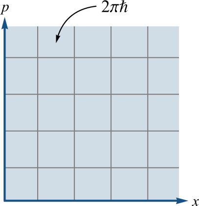
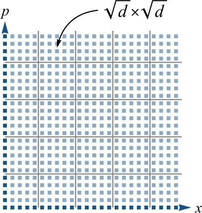
Figure 1: (left) The continuous phase space where the cells with the area $2\pi\hbar$ represent the resolution scale associated with the uncertainty principle. (right) The discretized phase space of a lattice of integer length $d$. Analogous cells with the area $\sqrt{d}\times\sqrt{d}$ arise from the scale $\sqrt{d}$ which is the geometric mean of the minimal length ($1$) and the maximal length ($d$) on a unitless lattice. The Planck constant $2\pi\hbar$ can be recovered from $\sqrt{d}$ by converting the phase space area $\sqrt{d}\times\sqrt{d}$ to proper units.

A rigorous formulation of the error-disturbance uncertainty relations has been extensively debated in recent years (Ozawa, 2003; Busch et al., 2013; Branciard, 2013; Korzekwa et al., 2014; Buscemi et al., 2014; Rozema et al., 2015), producing multiple perspectives on the fundamental limits of simultaneous measurability of incompatible observables. These formulations are similar to the preparation uncertainty relations as they capture the trade-off between the resolution and disturbance of measurements (which may also depend on the states). However, the error-disturbance relations focus on the limits of simultaneous measurability but they do not outline how the mutual disturbance effects fade away with decreasing resolution of measurements.

In the present work we will study the mutual disturbance effects of the uncertainty principle on a finite-dimensional lattice of integer length $d$. We will quantify the mutual disturbance effects with the average probability $\left\langle\boldsymbol{p}_{\textrm{agree}}\right\rangle$ that an instantaneous succession of coarse-grained measurements of position-momentum-position will agree on both outcomes of position. Since the value $\left\langle\boldsymbol{p}_{\textrm{agree}}\right\rangle$ measures the strength of the mutual disturbance effects as a function of measurement resolution, it will allow us to quantitatively outline the transition from the quantum to the classical regime where the mutual disturbance effects fade away. With that we will show that the geometric mean of the minimal length and the maximal length on a lattice is a significant scale that separates the classical regime of joint measurability, from the quantum regime where mutual disturbance effects are important (see Fig. 1 right).

The idea of using coarse-grained measurements to study the quantum-to-classical transitions is not new. Most notably (and what initially inspired this work) is the work of Asher Peres (Peres, 2006), and later of Kofler and Brukner (Kofler and Brukner, 2007), where it was argued that classical physics arises from sufficiently coarse measurements. This idea has also been investigated from the perspectives of entanglement observability (Raeisi et al., 2011) and Bell’s or Leggett-Garg inequalities (Jeong et al., 2014). There are also a series of studies by Rudnicki et al (Rudnicki et al., 2012a, b; Toscano et al., 2018) on uncertainty relations for coarse-grained observables. What is different about the present work is that we do not focus on the limits captured by a certain bound (as in Bell’s inequalities or uncertainty relations) but on the average case captured by the probability $\left\langle\boldsymbol{p}_{\textrm{agree}}\right\rangle$.

Our analysis of the mutual disturbance effects on a lattice with discretized lengths are also related to what is known as the generalized uncertainty principle (Ali et al., 2009). The idea of the generalized uncertainty principle follows from the fact that the continuous phase space picture is incompatible with the various approaches to quantum gravity (Hossenfelder, 2013) where the minimal resolvable length is $\delta x\sim 10^{-35}\,\textrm{m}$. The existence of such minimal length should affect the uncertainty principle and it is usually captured by modifying the canonical commutation relations (Ali et al., 2009).

There is great interest in identifying observable effects associated with the modifications of the uncertainty principle due to minimal length, and in recent years there have been at least two experimental proposals (Ali et al., 2011; Pikovski et al., 2012) based on this idea. Here we will capture the same effect of minimal length, but instead of modifying the canonical commutation relations we will show how $\left\langle\boldsymbol{p}_{\textrm{agree}}\right\rangle$ is perturbed by non-vanishing $\delta x$.

II From quantum to classical regimes on a lattice

Let us consider the simple, operationally meaningful quantity $\boldsymbol{p}_{\textrm{agree}}$, which is the probability that an instantaneous succession of position-momentum-position measurements will agree on both outcomes of position, regardless of the outcomes. When all measurements have arbitrarily fine resolution, the second measurement in this succession prepares a sharp momentum state that is nearly uniformly distributed in position space. Then, the probability that the first and the last measurements of position will agree is vanishingly small $\boldsymbol{p}_{\textrm{agree}}\approx 0$. As we decrease the resolution of measurements, we expect the probability $\boldsymbol{p}_{\textrm{agree}}$ to grow from $0$ to $1$ because coarser momentum measurement will cause less spread in the position space, and coarser position measurements will be more likely to agree on the estimate of position.

Now, consider the average $\left\langle\boldsymbol{p}_{\textrm{agree}}\right\rangle$ over all states. In general, the average value $\left\langle\boldsymbol{p}_{\textrm{agree}}\right\rangle$ does not inform us about how strongly the measurements disturb each other for any particular state $\rho$. However, when the average $\left\langle\boldsymbol{p}_{\textrm{agree}}\right\rangle$ is close to $0$ or $1$, the value of $\boldsymbol{p}_{\textrm{agree}}\left(\rho\right)$ has to converge to the average for almost all states $\rho$. That is because $\boldsymbol{p}_{\textrm{agree}}\in\left[0,1\right]$ so the variance has to vanish as the average gets close to the edges. Therefore, the value of $\left\langle\boldsymbol{p}_{\textrm{agree}}\right\rangle$ indicates how close we are to the regime $\left\langle\boldsymbol{p}_{\textrm{agree}}\right\rangle\approx 0$ where the measurements strongly disturb each other for almost all states, or the regime $\left\langle\boldsymbol{p}_{\textrm{agree}}\right\rangle\approx 1$ where the mutual disturbance is inconsequential for almost all states. We can therefore utilize $\left\langle\boldsymbol{p}_{\textrm{agree}}\right\rangle$ as a characteristic function that quantifies the relevance of the uncertainty principle and outlines the transition between quantum and classical regimes.

In order to calculate the value of $\left\langle\boldsymbol{p}_{\textrm{agree}}\right\rangle$ as a function of measurement resolution, we turn to the canonical setting of finite-dimensional quantum mechanics. In this setting we consider a particle on a periodic one-dimensional lattice with $d$ lattice sites. Initially, both lattice units of position and momentum will be set to unity $\delta x\equiv 1$, $\delta p\equiv 1$. Later, we will introduce proper units and consider the continuum limit.

Following the construction in (Vourdas, 2004; Jagannathan et al., 1981), the Hilbert space of our system is given by the span of position basis $\left|X;n\right\rangle$ for $n=0,...,d-1$. The momentum basis are related to the position basis via the discrete Fourier transform $F$

$$\left|X;n\right\rangle =F^{\dagger}\left|P;n\right\rangle=\frac{1}{\sqrt{d}}\sum_{m=0}^{d-1}e^{-i2\pi mn/d}\left|P;m\right\rangle$$ (1)

$$\left|P;m\right\rangle =F\left|X;m\right\rangle=\frac{1}{\sqrt{d}}\sum_{n=0}^{d-1}e^{i2\pi mn/d}\left|X;n\right\rangle.$$ (2)

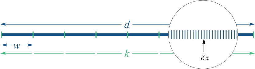
Figure 2: Periodic one dimensional lattice with $d$ lattice sites in total, $w$ lattice sites in each coarse-graining interval, and $k=d/w$ intervals. The lattice unit of length is $\delta x$.

In principle, realistic finite resolution measurements should be modeled as unsharp POVMs (Busch et al., 1996; Peres, 2006), where each POVM element is centered around a certain outcome value but has a non-zero probability (usually Gaussian) to respond to the adjacent values as well. In order to simplify the calculations we will consider an idealized version of that in the form of coarse-grained projective measurements. That is, each POVM element is a projection on a subspace associated with a range of values such that an outcome associate with each projection does not distinguish between any of the values in the range.

We introduce the integer parameters $w_{x}$, $w_{p}$ to specify the widths of the coarse-graining intervals for the corresponding observables (larger $w$ means lower resolution). The variable $k=d/w$ specifies the number of coarse-graining intervals which we will also assume to be an integer. See Fig. 2 for a diagrammatic summary of the relevant lengths.

The coarse-grained position and momentum observables are constructed from the spectral projections

$$\Pi_{X;\nu} =\sum_{n=\nu w_{x}}^{\nu w_{x}+w_{x}-1}\left|X;n\right\rangle\left\langle X;n\right|$$

$$\Pi_{P;\mu} =\sum_{m=\mu w_{p}}^{\mu w_{p}+w_{p}-1}\left|P;m\right\rangle\left\langle P;m\right|$$

associated with the eigenvalues of coarse-grained position $\nu=0,...,k_{x}-1$ and momentum $\mu=0,...,k_{p}-1$. The coarse-grained observables are then given by

$$X_{cg}=\sum_{\nu=0}^{k_{x}-1}\nu\,\Pi_{X;\nu}\,\,\,\,\,\,\,\,\,\,\,\,\,\,\,P_{cg}=\sum_{\mu=0}^{k_{p}-1}\mu\,\Pi_{P;\mu}.$$

In the following, we only compute the probabilities of outcomes so $P_{cg}$ and $X_{cg}$ are only shown here for the sake of completeness; the spectral projections $\Pi_{X;\nu}$ and $\Pi_{P;\mu}$ is all we need.

Let us now calculate the probability of getting the outcomes $\nu,\mu,\nu$ in an instantaneous sequence of position-momentum-position measurements on the initial state $\rho$. If $\rho^{\left(\nu\right)}$, $\rho^{\left(\nu\mu\right)}$ are the intermediate post-measurement states in this sequence then we can express this probability as

$$\boldsymbol{p}_{xpx}\left(\nu,\mu,\nu|\rho\right) =tr\left[\Pi_{X;\nu}\rho\right]tr\left[\Pi_{P;\mu}\rho^{\left(\nu\right)}\right]tr\left[\Pi_{X;\nu}\rho^{\left(\nu\mu\right)}\right]$$

$$=tr\left[\left(\Pi_{X;\nu}\Pi_{P;\mu}\Pi_{X;\nu}\right)^{2}\rho\right]$$ (3)

where the last line follows using explicit expressions for $\rho^{\left(\nu\right)}$ and $\rho^{\left(\nu\mu\right)}$. Then, the probability that both position outcomes agree, regardless of the outcomes, is

$$\boldsymbol{p}_{\textrm{agree}}\left(\rho\right) =\sum_{v=0}^{k_{x}-1}\sum_{\mu=0}^{k_{p}-1}\boldsymbol{p}_{xpx}\left(\nu,\mu,\nu|\rho\right)$$

$$=tr\left[\sum_{v=0}^{k_{x}-1}\sum_{\mu=0}^{k_{p}-1}\left(\Pi_{X;\nu}\Pi_{P;\mu}\Pi_{X;\nu}\right)^{2}\rho\right].$$ (4)

From Eq. (4) we identify the observable

$$\Lambda_{\textrm{agree}}=\sum_{\nu=0}^{k_{x}-1}\sum_{\mu=0}^{k_{p}-1}\left(\Pi_{X;\nu}\Pi_{P;\mu}\Pi_{X;\nu}\right)^{2}$$

whose expectation values are the probabilities $\boldsymbol{p}_{\textrm{agree}}\left(\rho\right)=tr\left(\Lambda_{\textrm{agree}}\rho\right)$.

Since $\boldsymbol{p}_{\textrm{agree}}\left(\rho\right)$ is linear in $\rho$, the average $\left\langle\boldsymbol{p}_{\textrm{agree}}\right\rangle$ is given by $\boldsymbol{p}_{\textrm{agree}}\left(\left\langle\rho\right\rangle\right)$ where $\left\langle\rho\right\rangle=\frac{1}{d}I$ is the average state. We can then calculate

$$\left\langle\boldsymbol{p}_{\textrm{agree}}\right\rangle =\boldsymbol{p}_{\textrm{agree}}\left(\frac{1}{d}I\right)=\frac{1}{d}tr\left[\Lambda_{\textrm{agree}}\right]$$

$$=\frac{w_{x}}{d}+\frac{2}{w_{x}w_{p}d}\sum_{n=1}^{w_{p}-1}\left(w_{p}-n\right)\frac{\sin^{2}\left(\frac{\pi nw_{x}}{d}\right)}{\sin^{2}\left(\frac{\pi n}{d}\right)}$$ (5)

(see Appendix B for the details of this calculation).

(a)

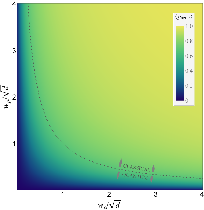
(b)

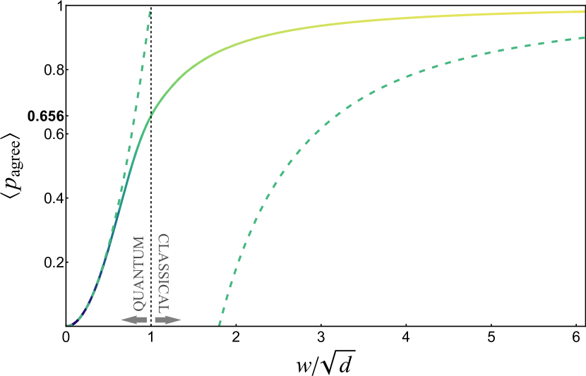
Figure 3: (a) The plot of the average probability $\left\langle\boldsymbol{p}_{\textrm{agree}}\right\rangle$ that an instantaneous succession of position-momentum-position measurements will agree on both outcomes of position as a function of the resolution parameters $w_{x}$, $w_{p}$ on a lattice of length $d$. The dotted curve $w_{x}w_{p}=d$ is the boundary that outlines the intermediate scale with respect to which we distinguish the quantum and classical regimes. (b) The plot of $\left\langle\boldsymbol{p}_{\textrm{agree}}\right\rangle$ (solid) on the diagonal $w=w_{x}=w_{p}$ with the upper and lower bounds (dashed) from Eqs. (6) and (7).

The plot of $\left\langle\boldsymbol{p}_{\textrm{agree}}\right\rangle$ as a function of $w_{x}$, $w_{p}$ is shown in Fig. 3(a) which makes it clear that $\left\langle\boldsymbol{p}_{\textrm{agree}}\right\rangle$ is symmetric under the exchange of $w_{x}$ with $w_{p}$. The plot of $\left\langle\boldsymbol{p}_{\textrm{agree}}\right\rangle$ along the diagonal $w=w_{x}=w_{p}$ is shown in Fig. 3(b) together with the upper and lower bounds

$$\left\langle\boldsymbol{p}_{\textrm{agree}}\right\rangle\leq w^{2}/d w<\sqrt{d}$$ (6)

$$\left\langle\boldsymbol{p}_{\textrm{agree}}\right\rangle\geq 1-\frac{2}{\pi^{2}}\frac{\ln\left(w^{2}/d\right)+3\pi^{2}/2}{w^{2}/d} w>\sqrt{d}$$ (7)

(see Appendix D for the derivation). Note that $\sqrt{d}$ distinguishes the two separate domains where these bounds are valid.

The upper bound (6) tells us that when $w<\sqrt{d}$, the value of $\left\langle\boldsymbol{p}_{\textrm{agree}}\right\rangle$ falls to $0$ at least as fast as $\sim w^{2}$. The lower bound (7) tells us that when $w>\sqrt{d}$, the value of $\left\langle\boldsymbol{p}_{\textrm{agree}}\right\rangle$ climbs to $1$ at least as fast as $\sim 1-\frac{\ln w^{2}}{w^{2}}$. The fact that the domains of these bounds are separated by $\sqrt{d}$, implies that there is an inflection in $\left\langle\boldsymbol{p}_{\textrm{agree}}\right\rangle$ somewhere around $w=\sqrt{d}$ along the diagonal $w=w_{x}=w_{p}$. That is, $\sqrt{d}$ is an intermediate scale where neither bound applies so it can serve as a reference point with respect to which we distinguish the quantum and classical regimes.

The above observation can be extended to the entire plane of $w_{x}$, $w_{p}$, where the curve $w_{x}w_{p}=d$ generalizes the point $w=\sqrt{d}$. According to the plot in Fig. 3(a), as we get farther from the curve $w_{x}w_{p}=d$, we get deeper into one of the regimes, and an inflection in $\left\langle\boldsymbol{p}_{\textrm{agree}}\right\rangle$ occurs somewhere near the curve. It can be shown (see Appendix C) that the intermediate value $\left\langle\boldsymbol{p}_{\textrm{agree}}\right\rangle\approx 0.656$ holds almost everywhere on this curve, except the far ends where it climbs to $1$.

There is nothing special about the value $0.656$, however, the significance of the curve $w_{x}w_{p}=d$ is that it outlines the intermediate scale in phase space with respect to which we can distinguish the quantum regime from the classical. That is, the curve $w_{x}w_{p}=d$ sets a reference scale so we can say that

$$\begin{cases}\left\langle\boldsymbol{p}_{\textrm{agree}}\right\rangle\approx 1&w_{x}w_{p}\gg d\\ \left\langle\boldsymbol{p}_{\textrm{agree}}\right\rangle\approx 0&w_{x}w_{p}\ll d.\end{cases}$$

We can of course say the same about $w_{x}w_{p}=cd$ for some $c\neq 1$; the important fact is that the constraint $cd$ depends linearly on $d$. We will see below that for $c=1$ this constraint corresponds exactly to the Planck constant.

III The continuum limit and the implications of minimal length

III.1 Perturbations of $\left\langle\boldsymbol{p}_{\textrm{agree}}\right\rangle$

We will now introduce proper units. The total length of the lattice in proper units is $L=\delta xd$, where $\delta x$ is the smallest unit of length associated with one lattice spacing. The smallest unit of inverse length, or a wavenumber, is then $1/L$. With the de Broglie relation $p=2\pi\hbar/\lambda$, we can convert wavenumbers $1/\lambda$ to momenta, so the smallest unit of momentum is $\delta p=2\pi\hbar/L$. The coarse-graining intervals $w_{x}$ and $w_{p}$ become $\Delta x=\delta xw_{x}$ and $\Delta p=\delta pw_{p}$ when expressed in proper units.

The continuum limit can be achieved by taking $\delta x\rightarrow 0$ and $d\rightarrow\infty$ while keeping $L$ constant. The coarse-graining interval of position $\Delta x=\delta xw_{x}$ is kept constant as well by fixing the total number of intervals $k_{x}=d/w_{x}$ while $w_{x}\rightarrow\infty$. Unlike $\delta x$, $\delta p=2\pi\hbar/L$ does not vanish in the continuum limit (the momentum of a particle in a box remains quantized) so the coarse-graining intervals of momentum $\Delta p=\delta pw_{p}$ are unaffected and $w_{p}$ remains a finite integer.

We may now ask what happens to $\left\langle\boldsymbol{p}_{\textrm{agree}}\right\rangle$ as we take the continuum limit. Since $w_{x}/d=\Delta x/L$, the expression in Eq. (5) can be re-expressed using the proper units of length as

$$\left\langle\boldsymbol{p}_{\textrm{agree}}\right\rangle=\frac{\Delta x}{L}+\frac{L}{\Delta x}\frac{2}{w_{p}}\sum_{n=1}^{w_{p}-1}\left(w_{p}-n\right)\frac{\sin^{2}\left(\frac{\pi n\Delta x}{L}\right)}{\left[d\sin\left(\frac{\pi n}{d}\right)\right]^{2}}.$$ (8)

We did not have to use the proper units of momentum since

$$w_{p}=\frac{\Delta p}{\delta p}=\frac{\Delta p}{2\pi\hbar}L,$$

which is a legitimate quantity even in the continuum limit (provided that $L$ is finite).

The only evidence for the lattice structure that remains in Eq. (8) is the $d$-dependence of the factors

$$\left[d\sin\left(\frac{\pi n}{d}\right)\right]^{-2}=\frac{1}{\pi^{2}n^{2}}+\frac{1}{3d^{2}}+O\left(\frac{1}{d^{3}}\right).$$

In the continuum limit they reduce to $1/\pi^{2}n^{2}$, but when the minimal length $\delta x=L/d$ is above $0$, these factors are perturbed with the leading order contribution of $1/3d^{2}$.

The leading order perturbation term of $\left\langle\boldsymbol{p}_{\textrm{agree}}\right\rangle$ is therefore

$$\left\langle\boldsymbol{p}_{\textrm{agree}}\right\rangle_{\textrm{pert.}} =\frac{L}{\Delta x}\frac{2}{w_{p}}\sum_{n=1}^{w_{p}-1}\left(w_{p}-n\right)\frac{\sin^{2}\left(\frac{\pi n\Delta x}{L}\right)}{3d^{2}}$$

$$=\frac{2}{3w_{x}w_{p}d}\sum_{n=1}^{w_{p}-1}\left(w_{p}-n\right)\sin^{2}\left(\frac{\pi nw_{x}}{d}\right)$$ (9)

and we reverted to the lattice units in the last step. In Fig. 4(a) we have plotted Eq. (9) for $d=10^{4}$. As we can see from the plot, the lattice perturbation gets stronger as $w_{x}$ decreases and $w_{p}$ increases, and the perturbation spikes in the regime where $w_{x}<\sqrt{d}$ and $w_{p}>\sqrt{d}$.

Focusing on this regime, we can assume that $w_{p}\gg 1$ (since $\sqrt{d}\gg 1$) and approximate the sum with an integral. That is,

$$\left\langle\boldsymbol{p}_{\textrm{agree}}\right\rangle_{\textrm{pert.}} =\frac{2w_{p}}{3w_{x}d}\sum_{n=1}^{w_{p}-1}\frac{1}{w_{p}}\left(1-\frac{n}{w_{p}}\right)\sin^{2}\left(\frac{\pi nw_{x}w_{p}}{w_{p}d}\right)$$

$$\approx\frac{2}{3}\frac{w_{p}}{w_{x}d}\int_{0}^{1}d\alpha\left(1-\alpha\right)\sin^{2}\left(\pi\alpha\frac{w_{x}w_{p}}{d}\right)$$

$$=\frac{2}{3}\frac{w_{p}}{w_{x}d}\left[\frac{1}{4}+\frac{\cos(2\pi w_{x}w_{p}/d)-1}{8\pi^{2}\left(w_{x}w_{p}/d\right)^{2}}\right].$$ (10)

See Fig. 4(b) for the plot of Eq. (10). By re-introducing proper units and rearranging we get

$$\left\langle\boldsymbol{p}_{\textrm{agree}}\right\rangle_{\textrm{pert.}}\approx\frac{1}{6\pi}\left(\frac{\delta x}{\Delta x}\right)^{2}\left[\frac{1}{2}\frac{\Delta x\Delta p}{\hbar}+\frac{\cos(\Delta x\Delta p/\hbar)-1}{\Delta x\Delta p/\hbar}\right].$$

In particular, on the curve $\Delta x\Delta p=2\pi\hbar$ we have $\left\langle\boldsymbol{p}_{\textrm{agree}}\right\rangle_{\textrm{pert.}}\approx\frac{1}{6}\left(\delta x/\Delta x\right)^{2}$ so the perturbation keeps growing as we ascend on this curve.

Since $\left\langle\boldsymbol{p}_{\textrm{agree}}\right\rangle$ is an operationally defined quantity, it in principle can be measured. The perturbation term $\left\langle\boldsymbol{p}_{\textrm{agree}}\right\rangle_{\textrm{pert.}}$ can therefore be leveraged as a signal of the discontinuity of space in experimental approaches. That is, given the continuum probabilities

$$\left\langle\boldsymbol{p}_{\textrm{agree}}\right\rangle_{\textrm{cont.}}=\frac{\Delta x}{L}+\frac{L}{\Delta x}\frac{2}{w_{p}}\sum_{n=1}^{w_{p}-1}\left(w_{p}-n\right)\frac{\sin^{2}\left(\frac{\pi n\Delta x}{L}\right)}{\pi^{2}n^{2}}$$

we expect to find that

$$\left\langle\boldsymbol{p}_{\textrm{agree}}\right\rangle=\left\langle\boldsymbol{p}_{\textrm{agree}}\right\rangle_{\textrm{cont.}}+\left\langle\boldsymbol{p}_{\textrm{agree}}\right\rangle_{\textrm{pert.}}+O\left(\frac{1}{d^{3}}\right)$$

so by measuring the deviation of $\left\langle\boldsymbol{p}_{\textrm{agree}}\right\rangle$ from the value of $\left\langle\boldsymbol{p}_{\textrm{agree}}\right\rangle_{\textrm{cont.}}$ as defined above, we can detect the discontinuity of space.

For realistic values of $d$ the signal of $\left\langle\boldsymbol{p}_{\textrm{agree}}\right\rangle_{\textrm{pert.}}$ is of course extremely weak. However, the “humps” of $\left\langle\boldsymbol{p}_{\textrm{agree}}\right\rangle_{\textrm{pert.}}$ start to appear on the intermediate scales of $\Delta x<\delta x\sqrt{d}$ and $\Delta p>\delta p\sqrt{d}$ (see Fig. 4(b)), so we do not have to go to the extremes of minimal length or maximal momentum to look for them.

(a)

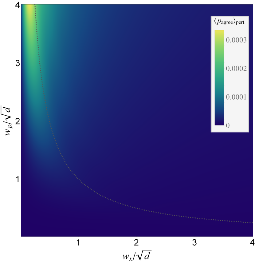
(b)

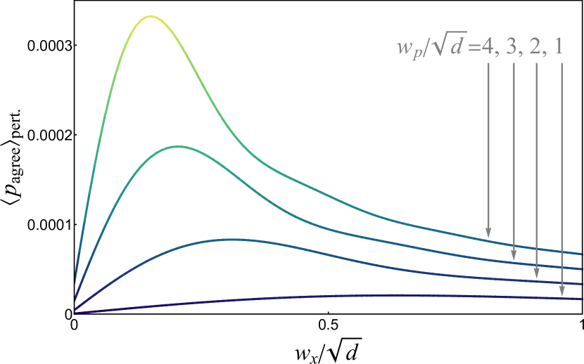
Figure 4: (a) The plot of the perturbation of $\left\langle\boldsymbol{p}_{\textrm{agree}}\right\rangle$ on a lattice of length $d=10^{4}$ as given by Eq. (9) (the dotted curve is $w_{x}w_{p}=d$). (b) The profile of the perturbation as given by Eq. (10) for $w_{p}/\sqrt{d}=1,2,3,4$ and $d=10^{4}$.

III.2 Factorizing the Planck constant

With the introduction of proper units we observe that the smallest unit of phase space area on a lattice is $\delta x\delta p=2\pi\hbar/d$. Therefore, the curve $w_{x}w_{p}=d$ that outlines the intermediate scale in phase space becomes

$$\Delta x\Delta p=\delta x\delta p\,w_{x}w_{p}=\delta x\delta p\,d=2\pi\hbar.$$ (11)

Thus, we have recovered Heisenberg’s original argument that the Planck constant sets the scale in phase space where the mutual disturbance effects become significant. Note that Eq. (11) is related to what is known as the error-disturbance uncertainty relations (not to be confused with the preparation uncertainty relations). We thus see that in the unitless lattice setting (where $\delta x\equiv 1$ and $\delta p\equiv 1$) the constant $d$ is the unitless “Planck constant”.

In the continuous phase space, the uncertainty principle is only associated with the constant $2\pi\hbar$, which does not admit a preferred factorization into position and momentum. On the lattice, however, the same constant is given by $\delta x\delta pd$, which can be factorized as $\delta x\sqrt{d}$ and $\delta p\sqrt{d}$. This factorization is not arbitrary and the significance of the scales $\delta x\sqrt{d}$ and $\delta p\sqrt{d}$ is supported by the analysis of $\left\langle\boldsymbol{p}_{\textrm{agree}}\right\rangle$. In particular, we saw that the perturbation $\left\langle\boldsymbol{p}_{\textrm{agree}}\right\rangle_{\textrm{pert.}}$ due to the discontinuity of the lattice spikes in the regime where $\Delta x<\delta x\sqrt{d}$ and $\Delta p>\delta p\sqrt{d}$.

The significance of the scale $\sqrt{d}$ on a lattice can also be observed from $\left\langle\boldsymbol{p}_{\textrm{agree}}\right\rangle$ directly. In Fig. 3(a) we can see that when the localization in position $w_{x}$ crosses $\sqrt{d}$ from above, the localization in momentum $w_{p}$ has to diverge faster than it converges in $w_{x}$ in order to stay in the classical regime. In contrast, as long as both $w_{x},w_{p}\gg\sqrt{d}$, the classical regime is insensitive to the variations in these variables and there is no need to compensate the increase in localization for one variable with the decrease in localization for the other.

This observation is directly analogous to the analysis of Kofler and Brukner in (Kofler and Brukner, 2007) (similar question have been considered in (Poulin, 2005) and (Peres, 2006)) where they have demonstrated that for a spin-$j$ system, incompatible spin components can simultaneously be determined if the resolution of measurements is coarse compared to $\sqrt{j}$. Our analysis show that the same conclusion applies to position and momentum on a lattice, where both variables can simultaneously be determined if the resolution of measurements is coarse compared to $\sqrt{d}$.

The uncertainty principle on a lattice can therefore primarily be associated with the unitless scale $\sqrt{d}$, which identifies the intermediate scales $\delta x\sqrt{d}$ and $\delta p\sqrt{d}$ for position and momentum. The intermediate scale in phase space is in turn given by

$$\left(\delta x\sqrt{d}\right)\left(\delta p\sqrt{d}\right)=\delta x\delta p\,d=2\pi\hbar.$$

The intermediate length scale $\delta x\sqrt{d}$ can be identified as the scale around which increases in localization in position result in equal decreases in localization in momentum, and vice versa. Of course, this definition is only meaningful on a lattice because it requires the fundamental units $\delta x$ and $\delta p$ in terms of which we can compare the changes in localization for both variables. Nevertheless, we conclude that on a lattice, in addition to the minimal length $\delta x$ and the maximal length $L$, the uncertainty principle singles out another significant length

$$l_{u}=\delta x\sqrt{d}.$$

The length $l_{u}$ is directly related to the minimal length $\delta x$ via $L=\delta xd$ as $l_{u}=\sqrt{\delta x\,L}$ or $\delta x=l_{u}^{2}/L$. The length $l_{u}$ is therefore the geometric mean of the minimal length $\delta x$ and the maximal length $L$. It can also be framed as the length for which there are as many intervals $l_{u}$ in $L$ as there are $\delta x$ in $l_{u}$. In the continuum limit, where the minimal length $\delta x$ vanishes, the length $l_{u}=\sqrt{\delta x\,L}$ must also vanish. Therefore, if we can establish that $l_{u}>0$ then it follows that $\delta x>0$.

We saw that the perturbations of $\left\langle\boldsymbol{p}_{\textrm{agree}}\right\rangle$ spike in the regime where $\Delta x<l_{u}$, but it is not clear at this point what realistically observable effects can be associated with the length $l_{u}$. If such effects can be identified, however, then the discontinuity of space can be probed at scales that are many orders of magnitude greater than the Planck length. For instance, for $L\sim 1\,\textrm{m}$ of the order of a macroscopic box and $\delta x\sim 10^{-35}\,\textrm{m}$ of the order of Planck length, we have $l_{u}\sim 10^{-17.5}\,\textrm{m}$ which is much closer to the scale of experiments.

IV Conclusion

In the present work we have studied the effects of the uncertainty principle on a finite-dimensional periodic lattice, and their dependence on minimal length. Instead of modifying the canonical commutation relations, we have operationally quantified the mutual disturbance effects with the average probability $\left\langle\boldsymbol{p}_{\textrm{agree}}\right\rangle$, and compared it to the continuum limit.

The analysis of $\left\langle\boldsymbol{p}_{\textrm{agree}}\right\rangle$ indicated that $\sqrt{d}$ is a significant scale on a lattice that separates the classical regime of joint measurability, from the quantum regime where mutual disturbance effect are important. In the units of length, the scale $\sqrt{d}$ corresponds to the geometric mean $l_{u}=\sqrt{\delta xL}$ of the minimal length $\delta x$ and the maximal length $L$, and in phase space it corresponds to the Planck constant. This result is consistent with the conclusion of Kofler and Brukner (Kofler and Brukner, 2007) for spin-$j$ systems where incompatible observables can simultaneously be determined if the resolution of measurements is coarse compared to $\sqrt{j}$.

We have also analyzed the perturbations of $\left\langle\boldsymbol{p}_{\textrm{agree}}\right\rangle$ due to the non-vanishing minimal length $\delta x$ on a lattice. As a result, we saw that the perturbations become pronounced in the regime where the resolution in position falls below the scale of $l_{u}$, and the resolution in momentum rises above the scale of $\delta p\sqrt{d}$.

This is a preliminary result and we make no attempt to translate it into experimental predictions. For a more concrete experimental proposal it will be necessary to repeat the analysis of $\boldsymbol{p}_{\textrm{agree}}$ with the experimentally accessible ensemble of states $\rho$. Furthermore, depending on the experimental implementation, it will be necessary to use the non-idealized coarse-grained measurements and (possibly) account for the time evolution inbetween or during the measurements. Nonetheless, this result indicates that in principle it is possible to detect the discontinuity of the underlying space on the intermediate scales associated with $\sqrt{d}$.

Appendix A General definitions and identities

As described above, we are dealing with the $d$-dimensional Hilbert space of a particle on a periodic lattice with the position and momentum basis related via the discrete Fourier transform $F$. The translation operators $T_{X}$, $T_{P}$ in position and momentum can be defined by their action on the basis (Vourdas, 2004) as follows

$$T_{X}\left|X;n\right\rangle =\left|X;n+1\right\rangle T_{X}^{\dagger}\left|X;n\right\rangle=\left|X;n-1\right\rangle$$

$$T_{P}\left|P;m\right\rangle =\left|P;m+1\right\rangle T_{P}^{\dagger}\left|P;m\right\rangle=\left|P;m-1\right\rangle$$

where $\pm 1$ are $\mathsf{mod}\,d$. By expanding the position basis in momentum basis and vice versa and using the definitions, it is straight forward to verify that

$$T_{P}\left|X;n\right\rangle =e^{i2\pi n/d}\left|X;n\right\rangle T_{P}^{\dagger}\left|X;n\right\rangle=e^{-i2\pi n/d}\left|X;n\right\rangle$$

$$T_{X}\left|P;m\right\rangle =e^{-i2\pi m/d}\left|P;m\right\rangle T_{X}^{\dagger}\left|P;m\right\rangle=e^{i2\pi m/d}\left|P;m\right\rangle.$$

Therefore, $T_{P}$ commutes with $\left|X;n\right\rangle\left\langle X;n\right|$ and so does $T_{X}$ with $\left|P;m\right\rangle\left\langle P;m\right|$. This also means that $T_{P}$ commutes with $\Pi_{X;\nu}$ and $T_{X}$ commutes with $\Pi_{P;\mu}$.

Using the translation operators we can express the coarse-grained position and momentum projections as

$$\Pi_{X;\nu} =T_{X}^{\nu w_{x}}\Pi_{X;0}T_{X}^{\nu w_{x}\dagger} \Pi_{P;\mu}=T_{P}^{\mu w_{p}}\Pi_{P;0}T_{P}^{\mu w_{p}\dagger}.$$

Then, using the commutativity of projections with translations we get the identity

$$\Pi_{X;\nu}\Pi_{P;\mu}\Pi_{X;\nu}=T_{P}^{\mu w_{p}}\left(\Pi_{X;\nu}\Pi_{P;0}\Pi_{X;\nu}\right)T_{P}^{\mu w_{p}\dagger}=T_{P}^{\mu w_{p}}T_{X}^{\nu w_{x}}\left(\Pi_{X;0}\Pi_{P;0}\Pi_{X;0}\right)T_{X}^{\nu w_{x}\dagger}T_{P}^{\mu w_{p}\dagger}.$$ (12)

Focusing on the $\nu=\mu=0$ case we can express

$$\Pi_{X;0}\Pi_{P;0}\Pi_{X;0}=\sum_{m=0}^{w_{p}-1}\Pi_{X;0}\left|P;m\right\rangle\left\langle P;m\right|\Pi_{X;0}=\frac{1}{k_{x}}\sum_{m=0}^{w_{p}-1}\left|P_{0};m\right\rangle\left\langle P_{0};m\right|.$$ (13)

Thus, we define the truncated momentum states which are given by the normalized support of the $m$’th momentum state on the $\nu$’th position interval:

$$\left|P_{\nu};m\right\rangle :=\sqrt{k_{x}}\,\Pi_{X;\nu}\left|P;m\right\rangle=\frac{1}{\sqrt{w_{x}}}\sum_{n=\nu w_{x}}^{\nu w_{x}+w_{x}-1}e^{i2\pi mn/d}\left|X;n\right\rangle.$$ (14)

In general, these states are not orthogonal and their overlap is given by

$$\left.\left\langle P_{\nu^{\prime}};m^{\prime}\right.\,\right|\left.P_{\nu};m\right\rangle =\delta_{\nu^{\prime},\nu}k_{x}\left\langle P;m^{\prime}\right|\Pi_{X;\nu}\left|P;m\right\rangle=\delta_{\nu^{\prime},\nu}\frac{k_{x}}{d}\sum_{n=\nu w_{x}}^{\nu w_{x}+w_{x}-1}e^{i2\pi\left(m-m^{\prime}\right)n/d}.$$

It will be convenient to identify sums such as the one above, by defining the function

$$\varDelta_{q}\left(x\right):=\frac{1}{q}\sum_{n=0}^{q-1}e^{i2\pi xn/q}=\frac{e^{i\pi\left(x-x/q\right)}}{q}\frac{\sin\left(\pi x\right)}{\sin\left(\pi x/q\right)}$$ (15)

over real $x$ and integer $q\geq 1$. Note that $\varDelta_{q}\left(0\right)=1$. Then, for $\nu^{\prime}=\nu=0$ the overlap of truncated momentum states can be expressed as

$$\left.\left\langle P_{0};m^{\prime}\right.\,\right|\left.P_{0};m\right\rangle =\varDelta_{w_{x}}\left(\frac{m-m^{\prime}}{k_{x}}\right).$$ (16)

Appendix B Calculation of Eq. (5)

Given the operator

$$\Lambda_{\textrm{agree}}=\sum_{\nu=0}^{k_{x}-1}\sum_{\mu=0}^{k_{p}-1}\left(\Pi_{X;\nu}\Pi_{P;\mu}\Pi_{X;\nu}\right)^{2}$$

we are interested in the quantity $\left\langle\boldsymbol{p}_{\textrm{agree}}\right\rangle=\frac{1}{d}tr\left[\Lambda_{\textrm{agree}}\right]$. Using the identity (12) we can simplify the problem:

$$\left\langle\boldsymbol{p}_{\textrm{agree}}\right\rangle=\frac{1}{d}tr\left[\sum_{\nu=0}^{k_{x}-1}\sum_{\mu=0}^{k_{p}-1}\left(\Pi_{X;\nu}\Pi_{P;\mu}\Pi_{X;\nu}\right)^{2}\right]=\frac{k_{x}k_{p}}{d}tr\left[\left(\Pi_{X;0}\Pi_{P;0}\Pi_{X;0}\right)^{2}\right].$$ (17)

Using (13) and (16) we can further simplify

$$\left\langle\boldsymbol{p}_{\textrm{agree}}\right\rangle=\frac{1}{d}\frac{k_{p}}{k_{x}}\sum_{m,m^{\prime}=0}^{w_{p}-1}\left|\left.\left\langle P_{0};m^{\prime}\right.\,\right|\left.P_{0};m\right\rangle\right|^{2}=\frac{1}{d}\frac{k_{p}}{k_{x}}\sum_{m,m^{\prime}=0}^{w_{p}-1}\left|\varDelta_{w_{x}}\left(\frac{m-m^{\prime}}{k_{x}}\right)\right|^{2}.$$

Since the summand depends only on the difference $n=m-m^{\prime}$, we can re-express the sum in terms of the single variable $n$

$$\left\langle\boldsymbol{p}_{\textrm{agree}}\right\rangle=\frac{1}{d}\frac{k_{p}}{k_{x}}\sum_{n=-w_{p}+1}^{w_{p}-1}\left(w_{p}-\left|n\right|\right)\left|\varDelta_{w_{x}}\left(\frac{n}{k_{x}}\right)\right|^{2}.$$

Since the summed function is symmetric $\left|\varDelta_{w_{x}}\left(x\right)\right|^{2}=\left|\varDelta_{w_{x}}\left(-x\right)\right|^{2}$, we have

$$\left\langle\boldsymbol{p}_{\textrm{agree}}\right\rangle=\frac{1}{d}\frac{k_{p}}{k_{x}}\left[w_{p}\left|\varDelta_{w_{x}}\left(0\right)\right|^{2}+2\sum_{n=1}^{w_{p}-1}\left(w_{p}-n\right)\left|\varDelta_{w_{x}}\left(\frac{n}{k_{x}}\right)\right|^{2}\right].$$

Substituting the definition (15) of $\varDelta_{w_{x}}$ and recalling that $\varDelta_{w_{x}}\left(0\right)=1$ and that $k_{x}=d/w_{x}$ and $k_{p}=d/w_{p}$, we get the result

$$\left\langle\boldsymbol{p}_{\textrm{agree}}\right\rangle =\frac{1}{d}\frac{w_{x}}{w_{p}}\left[w_{p}+2\sum_{n=1}^{w_{p}-1}\left(w_{p}-n\right)\frac{1}{w_{x}^{2}}\frac{\sin^{2}\left(\frac{\pi nw_{x}}{d}\right)}{\sin^{2}\left(\frac{\pi n}{d}\right)}\right]$$

$$=\frac{w_{x}}{d}+\frac{2}{w_{x}w_{p}d}\sum_{n=1}^{w_{p}-1}\left(w_{p}-n\right)\frac{\sin^{2}\left(\frac{\pi nw_{x}}{d}\right)}{\sin^{2}\left(\frac{\pi n}{d}\right)}.$$ (18)

The apparent asymmetry under the exchange of $w_{x}$ with $w_{p}$ in the result (18), traces back to the apparent asymmetry under the exchange between $\Pi_{X;0}$ and $\Pi_{P;0}$ in the expression (17). These asymmetries are only apparent because

$$tr\left[\left(\Pi_{X;0}\Pi_{P;0}\Pi_{X;0}\right)^{2}\right]=tr\left[\Pi_{X;0}\Pi_{P;0}\Pi_{X;0}\Pi_{P;0}\right]=tr\left[\left(\Pi_{P;0}\Pi_{X;0}\Pi_{P;0}\right)^{2}\right],$$

so if we were to change the order in expression (17) to $tr\left[\left(\Pi_{P;0}\Pi_{X;0}\Pi_{P;0}\right)^{2}\right]$, we would end up with

$$\left\langle\boldsymbol{p}_{\textrm{agree}}\right\rangle=\frac{w_{p}}{d}+\frac{2}{w_{x}w_{p}d}\sum_{n=1}^{w_{x}-1}\left(w_{x}-n\right)\frac{\sin^{2}\left(\frac{\pi nw_{p}}{d}\right)}{\sin^{2}\left(\frac{\pi n}{d}\right)}.$$

The form (18) is better suited for the continuum limit where $w_{p}$ remains finite while $w_{x}$ is not (but $\frac{w_{x}}{d}$ is).

Appendix C The value of $\left\langle\boldsymbol{p}_{\textrm{agree}}\right\rangle$ on the curve $w_{x}w_{p}=d$

When $w_{x}w_{p}=d$ we can simplify

$$\left\langle\boldsymbol{p}_{\textrm{agree}}\right\rangle=\frac{1}{w_{p}}+\frac{2}{d^{2}}\sum_{n=1}^{w_{p}-1}\left(w_{p}-n\right)\frac{\sin^{2}\left(\frac{\pi n}{w_{p}}\right)}{\sin^{2}\left(\frac{\pi n}{d}\right)}.$$ (19)

First, let us consider the intermediate range of values $1\ll w_{p}\ll d$, which includes $w_{p}=\sqrt{d}$ provided that $1\ll d$. Since $n<w_{p}\ll d$ we can approximate $\sin^{-2}\left(\frac{\pi n}{d}\right)\approx\left(\frac{\pi n}{d}\right)^{-2}$ and so

$$\left\langle\boldsymbol{p}_{\textrm{agree}}\right\rangle\approx\frac{1}{w_{p}}+\frac{2}{\pi^{2}}\sum_{n=1}^{w_{p}-1}\left(w_{p}-n\right)\frac{\sin^{2}\left(\frac{\pi n}{w_{p}}\right)}{n^{2}}.$$ (20)

Since $1\ll w_{p}$, we can approximate the sum with an integral by introducing the variable $\alpha=\frac{n}{w_{p}}\in\left[0,1\right]$ and $d\alpha=\frac{1}{w_{p}}$, such that

$$\left\langle\boldsymbol{p}_{\textrm{agree}}\right\rangle \approx\frac{1}{w_{p}}+\frac{2}{\pi^{2}}\sum_{n=1}^{w_{p}-1}\frac{1}{w_{p}}\left(1-\frac{n}{w_{p}}\right)\frac{\sin^{2}\left(\pi\frac{n}{w_{p}}\right)}{n^{2}/w_{p}^{2}}$$

$$\approx d\alpha+\frac{2}{\pi^{2}}\int_{0}^{1}d\alpha\left(1-\alpha\right)\frac{\sin^{2}\left(\pi\alpha\right)}{\alpha^{2}}\approx 0.656.$$

Thus, $\left\langle\boldsymbol{p}_{\textrm{agree}}\right\rangle\approx 0.656$ for $1\ll w_{p}\ll d$ on the curve $w_{x}w_{p}=d$.

When the values of $w_{p}$ are close to $1$, we cannot assume that $1\ll w_{p}$ but $w_{p}\ll d$ still holds so we can still use the approximation (20). For $w_{p}=1$ the sum in (20) vanishes and we are left with $\left\langle\boldsymbol{p}_{\textrm{agree}}\right\rangle=1/w_{p}=1$ (we can also see that from Eq. (17) that is easy to evaluate for $w_{p}=1$, and $w_{x}=d$). Numerically evaluating Eq. (20) for the subsequent values of $w_{p}$ results in the following series (considering only $3$ significant figures)

$w_{p}$	1	2	3	4	…	15	16	…
$\left\langle\boldsymbol{p}_{\textrm{agree}}\right\rangle$	$1.00$	$0.703$	$0.675$	$0.667$	…	$0.657$	$0.656$	$0.656$

Thus, we can see that on one end of the curve $w_{x}w_{p}=d$, where the $w_{p}$’s are small, the function $\left\langle\boldsymbol{p}_{\textrm{agree}}\right\rangle$ reaches and stays on the value $0.656$ starting from $w_{p}\geq 16$.

Since $w_{x}$ and $w_{p}$ are interchangeable, we can re-express Eq. (20) as

$$\left\langle\boldsymbol{p}_{\textrm{agree}}\right\rangle\approx\frac{1}{w_{x}}+\frac{2}{\pi^{2}}\sum_{n=1}^{w_{x}-1}\left(w_{x}-n\right)\frac{\sin^{2}\left(\frac{\pi n}{w_{x}}\right)}{n^{2}}.$$

Then, on the other end of this curve, where the $w_{x}$’s are small, the function $\left\langle\boldsymbol{p}_{\textrm{agree}}\right\rangle$ reaches and stays on the value $0.656$ starting from $w_{x}\geq 16$. Therefore, $\left\langle\boldsymbol{p}_{\textrm{agree}}\right\rangle\approx 0.656$ almost everywhere on the curve $w_{x}w_{p}=d$, with the exception of the far ends where $w_{p}<16$ or $w_{x}<16$; there it climbs to $1$.

Appendix D Calculation of the bounds (6) and (7)

From here on, we will assume $w=w_{x}=w_{p}$ and $k=k_{x}=k_{p}$.

In order to calculate the bounds on $\left\langle\boldsymbol{p}_{\textrm{agree}}\right\rangle$ we will have to find a different way to express $\Pi_{X;0}\Pi_{P;0}\Pi_{X;0}$. Recalling Eq. (16) and the function (15) we now have

$$\left|\left.\left\langle P_{0};m^{\prime}\right.\,\right|\left.P_{0};m\right\rangle\right|=\left|\varDelta_{w}\left(\frac{m-m^{\prime}}{k}\right)\right|=\frac{\sin\left(\pi\frac{m-m^{\prime}}{k}\right)}{w\sin\left(\pi\frac{m-m^{\prime}}{d}\right)}.$$

Observe that the truncated momentum states are orthogonal when the difference $m-m^{\prime}$ is an integer number of $k$’s. That is, for any integers $c$, $c^{\prime}$ and $n$ the states $\left|P_{0};ck+n\right\rangle$ and $\left|P_{0};c^{\prime}k+n\right\rangle$ are orthogonal.

In Eq. (13) we have derived the form

$$\Pi_{X;0}\Pi_{P;0}\Pi_{X;0}=\frac{1}{k}\sum_{m=0}^{w-1}\left|P_{0};m\right\rangle\left\langle P_{0};m\right|$$ (21)

where $\left|P_{0};m\right\rangle\left\langle P_{0};m\right|$ are rank 1 projections. Since some of these projections are pairwise orthogonal, we can group them together and express $\Pi_{X;0}\Pi_{P;0}\Pi_{X;0}$ as a smaller sum of higher rank projections.

In order to do that, let us first assume that $\gamma=w/k$ is a non-zero integer (we will not need this assumption in general). Then the set of integers $\left\{m=0,...,w-1\right\}$ can be partitioned into $k$ subsets $\Omega_{n}=\left\{ck+n\,|\,c=0,...,\gamma-1\right\}$ with $n=0,...,k-1$. Thus, we can group up the orthogonal elements in the sum (21) as

$$\Pi_{X;0}\Pi_{P;0}\Pi_{X;0}=\frac{1}{k}\sum_{n=0}^{k-1}\sum_{m\in\Omega_{n}}\left|P_{0};m\right\rangle\left\langle P_{0};m\right|=\frac{1}{k}\sum_{n=0}^{k-1}\Pi^{\left(n\right)}$$

where we have introduced the rank $\gamma$ projections

$$\Pi^{\left(n\right)}=\sum_{m\in\Omega_{n}}\left|P_{0};m\right\rangle\left\langle P_{0};m\right|=\sum_{c=0}^{\gamma-1}\left|P_{0};ck+n\right\rangle\left\langle P_{0};ck+n\right|.$$

When $\gamma=w/k$ is not an integer, the accounting of indices is more involved. We have to introduce the integer part $g=\left\lfloor\gamma\right\rfloor$ and the remainder part $r=w-k\left\lfloor\gamma\right\rfloor$ of $\gamma$. As before, we partition the set $\left\{m=0,...,w-1\right\}$ into subsets

$$\Omega_{n}:=\begin{cases}\left\{ck+n\,|\,c=0,...,g\right\}&n<r\\ \left\{ck+n\,|\,c=0,...,g-1\right\}&n\geq r\end{cases}$$

but now they are not of equal size and the range of $n$ depends on whether $\gamma\geq 1$. When $\gamma\geq 1$ then $\left|\Omega_{n}\right|$ is $g+1$ for $n<r$ and $g$ for $n\geq r$. When $\gamma<1$ so $g=0$ and $r=w$, then $\left|\Omega_{n}\right|=1$ for $n<w$ but $\left|\Omega_{n}\right|=0$ for $n\geq w$ so we do not need to count $\Omega_{n}$ for $n\geq w$. Noting that the condition $\gamma\geq 1$ is equivalent to $\min\left(k,w\right)=k$ and the condition $\gamma<1$ is equivalent to $\min\left(k,w\right)=w$, we conclude that we only have to count $\Omega_{n}$ for $n<\min\left(k,w\right)$. Therefore, for the general $\gamma$ we have

$$\Pi_{X;0}\Pi_{P;0}\Pi_{X;0}=\frac{1}{k}\sum_{n=0}^{\min\left(k,w\right)-1}\sum_{m\in\Omega_{n}}\left|P_{0};m\right\rangle\left\langle P_{0};m\right|=\frac{1}{k}\sum_{n=0}^{\min\left(k,w\right)-1}\Pi^{\left(n\right)}$$ (22)

and the projections

$$\Pi^{\left(n\right)}=\sum_{m\in\Omega_{n}}\left|P_{0};m\right\rangle\left\langle P_{0};m\right|=\sum_{c=0}^{g_{n}-1}\left|P_{0};ck+n\right\rangle\left\langle P_{0};ck+n\right|$$

are now of the rank

$$g_{n}=\begin{cases}g+1&n<r\\ g&n\geq r.\end{cases}$$

Using the new form (22), we can re-express Eq. (17) as

$$\left\langle\boldsymbol{p}_{\textrm{agree}}\right\rangle=\frac{k^{2}}{d}tr\left[\left(\Pi_{X;0}\Pi_{P;0}\Pi_{X;0}\right)^{2}\right]=\frac{1}{d}\sum_{n,n^{\prime}=0}^{\min\left(k,w\right)-1}tr\left[\Pi^{\left(n\right)}\Pi^{\left(n^{\prime}\right)}\right].$$ (23)

The upper bound

The quantity $tr\left[\Pi^{\left(n\right)}\Pi^{\left(n^{\prime}\right)}\right]$ is the Hilbert-Schmidt inner product $\left\langle\Pi^{\left(n\right)},\Pi^{\left(n^{\prime}\right)}\right\rangle$ (also known as Frobenius inner product) of the operators $\Pi^{\left(n\right)}$ and $\Pi^{\left(n^{\prime}\right)}$. Therefore, it obeys the Cauchy–Schwarz inequality

$$\left|tr\left[\Pi^{\left(n\right)}\Pi^{\left(n^{\prime}\right)}\right]\right|^{2}=\left|\left\langle\Pi^{\left(n\right)},\Pi^{\left(n^{\prime}\right)}\right\rangle\right|^{2}\leq\left\langle\Pi^{\left(n\right)},\Pi^{\left(n\right)}\right\rangle\left\langle\Pi^{\left(n^{\prime}\right)},\Pi^{\left(n^{\prime}\right)}\right\rangle=tr\left[\Pi^{\left(n\right)}\right]tr\left[\Pi^{\left(n^{\prime}\right)}\right].$$

Since the value

$$tr\left[\Pi^{\left(n\right)}\Pi^{\left(n^{\prime}\right)}\right]=\sum_{m\in\Omega_{n}}\sum_{m^{\prime}\in\Omega_{n^{\prime}}}\left|\left.\left\langle P_{0};m\right.\,\right|\left.P_{0};m^{\prime}\right\rangle\right|^{2}$$

is clearly real and positive, we get

$$tr\left[\Pi^{\left(n\right)}\Pi^{\left(n^{\prime}\right)}\right]\leq\sqrt{tr\left[\Pi^{\left(n\right)}\right]tr\left[\Pi^{\left(n^{\prime}\right)}\right]}.$$

The value of $tr\left[\Pi^{\left(n\right)}\right]$ is the rank of the projection which is either $g$ or $g+1$ so

$$tr\left[\Pi^{\left(n\right)}\Pi^{\left(n^{\prime}\right)}\right]\leq g+1.$$

Therefore, the form of $\left\langle\boldsymbol{p}_{\textrm{agree}}\right\rangle$ in Eq. (23) implies that

$$\left\langle\boldsymbol{p}_{\textrm{agree}}\right\rangle\leq\frac{1}{d}\sum_{n,n^{\prime}=0}^{\min\left(k,w\right)-1}\left(g+1\right)=\left(g+1\right)\frac{\min\left(k,w\right)^{2}}{d}.$$

When $\gamma\geq 1$, this upper bound is greater or equal to $1$ because

$$\left(g+1\right)\frac{\min\left(k,w\right)^{2}}{d}=\left(g+1\right)\frac{k^{2}}{d}\geq\gamma\frac{k^{2}}{d}=w\frac{k}{d}=1$$

which is not helpful since we already know that $\left\langle\boldsymbol{p}_{\textrm{agree}}\right\rangle\leq 1$ for it is a probability. When $\gamma<1$, on the other hand, we have $g=0$ and so

$$\left(g+1\right)\frac{\min\left(k,w\right)^{2}}{d}=\frac{w^{2}}{d}.$$

Thus, when $\gamma<1$, which translates to $w<k=d/w$ so $w<\sqrt{d}$, we have the upper bound

$$\left\langle\boldsymbol{p}_{\textrm{agree}}\right\rangle\leq\frac{w^{2}}{d}.$$

The lower bound

We will now focus on the lower bound of the inner product $tr\left[\Pi^{\left(n\right)}\Pi^{\left(n^{\prime}\right)}\right]$ for the case $\gamma\geq 1$ (so $w\geq\sqrt{d}$ and $\min\left(k,w\right)=k$) and then substitute the result in Eq. (23).

Since we are interested in the lower bound, we can simplify the expression by discarding the terms $c,c^{\prime}=g$ in the sum

$$tr\left[\Pi^{\left(n\right)}\Pi^{\left(n^{\prime}\right)}\right]=\sum_{c=0}^{g_{n}-1}\sum_{c^{\prime}=0}^{g_{n^{\prime}}-1}\left|\left.\left\langle P_{0};c^{\prime}k+n^{\prime}\right.\,\right|\left.P_{0};ck+n\right\rangle\right|^{2}\geq\sum_{c,c^{\prime}=0}^{g-1}\left|\left.\left\langle P_{0};c^{\prime}k+n^{\prime}\right.\,\right|\left.P_{0};ck+n\right\rangle\right|^{2}.$$

According to Eq. (16) we have

$$\left|\left.\left\langle P_{0};c^{\prime}k+n^{\prime}\right.\,\right|\left.P_{0};ck+n\right\rangle\right|^{2}=\left|\varDelta_{w}\left(c-c^{\prime}+\alpha\right)\right|^{2}$$

where we have introduced the variable $\alpha=\frac{n-n^{\prime}}{k}$. We can now identify the sum

$$S\left(\alpha\right)=\sum_{c,c^{\prime}=0}^{g-1}\left|\varDelta_{w}\left(c-c^{\prime}+\alpha\right)\right|^{2}\,\,\,\,\,\leq tr\left[\Pi^{\left(n\right)}\Pi^{\left(n^{\prime}\right)}\right]$$

and focus on lower bounding $S\left(\alpha\right)$ for all possible $\alpha$.

Since $\left|\varDelta_{w}\left(x\right)\right|^{2}$ is a symmetric function of $x$ we have

$$\left|\varDelta_{w}\left(c-c^{\prime}+\alpha\right)\right|^{2}=\left|\varDelta_{w}\left(-c+c^{\prime}-\alpha\right)\right|^{2}$$

and since the values of $c$ and $c^{\prime}$ are interchangeable in the sum, we conclude that $S\left(\alpha\right)$ is a symmetric function of $\alpha$. Therefore, we only need to consider positive $\alpha=\frac{n-n^{\prime}}{k}$, and since $n,n^{\prime}=0,...,k-1$, it takes the values $\alpha=0,\frac{1}{k},...,\frac{k-1}{k}\in\left[0,1\right]$.

Since the summand in $S\left(\alpha\right)$ only depends on the differences $l=c-c^{\prime}$, we can simplify the sum

$$S\left(\alpha\right)=\sum_{l=-g+1}^{g-1}\left(g-\left|l\right|\right)\left|\varDelta_{w}\left(l+\alpha\right)\right|^{2}=\sum_{l=-g+1}^{g-1}\frac{\left(g-\left|l\right|\right)}{w^{2}}\frac{\sin^{2}\left(\pi\left(l+\alpha\right)\right)}{\sin^{2}\left(\pi\left(l+\alpha\right)/w\right)}$$

where in the last step we substituted the explicit form of $\varDelta_{w}$. Note that $\sin^{2}\left(\pi\left(l+\alpha\right)\right)=\sin^{2}\left(\pi\alpha\right)$ for integer $l$ and also $\sin^{-2}\left(\frac{\pi\left(l+\alpha\right)}{w}\right)\geq\left(\frac{\pi\left(l+\alpha\right)}{w}\right)^{-2}$ so we get

$$S\left(\alpha\right) \geq\frac{\sin^{2}\left(\pi\alpha\right)}{\pi^{2}}\sum_{l=-g+1}^{g-1}\frac{g-\left|l\right|}{\left(l+\alpha\right)^{2}}.$$ (24)

We will now focus on evaluating the lower bound of the sum

$$s\left(\alpha\right)=\sum_{l=-g+1}^{g-1}\frac{g-\left|l\right|}{\left(l+\alpha\right)^{2}}.$$ (25)

We can rearrange the elements of this sum as follows:

$$s\left(\alpha\right)=\frac{g}{\alpha^{2}}+\sum_{l=1}^{g-1}\left[\frac{g-l}{\left(l+\alpha\right)^{2}}+\frac{g-l}{\left(l-\alpha\right)^{2}}\right]=\frac{g}{\alpha^{2}}+\sum_{l=1}^{g-1}\left[\frac{l}{\left(g-l+\alpha\right)^{2}}+\frac{l}{\left(g-l-\alpha\right)^{2}}\right]$$

where in the last step we simply reversed the order of the elements in the sum. Now we can introduce the auxiliary variables $\beta_{\pm}=g\pm\alpha$, so

$$s\left(\alpha\right) =\frac{g}{\alpha^{2}}+\sum_{l=1}^{g-1}\left[\frac{l}{\left(l-\beta_{+}\right)^{2}}+\frac{l}{\left(l-\beta_{-}\right)^{2}}\right]=\frac{g}{\alpha^{2}}+\sum_{l=1}^{g-1}\left[\frac{\beta_{+}}{\left(l-\beta_{+}\right)^{2}}+\frac{1}{\left(l-\beta_{+}\right)}+\frac{\beta_{-}}{\left(l-\beta_{-}\right)^{2}}+\frac{1}{\left(l-\beta_{-}\right)}\right]$$

$$=\frac{g}{\alpha^{2}}+s_{1}\left(\alpha\right)+s_{2}\left(\alpha\right)$$ (26)

where we have identified the sums of harmonic-like series

$$s_{1}\left(\alpha\right)=\sum_{l=1}^{g-1}\left[\frac{1}{\left(l-\beta_{-}\right)}+\frac{1}{\left(l-\beta_{+}\right)}\right]\,\,\,\,\,\,\,\,\,\,\,\,\,\,\,\,\,\,\,\,\,\,\,\,\,\,s_{2}\left(\alpha\right)=\sum_{l=1}^{g-1}\left[\frac{\beta_{-}}{\left(l-\beta_{-}\right)^{2}}+\frac{\beta_{+}}{\left(l-\beta_{+}\right)^{2}}\right].$$

Such sums can be evaluated using the polygamma functions (Abramowitz and Stegun, 1972)

$$\psi^{\left(j\right)}\left(x\right):=\frac{d^{j}}{dx^{j}}\ln\Gamma\left(x\right)$$

where $\Gamma$ is the gamma function that interpolates the factorial for all real (and complex) values. The two key properties of the polygamma functions that we will need are the recursion and reflection relations

$$\psi^{\left(j\right)}\left(1+x\right) =\psi^{\left(j\right)}\left(x\right)+\left(-1\right)^{j}\frac{j!}{x^{j+1}}$$ (27)

$$\psi^{\left(j\right)}\left(1-x\right) =\left(-1\right)^{j}\psi^{\left(j\right)}\left(x\right)+\left(-1\right)^{j}\pi\frac{d^{j}}{dx^{j}}\cot\left(\pi x\right).$$ (28)

For integer $g$ we can expand $\psi^{\left(j\right)}\left(g-x\right)$ for $j=0,1$ using the recursion relation (27) to get

$$\psi^{\left(0\right)}\left(g-x\right) =\psi^{\left(0\right)}\left(1-x\right)+\sum_{l=1}^{g-1}\frac{1}{l-x}$$

$$\psi^{\left(1\right)}\left(g-x\right) =\psi^{\left(1\right)}\left(1-x\right)-\sum_{l=1}^{g-1}\frac{1}{\left(l-x\right)^{2}}.$$

Applying the reflection relation (28) and rearranging yields

$$\sum_{l=1}^{g-1}\frac{1}{l-x}=\psi^{\left(0\right)}\left(g-x\right)-\psi^{\left(0\right)}\left(x\right)-\pi\cot\left(\pi x\right)$$ (29)

$$\sum_{l=1}^{g-1}\frac{1}{\left(l-x\right)^{2}}=-\psi^{\left(1\right)}\left(g-x\right)-\psi^{\left(1\right)}\left(x\right)+\frac{\pi^{2}}{\sin^{2}\left(\pi x\right)}.$$ (30)

Now, using (29) and recalling that $g-\beta_{\pm}=\mp\alpha$ we can express $s_{1}\left(\alpha\right)$ as

$$s_{1}\left(\alpha\right)=\psi^{\left(0\right)}\left(\alpha\right)-\psi^{\left(0\right)}\left(\beta_{-}\right)+\psi^{\left(0\right)}\left(-\alpha\right)-\psi^{\left(0\right)}\left(\beta_{+}\right)$$

where the trigonometric terms cancel each other out as they are anti-symmetric and periodic with integer $g$. We can re-express $\psi^{\left(0\right)}\left(\alpha\right)$ and $\psi^{\left(0\right)}\left(-\alpha\right)$ as $\psi^{\left(0\right)}\left(\alpha+1\right)$ using the recursion (27) and reflection relations (28) respectively:

$$\psi^{\left(0\right)}\left(\alpha\right)+\psi^{\left(0\right)}\left(-\alpha\right)=2\psi^{\left(0\right)}\left(\alpha+1\right)+\pi\cot\left(\pi\alpha\right)-\frac{1}{\alpha}.$$

We can replace $2\psi^{\left(0\right)}\left(\alpha+1\right)$ with its lower bound $2\psi^{\left(0\right)}\left(1\right)$ on the interval $0\leq\alpha<1$ as the function $\psi^{\left(0\right)}\left(x\right)$ is monotonically increasing for $0\leq x$. For the same reason we can also use the bound $\psi^{\left(0\right)}\left(\beta_{\pm}\right)\leq\psi^{\left(0\right)}\left(g+1\right)$ so we end up with the overall lower bound on the sum

$$s_{1}\left(\alpha\right) \geq 2\psi^{\left(0\right)}\left(1\right)-2\psi^{\left(0\right)}\left(g+1\right)+\pi\cot\left(\pi\alpha\right)-\frac{1}{\alpha}.$$ (31)

Similarly, using (30) we can express $s_{2}\left(\alpha\right)$ as

$$s_{2}\left(\alpha\right)=-\left[\beta_{-}\psi^{\left(1\right)}\left(\alpha\right)+\beta_{+}\psi^{\left(1\right)}\left(-\alpha\right)\right]-\left[\beta_{-}\psi^{\left(1\right)}\left(\beta_{-}\right)+\beta_{+}\psi^{\left(1\right)}\left(\beta_{+}\right)\right]+\frac{\beta_{-}\pi^{2}}{\sin^{2}\left(\pi\beta_{-}\right)}+\frac{\beta_{+}\pi^{2}}{\sin^{2}\left(\pi\beta_{+}\right)}.$$

Using the recursion (27) and reflection (28) relations, we express

$$-\left[\beta_{-}\psi^{\left(1\right)}\left(\alpha\right)+\beta_{+}\psi^{\left(1\right)}\left(-\alpha\right)\right]=2\alpha\psi^{\left(1\right)}\left(\alpha+1\right)-\frac{\beta_{-}}{\alpha^{2}}-\frac{\beta_{+}\pi^{2}}{\sin^{2}\left(\pi\alpha\right)}\geq-\frac{\beta_{-}}{\alpha^{2}}-\frac{\beta_{+}\pi^{2}}{\sin^{2}\left(\pi\alpha\right)}$$

where in the last step we have replaced $2\alpha\psi^{\left(1\right)}\left(\alpha+1\right)$ with its lower bound $0$ at $\alpha=0$. Since $\psi^{\left(1\right)}\left(x\right)$ is monotonically decreasing for $0\leq x$ we also use the lower bound

$$-\left[\beta_{-}\psi^{\left(1\right)}\left(\beta_{-}\right)+\beta_{+}\psi^{\left(1\right)}\left(\beta_{+}\right)\right]\geq-2g\psi^{\left(1\right)}\left(g-1\right).$$

Thus, the overall lower bound for $s_{2}\left(\alpha\right)$ is

$$s_{2}\left(\alpha\right)\geq -\frac{\beta_{-}}{\alpha^{2}}-\frac{\beta_{+}\pi^{2}}{\sin^{2}\left(\pi\alpha\right)}-2g\psi^{\left(1\right)}\left(g-1\right)+\frac{\beta_{-}\pi^{2}}{\sin^{2}\left(\pi\beta_{-}\right)}+\frac{\beta_{+}\pi^{2}}{\sin^{2}\left(\pi\beta_{+}\right)}$$

$$= -\frac{\beta_{-}}{\alpha^{2}}-2g\psi^{\left(1\right)}\left(g-1\right)+\frac{\beta_{-}\pi^{2}}{\sin^{2}\left(\pi\alpha\right)}.$$ (32)

where in the last step we have used the fact that $\sin^{2}\left(\pi\beta_{\pm}\right)=\sin^{2}\left(\pi\alpha\right)$.

Combining the lower bounds (31) and (32) into Eqs. (24), (25), (26), we get

$$S\left(\alpha\right)\geq\,\,g-\frac{2\sin^{2}\left(\pi\alpha\right)}{\pi^{2}}\left[\psi^{\left(0\right)}\left(g+1\right)+g\psi^{\left(1\right)}\left(g-1\right)\right]-\alpha+\frac{2\sin^{2}\left(\pi\alpha\right)}{\pi^{2}}\psi^{\left(0\right)}\left(1\right)+\frac{\sin\left(2\pi\alpha\right)}{2\pi}.$$

On the interval $0\leq\alpha<1$, the minimum value of

$$-\alpha+\frac{2\sin^{2}\left(\pi\alpha\right)}{\pi^{2}}\psi^{\left(0\right)}\left(1\right)+\frac{\sin\left(2\pi\alpha\right)}{2\pi}$$

is given by $-\epsilon_{1}\approx-1.005$ and the minimum value of the coefficient $-\frac{2\sin^{2}\left(\pi\alpha\right)}{\pi^{2}}$ is $-\frac{2}{\pi^{2}}$. With that, we can get rid of the dependence on $\alpha$:

$$S\left(\alpha\right) \geq S_{\min}=g-\frac{2}{\pi^{2}}\left(\psi^{\left(0\right)}\left(g+1\right)+g\psi^{\left(1\right)}\left(g-1\right)\right)-\epsilon_{1}.$$

We know that $\psi^{\left(0\right)}\left(x\right)$ is a smooth function for $x>0$ and it is bounded by (Alzer, 1997)

$$\ln x-\frac{1}{x}<\psi^{\left(0\right)}\left(x\right)<\ln x-\frac{1}{2x}$$

so asymptotically the function $\psi^{\left(0\right)}\left(x+1\right)\sim\ln\left(x+1\right)$ and it converges to $\ln x$ from above. Since $\psi^{\left(1\right)}\left(x\right)=d\psi^{\left(0\right)}\left(x\right)/dx$ then asymptotically $\psi^{\left(1\right)}\left(x\right)\sim\frac{1}{x}$ so the function $x\psi^{\left(1\right)}\left(x-1\right)\sim x/\left(x-1\right)$ and it converges to $1$ from above. Therefore, for any $\epsilon_{2}>0$ there is a $x^{\prime}>0$ such that for all $x>x^{\prime}$

$$\psi^{\left(0\right)}\left(x+1\right)+x\psi^{\left(1\right)}\left(x-1\right)\leq\ln x+1+\epsilon_{2}.$$

Conveniently choosing $\epsilon_{2}=\frac{\pi^{2}}{2}\left(2-\epsilon_{1}\right)-1$ and solving for $x^{\prime}$ results in $x^{\prime}\approx 1.722$. Thus, for all $g\geq 2>x^{\prime}$ we have

$$S_{\min} \geq g-\frac{2}{\pi^{2}}\left(\ln g+1+\epsilon_{2}\right)-\epsilon_{1}=g-\frac{2}{\pi^{2}}\ln g-2$$

$$\geq\gamma-\frac{2}{\pi^{2}}\ln\gamma-3$$

where the last inequality follows from $g=\left\lfloor\gamma\right\rfloor\geq\gamma-1$ and $\ln g\leq\ln\gamma$.

Recalling that $tr\left[\Pi^{\left(n\right)}\Pi^{\left(n^{\prime}\right)}\right]\geq S\left(\alpha\right)\geq S_{\min}$ and $\gamma=w/k=w^{2}/d$, we return to the Eq. (23) and get the result

$$\left\langle\boldsymbol{p}_{\textrm{agree}}\right\rangle =\frac{1}{d}\sum_{n,n^{\prime}=0}^{k-1}tr\left[\Pi^{\left(n\right)}\Pi^{\left(n^{\prime}\right)}\right]\geq\frac{k^{2}}{d}S_{\min}\geq\frac{1}{w^{2}/d}\left[w^{2}/d-\frac{2}{\pi^{2}}\ln\left(w^{2}/d\right)-3\right]$$

$$=1-\frac{2}{\pi^{2}}\frac{\ln\left(w^{2}/d\right)+3\pi^{2}/2}{w^{2}/d}.$$

References

- Busch and Shilladay (2006) P. Busch and C. Shilladay, Physics Reports 435, 1 (2006).
- Busch et al. (2007) P. Busch, T. Heinonen, and P. Lahti, Physics reports 452, 155 (2007).
- Heisenberg (1927) W. Heisenberg, Z. Physik 43, 172 (1927).
- Ozawa (2003) M. Ozawa, Phys. Rev. A 67, 042105 (2003).
- Busch et al. (2013) P. Busch, P. Lahti, and R. F. Werner, Phys. Rev. Lett. 111, 160405 (2013).
- Branciard (2013) C. Branciard, Proceedings of the National Academy of Sciences 110, 6742 (2013).
- Korzekwa et al. (2014) K. Korzekwa, D. Jennings, and T. Rudolph, Physical Review A 89, 052108 (2014).
- Buscemi et al. (2014) F. Buscemi, M. J. Hall, M. Ozawa, and M. M. Wilde, Physical review letters 112, 050401 (2014).
- Rozema et al. (2015) L. A. Rozema, D. H. Mahler, A. Hayat, and A. M. Steinberg, Quantum Studies: Mathematics and Foundations 2, 17 (2015).
- Peres (2006) A. Peres, Quantum theory: concepts and methods (Chapter 12), Vol. 57 (Springer Science & Business Media, 2006).
- Kofler and Brukner (2007) J. Kofler and Č. Brukner, Phys. Rev. Lett. 99, 180403 (2007).
- Raeisi et al. (2011) S. Raeisi, P. Sekatski, and C. Simon, Phys. Rev. Lett. 107, 250401 (2011).
- Jeong et al. (2014) H. Jeong, Y. Lim, and M. S. Kim, Phys. Rev. Lett. 112, 010402 (2014).
- Rudnicki et al. (2012a) Ł. Rudnicki, S. P. Walborn, and F. Toscano, EPL (Europhysics Letters) 97, 38003 (2012a).
- Rudnicki et al. (2012b) L. Rudnicki, S. P. Walborn, and F. Toscano, Phys. Rev. A 85, 042115 (2012b).
- Toscano et al. (2018) F. Toscano, D. S. Tasca, Ł. Rudnicki, and S. P. Walborn, Entropy 20, 454 (2018).
- Ali et al. (2009) A. F. Ali, S. Das, and E. C. Vagenas, Physics Letters B 678, 497 (2009).
- Hossenfelder (2013) S. Hossenfelder, Living Reviews in Relativity 16, 2 (2013).
- Ali et al. (2011) A. F. Ali, S. Das, and E. C. Vagenas, Physical Review D 84, 044013 (2011).
- Pikovski et al. (2012) I. Pikovski, M. R. Vanner, M. Aspelmeyer, M. Kim, and Č. Brukner, Nature Physics 8, 393 (2012).
- Vourdas (2004) A. Vourdas, Reports on Progress in Physics 67, 267 (2004).
- Jagannathan et al. (1981) R. Jagannathan, T. Santhanam, and R. Vasudevan, International Journal of Theoretical Physics 20, 755 (1981).
- Busch et al. (1996) P. Busch, P. J. Lahti, and P. Mittelstaedt, The quantum theory of measurement (Springer, 1996).
- Singh and Carroll (2018) A. Singh and S. M. Carroll, “Modeling position and momentum in finite-dimensional hilbert spaces via generalized clifford algebra,” (2018), arXiv:1806.10134 [quant-ph] .
- Poulin (2005) D. Poulin, Physical Review A 71, 022102 (2005).
- Abramowitz and Stegun (1972) M. Abramowitz and I. A. Stegun, Handbook of mathematical functions with formulas, graphs, and mathematical tables, Vol. 55 (US Government printing office, 1972).
- Alzer (1997) H. Alzer, Mathematics of computation 66, 373 (1997).