Discovery of Self-Assembling $\pi$-Conjugated Peptides by Active Learning-Directed Coarse-Grained Molecular Simulation

Abstract

Electronically-active organic molecules have demonstrated great promise as novel soft materials for energy harvesting and transport. Self-assembled nanoaggregates formed from $\pi$-conjugated oligopeptides composed of an aromatic core flanked by oligopeptide wings offer emergent optoelectronic properties within a water soluble and biocompatible substrate. Nanoaggregate properties can be controlled by tuning core chemistry and peptide composition, but the sequence-structure-function relations remain poorly characterized. In this work, we employ coarse-grained molecular dynamics simulations within an active learning protocol employing deep representational learning and Bayesian optimization to efficiently identify molecules capable of assembling pseudo-1D nanoaggregates with good stacking of the electronically-active $\pi$-cores. We consider the DXXX-OPV3-XXXD oligopeptide family, where D is an Asp residue and OPV3 is an oligophenylene vinylene oligomer (1,4-distyrylbenzene), to identify the top performing XXX tripeptides within all 20³ = 8,000 possible sequences. By direct simulation of only 2.3% of this space, we identify molecules predicted to exhibit superior assembly relative to those reported in prior work. Spectral clustering of the top candidates reveals new design rules governing assembly. This work establishes new understanding of DXXX-OPV3-XXXD assembly, identifies promising new candidates for experimental testing, and presents a computational design platform that can be generically extended to other peptide-based and peptide-like systems.

Institute of NanoBioTechnology, Johns Hopkins University, Baltimore, MD 21218, U.S.A. Institute of NanoBioTechnology, Johns Hopkins University, Baltimore, MD 21218, U.S.A. Department of Materials Science and Engineering, Johns Hopkins University, Baltimore, MD 21218, U.S.A.

1 Introduction

Self-assembling $\pi$-conjugated peptides possessing a $\pi$-core flanked by peptide wings have emerged as a versatile building block for the bottom-up fabrication of bio-compatible nanoaggregates with engineered optoelectronic properties. Overlaps between $\pi$-orbitals in neighboring aromatic cores within supramolecular assemblies lead to the emergence of optical and electronic properties including fluorescence, electron/hole transport, and exciton splitting, and the flanking oligopeptide wings provide the capacity to operate in and interact with biological environments ^{1, 2, 3, 4, 5, 6, 7, 8, 9, 10, 11, 12}. These peptidic materials have proven readily synthesizable and responsive to external control mediated by pH, flow, light, salt concentration, and temperature ^{13, 14, 15, 16, 17, 18, 19, 20}, and have found a host of potential applications in the context of photovoltaic power generation, energy harvesting, and as organic transistors ^{21, 7, 22, 9, 23, 24, 25, 26, 27}. The structural and functional properties of the self-assembled nanoaggregates are governed by the molecular chemistry of the $\pi$-core and the amino acid sequence of the peptide wings.

The Asp-X-X-X-(oligophenylenevinylene)₃-X-X-X-Asp (DXXX-OPV3-XXXD) family represents one class of synthetic $\pi$-conjugated peptides possessing an oligophenylenevinylene $\pi$ core, terminal Asp residues, and amino acid side chains, where X represents one of the 20 natural amino acids (Fig. 1a). To assure the molecules are head-to-tail invariant, the oligopeptide wings are constrained to be mirror-symmetric both in the identity of the amino acids and the N-to-C directionality, such that each molecule possesses two C-termini. The terminal residues are constrained to be Asp to endow each terminus of the molecule with two carboxyl groups and provide a pH trigger for assembly: at pH>5 the four carboxyls are deprotonated endowing the molecule with a (-4)$e$ formal charge and disfavoring large scale assembly, but at pH<1 the residues protonate, the molecule becomes neutral, and large-scale aggregation proceeds ²⁷. The DXXX-OPV3-XXXD family has attracted considerable experimental and computational attention in recent years due to their demonstrated capability to assemble into pseudo-1D optically and electronically active nanoaggregates whose structure and properties can be tuned through selection of the X residues ^{28, 29, 17, 25, 22, 30}. Assembly in aqueous solvent under acidic conditions is driven by hydrophobic, $\pi$-$\pi$ stacking, and hydrogen bonding interactions ^{25, 28, 31, 27}. The assembly of elongated peptides into linear aggregates with in-register stacking and alignment of the $\pi$-cores favors $\pi$ orbital overlap, electronic delocalization along the backbone of the nanoaggragate, and the emergence of optical and electronic functionality such as well-defined absorption and emission spectra, HOMO/LUMO gaps, electron/hole conductivity, and exciton splitting capabilities (Fig. 1b,c) ^{28, 22, 32, 33, 34, 35}.

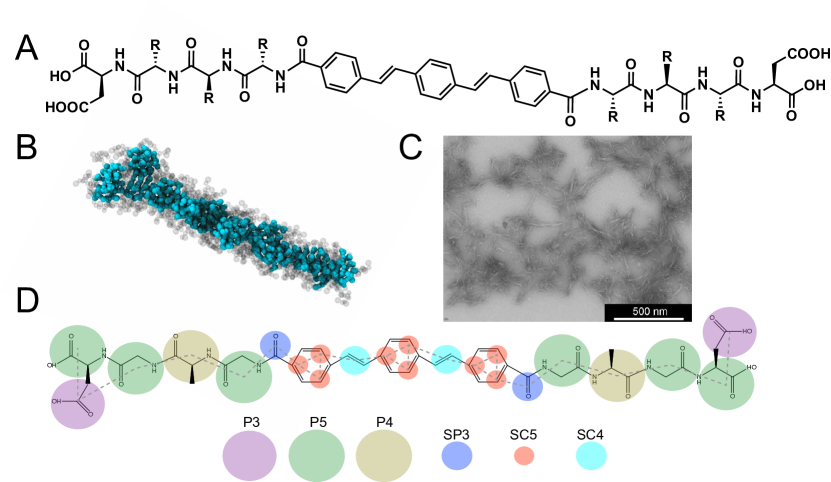
Figure 1: The DXXX-OPV3-XXXD system. (a) Chemical structure of the prototypical DXXX-OPV3-XXXD peptide monomer. The oligophenylenevinylene $\pi$ core (OPV3) is flanked by oligopeptide wings (DXXX) that are mirror symmetric such that the identity of the amino acids is inverted and the molecule possesses two C-termini. The X residues are selected from the 20 natural amino acids such that the family comprises 20³ = 8,000 distinct molecules. (b) Molecular simulation snapshot of a self-assembled pseudo-1D nanoaggregate spontaneously formed by the spontaneous association of DVAA-OPV3-VAAD peptide monomers into a linear stack. Good stacking between the $\pi$-cores (colored blue) favors $\pi$ orbital overlap, electronic delocalization along the backbone of the nanoaggragate, and the emergence of optical and electronic functionality. (c) Experimental transmission electron microscopy (TEM) image of self-assembled fibrils formed by DFFG-OPV3-GFFD peptides in an acidic environment. Reprinted with permission from Ref. ²² . Copyright (2014) American Chemical Society. (d) Illustration of the mapping from the DGAG-OPV3-GAGD all-atom structure to the coarse-grained representation at which the simulations in this work are conducted. The coarse-grained beads corresponding to groupings of neighboring atoms are labeled according to the Martini model employed in this work ^{36, 37, 38}.

The complete DXXX-OPV3-XXXD family comprises 20³ = 8,000 members corresponding to all possible permutations of the 20 natural amino acids within the unspecified XXX triplet. This vast size of this chemical space is both a blessing – the large palette of molecular chemistries provides enormous versatility in materials properties and the opportunity to tailor structure and function – and a curse – it is a challenge to identify promising candidates within this enormous space. Identifying the candidates capable of self-assembling into well-ordered optoelectronic nanoaggregates and divining the design precepts dictating the mechanism is a key goal in realizing these peptides as novel biocompatible optoelectronic materials.

Edisonian traversal of the large chemical space of DXXX-OPV3-XXXD molecules by trial-and-improvement experimentation is essentially intractable due to the high time and labor costs associated with peptide synthesis and testing. To date, no more than 13 members of the family have been experimentally synthesized and tested ²². Molecular simulation offers an alternative means to perform high-throughput virtual screening of chemical space to identify the most promising candidates for experimental testing. Since assembly proceeds on length scales of tens of nanometers and microsecond time scales, this has motivated the development of coarse-grained models explicitly parameterized against all-atom molecular simulations ^{17, 29, 39} (Fig. 1d). These models integrate out the electronic and atomistic degrees of freedom by lumping together small numbers of atoms into beads in order to furnish a molecular model that offers a judicious compromise between chemical realism and the computational efficiency required to directly simulate peptide assembly ²⁹. Exhaustive simulation of all 8,000 candidates within the DXXX-OPV3-XXXD family remains, however, computationally expensive. As we shall demonstrate, however, doing so is unnecessary to parameterize a reliable surrogate model of peptide function and identify and validate the most promising candidates within the family.

Chemical intuition is extremely valuable in guiding the computational search through chemical space, but it can perform poorly in the limits of data paucity, where there are too few examples to infer patterns, and data abundance, where there are too many examples to parse effectively. Further, inherent preconceptions and biases may push the search away from potentially profitable regions of chemical space and overlook patterns in the high-dimensional data that may reveal important determinants of molecular performance. Active learning (a.k.a. sequential learning, optimal experimental design), and more specifically, Bayesian optimization, presents a systematic approach to guide traversal of chemical space by using information on all measurements conducted to date to inform the “next-best” measurement to conduct ^{40, 41, 42, 43, 44}. In this manner, active learning predicts an optimal sequence in which to consider the molecular candidates in order to identify the optimal ones with minimal data collection effort. For this reason, active learning and allied approaches have been rapidly gaining traction in the materials discovery, engineering, and design communities, with these approaches being deployed, for example, in the experimental discovery of novel shape memory alloys ⁴⁵, piezoelectrics ⁴⁶, high glass transition polymers ⁴⁰, the computational discovery of drugs ⁴³, and magnetocaloric, superconducting, and thermoelectric materials ⁴¹.

Our primary goal is to efficiently identify members of the DXXX-OPV3-XXXD family that exhibit self-assembly into desired pseudo-1D nanoaggregates with good overlap between the $\pi$-conjugated cores and are thus most promising in displaying emergent optical and electronic functionality. We adopt a coarse-grained bead-level molecular simulation model as the engine for our high-throughput virtual screen and couple this with a deep learning-enabled active learning protocol to guide optimal traversal of chemical space. We identify and computationally validate the top performing constituents of the 8,000-member DXXX-OPV3-XXXD family after simulating only 2.3% of all possible molecules. This represents a massive saving over exhaustive sampling enabled by active learning. The absence of any introduced human bias within the active learning protocol also proved to be valuable in identifying high-performing candidates incorporating methionine residues that were not previously considered. A post hoc analysis of the observed assembly pathways provides supporting mechanistic understanding of the self-assembly behavior and exposes practical precepts for molecular design. The rank ordered list of DXXX-OPV3-XXXD molecules produced by our computational analysis provides a useful filtration of the design space with the top-performing candidates offering a massively reduced candidate space for experimental synthesis and testing.

2 Methods

2.1 Molecular dynamics simulation

The DXXX-OPV3-XXXD peptides were modeled using a previously-developed coarse-grained potential based on the Martini potential ^{29, 17}. Martini is a popular coarse-grained potential that lumps approximately four heavy atoms into each coarse-grained bead, has demonstrated great successes in modeling peptides, proteins, lipids, and carbohydrates ^{37, 38, 47, 48, 49, 50, 51}, and offers a good compromise between chemical specificity and the computational efficiency necessary to probe the formation of large peptide aggregates. The potential was initially developed for DFAG-OPV3-GAFD by refitting the native Martini parameters for bonded interactions against all-atom simulation data ²⁹. This bottom-up reparameterization of the bonded interactions greatly improved agreement between the coarse-grained and all-atom distribution functions, potentials of mean force (PMF) for monomer stretching and dimerization, and time-averaged contact maps ²⁹. We generalize this model to the complete DXXX-OPV3-XXXD family by maintaining the same parameterization of the bonds, angles, and backbone dihedrals within the OPV3 core and employing default Martini parameters for the amino acid side chains and all non-bonded interactions ^{36, 38}. An illustration of the all-atom to coarse-grained bead-level mapping for DGAG-OPV3-GAGD is provided in Fig. 1d. Calculation and comparison of the translational diffusion constants for the all-atom and coarse-grained models of DFAG-OPV3-GAFD showed these to be in agreement within error bars, indicating no significant discrepancy in the (translational) dynamical time scales between the two models and that no time scale corrections to the coarse grained calculations are required.

Coarse-grained molecular dynamics simulations of peptide assembly were conducted using the Gromacs 2018.6 simulation suite ⁵². Initial system configurations for each DXXX-OPV3-XXXD considered were generated by randomly inserting 96 peptides into a 16.2$\times$16.2$\times$16.2 nm³ cubic simulation box with 3D periodic boundary conditions, corresponding to a concentration of approximately 35 mM. The amino acid residues are prepared in protonation states corresponding to pH 1 to mimic pH-triggered experimental assembly under acidic conditions. The coarse-grained peptides were then solvated in water to a density of 1.0 g/cm³ of water using the Martini non-polarizable water model ³⁶. Steepest descent energy minimization was performed to eliminate high energy overlaps by removing forces greater than 1,000 kJ/mol.nm. Initial particle velocities were assigned from a Maxwell-Boltzmann distribution at 298 K. All simulations were conducted in the NPT ensemble at 298 K and 1 bar using a velocity-rescaling thermostat ⁵³ and Parrinello-Rahman barostat ⁵⁴. Equations of motion were numerically integrated using the leap-frog algorithm with a 5 fs time step ⁵⁵ and bond lengths fixed using the LINCS algorithm ⁵⁶. Lennard Jones interactions were smoothly shifted to zero at 1.1 nm and reaction-field electrostatics were employed using a relative electrostatic screening constant of 15 appropriate for the non-polarizable water model ³⁷. An initial 100 ps equilibration run was conducted, after which time the temperature, pressure, density, and energy all stabilized. This was followed by a 3 $\mu$s production run, after which time the structural evolution of the system as measured by graphical analysis of the self-assembled aggregate (see Section 2.2.1) was stationary in time. Simulation snapshots were harvested for analysis every 50 ps over the course of the production run. Calculations were predominantly conducted on single NVIDIA GeForce RTX 2080 Ti cards and achieved execution speeds of $\sim$1.45 $\mu$s/day.

2.2 Active learning peptide discovery

An active learning protocol is employed to direct a principled traversal of the DXXX-OPV3-XXXD candidate space and minimize the number of coarse-grained simulations required to discover the highest-performing candidates ^{40, 41, 42}. The fundamental challenge is that evaluating the quality of each peptide by direct simulation is expensive, so we wish to identify the best peptide candidates in the fewest number of simulations. The procedure we employ is in large part inspired by and adapted from a pioneering deep representational active learning approach for molecular drug discovery developed by Gomez-Bombarelli et al. ⁴³. Our approach comprises four main steps and is illustrated schematically as an iterative active learning cycle in Fig. 2. The coarse-grained molecular simulation engine representing our measurement function within the protocol is described in Section 2.1, and we define our fitness function in Section 2.2.1. Appreciating that some of the more technical machine learning concepts may be foreign to some readers in the molecular modeling community, we expose these steps in the protocol in some detail along with their specific adaptations to our molecular system, but those readers familiar with variational autoencoders, Gaussian process regression, and Bayesian optimization may feel free to skim over Sections 2.2.2-2.2.6. All codes are developed in Python 3 making use of the Scikit-learn ⁵⁷, NumPy ⁵⁸, Keras ⁵⁹, and ORCA ⁶⁰ libraries. Jupyter notebooks implementing our methods are hosted on GitHub (https://github.com/KirillShmilovich/ActiveLearningCG).

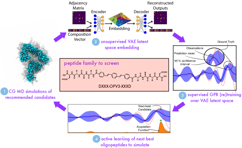
Figure 2: Active learning cycle for the data-driven discovery of optimally self-assembling DXXX-OPV3-XXXD peptides. The cycle contains four components. (1) Coarse-grained molecular simulations are performed on selected DXXX-OPV3-XXXD candidates and the quality of the self-assembled aggregates formed by molecule $i$ measured according to a scalar fitness $f_{i}$. (2) The DXXX-OPV3-XXXD family is projected from the high-dimensional chemical space of molecular structures into a low-dimensional latent space embedding $E:\text{DXXX-OPV3-XXXD}_{i}\rightarrow\mathbf{z}_{i}\in\mathbb{R}^{d}$ using a variational autoencoder (VAE). The dimensionality of the latent space is optimized during each cycle. (3) A Gaussian process regression (GPR) model is constructed over the VAE latent space linking the latent space coordinates of each DXXX-OPV3-XXXD family member to the scalar fitness function measuring the quality of their self-assembled aggregates $f:\hat{f}_{i}=f(\mathbf{z}_{i})=(f\circ E)(\text{DXXX-OPV3-XXXD}_{i})$. The GPR mapping $f$ is retrained each cycle over all DXXX-OPV3-XXXD candidates that have been simulated to date and for which measures of the fitness function $f_{i},\;i\in sampled$ is available, and is then used to predict the fitness of unsimulated candidates $\hat{f}_{j},\;j\in unsampled$. (4) The predicted means and uncertainties for $\hat{f}_{j},\;j\in unsampled$ furnished by the GPR surrogate model are combined within an active learning acquisition function to identify the “next-best” candidates for which to perform coarse-grained molecular simulations to drive sampling towards the most promising candidates. The loop is cycled until the GPR surrogate model no longer changes with additional data collection and can then be used to reliably identify the top candidates for computational validation.

2.2.1 Step 1: Definition of fitness function for self-assembled aggregates

To perform active learning discovery in our predefined chemical space we define a scalar-valued fitness function $f:f_{i}=f(\text{DXXX-OPV3-XXXD}_{i})$ that assigns a quality to each peptide in terms of its capacity to self-assemble into pseudo-1D nanoaggregates. Linear aggregates with good overlap between the $\pi$-conjugated cores are most promising in displaying emergent optical and electronic functionality and therefore anticipated to possess the most desirable materials properties. We have previously employed DFT calculations to make direct predictions of optoelectronic properties, but the high computational cost of these calculations limit them to aggregates of small numbers of peptides (dimers and trimers) and require omission of the flanking amino acid residues and solvent ²⁸. As such, these calculations are poorly suited to high-throughput virtual screening for large-scale aggregation behavior. Consequently, we define and optimize a structural measure of assembly quality in our coarse-grained molecular simulations as a proxy for optical and electronic functionality. This simplification massively expedites sampling in the full chemical space and provides a means to coarsely screen chemical space and focus a subsequent experimental search on the most promising candidates. Alternatively, this computational screen can be viewed as a preliminary filtration within the coarsest level of a nested hierarchy of increasingly expensive all-atom and/or electronic structure calculations.

In order to specify $f$ we define a geometric criterion by which a pair of peptides are considered to form part of the same pseudo-1D nanoaggregate. To do so, we adopt a distance metric that we have previously employed to define clustering in DFAG-OPV3-GAFD assembly ^{29, 17} and asphaltene aggregation ⁶¹. This so-called “optical distance” metric is defined as the minimum center of mass distance between aromatic cores in molecule $a$ and $b$,

$$d^{\text{optical}}_{ab}=\min_{i\in core(a),j\in core(b)}r_{ij},$$ (1)

where $r_{ij}$ is the intermolecular center-of-mass distance between the aromatic rings $i$ and $j$ within the OPV3 cores, and the minimization proceeds over the three aromatic rings $i\in core(a)$ in molecule $a$, and the three aromatic rings $j\in core(b)$ in molecule $b$. Pairs of molecules $a$ and $b$ which satisfy $d^{\text{optical}}_{ab}<r_{\text{cut}}=0.7$ nm are considered to reside within the same cluster ^{29, 17}. The cutoff $r_{\text{cut}}=0.7$ was tuned to the mean of the distribution of $d^{\text{optical}}_{ab}$ collected over DFAG-OPV3-GAFD peptide dimers with good in-register stacking of the OPV3 cores ²⁹. In contrast with other choices of peptide clustering metrics based, for example, on the overall center-of-mass or proximity of the peptide wings, the optical metric assures close intermolecular proximity of at least one pair of OPV3 aromatic rings in a pair of associated peptides. This close association promotes $\pi$ electron overlap, electron delocalization, and the emergence of optoelectronic function, and it is for this reason that this metric is termed the optical distance metric ^{29, 39, 17}.

Given this definition, a natural choice for the fitness $f_{i}$ of molecule $i$ is the number of such optical contacts in a self-assembled aggregate, since maximizing this value will promote electronic delocalization and the emergence of optoelectronic functionality. We evaluate the fitness function by representing the molecular system as a dynamically-evolving interaction graph in which the peptides compose the vertices $V=\{v_{1},v_{2},\ldots,v_{N}\}$ and the edges $E=\{e_{1,2},e_{1,3},...,e_{95,96}\}$ are assigned between pairs of vertices $v_{a}$ and $v_{b}$ if $d^{\text{optical}}_{ab}<r_{\text{cut}}=0.7$. An illustration of the evolution of the interaction graph over the course of a 3 $\mu$s simulation of DDAI-OPV3-IADD assembly is presented in Fig. 3. The number of vertices $|V|$ = 96 is fixed by the number of peptides in the system. Maximization of the number of edges $|E(t)|$ at time $t$ is therefore equivalent to maximizing the mean degree of each vertex in the graph $\kappa(t)=\frac{2|E(t)|}{|V|}$. As such, we adopt as our fitness function,

$$f_{i} =\overline{\kappa(t;\text{DXXX-OPV3-XXXD}_{i})}=\frac{2\overline{|E(t;\text{DXXX-OPV3-XXXD}_{i})|}}{|V|},$$ (2)

where the time average denoted by the overbar is performed over the terminal 50 ns of the 3 $\mu$s production run. Standard errors in the mean are estimated by block averaging the terminal 50 ns in five contiguous 10 ns blocks.

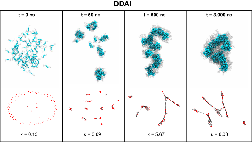
Figure 3: Dynamical evolution of the self-assembled structures of DDAI-OPV3-IADD over the course of a 3 $\mu$s coarse-grained molecular simulation. Snapshots of the molecular simulation show molecules in which the OPV3 $\pi$ cores are colored blue, the peptide wings faded grey, and water is removed for clarity. The interaction graph corresponding to each snapshot is shown directly below each image. The vertices $V$ corresponding to each peptide are colored red, and edges $E$ between peptide pairs defined by $d^{\text{optical}}_{ab}<r_{\text{cut}}=0.7$ (Eqn. 1) and colored grey. The average degree $\kappa=\frac{2|E|}{|V|}$ is reported at the bottom of each panel. At $t$ = 0 ns, the 96 randomly placed peptides form essentially a monomeric dispersion, with the exception of five dimer pairs, and the system possesses a correspondingly low $\kappa$ = 0.13. As the simulation progresses, the peptides self assemble under the influence of hydrogen bonding, $\pi$-$\pi$ stacking, and hydrophobic interactions into small ($t$ = 50 ns, $\kappa$ = 3.69) and then larger ($t$ = 500 ns, $\kappa$ = 5.67; $t$ = 3,000 ns, $\kappa$ = 6.08) aggregates with a commensurate increase in the mean degree $\kappa$. In this figure, and throughout the paper, molecular renderings are generated using VMD ⁶², and interaction graphs produced using NetworkX ⁶³.

A potential criticism of the fitness function is that $\kappa$ achieves a maximum for all-to-all connectivity of the graph, and its maximization would therefore appear to not necessarily favor pseudo-1D linear stacks. Mathematically this is true, but there are strong physical limitations on the maximum attainable value of $\kappa$ since the excluded volume of the $\pi$ cores allow then to form optical associations with a limited number of partners. The largest value observed in all of our calculations is $\kappa$ = 6.07 (cf. Table 1), and visual inspection of the terminal aggregates confirms that $\kappa$ is positively correlated with the formation of elongated pseudo-1D nanoaggregates similar to those illustrated in the $t$ = 3,000 ns panel of Fig. 3.

2.2.2 Step 2: Learning latent space embeddings using variational autoencoders

In Step 3 (Section 2.2.3) we describe our training of a Gaussian process regression (GPR) surrogate model to predict the fitness of candidate molecules that have not been simulated based on those that have. The predictions of this model are then used to perform active learning. We experimented with constructing the GPR directly over the chemical space of DXXX-OPV3-XXXD molecules by measuring pairwise distances between the XXX tripeptides using BLOSUM substitution matrices ⁶⁴, but following Gomez-Bombarelli et al. ⁴³, we found this approach to yield inferior surrogate models to those constructed over data-driven low-dimensional embeddings of the molecules generated using a variational autoencoder (VAE) ⁶⁵. The low-dimensional VAE latent spaces also conveys advantages in that low-dimensional GPRs tend to be more robust, chemically similar molecules tend to be embedded proximately in the latent space providing interpretability of the chemical space through dimensionality reduction, and the continuous and differentiable nature of the latent space makes it well-suited to global optimization ^{43, 66}.

We represent the DXXX-OPV3-XXXD molecules to the VAE only through the identity of the XXX tripeptide, since this is the only differentiating feature between molecules. We base this representation on the coarse-grained Martini model used to perform our molecular simulations. This representation comprises two components for each molecule $i$: (i) an adjacency matrix $\mathbf{A}_{i}$, which captures the connectivity of beads within the tripeptide, and (ii) a one-hot encoded composition vector of bead-types $\mathbf{T}_{i}$ specifying the identity of the Martini beads (Fig. 4). Since peptide sequences may contain varying numbers of coarse-grained beads, we standardize the size of the adjacency matrix $\mathbf{A}_{i}\in\mathbb{R}^{15\times 15}$ to be sufficiently large enough to accommodate the largest tripeptide (Trp-Trp-Trp) and pad the array with zeroes for smaller molecules. A one-hot composition vector of length $\mathbf{T}_{i}\in\mathbb{R}^{75}$ is sufficient to accommodate all tripeptide compositions considered. For each molecule $i$, the tuple $(\mathbf{A}_{i},\mathbf{T}_{i})$ defines the input provided to the VAE.

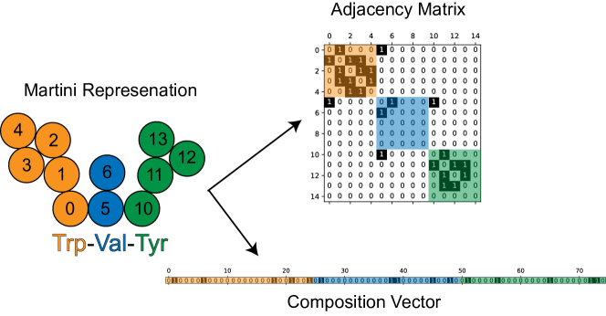
Figure 4: Schematic of the representation of each XXX tripeptide to the VAE. The Martini representation of each tripeptide $i$, in this example Trp-Val-Tyr (WVY), is converted into an adjacency matrix $\mathbf{A}_{i}\in\mathbb{R}^{15\times 15}$ specifying the connectivity of beads within the tripeptide and a one-hot composition vector $\mathbf{T}_{i}\in\mathbb{R}^{75}$ specifying the identity of the beads. The tuple $(\mathbf{A}_{i},\mathbf{T}_{i})$ defines the input provided to the VAE. A pre-defined sequential numbering is employed for the beads in each amino acid. The adjacency matrix is padded with rows and columns of zeros to represent tripeptides containing fewer than the maximum number of 15 beads. The colored blocks in the adjacency matrix and composition vector correspond to the colors of the amino acids in the Martini molecule.

The architecture of the VAE is illustrated in Fig. 5. Given the two-part input $(\mathbf{A}_{i},\mathbf{T}_{i})$ for molecule $i$, the encoder block processes this through two parallel networks to perform feature extraction from each input. The $\mathbf{A}_{i}$ resemble a small image which motivate using a short series of convolutional layers to treat these inputs, whereas the binary $\mathbf{T}_{i}$ vectors are passed through a series of fully-connected dense layers. The features extracted by the encoder through the two parallel encoder networks are subsequently concatenated and used to generate the mean $\boldsymbol{\mu}_{i}$ and standard deviation $\boldsymbol{\sigma}_{i}$ of a Gaussian distributed latent space embedding $\mathbf{z}_{i}\sim\mathcal{N}(\boldsymbol{\mu}_{i},\boldsymbol{\sigma}_{i})\in\mathbb{R}^{d}$. The dimensionality of the latent space is treated as a hyperparameter that is optimized during each cycle of active learning and is found to lie in the range $d\in[4,10]$. The decoder then attempts to reconstruct $(\mathbf{A}_{i},\mathbf{T}_{i})$ from the latent encoding $\mathbf{z}_{i}$ again using two parallel networks. The part of the decoder predicting the reconstruction $\hat{\mathbf{T}}_{i}$ is identical to the architecture of the encoder, whereas the part predicting the reconstruction $\hat{\mathbf{A}}_{i}$ is simply another series of fully-connected layers that is reshaped to match the size of the input. The overall action of the VAE is the functional composition of the encoder $E:\mathbf{z}_{i}=E(\mathbf{A}_{i},\mathbf{T}_{i})$ and decoder $D:(\hat{\mathbf{A}}_{i},\hat{\mathbf{T}}_{i})=D(\mathbf{z}_{i})$ blocks such that the total effect of the network is $(\hat{\mathbf{A}}_{i},\hat{\mathbf{T}}_{i})=(D\circ E)(\mathbf{A}_{i},\mathbf{T}_{i})$.

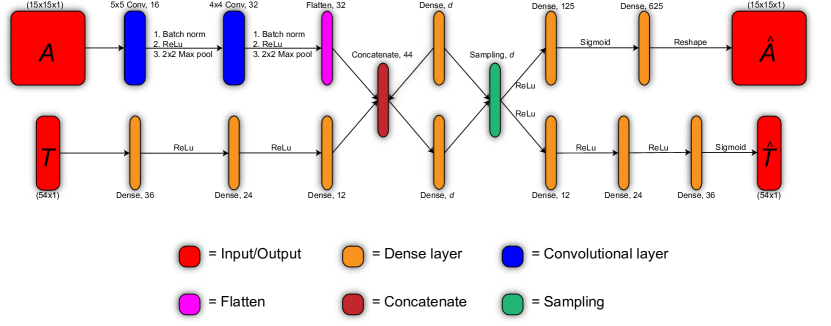
Figure 5: Architecture of the variational autoencoder (VAE) used to generate the DXXX-OPV3-XXXD latent space embedding. The VAE accepts as inputs adjacency matrix and composition vector tuples $(\mathbf{A}_{i},\mathbf{T}_{i})$ and employs two parallel encoders to perform feature extraction and learn the mean $\boldsymbol{\mu}_{i}$ and standard deviation $\boldsymbol{\sigma}_{i}$ of a Gaussian distributed latent space embedding $\mathbf{z}_{i}\sim\mathcal{N}(\boldsymbol{\mu}_{i},\boldsymbol{\sigma}_{i})\in\mathbb{R}^{d}$. The decoder generates approximate reconstructions $(\hat{\mathbf{A}}_{i},\hat{\mathbf{T}}_{i})$ of the inputs from the latent space representation. The network is trained by minimizing a loss function balancing reconstruction accuracy and a regularization term constraining the latent space to follow a multidimensional Gaussian distribution (Eqn. 3). The dimensionality $d$ of the latent space is treated as a hyperparameter that is optimized during each cycle of active learning.

The VAE is trained by minimizing the VAE loss $\mathcal{L}_{VAE}$ composed of a reconstruction term $\mathcal{L}_{Rec}$ and a Kullback-Leibler (KL) divergence term $\mathcal{L}_{KL}$ ^{65, 67},

$$\mathcal{L}_{VAE} =\mathcal{L}_{Rec}+\mathcal{L}_{KL},$$ (3)

$$\mathcal{L}_{Rec} =\mathbb{E}_{i}[\text{BCE}(\hat{\mathbf{A}}_{i},\mathbf{A}_{i})+\text{BCE}(\hat{\mathbf{T}}_{i},\mathbf{T}_{i})])$$

$$\approx\sum_{i\in\text{mini-batch}}[\sum_{j=1}^{15}(A_{i,j}\log(\hat{A}_{i,j})+(1-A_{i,j})\log(1-\hat{A}_{i,j}))$$

$$\qquad+\sum_{j=1}^{75}(T_{i,j}\log(\hat{T}_{i,j})+(1-T_{i,j})\log(1-\hat{T}_{i,j}))],$$ (4)

$$\mathcal{L}_{KL} =-D_{KL}(\mathbf{z}=E(\mathbf{A},\mathbf{T})~{}||~{}\mathcal{N}(0,\mathbf{I}))$$

$$\approx\sum_{i\in\text{mini-batch}}[-\frac{1}{2}\sum_{j=1}^{d}(1+\log(\sigma_{i,j}^{2})-\sigma_{i,j}^{2}-\mu_{i,j}^{2})],$$ (5)

where $\text{BCE}(\mathbf{x},\mathbf{y})$ is the binary cross entropy between the reconstructions $\mathbf{x}$ and ground truth $\mathbf{y}$, $D_{KL}(Q~{}||~{}P)$ is the Kullback-Leibler divergence from $P$ to $Q$, and $\mathbf{I}$ is the $n$-by-$n$ identity matrix. The reconstruction term $\mathcal{L}_{Rec}$ encourages the VAE to reconstruct the inputs through the low-dimensional latent space information bottleneck. In contrast to a vanilla autoencoder which only aims to minimize $\mathcal{L}_{Rec}$, the KL divergence term $\mathcal{L}_{KL}$ is an effective regularizer which imposes a multivariate Gaussian prior on the latent space and prevents the VAE from essentially “memorizing” the data set and learning a trivial identity mapping through a disconnected latent space ⁶⁷. Training is performed by passing tuples $(\mathbf{A}_{i},\mathbf{T}_{i})$ through the VAE in mini-batches of size 32 and updating the network parameters with mini-batch gradient descent using the Adam optimizer ⁶⁸. The VAE loss $\mathcal{L}_{VAE}$ is typically observed to plateau within 4,000 epochs. We note that the regularization introduced by the KL divergence term $\mathcal{L}_{KL}$ serves to prevent over-fitting and enables us to train over the full set of molecules to be embedded by the VAE.

We present in Fig. 6 an example of a $d$ = 3 VAE latent space embedding of the DXXX-OPV3-XXXD family. We color each member of the family by the number of beads in the XXX tripeptide to show that the first dimensional of the latent space $z_{1}$ is approximately correlated with molecular size, possessing a Pearson correlation coefficient $\rho(z_{1},\text{size})$ = 0.858 (p-value < 1$\times$$10^{-15}$). The other two dimensions in this example are also some functions of molecular composition and topology, but prove more challenging to correlate with physically interpretable observables. Physical interpretability of the latent space dimensions is a pleasing but not required property of the embedding. The primary purpose of the VAE embedding is to provide a smooth, low-dimensional molecular representations for the GPR surrogate model. We note that the latent space embedding could be shaped and made more interpretable by simultaneous training of a supervised regression model as suggested by Gomez-Bombarelli et al. ⁴³.

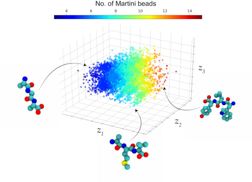
Figure 6: Illustrative visualization of $d=3$ VAE latent space embedding of the DXXX-OPV3-XXXD family. The embedded molecules are colored according to the number of beads in the XXX tripeptide and selected molecules are visualized. The first dimensional of the latent space $z_{1}$ is correlated with molecular size $\rho(z_{1},\text{size})$ = 0.858 (p-value $<$ 1$\times$$10^{-15}$) providing a visual illustration that similar molecules are embedded close together in the VAE latent space.

2.2.3 Step 3: Gaussian process regression surrogate models

Fitness measurements $f_{i},\;i\in sampled$ are available for those molecules DXXX-OPV3-XXXD_i for which we have performed coarse-grained molecular simulation. Given these data we wish to predict the fitness of all remaining candidates $\hat{f}_{j},\;j\in unsampled$. This constitutes a supervised regression task where we wish to train a surrogate model $f$ over a small number of training examples to predict the fitness of out-of-training examples as a function of their location in the VAE latent space: $f:\hat{f}_{i}=f(\mathbf{z}_{i})=(f\circ E)(\mathbf{A}_{i},\mathbf{T}_{i})$. In this manner, the regression model “short circuits” expensive direct simulation prediction of fitness with a cheap surrogate model, and eliminates the need to perform exhaustive calculations over all molecules in the family. The quality of the model predictions depends on the number and chemical similarity of the training data: the model is expected to perform better with larger training sets and make more accurate predictions for out-of-training examples that are chemically similar to examples in the training set. As such, we expect the model to improve with additional cycles around the active learning loop. For the purposes of active learning (Section 2.2.4), it is also vital to perform uncertainty quantification on the model predictions so that we can both direct sampling towards the most high-performing candidates predicted by the model (exploitation) and towards undersampled areas where the model possesses the highest uncertainties (exploration) ⁶⁹. For this reason, we select Gaussian process regression (GPR) to construct our surrogate model $f:\hat{f}_{i}=f(\mathbf{z}_{i})$ as a flexible, non-parametric, Bayesian regression approach that comes with built-in uncertainty estimates ^{70, 71, 72, 69}.

The fundamental principle of a GPR is to employ a Gaussian process to specify a Bayesian prior distribution over regression functions fitting the data, and then to compute the posterior distribution over those functions that are in agreement with the training data ⁷². The Gaussian process is fully specified by its mean function, which is typically defined to be zero, and its covariance function for which we choose the popular squared exponential kernel,

$$k(\mathbf{z},\mathbf{z}^{\prime})=\exp(-\frac{1}{2\gamma}||\mathbf{z}-\mathbf{z}^{\prime}||^{2}),$$ (6)

where $\mathbf{z}$ and $\mathbf{z}^{\prime}$ denote latent space vectors and the bandwidth of the kernel $\gamma$ is a hyperparameter defining the characteristic length scale over which latent space vectors “see” one another. Under these choices, the predicted fitness $f^{*}=f(\mathbf{z}^{*})$ for a new point $\mathbf{z}^{*}$ outside of the training data is a Gaussian distributed random variable with ^{72, 71},

$$f^{*} \sim\mathcal{N}(\mu_{f^{*}},\sigma_{f^{*}}),$$ (7)

$$\mu_{f^{*}} =K(\mathbf{z}^{*},\mathbf{Z})\left[K(\mathbf{Z},\mathbf{Z})+(\boldsymbol{\sigma}_{f}^{2})^{T}\mathbf{I}\right]^{-1}\mathbf{f},$$

$$\sigma_{f^{*}} =K(\mathbf{z}^{*},\mathbf{z}^{*})-K(\mathbf{z}^{*},\mathbf{Z})\left[K(\mathbf{Z},\mathbf{Z})+(\boldsymbol{\sigma}_{f}^{2})^{T}\mathbf{I}\right]^{-1}K(\mathbf{z}^{*},\mathbf{Z})^{T},$$

where $\mathbf{I}$ is the $n$-by-$n$ identity matrix, $\mathbf{f}=\left[f_{1},f_{2},\ldots,f_{n}\right]^{T}$ is the vector of (noisy) measurements of fitness for the $n$ training points $\mathbf{Z}=\{\mathbf{z}_{1},\mathbf{z}_{2},...,\mathbf{z}_{n}\}$ computed in our coarse-grained molecular simulations, and $\boldsymbol{\sigma}_{f}^{2}=\left[\sigma_{f_{1}},\sigma_{f_{2}},\ldots,\sigma_{f_{n}}\right]^{T}$ are associated variances of assumed i.i.d. Gaussian noise estimated by block averaging (Section 2.2.1), and the $K$ matrices hold the covariances within and between the training data $\mathbf{Z}$ and new point $\mathbf{z}^{*}$,

$$K(\mathbf{Z},\mathbf{Z}) =\begin{bmatrix}k(\mathbf{z}_{1},\mathbf{z}_{1})&k(\mathbf{z}_{1},\mathbf{z}_{2})&\cdots&k(\mathbf{z}_{1},\mathbf{z}_{n})\\ \vdots&\vdots&\ddots&\vdots\\ k(\mathbf{z}_{n},\mathbf{z}_{1})&k(\mathbf{z}_{n},\mathbf{z}_{2})&\cdots&k(\mathbf{z}_{n},\mathbf{z}_{n})\end{bmatrix},$$ (8)

$$K(\mathbf{z}^{*},\mathbf{Z}) =\left[k(\mathbf{z}^{*},\mathbf{z}_{1}),k(\mathbf{z}^{*},\mathbf{z}_{2}),\cdots,k(\mathbf{z}^{*},\mathbf{z}_{n})\right],$$ (9)

$$K(\mathbf{z}^{*},\mathbf{z}^{*}) =k(\mathbf{z}^{*},\mathbf{z}^{*}).$$ (10)

The $(\boldsymbol{\sigma}_{f}^{2})^{T}\mathbf{I}$ terms account for the uncertainty inherent in our measurements of $\mathbf{f}$ through an assumed Gaussian noise model ⁷¹. These terms can also be conceived as a Tikhonov (a.k.a. ridge or nugget) regularization of the $K(\mathbf{Z},\mathbf{Z})$ matrix that stabilizes its matrix inverse and is particularly useful when this matrix is ill-conditioned due to the close proximity of two or more training points in $\mathbf{Z}$ ⁷³. A corollary of this regularization is that the GPR posterior is not a perfect interpolator of the training data due to the presence of measurement noise, and we should anticipate residual discrepancies on the order of $\boldsymbol{\sigma}_{f}$ between the GPR predictions and the our measurements of $\mathbf{f}$. The predictive accuracy and robustness of the GPR is enhanced by the smooth, continuous, and low-dimensional nature of the VAE latent space, which embeds chemically similar points nearby one another and therefore promotes transfer of information to new out-of-training points based on chemically proximate training examples. The GPR prior and posterior are updated during each cycle of the active learning loop as additional training data are collected.

2.2.4 Step 4: Bayesian optimization

The final step in the cycle is to use the predictions of the surrogate GPR model to identify the next peptide candidates to simulate. We frame this active learning problem as a Bayesian optimization, where we have an expensive, non-differentiable, black-box function with noisy evaluations – the fitness of each molecule evaluated by coarse-grained molecular simulation – that we wish to optimize in the minimum number of evaluations. Bayesian optimization defines an acquisition function $u$ that wraps around the current surrogate model to identify peptides with a high chance of being better than the current leader in the training data. We can represent optimization of the acquisition function as,

$$\mathbf{z}^{\dagger} =\underset{\mathbf{z}}{\mathrm{argmax}}\;u(\mathbf{z}|\mathbf{Z}=\{(\mathbf{z}_{1},f_{1}),(\mathbf{z}_{2},f_{2})...,(\mathbf{z}_{n},f_{n})\}),$$ (11)

where $\mathbf{z}^{\dagger}$ is the VAE latent space coordinates of the DXXX-OPV3-XXXD molecule that maximizes the acquisition function $u$, and the maximization is conditioned on the $n$ samples $\{(\mathbf{z}_{1},f_{1}),(\mathbf{z}_{2},f_{2})...,(\mathbf{z}_{n},f_{n})\}$ collected to date. The surrogate model $f$ enters the maximization through the choice of acquisition function, for which many choices are available ⁶⁹. We employ the popular expected improvement (EI) acquisition function that provides a balanced trade-off between exploitation – selection of points where the surrogate model posterior mean $\mu_{f}(\mathbf{z})$ is large – and exploration – selection of points where the surrogate model posterior variance $\sigma_{f}(\mathbf{z})$ is large ^{74, 75, 69}. Following Lizotte, the EI is defined as ⁷⁶,

$$u(\mathbf{z}|\mathbf{Z})=\operatorname{EI}(\mathbf{z}|\mathbf{Z}) =\begin{cases}(\mu_{f}(\mathbf{z})-f(\mathbf{z}^{+})-\xi)\Phi(Z)+\sigma_{f}(\mathbf{z})\phi(Z)&\sigma_{f}(\mathbf{z})>0\\ 0&\sigma_{f}(\mathbf{z})=0\\ \end{cases},$$ (12)

$$Z =\begin{cases}\frac{\mu_{f}(\mathbf{z})-f(\mathbf{x}^{+})-\xi}{\sigma_{f}(\mathbf{z})}&\sigma_{f}(\mathbf{z})>0\\ 0&\sigma_{f}(\mathbf{z})=0\\ \end{cases},$$ (13)

where $f(\mathbf{z}^{+}),\;\mathbf{z}^{+}\in\mathbf{Z}=\{\mathbf{z}_{1},\mathbf{z}_{2},...,\mathbf{z}_{n}\}$ is the maximum fitness value among all $n$ sampled candidates to date, $\Phi$ and $\Psi$ are the cumulative distribution function and probability density function of the standard normal distribution, and the hyperparameter $\xi$ controls the exploration-exploitation trade-off. The first term in Eqn. 12 promotes exploitation and the second promotes exploration: when $\xi$ is small the EI will favor exploitation and select points with high posterior mean, while if $\xi$ is large exploration is performed selecting points with large posterior uncertainty ⁶⁹.

Active learning typically proceeds by selecting a fixed value $\xi$ = 0.01 ^{69, 76} of the exploration-exploitation trade-off, identifying the candidate that maximizes the EI, and then performing expensive function evaluation (here a coarse-grained molecular simulation) for that candidate. We employ a slightly modified version of this approach that effectively integrates over $\xi$ and performs active learning in batches, which has the advantages of (i) eliminating the sensitivity in selection to the hyperparameter $\xi$, (ii) spreading the exploit-explore trade-off, and (iii) making more efficient use of parallel compute resources to conduct multiple simulations in parallel in the same wall clock time. Specifically, we maximize the EI acquisition function over the range $\log_{10}\xi\in[-4,0.4]$ and select up to four candidates over this range as the “next-best” candidates to simulate. Molecules that have already been sampled in preceding rounds are excluded from the pool of available candidates at each round. Where more than four candidates emerge from the EI maximization, we randomly select four members of this set. An example of this selection procedure is presented in Fig. 7. Coarse grained molecular simulations of these optimal candidates are then performed to commence another round of the active learning cycle.

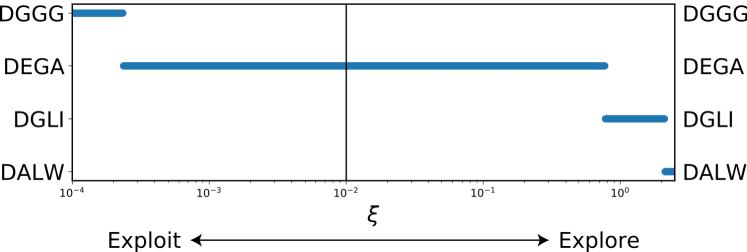
Figure 7: Active learning candidate selection. The expected improvement (EI) acquisition function (Eqn. 12) is evaluated over for all unsampled members of the DXXX-OPV3-XXXD family at values of the exploit-explore hyperparameter $\xi$ over the range $\log_{10}\xi\in[-4,0.4]$. The blue points in the graph indicate which DXXX candidate maximizes the EI at each value of $\xi$. In this illustrative example there are four candidates – DGGG, DEGA, DGLI, and DALW – that maximize the EI over the range of $\xi$ considered. The vertical line shows the recommended value of $\xi=0.01$ suggested in literature ^{69, 76}, which would result in the selection of only DEGA as the next molecule to simulate. In our approach, we select all four of the molecules DGGG, DEGA, DGLI, and DALW that maximize EI over the entire range of $\xi$ considered as the next best candidates to simulate in parallel in the next round of coarse-grained molecular simulations.

2.2.5 Hyperparameter optimization

The dimensionality $d$ of the VAE latent space embedding and bandwidth $\gamma$ of the GPR kernel are tunable hyperparameters to be optimized during each cycle of the active learning loop. We perform simultaneous tuning of $d$ and $\gamma$ during each round by creating 50 embeddings of all 8,000 DXXX-OPV3-XXXD molecules into the VAE latent space $\mathbf{z}_{i}\sim\mathcal{N}(\boldsymbol{\mu}_{i},\boldsymbol{\sigma}_{i})\in\mathbb{R}^{d}$, each employing different realization of random numbers to sample from the latent space Gaussian for each point, for $d$ = [3, 10]. We then optimize $\gamma$ for each embedding over the range $\gamma$ = [0.001, 100] using a line search followed by Nelder-Mead optimization to maximize the GPR accuracy under cross-validation. We employ leave-one-out cross-validation (LOO-CV) for the first five cycles of the active learning, and then 5-fold CV for subsequent rounds due to the high cost of LOO-CV for larger quantities of samples. The best performing VAE embedding and associated optimal $d$ and $\gamma$ are adopted for the remainder of the current active learning cycle.

2.2.6 Stop criteria

We cycle around the active learning loop until the GPR surrogate model no longer improves with the collection of additional training data. A number of stopping criterion for active learning have been proposed ^{77, 78, 79, 80, 81, 82}, but in this work we monitor and define convergence using the stabilizing predictions (SP) method that evaluates performance based on unlabeled data ⁸¹ and the performance difference (PD) method that considers the labeled examples ⁸³. The SP method examines the predictions of consecutive models at each iteration of the active learning procedure on a randomly selected set of 500 points, called the stop set, which is held constant throughout the active learning. We measure the difference in the regression predictions between subsequent rounds using the average Bhattacharyya distance $D_{B}$⁸⁴ between the posterior of consecutive GPR models over the stop set. Large differences in $D_{B}$ indicate the model is continuing to update the GPR posterior, whereas small values indicate that the surrogate model predictions have stabilized.

The PD method is used to evaluate model performance by 5-fold CV of the $R^{2}$ score over the accumulated labeled samples collected to date within each round of active learning. A plateau in the $R^{2}$ indicates that additional observations result in only marginal improvements to the GPR fit ⁸³. A caution in assessing convergence using labeled data is that these data may not be representative of the data as a whole ^{78, 85}. These concerns are mitigated in our application since our initial data set comprises a set of randomly selected peptides to initialize the active learning procedure and we collect up to four new data points each round across the exploit-explore spectrum to assure broad sampling of chemical space.

2.3 Nonlinear manifold learning of assembly pathways

We employ diffusion maps as a manifold learning approach to identify the low-dimensional assembly pathways by which the various DXXX-OPV3-XXXD molecules self-assemble into the terminal aggregates. We have previously described the application of diffusion maps to self-assembling systems in Refs. ^{86, 87, 61, 88}. In brief, we compute a distance metric $d(i,j)$ between each pair of interaction graphs $i$ and $j$ harvested from each frame of each molecular simulation trajectory. A number of graph kernels at varying levels of sophistication and abstraction have been proposed to measure the similarity between pairs of graphs ^{89, 90, 91, 92, 93}. We follow the approach of Reinhart et al. who employed graphlet decompositions as a diffusion map distance metric to analyze colloidal crystallization ⁹⁴. This approach featurizes a graph by enumerating all topologically unique subgraphs (“graphlets”) with associated node permutations (“orbits”) within the network up to a certain subgraph size (usually up to five vertices), and creating a vector of orbit counts for each vertex in our graph ^{60, 89, 94}. The vector of orbit counts at each vertex is reweighted to account for over-counting of the smaller graphlets contained in the larger ones (i.e. counts of graphlets comprising two vertices are necessarily contained in counts of graphlets comprising three or more vertices), averaged over all vertices in the graph, and normalized to unit length. This vector represents a featurization of the graph that is permutationally invariant to vertex labeling, and the L2-norm between pairs of vectors defines the graph kernel $d(i,j)$ used to evaluate pairwise distances between our graphical representations of the configurational state of the molecular system.

Diffusion maps then proceed by applying a Gaussian kernel to construct the convolved similarity matrix,

$$A_{i,j}=\exp\left(\frac{-\left(d(i,j)^{\alpha}\right)^{2}}{2\epsilon}\right),$$ (14)

where the kernel bandwidth $\epsilon$ controls the hop size of the random walk and can be automatically tuned based on the distribution of the $A_{i,j}$ ^{95, 61, 87}. The use of the hyperparameter $\alpha\in(0,1]$ was proposed by Wang et al. within a density-adaptive extension of diffusion maps that greatly improves the performance of diffusion maps in applications to systems with large differences in the density of points in the high-dimensional space ⁹⁶. For $\alpha$ = 1 we recover standard diffusion maps; for $\alpha\rightarrow 0$ the pairwise distances become increasingly similar and large fluctuations in the density of points in the high-dimensional space are smoothed out. Adopting the tuning procedure proposed in Ref. ⁹⁶ we adopt $\alpha$ = 0.15.

The $\bf{A}$ matrix is row normalized to create the right stochastic Markov transition matrix,

$$\bf{M}=\bf{D}^{-1}\bf{A},$$ (15)

Where $\bf{D}$ is a diagonal matrix of the row sums of $\bf{A}$.

$$D_{i,j}=\sum_{j=1}^{N}A_{i,j}.$$ (16)

The matrix element $M_{i,j}^{t}=p_{t}(i,j)$ can interpreted as the probability $p_{t}(i,j)$ of hopping from point $i$ to point $j$ in $t$ steps of the discrete random walk ^{95, 97}. Diagonalization of $\bf{M}$ produces an ordered set of eigenvectors and eigenvalues $\{(\psi_{1}=\vec{1},\lambda_{1}=1),(\psi_{2},\lambda_{2}),(\psi_{3},\lambda_{3}),...\}$ with $\lambda_{1}=1\geq\lambda_{2}\geq\lambda_{3}\geq\ldots$. The first pair $(\psi_{1}=\vec{1},\lambda_{1}=1)$ is trivial and associated with the stationary distribution of the random walk ⁹⁵. The higher order eigenvectors are associated with a hierarchy of increasingly fast relaxation modes of the random walk. Dimensionality reduction is achieved by identifying a gap in the eigenvalue spectrum after the $\lambda_{k+1}$ to resolve a subspace of slowly relaxing dynamical modes $\{\psi_{2},\psi_{3},\ldots,\psi_{k+1}\}$. The diffusion map embedding is the projection of the $i^{\text{th}}$ interaction graph into the $i^{\text{th}}$ component of the top $k$ non-trivial eigenvectors,

$$i\mapsto(\psi_{2}(i),\psi_{3}(i),...,\psi_{k+1}(i)).$$ (17)

We implement this formalism using the memory and compute efficient pivot diffusion map approach that reduces the scaling in the number of points $N$ from $\mathcal{O}(N^{2})$ to $\mathcal{O}(N\times n)$, where $n<<N$ is the number of so-called “pivot points” employed ⁹⁸. This approach enables the application of diffusion maps to large data sets by performing on-the-fly definition of the $n$ pivot points defining an approximate spanning tree over the high-dimensional data and which are used to support interpolative embeddings of the remaining points.

3 Results and Discussion

3.1 Active learning identification of optimal candidates

The complete DXXX-OPV3-XXXD family comprises 20³ = 8,000 members generated by all permutations of placing each of the 20 natural amino acids within the XXX tripeptide. Prior to conducting active learning we filtered this ensemble to eliminate a subset of candidates containing amino acids known and expected to produce undesired assembly behaviors ³⁹. Specifically, we reduced our search space to the 11³ = 1331 candidates in the set defined by $X\in\{\text{Ala},\text{Gly},\text{Glu},\text{Ile},\text{Leu},\text{Met},\text{Phe},\text{Trp},\text{Tyr},\text{Val},\text{Asp}\}$ to avoid charged and/or polar amino acids expected to interfere with low-pH triggered assembly ³¹ and focus on those residues that have expressed good assembly behavior in previous experimental work ^{22, 99, 100, 101}.

We perform active learning over DXXX-OPV3-XXXD sequences following the four-part protocol – molecular simulation, VAE latent space embedding, GPR surrogate model construction, optimal selection of next candidates – described in Section 2.2 and illustrated in Fig. 2. We seeded the search by conducting coarse-grained molecular dynamics simulations of 90 randomly selected members of the family using the simulation protocol detailed in Section 2.1. This initial broad sampling over the candidate space provides the GPR surrogate model with diverse training data that enables it to identify more- and less-promising regions of the latent space prior to making any predictions. We term this initial round of active learning as Round 0. We conduct 25 additional rounds of active learning (Rounds 1-25) selecting up to four additional molecules for simulation during each pass. This resulted in a sampling a total of $N$ = 186 molecules (2.3% of the 8,000-member complete family; 14.0% of the 1331-member chemically restricted family) and a cumulative 558 $\mu$s of simulation time. The particular candidates selected and sampled in each round are listed in Table S1 in the Supplementary Information.

Sampling was terminated by tracking the performance difference (PD) and stabilizing predictions (SP) methods (Section 2.2.6) ^{81, 83}. The PD method 5-fold cross validation $R^{2}$ score commences at a reasonably high value of $\sim$68% – likely due to the relatively large and diverse $N$ = 90 initial candidates considered, and plateaus to a quite high value of $\sim$78% by Round 18 (Fig. 8a). The SP method reveals a Bhattacharyya distance between successive GPR posteriors of $D_{B}$ > 10 over the first 13 rounds, indicating that the additional training data incorporated into the GPR surrogate model are substantially altering its predictions. After Round 14, the Bhattacharyya distance plateaus to $D_{B}$$\sim$ 2.5 indicating that the surrogate model has stabilized. Rounds 18-25 are therefore proceeding with a stable GPR model and the exploitation candidates identified by the expected improvement acquisition function (Section 2.2.4) furnish the best predictions of the top performing molecules that did not happen to have already been sampled in previous rounds.

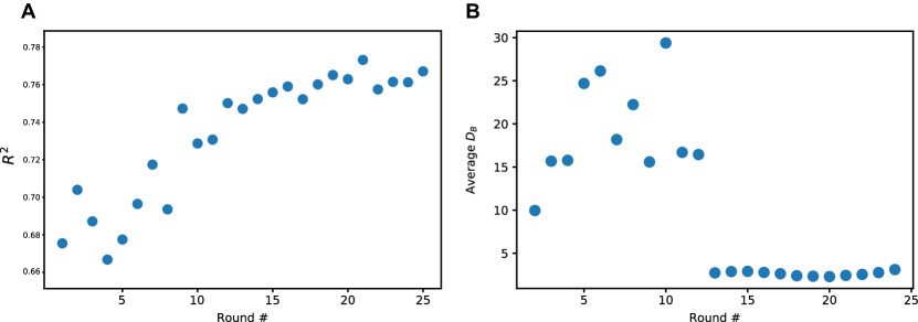
Figure 8: Tracking of active learning stop criteria. (a) The performance difference (PD) method 5-fold cross validation $R^{2}$ score stabilizes at $R^{2}$ $\sim$ 78% by Round 18. (b) The stabilizing predictions (SP) method Bhattacharyya distance between successive GPR posteriors plateaus close to zero at $D_{B}$ $\sim$ 2.5 after Round 13. Values are reported using a moving average with a window size of three, as recommended in Ref. ⁸¹ .

We present in Table 1 the top performing molecules among the 186 that were simulated within our active learning protocol. We report their fitness $f_{i}=\overline{\kappa}_{i}$ corresponding to the mean number of $\pi$-core–$\pi$-core contacts per molecule in the terminal self-assembled aggregates (Section 2.2.1), the round of active learning in which they were sampled, and whether they have been previously explored by experiment or simulation. Additional molecules that have been previously identified as high performing by experiment and simulation are also presented for comparison. The list of all 1,331 DXXX-OPV3-XXXD molecules in the family with fitness predictions and rankings assigned by the terminal GPR surrogate model is presented in Table S2. There is very good agreement between the numerical simulation results and the GPR model predictions over the training set of 186 molecules for which measurement data exist: the calculated and predicted values of $f_{i}=\overline{\kappa}_{i}$ possess a Pearson correlation coefficient of $\rho_{\text{Pearson}}$ = 0.90 (p-value = 4$\times$$10^{-68}$) and the calculated and predicted rankings possess a Spearman correlation coefficient of $\rho_{\text{Spearman}}$ = 0.86 (p-value = 1$\times$$10^{-54}$). The agreement is not perfect due to our incorporation of uncertainty estimates in our noisy fitness measurements into GPR training such that the model predictions fall within the error bars of our simulations (Section 2.2.3).

Table 1: Top 15 DXXX-OPV3-XXXD molecules identified by the active learning protocol. Additional molecules previously studied in simulation and experiment are also shown for comparison.

Rank (out of 186)	Molecule (DXXX)	$\overline{\kappa}$	Discovery round	Previously known?
1	DEAA	6.06 $\pm$ 0.02	1	N
2	DDAI	6.03 $\pm$ 0.02	0	N
3	DIAM	6.01 $\pm$ 0.02	17	N
4	DVAA	5.95 $\pm$ 0.03	9	N
5	DAAV	5.92 $\pm$ 0.03	19	N
6	DGLG	5.92 $\pm$ 0.02	20	N
7	DAEA	5.92 $\pm$ 0.02	25	N
8	DAGI	5.90 $\pm$ 0.01	21	N
9	DGIG	5.88 $\pm$ 0.02	25	N
10	DEAL	5.88 $\pm$ 0.01	23	N
11	DGGM	5.87 $\pm$ 0.04	0	N
12	DLAV	5.86 $\pm$ 0.02	16	N
13	DGDL	5.85 $\pm$ 0.03	0	N
14	DGIA	5.80 $\pm$ 0.04	15	N
15	DAGL	5.79 $\pm$ 0.02	19	N
⋮	⋮	⋮	⋮	⋮
19	DVAG	5.73 $\pm$ 0.01	22	Exp (Ref. 22)
⋮	⋮	⋮	⋮	⋮
33	DAAG	5.62 $\pm$ 0.01	2	Exp (Ref. 22)
⋮	⋮	⋮	⋮	⋮
45	DGAG	5.54 $\pm$ 0.03	0	Sim (Ref. 39); Exp (Ref. 22)
⋮	⋮	⋮	⋮	⋮
65	DFGG	5.33 $\pm$ 0.03	0	Exp (Ref. 22)
⋮	⋮	⋮	⋮	⋮
85	DFAV	5.09 $\pm$ 0.02	0	Exp (Ref. 22)
⋮	⋮	⋮	⋮	⋮
93	DFAG	4.98 $\pm$ 0.01	0	Sim (Refs. 29, 17); Exp (Ref. 22)
⋮	⋮	⋮	⋮	⋮
102	DIAG	4.86 $\pm$ 0.01	2	Exp (Ref. 22)
⋮	⋮	⋮	⋮	⋮
111	DFAA	4.78 $\pm$ 0.01	0	Exp (Ref. 22)
⋮	⋮	⋮	⋮	⋮
147	DFAF	4.29 $\pm$ 0.02	21	Exp (Ref. 22)

Trends apparent in the active learning-ranking of the tripeptides in terms of amino acid composition and sequence are coincident with aspects of existing understanding, but also suggest new unexplored amino acid sequences as good putative candidates. The bulky aromatic residues F, W, and Y tend to disfavor good assembly behaviors ²², with the large size of these residues impeding good side chain packing and obstructing co-facial stacking of the cores (particularly in the X₃ position of DX₁X₂X₃-OPV3-X₃X₂X₁D), and their aromatic character disrupting the formation of linear aggregates with in-register stacking of the $\pi$-cores by introducing favorable aromatic stacking between the $\pi$-cores and peptide wings. These trends are expressed in the low ranking of molecules containing bulky aromatic residues (e.g., DFGG (65), DFAV (85), DFAG (93), DIAG (102), DFAA (111), DFAF(147)) compared to those with smaller hydrophobic side chains (e.g., DVAG (19), DAAG (33), DGAG (45)). The active learning protocol also identifies as highly ranked a number of previously unknown candidates enriched in smaller hydrophobic residues. Interestingly, a number of highly ranked candidates contain an M residue in the X₃ position (e.g., DIAM (3), DGGM (11)). Methionene-containing DXXX-OPV3-XXXD molecules have been completely unexplored due, in part, to the expectation that a thioether group would likely disfavor hydrophobic association. Our calculations predict these candidates to possess excellent assembly behaviors and suggest them as novel molecules for experimental investigation.

3.2 Manifold learning of assembly pathways

The active learning protocol considers only the terminal 50 ns of the 3,000 ns coarse-grained molecular dynamics trajectories to identify DXXX-OPV3-XXXD molecules that form desired pseudo-1D linear aggregates. Having completed the active learning process, we subsequently analyze the ensemble of $N$ = 186 molecular simulation trajectories to provide molecular-level understanding of the assembly pathways and mechanisms and furnish design precepts for the observed assembly behaviors as a function of tripeptide sequence.

We hypothesize that the molecular assembly trajectories proceed through configurational phase space over a low-dimensional manifold. We determine this low-dimensional manifold by performing diffusion map manifold learning over the trajectory ensemble ^{95, 97}. Each frame of each molecular simulation is represented as an interaction graph with vertices $V$ and edges $E$ defined using the optical distance metric (Section 2.2.1). We subsample each trajectory keeping every 20${}^{\text{th}}$ point and then run diffusion maps on the composite data set of 558,000 graphs as detailed in Section 2.3. Diffusion maps then produce a nonlinear projection of this graph ensemble into a low-dimensional space in which graphs sharing a similar structure of edges are embedded close together, and dissimilar graphs embedded far apart. (We emphasize that this low-dimensional embedding represents a nonlinear manifold residing within the configurational space of interaction graphs and is completely independent from the VAE latent space embedding of the chemical space of XXX tripeptides.) We trace assembly trajectories over this graph embedding to identify DXXX-OPV3-XXXD molecules that follow similar and dissimilar dynamical assembly pathways and terminal states.

The diffusion map eigenvalue spectrum possesses a spectral gap after the third non-trivial eigenvalue, motivating 3D embeddings into the three leading eigenvectors $\{\psi_{2},\psi_{3},\psi_{4}\}$. Further, the $\psi_{2}-\psi_{3}$ projection defines a curved, relatively thin manifold indicating that these two embedding dimensions are correlated (Fig. S1) ¹⁰². Accordingly, without too much loss of information we drop $\psi_{3}$ and construct visually simpler 2D $\psi_{2}-\psi_{4}$ embeddings that we present in Fig. 9. In Fig. 9a we present the composite embedding of all 558,000 simulation snapshots. We find $\psi_{2}$ to be moderately strongly correlated with the average number of per molecule $\pi$-core–$\pi$-core contacts $\kappa$ ($\rho(\psi_{2},\kappa)$ = 0.78, p-value < 1$\times$$10^{-15}$), and $\psi_{4}$ with the mass averaged cluster size of the system $M_{z}$ ($\rho(\psi_{4},M_{z})$ = 0.62, p-value < 1$\times$$10^{-15}$) ¹⁰³.

In Fig. 9b-d we highlight the assembly trajectories for three selected molecules: DVAA-OPV3-AAVD as a good assembler with $\overline{\kappa}$ = (5.85 $\pm$ 0.03) and rank = 4/186, DGEG-OPV3-DGEG as an intermediate assembler with $\overline{\kappa}$ = (5.02 $\pm$ 0.02) and rank = 89/186, and DWWI-OPV3-IWWD as a poor assembler with $\overline{\kappa}$ = (3.74 $\pm$ 0.01) and rank = 175/186 (Table S2). These three examples possess assembly pathways over the manifold that are prototypical of three classes of assembly behavior. All pathways commence in the top-left of the manifold at $(\psi_{2}\approx-1.0,\psi_{4}\approx 1.8)$ corresponding to an approximate monomeric dispersion. Good assemblers such as DVAA-OPV3-AAVD follow pathways that travel along the lower perimeter of the manifold and terminate in the top-right corner $(\psi_{2}\approx-1.5,\psi_{4}\approx 1.8)\rightarrow(\psi_{2}\approx-1.5,\psi_{4}\approx-1.5)\rightarrow(\psi_{2}\approx 1.5,\psi_{4}\approx-1.5)\rightarrow(\psi_{2}\approx 1.5,\psi_{4}\approx 1.5)$. The configurations in the top-right corner comprise pseudo-1D aggregates with good in-register stacking between the $\pi$-cores and large values of $\overline{\kappa}$. Intermediate assemblers such as DGEG-OPV3-DGEG follow similar pathways that traverse the left and bottom perimeter, but terminate in the bottom-right region of the manifold at $(\psi_{2}\approx 1.5,\psi_{4}\approx-1.5)$. This bottom-right region comprises loosely connected pseudo-1D aggregates which fail to form a globally connected pseudo-1D structure and possess intermediate values of $\overline{\kappa}$. Lastly, poor assemblers such as DWWI-OPV3-IWWD follow pathways that travel along the top of the manifold $(\psi_{2}\approx-1.5,\psi_{4}\approx 1.0)\rightarrow(\psi_{2}\approx 0.5,\psi_{4}\approx 1.0)$ and terminate within the bulk of the manifold $(\psi_{2}\approx 0.0,\psi_{4}\approx-0.5)$ corresponding to disordered aggregates with poor in register stacking and smaller $\overline{\kappa}$.

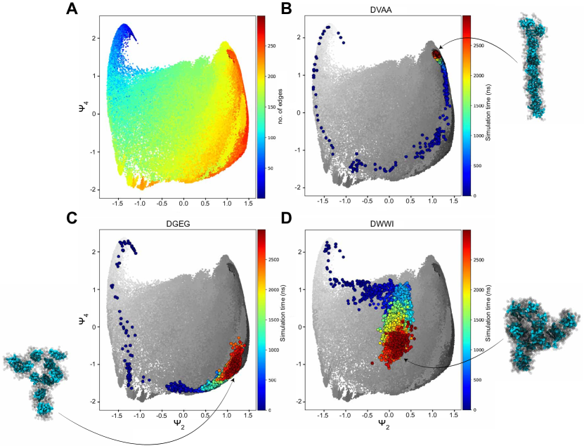
Figure 9: Diffusion map embeddings into $\psi_{2}-\psi_{4}$ of the $N$ = 186 DXXX-OPV3-XXXD molecular simulation trajectories. (a) Composite embedding of all 558,000 simulation snapshots. Each point represents a snapshot from one of the simulation trajectories and points are colored by the total number of edges in the corresponding molecular interaction graph (Section 2.2.1). Temporal assembly courses of selected molecules over the 2D manifold where points are colored by simulation time: (b) DVAA-OPV3-AAVD (good assembler: $\overline{\kappa}$ = 5.85 $\pm$ 0.03, rank = 4/186), (c) DGEG-OPV3-GEGD (intermediate assembler: $\overline{\kappa}$ = 5.02 $\pm$ 0.02, rank = 89/186), (d) DWWI-OPV3-IWWD (poor assembler: $\overline{\kappa}$ = 3.74 $\pm$ 0.01, rank = 175/186).

3.3 Unsupervised spectral clustering into assembly classes

The diffusion map embedding of the assembly trajectories presents a means to identify groups of molecules with similar assembly behaviors and extract design precepts to promote good assembly behavior. We map each of the $N$ = 186 DXXX-OPV3-XXXD molecules in the diffusion map embedding to a single 3D point by averaging over the locations of the final 50 ns of simulation data in the space of the top three nontrivial diffusion map eigenvectors $\{\psi_{i}\}_{i=2}^{4}$. We then perform agglomerative hierarchical clustering using Ward’s method ¹⁰⁴. We cut the resulting dendrogram to partition in the molecules into three clusters (Fig. S2), and illustrate the clustering of the $N$ = 186 molecules within the $\psi_{2}-\psi_{4}$ diffusion map embedding in Fig. 10. The three clusters reveal a natural categorization into good, intermediate, and poor assemblers: (i) the green cluster of points in the top-right of the embedding comprises the good assemblers that form pseudo-1D linear stacks, (ii) the red cluster located in the bottom-right of the manifold contains intermediate assemblers that form loosely connected small linear aggregates, and (iii) the orange cluster located in the bulk of the manifold that forms disordered and disconnected clusters with poor $\pi$-core stacking. We then propagated the cluster labels defined over these $N$ = 186 molecules to the remaining (1,331 - 186) = 1,145 molecules by performing a nearest-neighbor assignation based on distances within the VAE latent space in the terminal round of active learning (Section 2.2.2). A listing of the cluster assignations of each of the 1,331 molecules is provided in Table S3.

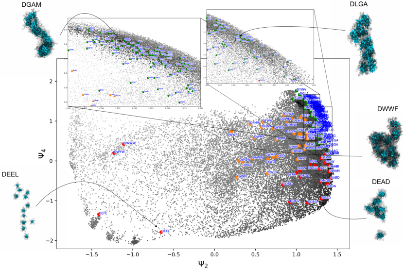
Figure 10: Spectral clustering of the N=186 sampled molecules into four clusters which are projected into the top three non-trivial diffusion map eigenvectors $\{\psi_{i}\}_{i=2}^{4}$. Points are clustered based on agglomerative hierarchical clustering and cutting the resulting dendrogram at the level of three clusters. Grey points represent instantaneous snapshots harvested from all molecular simulations projected into the $\psi_{2}$-$\psi_{4}$ plane. Colored points represent the average coordinates over the terminal 50 ns of simulation for each of the $N$ = 186 molecules. Points are color coded by cluster: green (good assemblers), red (intermediate assemblers), and orange (poor assemblers)

Our classification of the 1,331 molecules allows us to perform a statistical analysis of the enrichment or depletion of amino acid residues in good assemblers relative to intermediate or poor assemblers at each of the the three X_i positions in the DX₁X₂X₃-OPV3-X₃X₂X₁D sequence (Fig. 11). A fuller analysis would account for the complete tripeptide sequence to consider the effects of interactions with the other amino acids, but this simpler one-body analysis is both interpretable and illuminating. Drawing a significance cutoff at 1.5$\times$ enrichment or depletion (p-value = 5$\times$$10^{-21}$, one-tailed Fisher’s exact test), within good assemblers at the X₁ position we observe significant enrichment in $\{A,G,I,L,V\}$ residues and depletion in $\{F,W\}$. At X₂, we observe an enrichment in $\{G,I,L\}$ and impoverishment in $\{F,V,W\}$. Finally, X₃ is enriched in $\{G,I,L,V\}$ and impoverished in $\{W,Y\}$.

First considering the depleted amino acids, the largest hydrophobic residue W is disfavored in good assemblers at all positions. This can be understood as these bulky aromatic side chains possessing favorable $\pi$-stacking interactions with the $\pi$-cores, thereby disrupting $\pi$-core–$\pi$-core stacking. The W residue is most strongly disfavored in the core-adjacent X₃ position, where its bulk and proximity to the core can most effectively disrupt good co-facial core stacking. These observations are consistent with the experimental results in Ref. ²² where smaller UV-vis spectral shifts were observed upon assembly for molecules containing aromatic residues. Of the remaining two aromatic amino acids, F is similarly disfavored, albeit not to the same degree, but the picture for Y is surprisingly nuanced. Y is moderately disfavored at X₁ and strongly disfavored at X₃, but at X₂ it is neither favored nor disfavored. The latter observation was unanticipated, and we currently lack an understanding for why this should be so. This analysis illuminates how location within the tripeptide acts in concert with the inherent physicochemical attributes of an amino acid to modulate its effect.

In regards to the enriched amino acids, the smaller hydrophobic residues G, I, and L are strongly favored at all positions, with I particularly favored in the X₃ position. This preference can be understood as the smaller aliphatic residues enabling closer packing between the peptide wings compared to their bulkier counterparts and their absence of aromatic character reducing interference in the co-facial stacking of $\pi$-cores. Residue A is moderately favored at X₁ and X₂, but neither favored nor disfavored at X₃. Contrariwise, V is moderately to strongly favored at X₁ and X₃, but moderately disfavored at X₂.

Finally, there is no strong preferences for residues D, E, and M at any of the three positions, with the exception of a moderate favorability for M at position X₃.

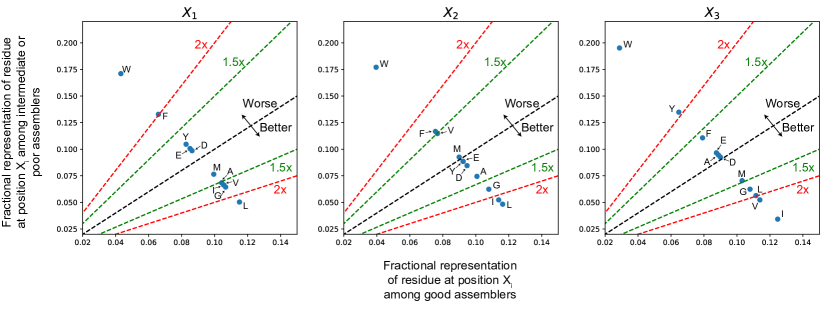
Figure 11: Residue enrichment analysis of each position X_i in DX₁X₂X₃-OPV3-X₃X₂X₁D within molecules classified as good assemblers relative to those classified as intermediate or poor assemblers. Good assemblers are enriched in amino acids residing below the dashed black line and depleted in those residing above it. Dashed green and red lines show boundaries for 1.5$\times$ and 2$\times$ differential enrichment and depletion.

4 Conclusions

The primary goal of this work was to employ molecular simulation to identify members of the DXXX-OPV3-XXXD oligopeptide family exhibiting promising assembly behaviors into pseudo-1D nanoaggregates with good optoelectronic properties, and to discover design precepts for the good assemblers. Trial-and-error exploration of the full chemical space is computationally and experimentally intractable, motivating our use of techniques from optimal experimental design and deep representational learning to efficiently traverse the space of XXX tripeptide sequences and minimize the number of expensive molecular simulations required to identify the top candidates. Employing a combination of coarse-grained molecular simulation, variational autoencoders, Gaussian process regression, and Bayesian optimization, we define an iterative active learning protocol that constructs surrogate models of assembly behavior based on the simulation data collected to date, and uses these models to optimally direct the next round of simulations. The loop is terminated when the surrogate model ceases to improve with additional simulation data and we can reliably predict the top performing molecules. Using this platform we compute a converged rank ordering of the DXXX-OPV3-XXXD oligopeptides in terms of assembly quality after directly simulating only 2.3% of all possible oligopeptide sequences. The calculated ranking list is consistent with existing understanding of what constitutes good and bad sequences for assembly, but also reveals new promising candidate molecules as superior assemblers that have not previously been considered. Our ranked list presents an inexpensive filtration of the complete DXXX-OPV3-XXXD sequence space to direct expensive experimental synthesis and characterization efforts towards the most promising candidate molecules.

A subsequent analysis of the molecular simulation trajectories reveals a low-dimensional manifold within the high-dimensional configurational space over which assembly proceeds. Clustering of the simulation trajectories within this space reveals a natural partitioning of the DXXX-OPV3-XXXD family into good, intermediate, and poor assemblers. Statistical analysis of these classes reveals the good assemblers to be enriched in small and intermediate-sized hydrophobic residues, depleted in large aromatic residues, and that Asp, Glu, and Met do not strongly influence the quality of assembly. The one exception to the latter result is that Met in the X position closest to the $\pi$-core does moderately to strongly favor assembly. These design precepts provide understanding of the rankings established by the active learning protocol.

In sum, this work offers a comprehensive investigation of the assembly landscape of the DXXX-OPV3-XXXD family of $\pi$-conjugated peptides using Bayesian optimal experimental design to guide expensive coarse-grained molecular simulations over microsecond time scales. Our calculations efficiently furnish a rank ordering of the DXXX-OPV3-XXXD and identify a small number of top-performing candidates. While these predictions are only as good as the accuracy of the (coarse-grained) molecular model, they are consistent with existing physicochemical understanding, and can be viewed as a coarse computational filtration of the complete sequence space that can guide subsequent computation and experiment towards the most promising candidates. Ongoing experimental work will attempt to synthesize and test the optoelectronic properties of the candidates in this work, while future computational studies will generalize the approach to D(X)_n-$\Pi$-(X)_nD molecules by extending the considered chemical space to include different $\Pi$ cores, such as perylenediimide (PDI) or oligothiophene (OT), and varying the length of the peptides. Our platform is also generically extensible to the design of other peptide and peptide-like systems, including antimicrobial peptides, cell-penetrating peptides, intrinsically disordered proteins, and peptoids, where the efficient traversal of chemical space, identification of small numbers of top-performing candidates, and exposure of comprehensible design precepts are prioritized.

Data Availability

The coarse-grained molecular simulation trajectories of the self-assembly of the 186 DXXX-OPV3-XXXD molecules conducted in this work are hosted for free public download at the Materials Data Facility ¹⁰⁵, a project affiliated with the NIST Center for Hierarchical Materials Design ^{106, 107} at http://dx.doi.org/10.18126/xqiz-hzc2. Python 3 Jupyter notebooks implementing our active search procedures are available on GitHub at https://github.com/KirillShmilovich/ActiveLearningCG.

TOC Graphic

Figure 12: *

References

- Pinotsi et al. 2016 Pinotsi, D.; Grisanti, L.; Mahou, P.; Gebauer, R.; Kaminski, C. F.; Hassanali, A.; Kaminski Schierle, G. S. Proton transfer and structure-specific fluorescence in hydrogen bond-rich protein structures. Journal of the American Chemical Society 2016, 138, 3046–3057
- Guo et al. 2013 Guo, X.; Baumgarten, M.; Müllen, K. Designing -conjugated polymers for organic electronics. Progress in Polymer Science 2013, 38, 1832–1908
- Kim and Parquette 2012 Kim, S. H.; Parquette, J. R. A model for the controlled assembly of semiconductor peptides. Nanoscale 2012, 4, 6940–6947
- Mitschke and Bäuerle 2000 Mitschke, U.; Bäuerle, P. The electroluminescence of organic materials. Journal of Materials Chemistry 2000, 10, 1471–1507
- Roncali 1992 Roncali, J. Conjugated poly (thiophenes): synthesis, functionalization, and applications. Chemical Reviews 1992, 92, 711–738
- Fichou and Ziegler 1999 Fichou, D.; Ziegler, C. Structure and Properties of Oligothiophenes in the Solid State: Single crystals and thin films; Wiley-VCH: Weinheim, 1999
- Bian et al. 2012 Bian, L.; Zhu, E.; Tang, J.; Tang, W.; Zhang, F. Recent progress in the design of narrow bandgap conjugated polymers for high-efficiency organic solar cells. Progress in Polymer Science 2012, 37, 1292–1331
- Guo et al. 2013 Guo, X.; Baumgarten, M.; Müllen, K. Designing -conjugated polymers for organic electronics. Progress in Polymer Science 2013, 38, 1832–1908
- Newman et al. 2004 Newman, C. R.; Frisbie, C. D.; da Silva Filho, D. A.; Brédas, J.-L.; Ewbank, P. C.; Mann, K. R. Introduction to organic thin film transistors and design of n-channel organic semiconductors. Chemistry of Materials 2004, 16, 4436–4451
- Marder and Lee 2008 Marder, S. R.; Lee, K.-S. Photoresponsive Polymers II; Springer, 2008; Vol. 214
- Beaujuge and Reynolds 2010 Beaujuge, P. M.; Reynolds, J. R. Color control in -conjugated organic polymers for use in electrochromic devices. Chemical Reviews 2010, 110, 268–320
- Marty et al. 2013 Marty, R.; Szilluweit, R.; Sánchez-Ferrer, A.; Bolisetty, S.; Adamcik, J.; Mezzenga, R.; Spitzner, E.-C.; Feifer, M.; Steinmann, S. N.; Corminboeuf, C. et al. Hierarchically structured microfibers of “single stack” perylene bisimide and quaterthiophene nanowires. ACS Nano 2013, 7, 8498–8508
- Löwik et al. 2010 Löwik, D. W. P. M.; Leunissen, E. H. P.; van den Heuvel, M.; Hansen, M. B.; van Hest, J. C. M. Stimulus responsive peptide based materials. Chemical Society Reviews 2010, 39, 3394
- Ulijn and Smith 2008 Ulijn, R. V.; Smith, A. M. Designing peptide based nanomaterials. Chemical Society Reviews 2008, 37, 664
- Marciel et al. 2013 Marciel, A. B.; Tanyeri, M.; Wall, B. D.; Tovar, J. D.; Schroeder, C. M.; Wilson, W. L. Fluidic-directed assembly of aligned oligopeptides with -conjugated cores. Advanced Materials 2013, 25, 6398–6404
- Webber et al. 2016 Webber, M. J.; Appel, E. A.; Meijer, E. W.; Langer, R. Supramolecular biomaterials. Nature Materials 2016, 15, 13–26
- Mansbach and Ferguson 2017 Mansbach, R. A.; Ferguson, A. L. Control of the hierarchical assembly of -conjugated optoelectronic peptides by pH and flow. Organic and Biomolecular Chemistry 2017, 15, 5484–5502
- Schenning and Meijer 2005 Schenning, A. P. H. J.; Meijer, E. W. Supramolecular electronics; nanowires from self-assembled -conjugated systems. Chemical Communications 2005, 3245–3258
- Mba et al. 2011 Mba, M.; Moretto, A.; Armelao, L.; Crisma, M.; Toniolo, C.; Maggini, M. Synthesis and self-assembly of oligo(p-phenylenevinylene) peptide conjugates in water. Chemistry - A European Journal 2011, 17, 2044–2047
- Gallaher et al. 2012 Gallaher, J. K.; Aitken, E. J.; Keyzers, R. A.; Hodgkiss, J. M. Controlled aggregation of peptide-substituted perylene-bisimides. Chemical Communications 2012, 48, 7961
- Facchetti 2011 Facchetti, A. -conjugated polymers for organic electronics and photovoltaic cell applications. Chemistry of Materials 2011, 23, 733–758
- Wall et al. 2014 Wall, B. D.; Zacca, A. E.; Sanders, A. M.; Wilson, W. L.; Ferguson, A. L.; Tovar, J. D. Supramolecular Polymorphism: Tunable electronic interactions within -conjugated peptide nanostructures dictated by primary amino acid sequence. Langmuir 2014, 30, 5946–5956
- Beaujuge and Reynolds 2010 Beaujuge, P. M.; Reynolds, J. R. Color control in -conjugated organic polymers for use in electrochromic devices. Chemical Reviews 2010, 110, 268–320
- Ardoña and Tovar 2015 Ardoña, H. A. M.; Tovar, J. D. Energy transfer within responsive pi-conjugated coassembled peptide-based nanostructures in aqueous environments. Chemical Science 2015, 6, 1474–1484
- Thurston et al. 2016 Thurston, B. A.; Tovar, J. D.; Ferguson, A. L. Thermodynamics, morphology, and kinetics of early-stage self-assembly of -conjugated oligopeptides. Molecular Simulation 2016, 42, 955–975
- Sanders et al. 2017 Sanders, A. M.; Kale, T. S.; Katz, H. E.; Tovar, J. D. Solid-phase synthesis of self-assembling multivalent -conjugated peptides. ACS Omega 2017, 2, 409–419
- Valverde et al. 2018 Valverde, L. R.; Thurston, B. A.; Ferguson, A. L.; Wilson, W. L. Evidence for prenucleated fibrilogenesis of acid-mediated self-assembling oligopeptides via molecular simulation and fluorescence correlation spectroscopy. Langmuir 2018, 34, 7346–7354
- Thurston et al. 2019 Thurston, B.; Shapera, E.; Tovar, J. D.; Schleife, A.; Ferguson, A. L. Revealing the sequence-structure-electronic property relation of self-assembling -conjugated oligopeptides by molecular and quantum mechanical modeling. Langmuir 2019, 35, 15221–15231
- Mansbach and Ferguson 2017 Mansbach, R. A.; Ferguson, A. L. Coarse-grained molecular simulation of the hierarchical self-assembly of -conjugated optoelectronic peptides. Journal of Physical Chemistry B 2017, 121, 1684–1706
- Wall and Tovar 2012 Wall, B. D.; Tovar, J. D. Synthesis and characterization of -conjugated peptide-based supramolecular materials. Pure and Applied Chemistry 2012, 84, 1039–1045
- Thurston and Ferguson 2018 Thurston, B. A.; Ferguson, A. L. Machine learning and molecular design of self-assembling -conjugated oligopeptides. Molecular Simulation 2018, 44, 930–945
- Wall et al. 2011 Wall, B. D.; Diegelmann, S. R.; Zhang, S.; Dawidczyk, T. J.; Wilson, W. L.; Katz, H. E.; Mao, H.-Q.; Tovar, J. D. Aligned macroscopic domains of optoelectronic nanostructures prepared via shear-flow assembly of peptide hydrogels. Advanced Materials 2011, 23, 5009–5014
- Panda et al. 2018 Panda, S. S.; Katz, H. E.; Tovar, J. D. Solid-state electrical applications of protein and peptide based nanomaterials. Chemical Society Reviews 2018, 47, 3640–3658
- Kumar et al. 2011 Kumar, R. J.; MacDonald, J. M.; Singh, T. B.; Waddington, L. J.; Holmes, A. B. Hierarchical self-assembly of semiconductor functionalized peptide -helices and optoelectronic properties. Journal of the American Chemical Society 2011, 133, 8564–8573
- Panda et al. 2019 Panda, S. S.; Shmilovich, K.; Ferguson, A. L.; Tovar, J. D. Controlling supramolecular chirality in peptide- -peptide networks by variation of the alkyl spacer length. Langmuir 2019, 35, 14060–14073
- Marrink et al. 2007 Marrink, S. J.; Risselada, H. J.; Yefimov, S.; Tieleman, D. P.; De Vries, A. H. The MARTINI force field: coarse grained model for biomolecular simulations. The Journal of Physical Chemistry B 2007, 111, 7812–7824
- Monticelli et al. 2008 Monticelli, L.; Kandasamy, S. K.; Periole, X.; Larson, R. G.; Tieleman, D. P.; Marrink, S.-J. The MARTINI coarse-grained force field: extension to proteins. Journal of Chemical Theory and Computation 2008, 4, 819–834
- de Jong et al. 2013 de Jong, D. H.; Singh, G.; Bennett, W. F. D.; Arnarez, C.; Wassenaar, T. A.; Schäfer, L. V.; Periole, X.; Tieleman, D. P.; Marrink, S. J. Improved parameters for the Martini coarse-grained protein force field. Journal of Chemical Theory and Computation 2013, 9, 687–697
- Mansbach and Ferguson 2018 Mansbach, R. A.; Ferguson, A. L. Patchy particle model of the hierarchical self-assembly of -conjugated optoelectronic peptides. The Journal of Physical Chemistry B 2018, 122, 10219–10236
- Kim et al. 2019 Kim, C.; Chandrasekaran, A.; Jha, A.; Ramprasad, R. Active-learning and materials design: The example of high glass transition temperature polymers. MRS Communications 2019, 9, 860–866
- Ling et al. 2017 Ling, J.; Hutchinson, M.; Antono, E.; Paradiso, S.; Meredig, B. High-dimensional materials and process optimization using data-driven experimental design with well-calibrated uncertainty estimates. Integrating Materials and Manufacturing Innovation 2017, 6, 207–217
- Barrett and White 2019 Barrett, R.; White, A. D. Iterative peptide modeling with active learning and meta-learning. arXiv preprint arXiv:1911.09103 2019,
- Gómez-Bombarelli et al. 2018 Gómez-Bombarelli, R.; Wei, J. N.; Duvenaud, D.; Hernández-Lobato, J. M.; Sánchez-Lengeling, B.; Sheberla, D.; Aguilera-Iparraguirre, J.; Hirzel, T. D.; Adams, R. P.; Aspuru-Guzik, A. Automatic chemical design using a data-driven continuous representation of molecules. ACS Central Science 2018, 4, 268–276
- Bickerton et al. 2012 Bickerton, G. R.; Paolini, G. V.; Besnard, J.; Muresan, S.; Hopkins, A. L. Quantifying the chemical beauty of drugs. Nature Chemistry 2012, 4, 90–98
- Xue et al. 2016 Xue, D.; Balachandran, P. V.; Hogden, J.; Theiler, J.; Xue, D.; Lookman, T. Accelerated search for materials with targeted properties by adaptive design. Nature Communications 2016, 7, 1–9
- Yuan et al. 2018 Yuan, R.; Liu, Z.; Balachandran, P. V.; Xue, D.; Zhou, Y.; Ding, X.; Sun, J.; Xue, D.; Lookman, T. Accelerated discovery of large electrostrains in BaTiO3-based piezoelectrics using active learning. Advanced Materials 2018, 30, 1702884
- Gautieri et al. 2010 Gautieri, A.; Russo, A.; Vesentini, S.; Redaelli, A.; Buehler, M. J. Coarse-grained model of collagen molecules using an extended MARTINI force field. Journal of Chemical Theory and Computation 2010, 6, 1210–1218
- Pannuzzo et al. 2014 Pannuzzo, M.; De Jong, D. H.; Raudino, A.; Marrink, S. J. Simulation of polyethylene glycol and calcium-mediated membrane fusion. The Journal of Chemical Physics 2014, 140, 124905
- López et al. 2013 López, C. A.; De Vries, A. H.; Marrink, S. J. Computational microscopy of cyclodextrin mediated cholesterol extraction from lipid model membranes. Scientific Reports 2013, 3, 2071
- Guo et al. 2012 Guo, C.; Luo, Y.; Zhou, R.; Wei, G. Probing the self-assembly mechanism of diphenylalanine-based peptide nanovesicles and nanotubes. ACS Nano 2012, 6, 3907–3918
- Seo et al. 2012 Seo, M.; Rauscher, S.; Pomès, R.; Tieleman, D. P. Improving internal peptide dynamics in the coarse-grained MARTINI model: toward large-scale simulations of amyloid-and elastin-like peptides. Journal of Chemical Theory and Computation 2012, 8, 1774–1785
- Abraham et al. 2015 Abraham, M. J.; Murtola, T.; Schulz, R.; Páll, S.; Smith, J. C.; Hess, B.; Lindahl, E. GROMACS: High performance molecular simulations through multi-level parallelism from laptops to supercomputers. SoftwareX 2015, 1, 19–25
- Bussi et al. 2007 Bussi, G.; Donadio, D.; Parrinello, M. Canonical sampling through velocity rescaling. The Journal of Chemical Physics 2007, 126, 014101
- Parrinello and Rahman 1981 Parrinello, M.; Rahman, A. Polymorphic transitions in single crystals: A new molecular dynamics method. Journal of Applied Physics 1981, 52, 7182–7190
- Hockney and Eastwood 1988 Hockney, R. W.; Eastwood, J. W. Computer Simulation Ssing Particles; CRC Press, 1988
- Hess et al. 1997 Hess, B.; Bekker, H.; Berendsen, H. J. C.; Fraaije, J. G. E. M. LINCS: A linear constraint solver for molecular simulations. Journal of Computational Chemistry 1997, 18, 1463–1472
- Pedregosa et al. 2011 Pedregosa, F.; Varoquaux, G.; Gramfort, A.; Michel, V.; Thirion, B.; Grisel, O.; Blondel, M.; Prettenhofer, P.; Weiss, R.; Dubourg, V. et al. Scikit-learn: machine learning in Python. Journal of Machine Learning Research 2011, 12, 2825–2830
- Oliphant 2015 Oliphant, T. E. Guide to NumPy, 2nd ed.; CreateSpace Independent Publishing Platform, 2015
- Chollet 2015 Chollet, F. keras. https://github.com/fchollet/keras, 2015
- Hočevar and Demšar 2014 Hočevar, T.; Demšar, J. A combinatorial approach to graphlet counting. Bioinformatics 2014, 30, 559–565
- Wang and Ferguson 2016 Wang, J.; Ferguson, A. L. Mesoscale simulation of asphaltene aggregation. The Journal of Physical Chemistry B 2016, 120, 8016–8035
- Humphrey et al. 1996 Humphrey, W.; Dalke, A.; Schulten, K. VMD: visual molecular dynamics. Journal of Molecular Graphics 1996, 14, 33–8
- Hagberg et al. 2008 Hagberg, A.; Swart, P.; S Chult, D. Exploring network structure, dynamics, and function using NetworkX; Technical Report, Los Alamos National Lab.(LANL), Los Alamos, NM, 2008
- Henikoff and Henikoff 1992 Henikoff, S.; Henikoff, J. G. Amino acid substitution matrices from protein blocks. Proceedings of the National Academy of Sciences 1992, 89, 10915–10919
- Kingma and Welling 2013 Kingma, D. P.; Welling, M. Auto-encoding variational Bayes. arXiv preprint arXiv:1312.6114 2013,
- Calandra et al. 2016 Calandra, R.; Peters, J.; Rasmussen, C. E.; Deisenroth, M. P. Manifold Gaussian processes for regression. 2016 International Joint Conference on Neural Networks (IJCNN). 2016; pp 3338–3345
- Doersch 2016 Doersch, C. Tutorial on variational autoencoders. arXiv preprint arXiv:1606.05908 2016,
- Kingma and Ba 2014 Kingma, D. P.; Ba, J. Adam: A method for stochastic optimization. arXiv preprint arXiv:1412.6980 2014,
- Brochu et al. 2010 Brochu, E.; Cora, V. M.; De Freitas, N. A tutorial on Bayesian optimization of expensive cost functions, with application to active user modeling and hierarchical reinforcement learning. arXiv preprint arXiv:1012.2599 2010,
- Sivia and Skilling 2006 Sivia, D.; Skilling, J. Data Analysis: A Bayesian Tutorial; Oxford University Press, 2006
- Ebden 2015 Ebden, M. Gaussian processes: A quick introduction. arXiv preprint arXiv:1505.02965 2015,
- Rasmussen and Williams 2005 Rasmussen, C. E.; Williams, C. K. I. Gaussian Processes for Machine Learning (Adaptive Computation and Machine Learning); The MIT Press, 2005
- Mohammadi et al. 2016 Mohammadi, H.; Riche, R. L.; Durrande, N.; Touboul, E.; Bay, X. An analytic comparison of regularization methods for Gaussian processes. arXiv preprint arXiv:1602.00853 2016,
- Močkus 1975 Močkus, J. On Bayesian methods for seeking the extremum. Optimization techniques IFIP technical conference. 1975; pp 400–404
- Jones et al. 1998 Jones, D. R.; Schonlau, M.; Welch, W. J. Efficient global optimization of expensive black-box functions. Journal of Global Optimization 1998, 13, 455–492
- Lizotte 2008 Lizotte, D. J. Practical Bayesian optimization. Ph.D. thesis, 2008
- Lorenz et al. 2016 Lorenz, R.; Monti, R. P.; Violante, I. R.; Anagnostopoulos, C.; Faisal, A. A.; Montana, G.; Leech, R. The Automatic Neuroscientist: A framework for optimizing experimental design with closed-loop real-time fMRI. NeuroImage 2016, 129, 320–334
- Schohn and Cohn 2000 Schohn, G.; Cohn, D. Less is more: Active learning with support vector machines. ICML. 2000; p 6
- Vlachos 2008 Vlachos, A. A stopping criterion for active learning. Computer Speech & Language 2008, 22, 295–312
- Zhu et al. 2008 Zhu, J.; Wang, H.; Hovy, E. Multi-criteria-based strategy to stop active learning for data annotation. Proceedings of the 22nd International Conference on Computational Linguistics-Volume 1. 2008; pp 1129–1136
- Bloodgood and Vijay-Shanker 2014 Bloodgood, M.; Vijay-Shanker, K. A method for stopping active learning based on stabilizing predictions and the need for user-adjustable stopping. arXiv preprint arXiv:1409.5165 2014,
- Bloodgood and Grothendieck 2015 Bloodgood, M.; Grothendieck, J. Analysis of stopping active learning based on stabilizing predictions. arXiv preprint arXiv:1504.06329 2015,
- Beatty et al. 2019 Beatty, G.; Kochis, E.; Bloodgood, M. The use of unlabeled data versus labeled data for stopping active learning for text classification. 2019 IEEE 13th International Conference on Semantic Computing (ICSC). 2019; pp 287–294
- Bhattacharyya 1946 Bhattacharyya, A. On a measure of divergence between two multinomial populations. Sankhyā: The Indian Journal of Statistics 1946, 401–406
- Bloodgood and Vijay-Shanker 2014 Bloodgood, M.; Vijay-Shanker, K. Taking into account the differences between actively and passively acquired data: The case of active learning with support vector machines for imbalanced datasets. arXiv preprint arXiv:1409.4835 2014,
- Long and Ferguson 2018 Long, A. W.; Ferguson, A. L. Rational design of patchy colloids via landscape engineering. Molecular Systems Design & Engineering 2018, 3, 49–65
- Wang and Ferguson 2018 Wang, J.; Ferguson, A. L. Nonlinear machine learning in simulations of soft and biological materials. Molecular Simulation 2018, 44, 1090–1107
- Ma and Ferguson 2019 Ma, Y.; Ferguson, A. L. Inverse design of self-assembling colloidal crystals with omnidirectional photonic bandgaps. Soft Matter 2019, 15, 8808–8826
- Przulj 2007 Przulj, N. Biological network comparison using graphlet degree distribution. Bioinformatics 2007, 23, e177–e183
- Aparício et al. 2017 Aparício, D.; Ribeiro, P.; Silva, F. Temporal network comparison using graphlet-orbit transitions. arXiv preprint arXiv:1707.04572 2017,
- Shervashidze and Borgwardt 2009 Shervashidze, N.; Borgwardt, K. Fast subtree kernels on graphs. Advances in Neural Information Processing Systems. 2009; pp 1660–1668
- Kashima et al. 2003 Kashima, H.; Tsuda, K.; Inokuchi, A. Marginalized kernels between labeled graphs. Proceedings of the 20th international conference on machine learning (ICML-03). 2003; pp 321–328
- Bonner et al. August 2016 Bonner, S.; Brennan, J.; Theodoropoulos, G.; Kureshi, I.; McGough, A. Efficient comparison of massive graphs through the use of "graph fingerprints". Twelfth Workshop on Mining and Learning with Graphs (MLG) ’16 SanFrancisco, California USA. August 2016
- Reinhart and Panagiotopoulos 2018 Reinhart, W. F.; Panagiotopoulos, A. Z. Automated crystal characterization with a fast neighborhood graph analysis method. Soft Matter 2018, 14, 6083–6089
- Coifman and Lafon 2006 Coifman, R. R.; Lafon, S. Diffusion maps. Applied and Computational Harmonic Analysis 2006, 21, 5–30
- Wang et al. 2017 Wang, J.; Gayatri, M. A.; Ferguson, A. L. Mesoscale simulation and machine learning of asphaltene aggregation phase behavior and molecular assembly landscapes. The Journal of Physical Chemistry B 2017, 121, 4923–4944
- Nadler et al. 2006 Nadler, B.; Lafon, S.; Kevrekidis, I.; Coifman, R. R. Diffusion maps, spectral clustering and eigenfunctions of Fokker-Planck operators. Advances in Neural Information Processing Systems. 2006; pp 955–962
- Wang and Ferguson 2018 Wang, J.; Ferguson, A. L. A study of the morphology, dynamics, and folding pathways of ring polymers with supramolecular topological constraints using molecular simulation and nonlinear manifold learning. Macromolecules 2018, 51, 598–616
- Ardona et al. 2015 Ardona, H. A. M.; Besar, K.; Togninalli, M.; Katz, H. E.; Tovar, J. D. Sequence-dependent mechanical, photophysical and electrical properties of pi-conjugated peptide hydrogelators. Journal of Materials Chemistry C 2015, 3, 6505–6514
- Vadehra et al. 2010 Vadehra, G. S.; Wall, B. D.; Diegelmann, S. R.; Tovar, J. D. On-resin dimerization incorporates a diverse array of -conjugated functionality within aqueous self-assembling peptide backbones. Chemical Communications 2010, 46, 3947–3949
- Besar 2016 Besar, K. Organic semiconductor devices for chemical sensing and bio interfaces. Ph.D. thesis, Johns Hopkins University, 2016
- Ferguson et al. 2010 Ferguson, A. L.; Panagiotopoulos, A. Z.; Debenedetti, P. G.; Kevrekidis, I. G. Systematic determination of order parameters for chain dynamics using diffusion maps. Proceedings of the National Academy of Sciences 2010, 107, 13597–13602
- Rubinstein and Colby 2003 Rubinstein, M.; Colby, R. H. Polymer Physics; Oxford University Press, 2003
- Ward 1963 Ward, J. H. Hierarchical Grouping to Optimize an Objective Function. Journal of the American Statistical Association 1963, 58, 236–244
- Shmilovich et al. 2019 Shmilovich, K.; Mansbach, R. A.; Ferguson, A. L. Dataset for discovery of self-assembling -conjugated peptides by active learning-directed coarse-grained molecular simulation. Materials Data Facility 2019, DOI: 10.18126/xqiz–hzc2
- Blaiszik et al. 2016 Blaiszik, B.; Chard, K.; Pruyne, J.; Ananthakrishnan, R.; Tuecke, S.; Foster, I. The Materials Data Facility: Data services to advance materials science research. JOM 2016, 68, 2045–2052
- Blaiszik et al. 2019 Blaiszik, B.; Ward, L.; Schwarting, M.; Gaff, J.; Chard, R.; Pike, D.; Chard, K.; Foster, I. A data ecosystem to support machine learning in materials science. MRS Communications 2019, 9, 1125–1133