Pixel-wise Conditioned Generative Adversarial Networks for Image Synthesis and Completion
Abstract
Generative Adversarial Networks (GANs) have proven successful for unsupervised image generation. Several works have extended GANs to image inpainting by conditioning the generation with parts of the image to be reconstructed. Despite their success, these methods have limitations in settings where only a small subset of the image pixels is known beforehand. In this paper we investigate the effectiveness of conditioning GANs when very few pixel values are provided. We propose a modelling framework which results in adding an explicit cost term to the GAN objective function to enforce pixel-wise conditioning. We investigate the influence of this regularization term on the quality of the generated images and the fulfillment of the given pixel constraints. Using the recent PacGAN technique, we ensure that we keep diversity in the generated samples. Conducted experiments on FashionMNIST show that the regularization term effectively controls the trade-off between quality of the generated images and the conditioning. Experimental evaluation on the CIFAR-10 and CelebA datasets evidences that our method achieves accurate results both visually and quantitatively in term of Fréchet Inception Distance, while still enforcing the pixel conditioning. We also evaluate our method on a texture image generation task using fully-convolutional networks. As a final contribution, we apply the method to a classical geological simulation application.
keywords:
deep generative models, generative adversarial networks, conditional GAN1 Introduction
Generative modelling is the process of modelling a distribution in a high-dimension space in a way that allows sampling in it. Generative Adversarial Networks (GANs) [1] have been the state of the art in unsupervised image generation for the past few years, being able to produce realistic images with high resolution [2] without explicitly modelling the samples distribution. GANs learn a mapping function of vectors drawn from a low dimensional latent distribution (usually normal or uniform) to high dimensional ground truth images issued from an unknown and complex distribution. By using a discrimination function that distinguishes real images from generated ones, GANs setups a min max game able to approximate a Jensen-Shannon divergence between the distributions of the real samples and the generated ones.
Among extensions of GANs, Conditional GAN (CGAN) [3] attempts to condition the generation procedure on some supplementary information (such as the label of the image ) by providing to the generation and discrimination functions. CGAN enables a variety of conditioned generation, such as class-conditioned image generation [3], image-to-image translation [4, 5], or image inpainting [6]. On the other side, Ambient GAN [7] aims at training an unconditional generative model using only noisy or incomplete samples . Relevant application domain is high-resolution imaging (CT scan, fMRI) where image sensing may be costly. Ambient GAN attempts to produce unaltered images which distribution matches the true one without accessing to the original images . For the sake, Ambient GAN considers lossy measurements such as blurred images, images with removed patch or removed pixels at random (up to 95%). Following this setup, Pajot et al.[8] extend the learning strategy to enable the reconstruction instead of the generation of realistic images from similarly altered samples.
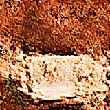
In the spirit of Ambient GAN, we consider in this paper an extreme setting of image generation when only a few pixels, less than a percent of the image size, are known and are randomly scattered across the image (see Fig.1(c)). We refer to these conditioning pixels as a constraint map . To reconstruct the missing information, we design a generative adversarial model able to generate high quality images coherent with given pixel values by leveraging on a training set of similar, but not paired images. The model we propose aims to match the distribution of the real images conditioned on a highly scarce constraint map, drawing connections with Ambient GAN while, in the same manner as CGAN, still allowing the generation of diverse samples following the underlying conditional distribution.
To make the generated images honoring the prescribed pixel values, we use a reconstruction loss measuring how close real constrained pixels are to their generated counterparts. We show that minimizing this loss is equivalent to maximizing the log-likelihood of the constraints given the generated image. Thereon we derive an objective function trading-off the adversarial loss of GAN and the reconstruction loss which acts as a regularization term. We analyze the influence of the related hyper-parameter in terms of quality of generated images and the respect of the constraints. Specifically, empirical evaluation on FashionMNIST [9] evidences that the regularization parameter allows for controlling the trade-off between samples quality and constraints fulfillment.
Additionally to show the effectiveness of our approach, we conduct experiments on CIFAR10 [10], CelebA [11] or texture [12] datasets using various deep architectures including fully convolutional network. We also evaluate our method on a classical geological problem which consists of generating 2D geological images of which the spatial patterns are consistent with those found in a conceptual image of a binary fluvial aquifer[13][14]. Empirical findings reveal that the used architectures may lack stochasticity from the generated samples that is the GAN input is often mapped to the same output image irrespective of the variations in latent code [15]. We address this issue by resorting to the recent PacGAN [16] strategy. As a conclusion, our approach performs well both in terms of visual quality and respect of the pixel constraints while keeping diversity among generated samples. Evaluations on CIFAR-10 and CelebA show that the proposed generative model always outperforms the CGAN approach on the respect of the constraints and either come close or outperforms it on the visual quality of the generated samples.
The remainder of the paper is organized as follows. In Section 2, we review the relevant related work focusing first on generative adversarial networks, their conditioned version and then on methods dealing with image generation and reconstruction from highly altered training samples. Section 3 details the overall generative model we propose. In Section 4, we present the experimental protocol and evaluation measures while Section 5 gathers quantitative and qualitative effectiveness of our approach. The last section concludes the paper.
The contributions of the paper are summarized as follows:
-
•
We propose a method for learning to generate images with a few pixel-wise constraints.
-
•
A theoretical justification of the modelling framework is investigated.
-
•
A controllable trade-off between the image quality and the constraints’ fulfillment is highlighted,
-
•
We showcase a lack of diversity in generating high-dimensional images which we solve by using PacGAN[16] technique. Several experiments allow to conclude that the proposed formulation can effectively generate diverse and high visual quality images while satisfying the pixel-wise constraints.
2 Image reconstruction with GAN in related works
The pursued objective of the paper is image generation using generative deep network conditioned on randomly scattered and scarce (less than a percent of the image size) pixel values. This kind of pixel constraints occurs in application domains where an image or signal need to be generated from very sparse measurements.
Before delving into the details, let introduce the notations and previous work related to the problem. We denote by a random variable and its realization. Let be the distribution of over and be its evaluation at . Similarly represents the distribution of conditioned on the random variable .
Given a set of images (see Figure 1(a)) drawn from an unknown distribution and a sparse matrix (Figure 1(c)) as the given constrained pixels, the problem consists in finding a generative model with inputs (a random vector sampled from a known distribution over the space ) and constrained pixel values able to generate an image satisfying the constraints while likely following the distribution (see Figure 3).

Image

Input
Map
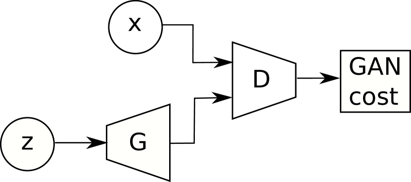
One of the state-of-the-art modelling framework for image generation is the Generative Adversarial Network. The seminal version of GAN [1] learns the generative models in an unsupervised way. It relies on a game between a generation function and a discrimination network , in which learns to produce realistic samples while learns to distinguish real examples from generated ones (Figure 2(a)). Training GANs amounts to find a Nash equilibrium to the following min-max problem,
| (1) |
where is a known distribution, usually normal or uniform, from which the latent input of is drawn, and is the distribution of the real images.
Among several applications, the GANs was adapted to image inpainting task (Figure 1(b)). For instance Yeh et al. [17] propose an inpainting approach which considers a pre-trained generator, and explores its latent space through an optimization procedure to find a latent vector , which induces an image with missing regions filled in by conditioning on the surroundings available information. However, the method requires to solve a full optimization problem at inference stage, which is computationally expensive.
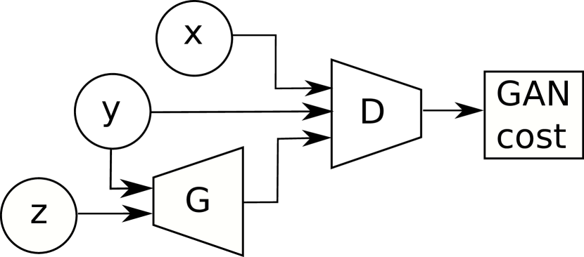
Other approaches (Figure 2) rely on Conditional variant of GAN (CGAN) [3] in which additional information is provided to the generator and the discriminator (see Figure 2(b)). This leads to the following optimization problem adapted to CGAN
| (2) |
Although CGAN was initially designed for class-conditioned image generation by setting as the class label of the image, several types of conditioning information can apply such as a full image for image-to-image translation [4] or partial image as in inpainting [18]. CGAN-based inpainting methods rely on generating a patch that will fill up a structured missing part of the image and achieve impressive results. However they are not well suited to reconstruct very sparse and unstructured signal [19]. Additionally, these approaches learn to reconstruct a single sample instead of a full distribution, implying that there is no sampling process for a given constraint map or highly degraded image.
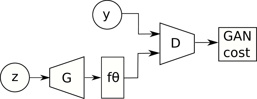
AmbientGAN [7] (Figure 2(c)) trains a generative model capable to yield full images from only lossy measurements. One of the image degradations considered in this approach is the random removal of pixels leading to sparse pixel map . It is simulated with a differentiable function whose parameter indicates the pixels to be removed. The underlying optimization problem solved by AmbientGAN is therefore stated as
| (3) |
Pajot et al. [8] combined the AmbientGAN approach with an additional reconstruction task that consists in reconstructing the from the twice-altered image and ,
| (4) |
The norm term ensures that the generator is able to learn to revert i.e. to revert the alteration process on a given sample. This allows the reconstruction of realistic image only from a given constraint map . However the reconstruction process is deterministic and does not provide a sampling mechanism.
Compressed Sensing with Meta-Learning [20] is an approach that combines the exploration of the latent space to recover images from lossy measurements with the enforcing of the Restricted Isometric Property [21], which states that for two samples ,
where is a small constant. It replaces the adversarial training of the generative model (Eq. 1) by searching, for a given degraded image , a vector such that minimizes the distance between and while still enforcing the RIP. The overall problem induced by this approach can be formulated as:
| (5) |
where contains the three samples . In practice, is computed with gradient descent on by minimizing , and starting from a random . As a benefit, this approach may generate an image from a noisy information but at a high computation burden since it requires to solve an optimization problem (computing ) at inference stage for generating an image.
3 Proposed approach
Let introduce the formal formulation of the addressed problem. Assume is the given set of constrained pixel values. To ease the presentation, let consider as a image with only a few available pixels (less than of ). We will also encode the spatial location of these pixels using a corresponding binary mask . We intend to learn a GAN whose generation network takes as input the constraint map and the sampled latent code and outputs a realistic image that fulfills the prescribed pixel values. Within this setup, the generative model can sample from the unknown distribution of the training images while satisfying unseen pixel-wise constraints at training stage. Formally our proposed GAN can be formulated as
| (6) | |||
where stands for the Hadamard (or point-wise) product and for the mask, a sparse matrix with entries equal to one at constrained pixels location.
As the equality constraint in Problem (6) is difficult to enforce during training, we rather investigate a relaxed version of the problems. Following Pajot et al. [8] we assume that the constraint map is obtained through a noisy measurement process
| (7) |
Here is the masking operator yielding to . Also the constrained pixels are randomly and independently selected. represents an additive i.i.d noise corrupting the pixels. Therefore we can formulate the Maximum A Posteriori (MAP) estimation problem, which, given the constraint map , consists in finding the most probable image following the posterior distribution ,
| (8) | ||||
| (9) |
is the likelihood that the constrained pixels are issued from image while represents the prior probability at . Assuming that the generation network may sample the most probable image complying with the given pixel values , we get the following problem
| (10) |
The first term in Problem (10) measures the likelihood of the constraints given a generated image. Let rewrite Equation (7) as where is the vectorisation operator that consists in stacking the constrained pixels. Therefore, assuming is an i.i.d Gaussian noise with distribution , we achieve the expression of the conditional likelihood
| (11) |
which evaluates the quadratic distance between the conditioning pixels and their predictions by . In other words, using a matrix notation of (7), the likelihood of the constraints given a generated image equivalently writes
| (12) |
represents the squared Frobenius norm of matrix that is the sum of its squared entries.
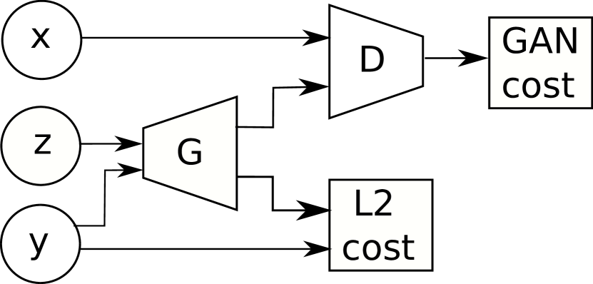
The second term in Problem (10) is the likelihood of the generated image under the true but unknown data distribution . Maximizing this term can be equivalently achieved by minimizing the distance between and the marginal distribution of the generated samples . This amounts to minimizing with respect to , the GAN-like objective function [1]. Putting altogether these elements, we can propose a relaxation of the hard constraint optimization problem (6) (Figure 2(d)) as follows
Remarks:
-
•
The assumption of Gaussian noise measurement leads us to explicitly turn the pixel value constraints into the minimization of the norm between the real enforced pixel values and their generated counterparts (see Figure 2(d)).
-
•
This additional term acts as a regularization over prescribed pixels by the mask . The trade-off between the distribution matching loss and the constraint enforcement is assessed by the regularization parameter .
-
•
It is worth noting that the noise can be of any other distribution, according to the prior information, one may associate to the measurement process. We only require this distribution to admit a closed-form solution for the maximum likelihood estimation for optimization purpose. Typical choices are distributions from the exponential family [22].

Image


Image

Consts.
To solve Problem (3), we use the stochastic gradient descent method. The overall training procedure is detailed in Algorithm 1 and ends up when a maximal number of training epochs is attained.
When implementing this training procedure we experienced, at inference stage, a lack of diversity in the generated samples (see Figure 5) with deeper architectures, most notably the encoder-decoder architectures. This issue manifests itself through the fact that the learned generation network, given a constraint map , outputs almost deterministic image regardless the variations in the input . The issue was also pointed out by Yang et al. [15] as characteristic of CGANs.
To avoid the problem, we exploit the recent PacGAN [16] technique: it consists in passing a set of samples to the discrimination function instead of a single one. PacGAN is intended to tackle the mode collapse problem in GAN training. The underlying principle being that if a set of images are sampled from the same training set, they are very likely to be completely different, whereas if the generator experiences mode collapse, generated images are likely to be similar. In practice, we only give two samples to the discriminator, which is sufficient to overcome the loss of diversity as suggested in [16]. The resulting training procedure is summarized in Algorithm 2.
4 Experiments
We have conducted a series of empirical evaluation to assess the performances of the proposed GAN. Used datasets, evaluation protocol and the tested deep architectures are detailed in this section while Section 5 is devoted to the results presentation.
4.1 Datasets
We tested our approach on several datasets listed hereafter. Detailed information on these datasets are provided in the Appendix A.
-
CIFAR10 [10] consists of 60,000 colour images of 10 different and varied classes. It is deemed less easy than MNIST and FashionMnist
-
CelebA[11] is a large dataset of celebrity portraits labeled by identity and a variety of binary features such as eyeglasses, smiling… We use 100,000 images cropped to a size of , making this dataset appropriate for a high dimension evaluation of our approach in comparison with related work.
-
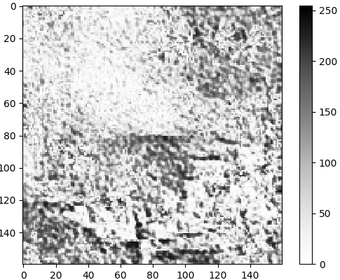
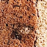
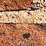
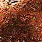
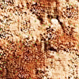
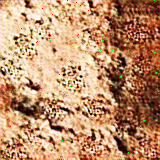
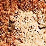
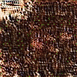
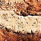
Texture is a custom dataset composed of patches sampled from a large brick wall texture, as recommended in [12]. It is worth noting that this procedure can be reproduced on any texture image of sufficient size. Texture is a testbed of our approach on fully-convolutional networks for constrained texture generation task.
-
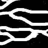
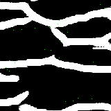
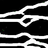
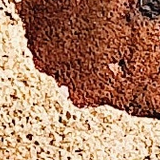
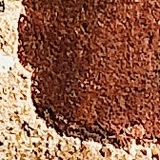
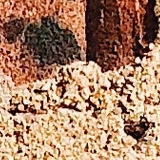
Subsurface is a classical dataset in geological simulation [13] which consists, similarly to the Texture dataset, of 20,000 patches sampled from a model of a subsurface binary domain. These models are assumed to have the same properties as a texture, mainly the property of global ergodicity of the data.
To avoid learning explicit pairing of real images seen by the discrimination function with constraint maps provided to the generative network, we split each dataset into training, validation and test sets, to which we add a set composed of constraint maps that should remain unrelated to the three others. In order to do so, a fifth of each set is used to generate the constrained pixel map by randomly selecting of the pixels from a uniform distribution, composing a set of constraints for each of the train, test and validation sets. The images from which these maps are sampled are then removed from the training, testing and validation sets. For each carried experiment the best model is selected based on some performance measures (see Section 4.3) computed on the validation set, as in the standard of machine learning methodology [24]. Finally, reported results are computed on the test set.
4.2 Network architectures
We use a variety of GAN architectures in order to adapt to the different scales and image sizes of our datasets. The detailed configuration of these architectures are exposed in Appendix B.
For the experiments on the FashionMNIST [9], we use a lightweight network for both the discriminator and the generator similarly to DCGAN [25] due to the small resolution of FashionMnist images.
To experiment on the Texture dataset, we consider a set of fully-convolutional generator architectures based on either dilated convolutions [26], which behave well on texture datasets [27], or encoder-decoder architectures that are commonly used in domain-transfer applications such as CycleGAN [28]. We selected these architectures because they have very large receptive fields without using pooling, which allow the generator to use a large context for each pixel.
We keep the same discriminator across all the experiments with these architectures, the PatchGAN discriminator [4], which is a five-layer fully-convolutional network with a sigmoid activation.
The Up-Dil architecture consists in a set of transposed convolutions (the upscaling part), and a set of dilated convolutional layers [26], while the Up-EncDec has an upscaling part followed by an encoder-decoder section with skip-connections, where the constraints are downscaled, concatenated to the noise, and re-upscaled to the output size.
The UNet [29] architecture is an encoder-decoder where skip-connections are added between the encoder and the decoder. The Res architecture is an encoder-decoder where residual blocks [30] are added after the noise is concatenated to the features. The UNet-Res combines the UNet and the Res architectures by including both residual blocks and skip-connections.
Finally, we will evaluate our approach on the Subsurface dataset using the architecture that yields to the best performances on the Texture dataset.
4.3 Evaluation
We evaluate our approach based on both the satisfaction of the pixel constraints and the visual quality of sampled images. From the assumption of Gaussian measurement noise (as discussed in Section 3), we assess the constraint fulfillment using the following mean square error (MSE)
| (14) |
This metric should be understood as the mean squared error of reconstructing the constrained pixel values.
Visual quality evaluation of an image is not a trivial task [31]. However, Fréchet Inception Distance (FID) [32] and Inception Score [33], have been used to evaluate the performance of generative models. We employ FID since the Inception Score has been shown to be less reliable [34]. The FID consists in computing a distance between the distributions of relevant features extracted from generated and real samples. To extract these features, a pre-trained Inception v3 [35] classifier is used to compute the embeddings of the images at a chosen layer. Assuming these embeddings shall follow a normal distribution, the quality of the generated images is assessed in term of a Wasserstein-2 distance between the distribution of real samples and generated ones. Hence the FID writes
| (15) |
where is the trace operator, (, ) and (, ) are the pairs of mean vector and covariance matrice of embeddings obtained on respectively the real and the generated data. Being a distance between distributions, a small FID corresponds to a good matching of the distributions.
Since the FID requires a pre-trained classifier adapted to the dataset in study, we trained simple convolutional neural networks as classifiers for the FashionMNIST and the CIFAR-10 datasets. For the Texture dataset, since the dataset is not labeled, we resort to a CNN classifier trained on the Describable Textures Dataset (DTD) [36], which is a related application domain.
However, since we do not have labels for the Subsurface dataset, we could not train a classifier for this dataset, thus we cannot compute the FID. To evaluate the quality of the generated samples, we use metrics based on a distance between feature descriptors extracted from real samples and generated ones. Similarly to [27], we rely on a distance between the Histograms of Oriented Gradients (HOG) or Local Binary Patterns (LBP) features computed on generated and real images.
Histograms of Oriented Gradients (HOG) [37] and Local Binary Patterns (LBP) [38] are computed by splitting an image into cells of a given radius and computing on each cell the histograms of the oriented gradients for HOGs and of the light level differences for each pixel to the center of the cell for LBPs. Additionally, we consider the domain-specific metric, the connectivity function [39] which is presented in Appendix C.
Finally, we check by visual inspection if the trained model is able to generate diverse samples, meaning that for a given and for a set of latent codes , the generated samples are visually different.
5 Experimental results
5.1 Quality-fidelity trade-off

We first study the influence of the regularization hyper-parameter on both the quality of the generated samples and the respect of the constraints. We experiment on the FashionMNIST [9] dataset, since such a study requires intensive simulations permitted by the low resolution of FashionMnist images and the used architectures (see Section 4.2).
To overcome classical GANs instability, the networks are trained 10 times and the median values of the best scores on the test set at the best epoch are recorded. The epoch that minimizes:
on the validation set is considered as the best epoch, where , , and are respectively the lowest and highest FIDs and MSEs obtained on the validation set.
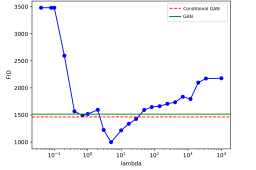
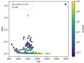
Empirical evidences (highlighted in Figure 4) show that with a good choice of , the regularization term helps the generator to enforce the constraints, leading to smaller MSEs than when using the CGAN () without compromising on the quality of generated images. Also, we can note that using the regularization term even leads to a better image quality compared to GAN and CGAN. The bottom panel in Figure 4 illustrates that the trade-off between image quality and the satisfaction of the constraints can be controlled by appropriately setting the value of . Nevertheless, for small values of (less or equal to ), our GAN model fails to learn meaningful distribution of the training images and only generates uniformly black images. This leads to the plateaus on the MSE and FID plots (top panels in Figure 4).
5.2 Texture generation with fully-convolutional architectures
Fully-convolutional architectures for GANs are widely used, either for domain-transfer applications [28][4] or for texture generation [12]. In order to evaluate the efficiency of our method on relatively high resolution images, we experiment the fully-convolutional networks described in Section 4.2 on a texture generation task using Texture dataset. We investigate the upscaling-dilatation network, the encoder-decoder one and the resnet-like architectures.
Our training algorithm was run for 40 epochs on all reported results. We provide a comparison to CGAN[3] approach by using the selected best architectures. The models are evaluated in terms of best FID (visual quality of sampled images) at each epoch and MSE (conditioning on fixed pixel values). We also compute the FID score of the models at the epochs where the MSE is the lowest. In the other way around, the MSE is reported at epoch when the FID is the lowest. The obtained quantitative results are detailed in Table 1.
For the encoder-decoder models, we can notice that the models using ResNet blocks perform better than just using a UNet generator. A trade-off can also be seen between the FID and MSE for the ResNet models and the UNet-ResNet, which could mean that skip-connections help the generator to fulfill the constraints but at the price of lowered visual quality.
Although the encoder-decoder models perform the best, they tend to lose diversity in the generated samples (see Figure 5), whereas the upscaling-based models have high FID and MSE but naturally preserve diversity in the generated samples.

Changing the discriminator for a PacGAN discriminator with 2 samples in the encoder-decoder based architectures allows to restore diversity, while keeping the same performances as previously or even increasing the performances for the UNetRes (see Table 1).
Table 2 compares our proposed approach to CGAN using fully convolutional networks. It shows that our approach is more able to comply with the pixel constraints while producing realistic images. Indeed, our approach outperforms CGAN (see Table 2) by a large margin on the respect of conditioning pixels (see the achieved MSE metrics by our UNetPAC or UNetResPAC) and gets close FID performance on the generated samples. This finding is in accordance of the obtained results on FashionMnist experiments.
| Model | Best FID | Best MSE | FID at | MSE at | Diversity |
|---|---|---|---|---|---|
| best MSE | best FID | ||||
| Up-Dil | 0.0949 | 0.4137 | 1.0360 | 0.7057 | ✓ |
| Up-EncDec | 0.1509 | 0.7570 | 0.2498 | 0.9809 | ✓ |
| UNet | 0.0442 | 0.1789 | 0.0964 | 0.4559 | ✗ |
| Res | 0.0458 | 0.0474 | 0.0590 | 0.0476 | ✗ |
| UNetRes | 0.0382 | 0.0307 | 0.0499 | 0.0338 | ✗ |
| ResPAC | 0.0350 | 0.0698 | 0.0466 | 0.4896 | ✓ |
| UNetPAC | 0.0672 | 0.0001 | 0.3120 | 0.2171 | ✓ |
| UNetResPAC | 0.0431 | 0.0277 | 0.0447 | 0.0302 | ✓ |
| Model | Best FID | Best MSE | FID at | MSE at |
|---|---|---|---|---|
| best MSE | best FID | |||
| CGAN-ResPAC | 0.0234 | 0.1337 | 0.0340 | 0.2951 |
| CGAN-UNetPAC | 0.0518 | 0.2010 | 0.0705 | 0.4828 |
| CGAN-UNetResPAC | 0.0428 | 0.1060 | 0.0586 | 0.2250 |
| Ours-ResPAC | 0.0350 | 0.0698 | 0.0466 | 0.4896 |
| Ours-UNetPAC | 0.0672 | 0.0001 | 0.3120 | 0.2171 |
| Ours-UNetResPAC | 0.0431 | 0.0277 | 0.0447 | 0.0302 |
5.3 Extended architectures
We extend the comparison of our approach to CGAN on the CIFAR10 and CelebA datasets (Table 3). We investigated the architectures described in Section 4.2. All reported results are obtained with the regularization parameter fixed to . We train the networks for 150 epochs using the same dataset split as stated previously in order to keep independence between the images constraint maps. The evaluation procedure remains also unchanged. We use the PacGAN approach to avoid the loss of diversity issues. The experiments on both datasets show that though CGAN provides better results in terms of visual quality, our approach outperforms it according to the respect of the pixel constraints.
| Model | Best FID | Best MSE | FID at | MSE at | |
| best MSE | best FID | ||||
| CIFAR-10 | CGAN | 2,68 | 0.081 | 2.68 | 0.081 |
| Ours | 3.120 | 0.010 | 3.530 | 0.011 | |
| CelebA | CGAN | 1.34e-4 | 0.0209 | 1.81e-4 | 0.0450 |
| Ours | 2.09e-4 | 0.0053 | 5.392e-4 | 0.0249 |
5.4 Application to hydro-geology
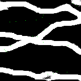
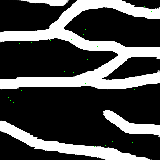
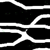
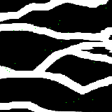
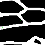
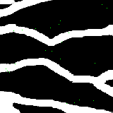
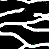
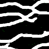
Finally, we evaluate our approach on the Subsurface dataset. We use the UNetResPAC architecture, since it performed the best on Texture data as exposed in Section 5.2. As previously, we simply set the regularization parameter at and, the network is trained for 40 epochs using the same experimental protocol. To evaluate the trade-off between the visual quality and the respect of the constraints, instead of FID we rather compute distances between visual Histograms of Oriented Gradients (see Section 4), extracted from real and generated samples. We also evaluate the visual quality of our approach with a distance between Local Binary Patterns. Indeed, Subsurface application lacks labelled data in order to learn a deep network classifier from which the FID score can be computed.
The obtained results are summarized in Tables 4 and 5. They are coherent with the previous experiments since the generated samples are diverse and have a low error regarding the constrained pixels. The conditioning have a limited impact on the visual quality of the generated samples and compares well to unconditional approaches [27]. Evaluation of the generated images using the domain-connectivity function highlights this fact on Figures 7 and 7 in the supplementary materials. Also examples of generated images by our approach pictured in Figure 9 (see appendix D) show that we preserve the visual quality and honor the constraints.
| Model | Best HOG | Best MSE | HOG at | MSE at | |
|---|---|---|---|---|---|
| best MSE | best HOG | ||||
| Subsurface | CGAN | 2.92e-4 | 0.2505 | 3.06e-4 | 1.1550 |
| Ours | 4.31e-4 | 0.0325 | 5.69e-4 | 0.2853 |
| Model | Best HOG | Best MSE | Best LBP | Best LBP | |
|---|---|---|---|---|---|
| (radius=1) | (radius=2) | ||||
| Subsurface | CGAN | 2.92e-4 | 0.2505 | 2.157 | 3.494 |
| Ours | 4.31e-4 | 0.0325 | 10.142 | 16.754 |
Conclusion
In this paper, we address the task of learning effective generative adversarial networks when only very few pixel values are known beforehand. To solve this pixel-wise conditioned GAN, we model the conditioning information under a probabilistic framework. This leads to the maximization of the likelihood of the constraints given a generated image. Under the assumption of a Gaussian distribution over the given pixels, we formulate an objective function composed of the conditional GAN loss function regularized by a -norm on pixel reconstruction errors. We describe the related optimization algorithm.
Empirical evidences illustrate that the proposed framework helps obtaining good image quality while best fulfilling the constraints compared to classical GAN approaches. We show that, if we include the PacGAN technique, this approach is compatible with fully-convolutional architectures and scales well to large images. We apply this approach to a common geological simulation task and show that it allows the generation of realistic samples which fulfill the prescribed constraints.
In future work, we plan to investigate other prior distributions for the given pixels as the Laplacian or -distribtutions. We are also interested in applying the developed approach to other applications or signals such as audio inpainting [40].
Acknowledgements
This research was supported by the CNRS PEPS I3A REGGAN project and the ANR-16-CE23-0006 grant Deep in France. We kindly thank the CRIANN for the provided high-computation facilities.
References
- [1] Ian Goodfellow, Jean Pouget-Abadie, Mehdi Mirza, Bing Xu, David Warde-Farley, Sherjil Ozair, Aaron Courville, and Yoshua Bengio. Generative adversarial nets. In Advances in neural information processing systems, pages 2672–2680, 2014.
- [2] Andrew Brock, Jeff Donahue, and Karen Simonyan. Large scale gan training for high fidelity natural image synthesis. arXiv preprint arXiv:1809.11096, 2018.
- [3] Mehdi Mirza and Simon Osindero. Conditional generative adversarial nets. arXiv preprint arXiv:1411.1784, 2014.
- [4] Phillip Isola, Jun-Yan Zhu, Tinghui Zhou, and Alexei A Efros. Image-to-image translation with conditional adversarial networks. In Proceedings of the IEEE conference on computer vision and pattern recognition, pages 1125–1134, 2017.
- [5] Ting-Chun Wang, Ming-Yu Liu, Jun-Yan Zhu, Andrew Tao, Jan Kautz, and Bryan Catanzaro. High-resolution image synthesis and semantic manipulation with conditional gans. In Proceedings of the IEEE conference on computer vision and pattern recognition, pages 8798–8807, 2018.
- [6] Deepak Pathak, Philipp Krahenbuhl, Jeff Donahue, Trevor Darrell, and Alexei A Efros. Context encoders: Feature learning by inpainting. In Proceedings of the IEEE conference on computer vision and pattern recognition, pages 2536–2544, 2016.
- [7] Ashish Bora, Eric Price, and Alexandros G Dimakis. Ambientgan: Generative models from lossy measurements. In International Conference on Learning Representations (ICLR), 2018.
- [8] Arthur Pajot, Emmanuel de Bezenac, and Patrick Gallinari. Unsupervised adversarial image reconstruction. In International Conference on Learning Representations, 2019.
- [9] Han Xiao, Kashif Rasul, and Roland Vollgraf. Fashion-mnist: a novel image dataset for benchmarking machine learning algorithms. arXiv preprint arXiv:1708.07747, 2017.
- [10] Alex Krizhevsky. Learning multiple layers of features from tiny images. In Technical report, University of Toronto, 2009.
- [11] Ziwei Liu, Ping Luo, Xiaogang Wang, and Xiaoou Tang. Deep learning face attributes in the wild. In Proceedings of International Conference on Computer Vision (ICCV), 2015.
- [12] Nikolay Jetchev, Urs Bergmann, and Roland Vollgraf. Texture synthesis with spatial generative adversarial networks. arXiv preprint arXiv:1611.08207, 2016.
- [13] Sebastien Strebelle. Conditional simulation of complex geological structures using multiple-point statistics. Mathematical Geology, 34(1):1–21, Jan 2002.
- [14] Eric Laloy, Romain Hérault, Diederik Jacques, and Niklas Linde. Training-image based geostatistical inversion using a spatial generative adversarial neural network. Water Resources Research, 54(1):381–406, 2018.
- [15] Dingdong Yang, Seunghoon Hong, Yunseok Jang, Tiangchen Zhao, and Honglak Lee. Diversity-sensitive conditional generative adversarial networks. In International Conference on Learning Representations, 2019.
- [16] Zinan Lin, Ashish Khetan, Giulia Fanti, and Sewoong Oh. Pacgan: The power of two samples in generative adversarial networks. In Advances in Neural Information Processing Systems, pages 1498–1507, 2018.
- [17] Raymond A Yeh, Chen Chen, Teck-Yian Lim, Alexander G Schwing, Mark Hasegawa-Johnson, and Minh N Do. Semantic image inpainting with deep generative models. In CVPR, volume 2, page 4, 2017.
- [18] Jiahui Yu, Zhe Lin, Jimei Yang, Xiaohui Shen, Xin Lu, and Thomas S Huang. Generative image inpainting with contextual attention. arXiv preprint arXiv:1801.07892, 2018.
- [19] Ugur Demir and Gozde Unal. Patch-based image inpainting with generative adversarial networks. arXiv preprint arXiv:1803.07422, 2018.
- [20] Yan Wu, Mihaela Rosca, and Timothy Lillicrap. Deep compressed sensing. In Proceedings of the 36th International Conference on Machine Learning, 2019.
- [21] Emmanuel J. Candes and Terrence Tao. Decoding by linear programming. IEEE Transactions on Information Theory, 51(12):4203–4215, Dec 2005.
- [22] Lawrence D Brown. Fundamentals of statistical exponential families: with applications in statistical decision theory. Ims, 1986.
- [23] Yann LeCun, Léon Bottou, Yoshua Bengio, and Patrick Haffner. Gradient-based learning applied to document recognition. Proceedings of the IEEE, 86(11):2278–2324, 1998.
- [24] Luca Oneto. Model Selection and Error Estimation in a Nutshell, pages 25–31. Springer International Publishing, Cham, 2020.
- [25] Alec Radford, Luke Metz, and Soumith Chintala. Unsupervised representation learning with deep convolutional generative adversarial networks. arXiv preprint arXiv:1511.06434, 2015.
- [26] Fisher Yu and Vladlen Koltun. Multi-scale context aggregation by dilated convolutions. arXiv preprint arXiv:1511.07122, 2015.
- [27] Cyprien Ruffino, Romain Hérault, Eric Laloy, and Gilles Gasso. Dilated spatial generative adversarial networks for ergodic image generation. In Conférence sur l’Apprentissage, 2018.
- [28] Jun-Yan Zhu, Taesung Park, Phillip Isola, and Alexei A Efros. Unpaired image-to-image translation using cycle-consistent adversarial networks. In Proceedings of the IEEE international conference on computer vision, pages 2223–2232, 2017.
- [29] Olaf Ronneberger, Philipp Fischer, and Thomas Brox. U-net: Convolutional networks for biomedical image segmentation. In International Conference on Medical image computing and computer-assisted intervention, pages 234–241. Springer, 2015.
- [30] Kaiming He, Xiangyu Zhang, Shaoqing Ren, and Jian Sun. Deep residual learning for image recognition. In Proceedings of the IEEE conference on computer vision and pattern recognition, pages 770–778, 2016.
- [31] Lucas Theis, Aäron van den Oord, and Matthias Bethge. A note on the evaluation of generative models. arXiv preprint arXiv:1511.01844, 2015.
- [32] Martin Heusel, Hubert Ramsauer, Thomas Unterthiner, Bernhard Nessler, and Sepp Hochreiter. Gans trained by a two time-scale update rule converge to a local nash equilibrium. In Advances in Neural Information Processing Systems, pages 6626–6637, 2017.
- [33] Tim Salimans, Ian Goodfellow, Wojciech Zaremba, Vicki Cheung, Alec Radford, and Xi Chen. Improved techniques for training gans. In Advances in Neural Information Processing Systems, pages 2234–2242, 2016.
- [34] Shane Barratt and Rishi Sharma. A note on the inception score. arXiv preprint arXiv:1801.01973, 2018.
- [35] Christian Szegedy, Vincent Vanhoucke, Sergey Ioffe, Jon Shlens, and Zbigniew Wojna. Rethinking the inception architecture for computer vision. In Proceedings of the IEEE conference on computer vision and pattern recognition, pages 2818–2826, 2016.
- [36] Mircea Cimpoi, Subhransu Maji, Iasonas Kokkinos, Sammy Mohamed, , and Andrea Vedaldi. Describing textures in the wild. In Proceedings of the IEEE Conf. on Computer Vision and Pattern Recognition (CVPR), 2014.
- [37] Navneet Dalal and Bill Triggs. Histograms of Oriented Gradients for Human Detection. In 2005 IEEE Computer Society Conference on Computer Vision and Pattern Recognition (CVPR’05), volume 1, pages 886–893. IEEE, 2005.
- [38] Matti Pietikäinen, Abdenour Hadid, Guoying Zhao, and Timo Ahonen. Computer Vision Using Local Binary Patterns, volume 40 of Computational Imaging and Vision. Springer London, London, 2011.
- [39] Laurent Lemmens, Bart Rogiers, Mieke De Craen, Eric Laloy, Diederik. Jacques, Marijeke Huysmans, and al. Effective structural descriptors for natural and engineered radioactive waste confinement barrier, 2017.
- [40] Andrés Marafioti, Nathanaël Perraudin, Nicki Holighaus, and Piotr Majdak. A context encoder for audio inpainting. arXiv preprint arXiv:1810.12138, 2018.
- [41] Sergey Ioffe and Christian Szegedy. Batch normalization: Accelerating deep network training by reducing internal covariate shift. arXiv preprint arXiv:1502.03167, 2015.
- [42] Dmitry Ulyanov, Andrea Vedaldi, and Victor Lempitsky. Instance normalization: The missing ingredient for fast stylization. arXiv preprint arXiv:1607.08022, 2016.
Appendix A Details of the datasets
| Dataset | Size (in pixels) | Training set | Validation set | Test set |
|---|---|---|---|---|
| FashionMNIST | 28x28 | 55,000 | 5,000 | 10,000 |
| Cifar-10 | 32x32 | 55,000 | 5,000 | 10,000 |
| CelebA | 128x128 | 80,000 | 5,000 | 15,000 |
| Texture | 160x160 | 20,000 | 2,000 | 4,000 |
| Subsurface | 160x160 | 20,000 | 2,000 | 4,000 |
Additional information:
-
•
For FashionMNIST and Cifar-10, we keep the original train/test split and then sample 5000 images from the training set that act as validation samples.
-
•
For the Texture dataset, we sample patches randomly from a 3840x2400 image of a brick wall.
Appendix B Detailed deep architectures
B.1 DCGAN for FashionMNIST
| Layer type | Units | Scaling | Activation | Output shape |
|---|---|---|---|---|
| Input z | - | - | - | 7x7 |
| Input y | - | - | - | 28x28 |
| Dense | 343 | - | ReLU | 7x7 |
| Conv2DTranspose | 128 3x3 | x2 | ReLU | 14x14 |
| Conv2DTranspose | 64 3x3 | x2 | ReLU | 28x28 |
| Conv2DTranspose | 1 3x3 | x1 | tanh | 28x28 |
| Input x | - | - | - | 28x28 |
| Input y | - | - | - | 28x28 |
| Conv2D | 64 3x3 | x1/2 | LeakyReLU | 14x14 |
| Conv2D | 128 3x3 | x1/2 | LeakyReLU | 7x7 |
| Conv2D | 1 3x3 | x1 | tanh | 28x28 |
| Dense | 1 | - | Sigmoid | 1 |
Additional information:
-
•
Batch normalization[41] is applied across all the layers
-
•
A Gaussian noise is applied to the input of the discriminator
B.2 UNet-Res for CIFAR10
| Layer type | Units | Scaling | Activation | Output shape |
|---|---|---|---|---|
| Input y | - | - | - | 32x32 |
| Conv2D* | 64 5x5 | x1 | ReLU | 32x32 |
| Conv2D* | 128 3x3 | x1/2 | ReLU | 16x16 |
| Conv2D* | 256 3x3 | x1/2 | ReLU | 8x8 |
| Input z | - | - | - | 8x8 |
| Dense | 256 | - | ReLU | 8x8 |
| Residual block | 3x256 3x3 | x1 | ReLU | 8x8 |
| Residual block | 3x256 3x3 | x1 | ReLU | 8x8 |
| Residual block | 3x256 3x3 | x1 | ReLU | 8x8 |
| Residual block | 3x256 3x3 | x1 | ReLU | 8x8 |
| Conv2DTranspose* | 256 3x3 | x2 | ReLU | 16x16 |
| Conv2DTranspose* | 128 3x3 | x2 | ReLU | 32x32 |
| Conv2DTranspose* | 64 3x3 | x1 | ReLU | 32x32 |
| Conv2D | 3 3x3 | x1 | tanh | 32x32 |
| Input x | - | - | - | 32x32 |
| Input y | - | - | - | 32x32 |
| Conv2D | 64 3x3 | x1/2 | LeakyReLU | 16x16 |
| Conv2D | 128 3x3 | x1/2 | LeakyReLU | 8x8 |
| Conv2D | 256 3x3 | x1/2 | LeakyReLU | 4x4 |
| Dense | 1 | - | Sigmoid | 1 |
Additional information:
-
•
Instance normalization[42] is applied across all the layers instead of Batch normalization. This is involved by the use of the PacGAN technique.
-
•
A Gaussian noise is applied to the input of the discriminator
-
•
The layers noted with an asterisk are linked with a skip-connection
B.3 UNet-Res for CelebA
| Layer type | Units | Scaling | Activation | Output shape |
|---|---|---|---|---|
| Input y | - | - | - | 128x128 |
| Conv2D | 64 5x5 | x1 | ReLU | 128x128 |
| Conv2D* | 128 3x3 | x1/2 | ReLU | 64x64 |
| Conv2D* | 256 3x3 | x1/2 | ReLU | 32x32 |
| Conv2D* | 512 3x3 | x1/2 | ReLU | 16x16 |
| Input z | - | - | - | 16x16 |
| Dense | 256 | - | ReLU | 16x16 |
| Residual block | 3x256 3x3 | x1 | ReLU | 16x16 |
| Residual block | 3x256 3x3 | x1 | ReLU | 16x16 |
| Residual block | 3x256 3x3 | x1 | ReLU | 16x16 |
| Residual block | 3x256 3x3 | x1 | ReLU | 16x16 |
| Residual block | 3x256 3x3 | x1 | ReLU | 16x16 |
| Residual block | 3x256 3x3 | x1 | ReLU | 16x16 |
| Conv2DTranspose* | 256 3x3 | x2 | ReLU | 32x32 |
| Conv2DTranspose* | 128 3x3 | x2 | ReLU | 64x64 |
| Conv2DTranspose* | 64 5x5 | x2 | ReLU | 128x128 |
| Conv2D | 3 3x3 | x1 | tanh | 128x128 |
| Input x | - | - | - | 128x128 |
| Input y | - | - | - | 128x128 |
| Conv2D | 64 3x3 | x1/2 | LeakyReLU | 64x64 |
| Conv2D | 128 3x3 | x1/2 | LeakyReLU | 32x32 |
| Conv2D | 256 3x3 | x1/2 | LeakyReLU | 16x16 |
| Conv2D | 512 3x3 | x1/2 | LeakyReLU | 32x32 |
| Dense | 1 | - | Sigmoid | 1 |
This network follows the same additional setup as described in Appendix (B.2).
B.4 Architectures for Texture
B.4.1 PatchGAN discriminator
| Layer type | Units | Scaling | Activation | Output shape |
|---|---|---|---|---|
| Input x | - | - | - | 160x160 |
| Input y | - | - | - | 160x160 |
| Conv2D | 64 3x3 | x1/2 | LeakyReLU | 80x80 |
| Conv2D | 128 3x3 | x1/2 | LeakyReLU | 40x40 |
| Conv2D | 256 3x3 | x1/2 | LeakyReLU | 20x20 |
| Conv2D | 512 3x3 | x1/2 | LeakyReLU | 10x10 |
B.4.2 UpDil Texture
| Layer type | Units | Scaling | Activation | Output shape |
|---|---|---|---|---|
| Input z | - | - | - | 20x20 |
| Conv2DTranspose | 256 3x3 | x2 | ReLU | 40x40 |
| Conv2DTranspose | 128 3x3 | x2 | ReLU | 80x80 |
| Conv2DTranspose | 64 3x3 | x2 | ReLU | 160x160 |
| Input y | - | - | - | 160x160 |
| Conv2D | 64 3x3 dil. 1 | x1 | ReLU | 160x160 |
| Conv2D | 128 3x3 dil. 2 | x1 | ReLU | 160x160 |
| Conv2D | 256 3x3 dil. 3 | x1 | ReLU | 160x160 |
| Conv2D | 512 3x3 dil. 4 | x1 | ReLU | 160x160 |
| Conv2D | 3 3x3 | x1 | tanh | 160x160 |
B.4.3 UpEncDec Texture
| Layer type | Units | Scaling | Activation | Output shape |
|---|---|---|---|---|
| Input z | - | - | - | 20x20 |
| Conv2DTranspose | 256 3x3 | x2 | ReLU | 40x40 |
| Conv2DTranspose | 128 3x3 | x2 | ReLU | 80x80 |
| Conv2DTranspose | 64 5x5 | x2 | ReLU | 160x160 |
| Input* y | - | - | - | 160x160 |
| Conv2D* | 64 3x3 | x1/2 | ReLU | 80x80 |
| Conv2D* | 128 3x3 | x1/2 | ReLU | 40x40 |
| Conv2D | 256 3x3 | x1/2 | ReLU | 20x20 |
| Conv2DTranspose* | 256 3x3 | x2 | ReLU | 40x40 |
| Conv2DTranspose* | 128 3x3 | x2 | ReLU | 80x80 |
| Conv2DTranspose* | 64 3x3 | x2 | ReLU | 160x160 |
| Conv2D | 3 3x3 | x1 | tanh | 160x160 |
B.4.4 UNet Texture
| Layer type | Units | Scaling | Activation | Output shape |
|---|---|---|---|---|
| Input y | - | - | - | 160x160 |
| Conv2D | 64 5x5 | x1 | ReLU | 160x160 |
| Conv2D* | 128 3x3 | x1/2 | ReLU | 80x80 |
| Conv2D* | 256 3x3 | x1/2 | ReLU | 40x40 |
| Conv2D* | 512 3x3 | x1/2 | ReLU | 20x20 |
| Input z | - | - | - | 20x20 |
| Conv2DTranspose* | 256 3x3 | x2 | ReLU | 40x40 |
| Conv2DTranspose* | 128 3x3 | x2 | ReLU | 80x80 |
| Conv2DTranspose* | 64 5x5 | x2 | ReLU | 160x160 |
| Conv2D | 3 3x3 | x1 | tanh | 160x160 |
B.4.5 Res Texture
| Layer type | Units | Scaling | Activation | Output shape |
|---|---|---|---|---|
| Input y | - | - | - | 160x160 |
| Conv2D | 64 5x5 | x1 | ReLU | 160x160 |
| Conv2D | 128 3x3 | x1/2 | ReLU | 80x80 |
| Conv2D | 256 3x3 | x1/2 | ReLU | 40x40 |
| Conv2D | 512 3x3 | x1/2 | ReLU | 20x20 |
| Input z | - | - | - | 20x20 |
| Residual block | 3x256 3x3 | x1 | ReLU | 20x20 |
| Residual block | 3x256 3x3 | x1 | ReLU | 20x20 |
| Residual block | 3x256 3x3 | x1 | ReLU | 20x20 |
| Residual block | 3x256 3x3 | x1 | ReLU | 20x20 |
| Residual block | 3x256 3x3 | x1 | ReLU | 20x20 |
| Residual block | 3x256 3x3 | x1 | ReLU | 20x20 |
| Conv2DTranspose | 256 3x3 | x2 | ReLU | 40x40 |
| Conv2DTranspose | 128 3x3 | x2 | ReLU | 80x80 |
| Conv2DTranspose | 64 5x5 | x2 | ReLU | 160x160 |
| Conv2D | 3 3x3 | x1 | tanh | 160x160 |
B.4.6 UNet-Res Texture
| Layer type | Units | Scaling | Activation | Output shape |
|---|---|---|---|---|
| Input y | - | - | - | 160x160 |
| Conv2D | 64 5x5 | x1 | ReLU | 160x160 |
| Conv2D* | 128 3x3 | x1/2 | ReLU | 80x80 |
| Conv2D* | 256 3x3 | x1/2 | ReLU | 40x40 |
| Conv2D* | 512 3x3 | x1/2 | ReLU | 20x20 |
| Input z | - | - | - | 20x20 |
| Residual block | 3x256 3x3 | x1 | ReLU | 20x20 |
| Residual block | 3x256 3x3 | x1 | ReLU | 20x20 |
| Residual block | 3x256 3x3 | x1 | ReLU | 20x20 |
| Residual block | 3x256 3x3 | x1 | ReLU | 20x20 |
| Residual block | 3x256 3x3 | x1 | ReLU | 20x20 |
| Residual block | 3x256 3x3 | x1 | ReLU | 20x20 |
| Conv2DTranspose* | 256 3x3 | x2 | ReLU | 40x40 |
| Conv2DTranspose* | 128 3x3 | x2 | ReLU | 80x80 |
| Conv2DTranspose* | 64 5x5 | x2 | ReLU | 160x160 |
| Conv2D | 3 3x3 | x1 | tanh | 160x160 |
As for Cifar10, this network follows the same additional setup described in Appendix (B.2).
Appendix C Domain-specific metrics for underground soil generation
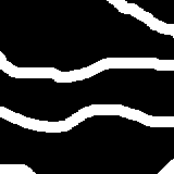
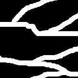
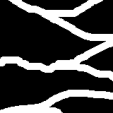
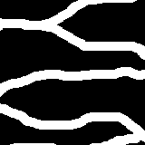
In this section, we compute the connectivity function [39] of generated soil image, a domain-specific metric, which is the probability that a continuous pixel path exists between two pixels of the same value (called Facies) in a given direction and a given distance (called Lag). This connectivity function should be similar to the one obtained on real-world samples. In this application, the connectivity function models the probability that two given pixels are from the same sand brick or clay matrix zone.


We sampled 100 real and 100 generated images using the UNetResPAC architecture (see Section 4.2) on which the connectivity function was evaluated for both the CGAN and our approach. The obtained graphs are shown respectively in Figures 6 and 7.
The blue curves are the mean value for the real samples, and the blue dashed curves are the minimum and maximum values on these samples. The green curves are the connectivity functions for each of the 100 synthetic samples and the red curves are their mean connectivity functions. From these curves we observe that that our approach has similar connectivity functions as the CGAN approach while being significantly better at respecting the given constraints (see Section Table 4).
Appendix D Additional samples from the Texture and Subsurface datasets
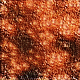
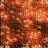
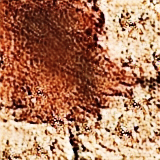
In this section, we show some samples generated with the UNetResPAC architecture, which performs the best in our experiments (see Section 5) compared to real images sampled from the Texture (Figure 8) and Subsurface (Figure 9) datasets. For the generated samples, the enforced pixel constraints are colored in the images, green corresponding to a squared error less than and red otherwise.
Texture: Real samples
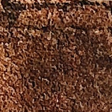
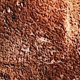
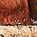
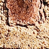
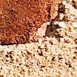
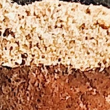

Texture: Generated samples
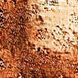
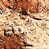
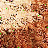
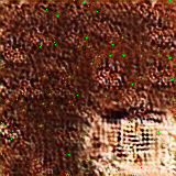


Subsurface: Real samples

Subsurface: Generated samples