Spontaneous emission and energy shifts of a Rydberg rubidium atom close to an optical nanofiber

Abstract

In this paper, we report on numerical calculations of the spontaneous emission rates and Lamb shifts of a ${}^{87}\text{Rb}$ atom in a Rydberg-excited state $\left(n\leq 30\right)$ located close to a silica optical nanofiber. We investigate how these quantities depend on the fiber’s radius, the distance of the atom to the fiber, the direction of the atomic angular momentum polarization as well as the different atomic quantum numbers. We also study the contribution of quadrupolar transitions, which may be substantial for highly polarizable Rydberg states. Our calculations are performed in the macroscopic quantum electrodynamics formalism, based on the dyadic Green’s function method. This allows us to take dispersive and absorptive characteristics of silica into account; this is of major importance since Rydberg atoms emit along many different transitions whose frequencies cover a wide range of the electromagnetic spectrum. Our work is an important initial step towards building a Rydberg atom-nanofiber interface for quantum optics and quantum information purposes.

I Introduction

Within the last two decades, the strong dipole-dipole interaction experienced by two neighbouring Rydberg-excited atoms (GA94, ) has become the main ingredient for many atom-based quantum information protocol proposals (SWM10, ). This interaction can be so large as to forbid the simultaneous resonant excitation of two atoms if their separation is less than a specific distance, called the blockade radius (TFS04, ), which typically depends on the intensity of the laser excitation and the interaction between the Rydberg atoms (LWR09, ). The discovery of this “Rydberg blockade” phenomenon (LFC01, ; TFS04, ; SRA04, ; CRB05, ; AVG98, ; VVZ06, ) paved the way for a new encoding scheme using atomic ensembles as collective quantum registers (LFC01, ; BMS07, ; BMM07, ; BPS08, ) and repeaters (BCA12, ; ZMH10, ; HHH10, ).

Scalability is one of the crucial requirements for quantum devices (DiV00, ) and interfacing atomic ensembles into a quantum network is a possible way to reach this goal. Photons naturally appear as ideal information carriers and the photon-based protocols considered so far include free-space (PM09, ), or guided propagation through optical fibers (BCA12, ). The former has the advantage of being relatively easy to implement, but presents the drawback of strong losses. The latter requires a cavity quantum electrodynamics setup, which is experimentally more involved. An alternative option would be to use optical nanofibers. Such fibers have recently received much attention (SGH17, ; NGN16, ) because the coupling to the evanescent guided modes of a nanofiber allows for easy-to-implement atom trapping (BHK04, ; KBH04, ; VRS10, ) and detection (NMM07, ; DWM09, ; KSB17, ). This coupling increases in strength as the fiber diameter reduces and the atoms approach the fiber surface. It has also been shown that energy could be exchanged between two distant atoms via the guided modes of the fiber (KDN05, ). This suggests that optical nanofibers could play the role of a communication channel between the nodes of an atomic quantum network consisting of Rydberg-excited atomic ensembles.

In the perspective of building a quantum network based on Rydberg-blockaded atomic ensembles linked via an optical nanofiber, we recently studied the spontaneous emission of a highly-excited (Rydberg) sodium atom in the neighbourhood of an optical nanofiber made of silica (SZL19, ). To be more specific, we investigated how the atomic emission rates into the guided and radiative fiber modes are influenced by the radius of the fiber, the distance of the atom to the fiber and the symmetry of the Rydberg state. In the spirit of Ref. (KDB05, ), we used the so-called mode function description of the nanofiber which does not allow one to take absorption and dispersion of the fiber into account. This point is critical with highly excited atoms since they can de-excite along many transitions of different frequencies for which the fiber index is different and potentially complex. This forced us, in Ref. (SZL19, ), to restrict ourselves to Rydberg levels of moderate principal numbers so that the frequencies of the transitions involved remain in a nondispersive and nonabsorptive window of the silica spectrum. By contrast, here, we resort to the framework of macroscopic quantum electrodynamics based on the dyadic Green’s function (NH12, ; Buh12, ). This formalism enables us to take the exact refractive index of silica into account and relaxes all constraints on the transitions we can address. This framework also offers a natural way to compute not only spontaneous emission rates, but also Lamb shifts and (resonant and nonresonant) electromagnetic forces the atom is subject to.

In this article, we present the numerical results we obtained with this approach for a rubidium atom prepared in a Rydberg-excited state $\left|n\leq 30;L=S,P,D;JFM_{F}\right\rangle$ in the vicinity of a multimode silica optical nanofiber. We chose ${}^{87}\text{Rb}$ as it is commonly used in Rydberg atom experiments, like in the recent experimental work on Rydberg generation next to a nanofiber (RRK19, ). In particular, we show that a non-negligible fraction of spontaneously emitted light is guided along the fiber and study how it depends on principal quantum number, $n$, the radius of the nanofiber, $a$, the distance of the atom to the nanofiber axis, $R$, and the direction of angular momentum polarization. Interestingly, when the quantum and fiber axes do not coincide, spontaneous emission becomes directional, as already noticed for low-excited atoms (KR14, ; SBC15, ) due to the peculiar polarization structure of the field in the neighbourhood of the fiber. As shown by our calculations, this effect is particularly strong for photons emitted into the fiber-guided modes and persists even for high principal quantum numbers, $n$. This is promising in view of potential applications in chiral quantum information protocols (LMS17, ) based on a Rydberg-atom-nanofiber interface. We also address Lamb shifts and associated dispersion forces that arise. In particular, we show that, as $n$ increases, the contribution of quadrupolar transitions becomes more and more important. This contrasts with spontaneous emission rates for which quadrupolar transitions have negligible influence.

The article is organized as follows. In Sec. II we present the system and introduce the important formulae used in our calculations. In Sec. III we present and interpret our numerical results for spontaneous emission rates, Lamb shifts and forces. We conclude in Sec. IV and give perspectives of our work. More technical details of our work can be found in Appendices.

II System and methods

In this article, we consider a rubidium atom, ${}^{87}\text{Rb}$, initially prepared in a highly-excited (Rydberg) level $n\leq 30$, located at a distance $R$ from the axis of a silica nanofiber of radius $a$. Our goal is to investigate how the fiber modifies the atomic spontaneous emission rates, the Lamb shifts, and the forces on the atom. To be more specific, we want to study the influence of: i) the radius of the fiber, ii) the distance of the atom to the fiber, iii) the different quantum numbers of the Rydberg state $\left|nLJFM_{F}\right\rangle$, in particular the principal quantum number $n$, and iv) the direction of angular momentum polarization on these properties. On Fig. 1, we define the reference frame $\left(Oxyz\right)$ and the associated unitary basis $\left(\vec{e}_{x},\vec{e}_{y},\vec{e}_{z}\right)$. The origin $O$ is chosen as the projection of the atomic center of mass onto the fiber axis, the $z$-axis coincides with the fiber axis, and the $x$-axis joins the origin $O$ and the center of mass of the atom. In this basis, the position vector of the atom is $\vec{R}=R\vec{e}_{x}$. For future reference we also introduce the cylindrical basis $\left(\vec{e}_{\rho},\vec{e}_{\phi},\vec{e}_{z}\right)$ on Fig. 1, defined by $\vec{e}_{\rho}=\cos\phi\vec{e}_{x}+\sin\phi\vec{e}_{y}$, $\vec{e}_{\phi}=-\sin\phi\vec{e}_{x}+\cos\phi\vec{e}_{y}$.

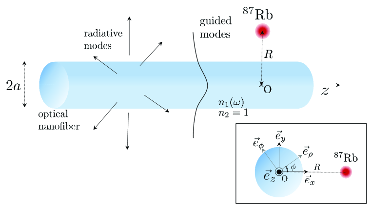
Figure 1: A ${}^{87}\text{Rb}$ atom located at a distance, $R$, from the axis of an optical nanofiber of radius, $a$. The refractive index $n_{1}\left(\omega\right)$ for silica is obtained by a numerical fit of the experimental data taken from (Pal98, ). Outside the fiber, the refractive index is $n_{2}=1$. The axis of the nanofiber is arbitrarily chosen as the $z$-axis. The cylindrical coordinates $\left(\rho,\phi,z\right)$ and frame $\left(\vec{e}_{\rho},\vec{e}_{\phi},\vec{e}_{z}\right)$ are introduced in the inset.

We shall resort to the theoretical framework of macroscopic quantum electrodynamics (NH12, ; Buh12, ), which allows one to consider the exact frequency-dependent form of the electric susceptibility of silica, obtained through a fit of experimental data given in (Pal98, ). This formalism is based on the dyadic Green’s function $\overline{\overline{G}}\left(\vec{r},\vec{r}^{\prime},\omega\right)$, which is the solution to the Helmholtz equation

$$\left[\vec{\nabla}\times\vec{\nabla}\times-\varepsilon\left(\vec{r},\omega\right)\frac{\omega^{2}}{c^{2}}\right]\overline{\overline{G}}\left(\vec{r},\vec{r}^{\prime},\omega\right)=\delta\left(\vec{r}-\vec{r}^{\prime}\right)\overline{\overline{I}},$$ (1)

where $\varepsilon\left(\vec{r},\omega\right)$ is the relative electric permittivity of the medium at the position $\vec{r}$ and frequency $\omega$ while $\overline{\overline{I}}$ is the unit dyadic (Tai94, ). The solution of Eq. (1) in the case of a cylindrical nanofiber is given in Appendix A. There exist two useful decompositions of $\overline{\overline{G}}$ : i) $\overline{\overline{G}}=\overline{\overline{G}}_{0}+\overline{\overline{G}}_{\text{sc}}$ where $\overline{\overline{G}}_{0}$ is the vacuum component, and $\overline{\overline{G}}_{\text{sc}}$ the scattering contribution due to the presence of the nanofiber and ii) $\overline{\overline{G}}=\overline{\overline{G}}_{\text{g}}+\overline{\overline{G}}_{\text{r}}$ where $\overline{\overline{G}}_{\text{g,r}}$ are the respective contributions of the guided and radiative modes.

We summarize below the main formulae we used to obtain the results presented in the next section, the derivation of which can be found in (Buh12, ; BKW04, ). The spontaneous emission rate, $\Gamma_{n}$, from an excited state, $\left|n\right\rangle$, is given by the sum, $\Gamma_{n}=\sum_{k<n}\Gamma_{nk}$, of rates

$$\Gamma_{nk} = \frac{2\mu_{0}}{\hbar}\omega_{nk}^{2}\vec{d}_{nk}\cdot\mathrm{Im}\left[\overline{\overline{G}}\left(\vec{R},\vec{R},\omega_{nk}\right)\right]\cdot\vec{d}_{kn}$$ (2)

relative to the different transitions $\left|n\right\rangle\rightarrow\left|k\right\rangle$ for $k<n$, where $\omega_{nk}$ and $\vec{d}_{nk}\equiv\left\langle n\left|\hat{\vec{d}}\right|k\right\rangle$ denote the bare frequency and the dipole matrix element of the transition $\left|k\right\rangle\rightarrow\left|n\right\rangle$, respectively.

In the same way, the Lamb shift, $\delta\omega_{n}$, of an excited state, $\left|n\right\rangle$, is given by the sum, $\delta\omega_{n}=\sum_{k}\delta\omega_{nk}$, of all energy shifts induced by the different transitions $\left|n\right\rangle\rightarrow\left|k\right\rangle$, for arbitrary $k\neq n$, with

$$\delta\omega_{nk} = -\frac{\mu_{0}}{\hbar\pi}\mathcal{P}\left(\intop_{0}^{+\infty}\mathrm{d}\omega\leavevmode\nobreak\ \frac{\omega^{2}}{\omega-\omega_{nk}}\vec{d}_{nk}\cdot\mathrm{Im}\left[\overline{\overline{G}}\left(\vec{R},\vec{R},\omega\right)\right]\cdot\vec{d}_{kn}\right)$$ (3)

where $\mathcal{P}$ denotes the Cauchy principal value. Here, we shall use the non-retarded approximation (EBS11, )

$$\delta\omega_{nk} \approx -\frac{1}{2\hbar\epsilon_{0}}\vec{d}_{nk}\cdot\overline{\overline{\Gamma}}_{0}\left(\vec{R}\right)\cdot\vec{d}_{kn}$$ (4)

where $\overline{\overline{\Gamma}}_{0}\left(\vec{R}\right)=\lim_{\omega\rightarrow 0}\frac{\omega^{2}}{c^{2}}\overline{\overline{G}}\left(\vec{R},\vec{R},\omega\right)$. This approximation is particularly suited for Rydberg atoms, since the main contributions to the Lamb shift are due to transitions to neighbouring states, therefore of long wavelengths.

Finally, the average resonant and nonresonant forces on an atom initially in the state $\left|n\right\rangle$, evaluated at $t=0$, are given by (see Appendix B)

$$\vec{F}^{\text{res}}\left(t=0\right) = \sum_{k}\left[\mu_{0}\omega_{nk}^{2}\vec{\nabla}_{\vec{r}}\left.\left[\vec{d}_{nk}\cdot\overline{\overline{G}}_{\text{sc}}\left(\vec{r},\vec{R},\omega_{nk}\right)\cdot\vec{d}_{kn}\right]\right|_{\vec{r}=\vec{R}}+\text{c.c.}\right]$$ (5)

$$\vec{F}^{\text{nonres}}\left(t=0\right) = -\frac{\mu_{0}}{\pi}\intop_{0}^{+\infty}\mathrm{d}\xi\leavevmode\nobreak\ \xi^{2}\frac{\omega_{kn}}{\omega_{kn}^{2}+\xi^{2}}\nabla_{\vec{r}}\left[\vec{d}_{nk}\cdot\overline{\overline{G}}_{\text{sc}}\left(\vec{r},\vec{R},\mathrm{i}\xi\right)|_{\vec{r}=\vec{R}}\cdot\vec{d}_{kn}\right].$$ (6)

where $\vec{\nabla}_{\vec{r}}$ acts on the spatial variable, $\vec{r}$.

III Numerical results and discussion

In this section we present and interpret the numerical results we obtained for spontaneous emission rates and Lamb shifts of a ${}^{87}\text{Rb}$ atom in the vicinity of a silica optical nanofiber. In particular, we investigate the effect of the distance, $R$, from the atom to the fiber axis, the fiber radius, $a$, and the atomic quantum numbers. We also study the influence of the direction of angular momentum polarization on the strength and directionality of spontaneous emission from a Rydberg level, specifically towards the guided modes. Finally, we address quadrupolar transitions, which, a priori, may have a substantial influence on Rydberg atom emission properties in view of their high polarizability.

III.1 Spontaneous emission rates

We start the discussion with the results we obtained for spontaneous emission rates. In Secs. III.1.1-III.1.3, the quantization axis is implicitly chosen along the fiber axis $\left(Oz\right)$. In contrast, in Secs. III.1.4-III.1.5, we investigate the changes induced by other quantization axis choices. In some places, for pedagogical reasons, we shall resort to the so-called mode function approach (widely used in the works by F. Le Kien, see, e.g. (KBH04, )) as it offers a simple and illustrative way to physically interpret our results. However, we wish to emphasise that our calculations were performed using the (more general) Green’s function formalism, which allows one to account for dispersive and absorptive characteristics of the fiber.

III.1.1 Dependence on the distance, $R$, from the atom to the fiber axis

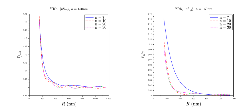
Figure 2: Spontaneous emission rates of an ${}^{87}\text{Rb}$ atom in the state $\left|nS_{\nicefrac{{1}}{{2}}}\right\rangle$ (with $n=7,10,20,30$) – dependence on the distance, $R$, from the atom to the nanofiber. We represent the ratios $\nicefrac{{\Gamma}}{{\Gamma_{0}}}$ (left), $\nicefrac{{\Gamma_{g}}}{{\Gamma}}$ (right) as functions of $R$. $\Gamma_{g}$ and $\Gamma_{r}$ denote the spontaneous emission rates towards the guided and radiative modes, respectively, $\Gamma\equiv\Gamma_{g}+\Gamma_{r}$ is the total spontaneous emission rate and $\Gamma_{0}$ the spontaneous emission rate in vacuum. The radius of the nanofiber is fixed at $a=150$ nm.

Figure 3: Spontaneous emission rates of an ${}^{87}\text{Rb}$ atom in the state $\left|nP_{\nicefrac{{3}}{{2}}},F=3,M_{F}=3\right\rangle$ (with $n=7,10,20,30$) – dependence on the distance, $R$, from the atom to the nanofiber. We represent the ratios $\nicefrac{{\Gamma}}{{\Gamma_{0}}}$ (left), $\nicefrac{{\Gamma_{g}}}{{\Gamma}}$ (right) as functions of $R$. $\Gamma_{g}$, $\Gamma_{r}$ denote the spontaneous emission rates into the guided and radiative modes, respectively, $\Gamma\equiv\Gamma_{g}+\Gamma_{r}$ is the total spontaneous emission rate and $\Gamma_{0}$ the spontaneous emission rate in vacuum. The radius of the nanofiber is fixed at $a=150$ nm.

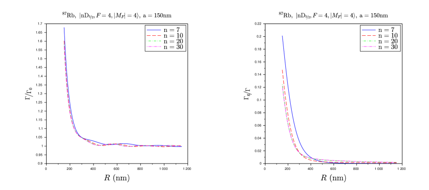
Figure 4: Spontaneous emission rates of an ${}^{87}\text{Rb}$ atom in the state $\left|nD_{\nicefrac{{5}}{{2}}},F=4,M_{F}=4\right\rangle$ (with $n=7,10,20,30$) – dependence on the distance, $R$, from the atom to the nanofiber. We represent the ratios $\nicefrac{{\Gamma}}{{\Gamma_{0}}}$ (left), $\nicefrac{{\Gamma_{g}}}{{\Gamma}}$ (right) as functions of $R$. $\Gamma_{g}$, $\Gamma_{r}$ denote the spontaneous emission rates into the guided and radiative modes, respectively, $\Gamma\equiv\Gamma_{g}+\Gamma_{r}$ is the total spontaneous emission rate and $\Gamma_{0}$ is the spontaneous emission rate in vacuum. The radius of the nanofiber is fixed at $a=150$ nm.

Figures 2, 3 and 4 show the variations with the distance, $R$, from the atom to the nanofiber axis of: i) the ratio $\nicefrac{{\Gamma}}{{\Gamma_{0}}}$ of the total spontaneous emission rate of the atom to the spontaneous emission rate in vacuum, ii) the ratio $\nicefrac{{\Gamma_{g}}}{{\Gamma}}$ of the spontaneous emission rate of the atom only into the guided modes to the total spontaneous emission rate for the states $\left|nS_{\nicefrac{{1}}{{2}}}\right\rangle$, $\left|nP_{\nicefrac{{3}}{{2}}},F=3,M_{F}=3\right\rangle$,

$\left|nD_{\nicefrac{{5}}{{2}}},F^{\prime}=4,M_{F^{\prime}}=4\right\rangle$, respectively, with $n=7,10,20,30$, and for a nanofiber radius $a=150\text{ nm}$.

$n$	7	10	20	30
$\left|nS_{\nicefrac{{1}}{{2}}}\right\rangle$	$1.132\times\mathrm{10}^{7}$	$2.375\times\mathrm{10}^{6}$	$1.662\times\mathrm{10}^{5}$	$4.120\times\mathrm{10}^{4}$
$\left|nP_{\nicefrac{{1}}{{2}}}\right\rangle$	$1.624\times\mathrm{10}^{6}$	$7.424\times\mathrm{10}^{5}$	$6.252\times\mathrm{10}^{4}$	$1.624\times\mathrm{10}^{4}$
$\left|nD_{\nicefrac{{5}}{{2}}},F=4,M_{F}=4\right\rangle$	$2.642\times\mathrm{10}^{6}$	$1.092\times\mathrm{10}^{6}$	$1.328\times\mathrm{10}^{5}$	$3.780\times\mathrm{10}^{4}$

Table 1: Theoretical values of the spontaneous emission rate, $\Gamma_{0}$, in vacuum of an ${}^{87}\text{Rb}$ atom in the states $|\mathrm{nS}_{1/2}\rangle$, $|\mathrm{nP}_{1/2}\rangle$ and $|\mathrm{nD}_{5/2},F=4,M_{F}=4\rangle$ for $n=7,10,20,30$ (in $\text{s}^{-1}$).

In all cases, close to the nanofiber, the total spontaneous emission is amplified when compared with its value in vacuum. This amplification vanishes as $R$ increases. The small Drexhage-like oscillations observed (D70, ) are due to the oscillatory behavior of the radiative modes themselves.

Close to the fiber, a non-negligible fraction of the spontaneous emission is captured by the guided modes. The strongest effect is obtained for $S$ and $D$ states, as already noted and interpreted in (SZL19, ). As $R$ increases, the guided modes are (quasi-)exponentially damped, hence the damping of $\Gamma_{g}$ itself.

The dependence with $n$ is less easy to interpret. Let us first note that $\Gamma$, $\Gamma_{g}$ and $\Gamma_{0}$ substantially decrease when the principal quantum number increases (see Table 1 for theoretical values of $\Gamma_{0}$). The ratios $\nicefrac{{\Gamma}}{{\Gamma_{0}}}$ and $\nicefrac{{\Gamma_{g}}}{{\Gamma}}$, however, keep the same order of magnitude and, therefore, the plots in Figs. 2, 3 and 4 for $n=7,10,20,30$ remain close to each other. In particular, for high values of $n$, the plots seem to tend to an asymptotic curve. This observation can be qualitatively understood as follows. We first note that, for high $n$, only a few transitions substantially contribute to the spontaneous emission rate. In the crude but practical two-level approximation, we assume the spontaneous emission rate is dominated by one transition $\left|n\right\rangle\rightarrow\left|k\right\rangle$ whose total spontaneous emission rate, spontaneous emission rate towards guided modes and spontaneous emission rate in vacuum are, respectively, given by

$$\Gamma_{nk} = \frac{2\mu_{0}}{\hbar}\omega_{nk}^{2}\vec{d}_{nk}\cdot\mathrm{Im}\left[\overline{\overline{G}}\left(\vec{R},\vec{R},\omega_{nk}\right)\right]\cdot\vec{d}_{kn}$$

$$\Gamma_{\text{g},nk} = \frac{2\mu_{0}}{\hbar}\omega_{nk}^{2}\vec{d}_{nk}\cdot\mathrm{Im}\left[\overline{\overline{G}}_{\text{g}}\left(\vec{R},\vec{R},\omega_{nk}\right)\right]\cdot\vec{d}_{kn}$$

$$\Gamma_{0,nk} = \frac{\omega_{nk}^{3}\vec{d}_{nk}^{2}}{3\pi\hbar\varepsilon_{0}c^{3}}.$$

For increasing $n$, $\omega_{nk}$ saturates, i.e., Rydberg levels are closer and closer in energy as the principal quantum number grows, and the terms $\omega_{nk}^{2}\mathrm{Im}\left[\overline{\overline{G}}\left(\vec{R},\vec{R},\omega_{nk}\right)\right]$ and $\omega_{nk}^{2}\mathrm{Im}\left[\overline{\overline{G}}_{g}\left(\vec{R},\vec{R},\omega_{nk}\right)\right]$, therefore, also saturate. Finally, since $\Gamma,\Gamma_{\text{g}},\Gamma_{0}\propto\left|\vec{d}_{nk}\right|^{2}$, the ratios $\nicefrac{{\Gamma}}{{\Gamma_{0}}}$ and $\nicefrac{{\Gamma_{g}}}{{\Gamma}}$ do not (substantially) depend on the dipole and saturate as $n$ increases.

III.1.2 Dependence on the fiber radius, $a$

Figure 5 shows the dependence on the fiber radius, $a$, of the ratio $\nicefrac{{\Gamma_{g}}}{{\Gamma}}$ for an ${}^{87}\text{Rb}$ atom in the states $\left|nS_{\nicefrac{{1}}{{2}}}\right\rangle$ (left), $\left|nP_{\nicefrac{{1}}{{2}}}\right\rangle$ (middle) and $\left|nD_{\nicefrac{{5}}{{2}}},F=4,\left|M_{F}\right|=4\right\rangle$ (right), with $n=\left(7,10,20,30\right)$. The atom is located at a distance $d=50\text{ nm}$ from the fiber surface, i.e., $R=a+50$ nm from the fiber axis. Note that the contributions of all guided modes are summed.

The ratio $\nicefrac{{\Gamma_{g}}}{{\Gamma}}$ exhibits the same qualitative behavior with respect to $a$ for $S$ and $D$ states, and $\left(\nicefrac{{\Gamma_{g}}}{{\Gamma}}\right)_{S,D}\approx 10\left(\nicefrac{{\Gamma_{g}}}{{\Gamma}}\right)_{P}$. Note that, for the states $\left|nS_{\nicefrac{{1}}{{2}}}\right\rangle$ and $\left|nP_{\nicefrac{{1}}{{2}}}\right\rangle$, the hyperfine states (recall $I=\frac{3}{2}$ for ${}^{87}\text{Rb}$) have the same $\Gamma_{g}$. This is not the case for $\left|nD_{\nicefrac{{5}}{{2}}}\right\rangle$ and in Fig. 5, we chose to represent the specific “edge” hyperfine state $\left|nD_{\nicefrac{{5}}{{2}}},F=4,M_{F}=4\right\rangle$.

The abrupt slope changes observed in all plots originate from the appearance of additional guided modes as $a$ increases. To be more explicit, the successive maxima of $\nicefrac{{\Gamma_{g}}}{{\Gamma}}$ can be interpreted as follows: i) As a function of the fiber radius, the amplitude of a specific guided mode at the location of the atom, i.e. at a distance $d$ from the fiber surface, exhibits a maximum for a specific value, denoted by $a_{max}\left(\omega,d\right)$, which depends both on the frequency of the mode and the distance, $d$. (Note that $a_{max}$ actually also depends on other characteristics of the mode such as polarization, and wavevector). ii) For a given atomic transition, of frequency, $\omega_{0}$, the coupling to a given mode reaches its maximum when $a=a_{max}\left(\omega_{0},d\right)$, hence a peak in $\nicefrac{{\Gamma_{g}}}{{\Gamma}}$.

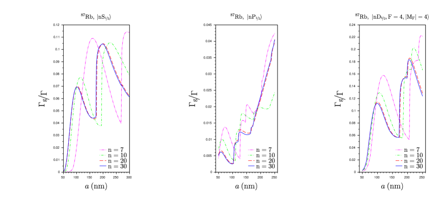
Figure 5: Spontaneous emission of an ${}^{87}\text{Rb}$ atom near an optical nanofiber – dependence on the fiber radius, $a$. We represent the ratio $\nicefrac{{\Gamma_{g}}}{{\Gamma}}$, for an ${}^{87}\text{Rb}$ atom in the states $\left|nS_{\nicefrac{{1}}{{2}}}\right\rangle$ (left), $\left|nP_{\nicefrac{{1}}{{2}}}\right\rangle$ (middle) and $\left|nD_{\nicefrac{{5}}{{2}}},F=4,\left|M_{F}\right|=4\right\rangle$ (right), with $n=\left(7,10,20,30\right)$, as a function of $a$. The atom is located 50 nm from the fiber (i.e., $R=a+$50 nm).

Figure 6 shows the dependence on the fiber radius, $a$, of the ratio $\nicefrac{{\Gamma_{g}}}{{\Gamma}}$ for an ${}^{87}\text{Rb}$ atom in the states $\left|30P_{\nicefrac{{3}}{{2}}},F=0\cdots 3,\left|M_{F}\right|=0\cdots F\right\rangle$ located at a distance $d=50$ nm from the fiber surface, i.e., $R=a+50$ nm from the fiber axis. As can be observed in the figure, though the different hyperfine magnetic sublevels for a given $F$ show the same qualitative behavior, the spontaneous emission towards the guided modes is stronger for states of higher $\left|M_{F}\right|$. This can be qualitatively understood as follows: i) Guided modes have a large (though not exclusive) transverse component, i.e., orthogonal to the fiber axis $\left(Oz\right)$ (see Fig. 1); ii) High coupling to the guided modes is, therefore, obtained for transitions corresponding to dipoles in the transverse plane $\left(Oxy\right)$; iii) The quantization axis being along the fiber axis, dipoles in the plane $\left(Oxy\right)$ correspond to $\sigma$-transitions: therefore, the stronger the weight of $\sigma$-transitions in the de-excitation of an excited state, the higher the spontaneous emission rate towards guided modes; iv) The higher the value of $\left|M_{F}\right|$, the stronger the weight of $\sigma$-transitions in the de-excitation of the state (this can be directly checked on $3j$-coefficients), therefore, the higher $\left|M_{F}\right|$, the higher the spontaneous emission rate towards guided modes.

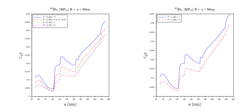
Figure 6: Spontaneous emission of an ${}^{87}\text{Rb}$ atom near an optical nanofiber – dependence on the fiber radius, $a$. We represent the ratio $\nicefrac{{\Gamma_{g}}}{{\Gamma}}$ for an ${}^{87}\text{Rb}$ atom in the states $\left|30P_{\nicefrac{{3}}{{2}}},F=0,2,3,\left|M_{F}\right|=0\cdots F\right\rangle$ (left) and $\left|30P_{\nicefrac{{3}}{{2}}},F=1,\left|M_{F}\right|=0\cdots F\right\rangle$ (right) as a function of $a$. The atom is located $50$ nm from the fiber (i.e., $R=a+50$ nm).

The same behavior can be observed and interpreted in Fig. 7 for the states

$\left|30D_{\nicefrac{{5}}{{2}}},F=1\cdots 4,\left|M_{F}\right|=0\cdots F\right\rangle$.

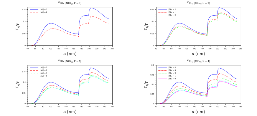
Figure 7: Spontaneous emission of an ${}^{87}\text{Rb}$ atom near an optical nanofiber – dependence on the fiber radius, $a$. We represent the ratio $\nicefrac{{\Gamma_{g}}}{{\Gamma}}$ for an ${}^{87}\text{Rb}$ atom in the states $\left|30D_{\nicefrac{{5}}{{2}}};F=1,\cdots,4;\left|M_{F}\right|=0\cdots F\right\rangle$ as a function of $a$. The atom is located at $50$ nm from the fiber (i.e., $R=a+50$ nm).

III.1.3 Role of quadrupolar transitions

Because of their polarizability, Rydberg atoms are very sensitive to electric fields and electric field inhomogeneities. It is, therefore, reasonable to expect quadrupolar transitions to play a role in the de-excitation of a Rydberg atom in the vicinity of an optical nanofiber where spatial variations of the field are very rapid. Following (KRN18, ; KD05, ; CS19, ), we calculate the correction due to electric quadrupolar transitions on the spontaneous emission rates of an ${}^{87}\text{Rb}$ atom in the state $\left|nS_{\nicefrac{{1}}{{2}}}\right\rangle$ located close to a silica optical nanofiber (see Appendix C for more details).

Figure 8 (left) shows the dependence on $n$ of the electric quadrupolar transition correction, $\Gamma_{r}^{Q}$, to the spontaneous emission rate into the radiative modes, for two values of the nanofiber radius, $a=100$ and 200 nm. To obtain the strongest effect, we fixed $R=a$, corresponding to the unrealistic situation in which the atom is located at the fiber surface. As expected, for smaller values of $a$, the field inhomogeneities are more pronounced and the effect of electric quadrupolar transitions is higher. Moreover, the contribution $\Gamma_{r}^{Q}$ decreases with increasing $n$, in the same way as the coupling to ground states that is responsible for the spontaneous emission.

The same observations can be made from Fig. 8 (middle, right), which show the dependence on $n$ of the electric quadrupolar transition corrections $\Gamma_{g}^{Q}$ and $\Gamma_{0}^{Q}$ to the spontaneous emission rate into the first guided modes and vacuum, respectively. To obtain the strongest effect, we again fixed $R=a$. We, moreover, note that $\Gamma_{r}^{Q}\gg\Gamma_{g}^{Q}\approx\Gamma_{0}^{Q}$.

Generally speaking, a comparison to the values calculated in the previous section shows that the quadrupolar contribution is negligible. In contrast, quadrupolar transitions play an important role in the Lamb shift, as we shall see below.

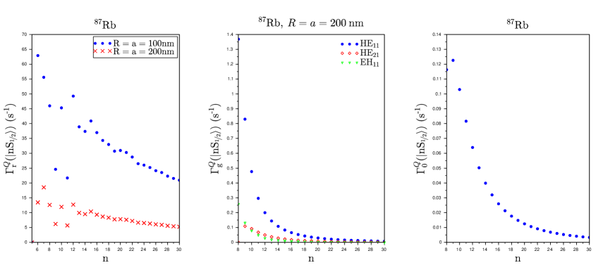
Figure 8: Spontaneous emission of an ${}^{87}\text{Rb}$ atom near an optical nanofiber – Contribution of the electric quadrupolar transitions. We represent the contribution of the electric quadrupolar transitions to the spontaneous emission rates into the radiative modes, $\Gamma_{r}^{Q}$ (left), the first guided modes, $\Gamma_{g}^{Q}$ (middle), and in vacuum, $\Gamma_{0}^{Q}$ (right), for an ${}^{87}\text{Rb}$ atom in the state $\left|nS_{\nicefrac{{1}}{{2}}}\right\rangle$ as a function of the principal quantum number, $n$. To get the highest possible value, we assume the atom is located on the nanofiber surface, i.e., $R=a$. In the case of the radiative modes (left), we considered two values for the fiber radius $a=100$ and $200$ nm, while $a=200$ nm for the other two plots.

III.1.4 Influence of the quantization axis

Until now, the quantization axis was implicitly fixed along the fiber axis $\left(Oz\right)$. Here, in the spirit of the experimental work in Ref (SGX19, ), we study how the spontaneous emission rate of an atom close to an optical nanofiber depends on the direction of the quantization axis chosen to define its state, and therefore the direction of its angular momentum polarization. The angles $\left(\Theta,\Phi\right)$ characterizing the quantization axis are specified in Fig. 9.

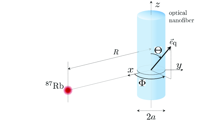
Figure 9: Definition of the angles $\left(\Theta,\Phi\right)$ characterizing the quantization axis directed along the unitary vector $\vec{e}_{\text{q}}\equiv\sin\Theta\cos\Phi\vec{e}_{x}+\sin\Theta\sin\Phi\vec{e}_{y}+\cos\Theta\vec{e}_{z}$.

To be more specific, Figs. 10, 11 and 12 show the variations of the spontaneous emission rates towards the first four guided modes, $\Gamma_{g}$ (left), and towards the radiative modes, $\Gamma_{r}$ (right), for an ${}^{87}\text{Rb}$ atom prepared in the state $\left|30D_{\nicefrac{{5}}{{2}}},F=4,M_{F}=4\right\rangle$ and located at a distance $R=300$ nm from the axis of a silica optical nanofiber of radius $a=250$ nm when the quantization axis rotates in the planes $\left(Oxy\right)$, $\left(Oxz\right)$ and $\left(Oyz\right)$, respectively.

Guided modes

Before discussing our results on $\Gamma_{g}$ let us make a few remarks :

A. Owing to our choice of initial atom state, $\left|30D_{\nicefrac{{5}}{{2}}},F=4,M_{F}=4\right\rangle$, and the value of fiber radius considered here, $a=250\text{ nm}$, the only transitions along which the atom can decay by emitting a photon into a guided mode are $\sigma^{+}$-transitions towards $P$ states, whose dipole is contained in the plane orthogonal to the quantization axis.

B. A guided mode is characterized by its type (K=TE, TM, HE, EH), its frequency $\omega$, two integers $l\geq 0$ and $m\geq 0$ called the azimuthal and radial mode orders, respectively, and two numbers $f=\pm 1$ and $p=\pm 1$, which characterize the propagation direction of the mode ($f=\pm 1$ conventionally corresponds to a mode propagating along $\left(Oz\right)$ towards increasing/decreasing $z$) and the counterclockwise or clockwise phase circulation of the mode, respectively (KBT17, ).

C. Because of field confinement, a guided mode $\mu\equiv\left(\text{K}_{lm},\omega,f,p\right)$ possesses a non-vanishing longitudinal component, $E_{z}^{\left(\mu\right)}$ (except for K=TE) (KR14, ). For the guided modes considered, $E_{z}^{\left(\mu\right)}$ and $E_{y}^{\left(\mu\right)}$can be chosen as real and $E_{x}^{\left(\mu\right)}$ is then purely imaginary. Moreover, the mode field components can be written in the form

$$E_{x}^{\left(\mu\right)} = \text{i}\mathcal{E}_{x}^{\left(\text{K}_{lm},\omega\right)}$$

$$E_{y}^{\left(\mu\right)} = p\mathcal{E}_{y}^{\left(\text{K}_{lm},\omega\right)}$$

$$E_{z}^{\left(\mu\right)} = f\mathcal{E}_{z}^{\left(\text{K}_{lm},\omega\right)}$$

where $\mathcal{E}_{x,y,z}^{\left(\text{K}_{lm},\omega\right)}$ are real functions of space and time, independent of $f$ and $p$.

D. Finally, note that $\mathcal{E}_{x}^{\left(\text{TE}_{0m},\omega\right)}=\mathcal{E}_{z}^{\left(\text{TE}_{0m},\omega\right)}=0$ and $\mathcal{E}_{y}^{\left(\text{TM}_{0m},\omega\right)}=0$.

Figure 10 corresponds to the configuration $\Theta\equiv\frac{\pi}{2}$, i.e., the quantization axis is chosen in the plane $\left(Oxy\right)$ and directed along the vector $\vec{e}_{\text{q}}\equiv\cos\Phi\vec{e}_{x}+\sin\Phi\vec{e}_{y}$. The dipole, $\vec{d}_{kn}$, associated with the $\sigma^{+}$-de-excitation, $\left|n\right\rangle\rightarrow\left|k\right\rangle$, of frequency $\omega_{nk}$, can, therefore, be written in the form $\vec{d}_{kn}=\frac{d_{kn}}{\sqrt{2}}\left[\text{i}\left(\sin\Phi\vec{e}_{x}-\cos\Phi\vec{e}_{y}\right)+\vec{e}_{z}\right]$. According to the remarks above, the coupling factor $\vec{d}_{kn}\cdot\vec{E}^{\left(\mu\right)}$ of a given transition $\left|n\right\rangle\rightarrow\left|k\right\rangle$ to the (resonant) guided mode $\mu\equiv\left(\text{K}_{lm},\omega_{nk},f,p\right)$ is proportional to $f\mathcal{E}_{z}^{\left(\text{K}_{lm},\omega_{nk}\right)}-\mathcal{E}_{x}^{\left(\text{K}_{lm},\omega_{nk}\right)}\sin\Phi-\text{i}p\mathcal{E}_{y}^{\left(\text{K}_{lm},\omega_{nk}\right)}\cos\Phi$ and the associated contribution to the spontaneous emission rate is, therefore, itself proportional to $\left(f\mathcal{E}_{z}^{\left(\text{K}_{lm},\omega_{nk}\right)}-\mathcal{E}_{x}^{\left(\text{K}_{lm},\omega_{nk}\right)}\sin\Phi\right)^{2}+\left(\mathcal{E}_{y}^{\left(\text{K}_{lm},\omega_{nk}\right)}\right)^{2}\cos^{2}\Phi$. Summing over $f=\pm 1$, $p=\pm 1$ and all possible final states, $\left|k\right\rangle$, we conclude that the spontaneous emission rate, $\Gamma_{g}^{\left(\text{K}_{lm}\right)}$, into the first four guided modes $\text{K}_{lm}=\text{HE}_{11}$, $\text{TE}_{01}$, $\text{TM}_{01}$ and $\text{HE}_{21}$, is proportional to

$$\sum_{k}\left\{\left(\mathcal{E}_{z}^{\left(\text{K}_{lm},\omega_{nk}\right)}\right)^{2}+\left(\mathcal{E}_{x}^{\left(\text{K}_{lm},\omega_{nk}\right)}\right)^{2}\sin^{2}\Phi+\left(\mathcal{E}_{y}^{\left(\text{K}_{lm},\omega_{nk}\right)}\right)^{2}\cos^{2}\Phi\right\}$$

(Note that cross-terms between $E_{z}$ and $E_{x}$ compensate each other when summing over $f$). In agreement with Fig. 10, we conclude that: i) $\Gamma_{g}^{\left(\text{K}_{lm}\right)}$ is a $\pi$-periodic function of $\Phi$ and reaches its extrema when $\Phi=0\left[\frac{\pi}{2}\right]$. ii) For the modes $\text{TE}_{01}$, since $\mathcal{E}_{x}=\mathcal{E}_{z}=0$, $\Gamma_{g}^{\left(\text{TE}_{01}\right)}\left(\Phi\right)\propto\cos^{2}\Phi$ is maximal for $\Phi=0\left[\pi\right]$, minimal for $\Phi=\frac{\pi}{2}\left[\pi\right]$ and its minimum is zero. iii) For the modes $\text{TM}_{01}$, since $\mathcal{E}_{y}=0$, $\Gamma_{g}^{\left(\text{TM}_{01}\right)}\left(\Phi\right)\propto\sum_{k}\left\{\left(\mathcal{E}_{z}^{\left(\text{TM}_{01},\omega_{nk}\right)}\right)^{2}+\left(\mathcal{E}_{x}^{\left(\text{TM}_{01},\omega_{nk}\right)}\right)^{2}\sin^{2}\Phi\right\}$ is maximal for $\Phi=\frac{\pi}{2}\left[\pi\right]$, minimal for $\Phi=0\left[\pi\right]$ and its minimum is different from zero. For other modes $\left(\text{K}_{lm}=\text{HE}_{11},\text{HE}_{21}\right)$, Fig. 10 shows that minima and maxima of $\Gamma_{g}^{\left(\text{K}_{lm}\right)}\left(\Phi\right)$ are also reached for $\Phi=0\left[\pi\right]$ and $\Phi=\frac{\pi}{2}\left[\pi\right]$, respectively. This can be explained by the inequality $\left|\mathcal{E}_{x}\right|\geq\left|\mathcal{E}_{y}\right|$ valid for these modes and the values $\left(a,R\right)$ considered.

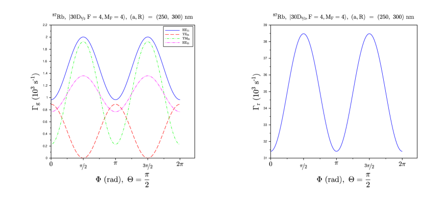
Figure 10: Spontaneous emission of an ${}^{87}\text{Rb}$ atom near an optical nanofiber with quantization axis in the $\left(Oxy\right)$ plane. We plot the spontaneous emission rates, $\Gamma_{g}$ (left) and $\Gamma_{r}$ (right), into the first guided and radiative modes, respectively, for an ${}^{87}\text{Rb}$ atom in the state $\left|30D_{\nicefrac{{5}}{{2}}},F=4,M_{F}=4\right\rangle$ as functions of the angle $\Phi$ (c.f. Fig. 9), with $\Theta=\nicefrac{{\pi}}{{2}}$. The contributions to $\Gamma_{g}$ of the first four guided modes, $\text{HE}_{11},\text{TE}_{01}$, $\text{TM}_{01}$ and $\text{HE}_{21}$, are displayed separately. The radius of the fiber is $a=250$ nm and the atom is located $50$ nm from the fiber (i.e., $R=a+50$ nm).

The same arguments can be used to interpret Fig. 11. This time, the quantization axis is chosen in the plane $\left(Oxz\right)$, i.e., $\Phi\equiv 0$, and $\vec{e}_{\text{q}}\equiv\sin\Theta\vec{e}_{x}+\cos\Theta\vec{e}_{z}$, whence $\vec{d}_{kn}=\frac{d_{kn}}{\sqrt{2}}\left[\text{i}\left(\sin\Theta\vec{e}_{z}-\cos\Theta\vec{e}_{x}\right)+\vec{e}_{y}\right]$. The contribution to the spontaneous emission rate into the resonant guided mode $\mu\equiv\left(\text{K}_{lm},\omega_{nk},f,p\right)$ of a given transition $\left|n\right\rangle\rightarrow\left|k\right\rangle$ is proportional to $\left(\cos\Theta\mathcal{E}_{x}^{\left(\text{K}_{lm},\omega_{nk}\right)}+p\mathcal{E}_{y}^{\left(\text{K}_{lm},\omega_{nk}\right)}\right)^{2}+\left(\mathcal{E}_{z}^{\left(\text{K}_{lm},\omega_{nk}\right)}\right)^{2}\sin^{2}\Theta$. Summing over $f=\pm 1$, $p=\pm 1$, and $k$, we conclude that the spontaneous emission rate $\Gamma_{g}^{\left(\text{K}_{lm}\right)}$ into guided modes $\text{K}_{lm}=\text{HE}_{11}$, $\text{TE}_{01}$, $\text{TM}_{01}$ or $\text{HE}_{21}$, is proportional to

$$\sum_{k<n}\left\{\cos^{2}\Theta\left(\mathcal{E}_{x}^{\left(\text{K}_{lm},\omega_{nk}\right)}\right)^{2}+\left(\mathcal{E}_{y}^{\left(\text{K}_{lm},\omega_{nk}\right)}\right)^{2}+\left(\mathcal{E}_{z}^{\left(\text{K}_{lm},\omega_{nk}\right)}\right)^{2}\sin^{2}\Theta\right\}$$

(Note that cross-terms between $E_{x}$ and $E_{y}$ now compensate each other when summing over $p$). In agreement with Fig. 11, we conclude that : i) $\Gamma_{g}^{\left(\text{K}_{lm}\right)}$ is a $\pi$-periodic function of $\Theta$ which reaches its extrema for $\Theta=0\left[\frac{\pi}{2}\right]$. ii) For the modes $\text{TE}_{01}$, since $\mathcal{E}_{x}=\mathcal{E}_{z}=0$, $\Gamma_{g}^{\left(\text{TE}_{01}\right)}\left(\Theta\right)$ is constant. iii) For other modes $\left(\text{K}_{lm}=\text{HE}_{11},\text{TM}_{01},\text{HE}_{21}\right)$, Fig. 11 shows that maxima and minima are achieved for $\Theta=0\left[\pi\right]$ and $\Theta=\frac{\pi}{2}\left[\pi\right]$, respectively, i.e., $\Gamma_{g,\text{max}}\propto\sum_{\alpha}\left\{\left(\mathcal{E}_{x}^{\left(\text{K}_{lm},\omega_{nk}\right)}\right)^{2}+\left(\mathcal{E}_{y}^{\left(\text{K}_{lm},\omega_{nk}\right)}\right)^{2}\right\}$ and $\Gamma_{g,\text{min}}\propto\sum_{\alpha}\left\{\left(\mathcal{E}_{y}^{\left(\text{K}_{lm},\omega_{nk}\right)}\right)^{2}+\left(\mathcal{E}_{z}^{\left(\text{K}_{lm},\omega_{nk}\right)}\right)^{2}\right\}$. This can be explained by the inequality $\left|\mathcal{E}_{x}\right|\geq\left|\mathcal{E}_{z}\right|$ valid for these modes and the values $\left(a,R\right)$ considered.

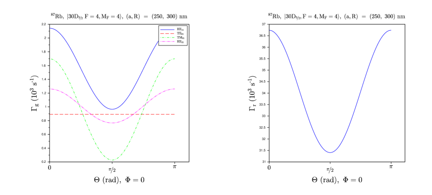
Figure 11: Spontaneous emission of an ${}^{87}\text{Rb}$ atom near an optical nanofiber with quantization axis in the $\left(Oxz\right)$ plane. We represent the spontaneous emission rates, $\Gamma_{g}$ (left) and $\Gamma_{r}$ (right), into the first guided and radiative modes, respectively, for an ${}^{87}\text{Rb}$ atom in the state $\left|30D_{\nicefrac{{5}}{{2}}},F=4,M_{F}=4\right\rangle$ as functions of the angle $\Theta$ (c.f. Fig. 9), with $\Theta=\nicefrac{{\pi}}{{2}}$. The contributions to $\Gamma_{g}$ of the first four guided modes, $\text{HE}_{11},\text{TE}_{01}$, $\text{TM}_{01}$ and $\text{HE}_{21}$ are displayed separately. The radius of the fiber is $a=250$ nm and the atom is located $50$ nm from the fiber (i.e., $R=a+50$ nm).

Finally, in Fig. 12, the quantization axis is chosen in the plane $\left(Oyz\right)$, i.e. $\Phi\equiv\nicefrac{{\pi}}{{2}}$, and $\vec{e}_{\text{q}}\equiv\sin\Theta\vec{e}_{y}+\cos\Theta\vec{e}_{z}$, whence $\vec{d}_{kn}=\frac{d_{kn}}{\sqrt{2}}\left[\text{i}\left(\cos\Theta\vec{e}_{y}-\sin\Theta\vec{e}_{z}\right)+\vec{e}_{x}\right]$. The contribution to the spontaneous emission rate into the resonant guided mode $\mu\equiv\left(\text{K}_{lm},\omega_{nk},f,p\right)$ of a given transition $\left|n\right\rangle\rightarrow\left|k\right\rangle$ is proportional to $\left[\mathcal{E}_{x}^{\left(\text{K}_{lm},\omega_{nk}\right)}+\cos\Theta p\mathcal{E}_{y}^{\left(\text{K}_{lm},\omega_{nk}\right)}-\sin\Theta f\mathcal{E}_{z}^{\left(\text{K}_{lm},\omega_{nk}\right)}\right]^{2}$. Summing over $f=\pm 1$, $p=\pm 1$, and $k$, we conclude that the spontaneous emission rate, $\Gamma_{g}^{\left(\text{K}_{lm}\right)}$, into guided modes of type $\text{K}_{lm}=\text{HE}_{11}$, $\text{TE}_{01}$, $\text{TM}_{01}$ and $\text{HE}_{21}$ is proportional to

$$\sum_{k<n}\left\{\left(\mathcal{E}_{x}^{\left(\text{K}_{lm},\omega_{nk}\right)}\right)^{2}+\cos^{2}\Theta\left(\mathcal{E}_{y}^{\left(\text{K}_{lm},\omega_{nk}\right)}\right)^{2}+\sin^{2}\Theta\left(\mathcal{E}_{z}^{\left(\text{K}_{lm},\omega_{nk}\right)}\right)^{2}\right\}$$

(Note that cross-terms between $E_{x}$, $E_{y}$ and $E_{z}$ now compensate each other when summing over $p$ and $f$). In agreement with Fig. 12, we conclude that : i) $\Gamma_{g}^{\left(\text{K}_{lm}\right)}$ is a $\pi$-periodic function of $\Theta$ which reaches its extrema in $\Theta=0\left[\frac{\pi}{2}\right]$. ii) For the modes $\text{TE}_{01}$, since $\mathcal{E}_{x}=\mathcal{E}_{z}=0$, $\Gamma_{g}^{\left(\text{TE}_{01}\right)}\left(\Theta\right)\propto\cos^{2}\Theta$ is maximal for $\Theta=0\left[\pi\right]$, minimal for $\Theta=\frac{\pi}{2}\left[\pi\right]$ and its minimum is zero. According to Fig. 12, $\Gamma_{g}^{\left(\text{HE}_{11}\right)}\left(\Theta\right)$ also reaches its maxima and minima in $\Theta=0\left[\pi\right]$ and $\Theta=\frac{\pi}{2}\left[\pi\right]$, respectively. This can be explained by the inequality $\left|\mathcal{E}_{y}^{\text{HE}_{11}}\right|\geq\left|\mathcal{E}_{z}^{\text{HE}_{11}}\right|$ valid for the values $\left(a,R\right)$ considered. iii) For the modes $\text{TM}_{01}$, since $\mathcal{E}_{y}=0$, $\Gamma_{g}^{\left(\text{TM}_{01}\right)}\left(\Theta\right)\propto\sum_{k<n}\left\{\left(\mathcal{E}_{x}^{\left(\text{TM}_{01},\omega_{nk}\right)}\right)^{2}+\sin^{2}\Theta\left(\mathcal{E}_{z}^{\left(\text{TM}_{01},\omega_{nk}\right)}\right)^{2}\right\}$ is maximal for $\Theta=\frac{\pi}{2}\left[\pi\right]$, minimal for $\Theta=0\left[\pi\right]$. According to Fig. 12, $\Gamma_{g}^{\left(\text{HE}_{21}\right)}\left(\Theta\right)$ also reaches its maxima and minima in $\Theta=\frac{\pi}{2}\left[\pi\right]$ and $\Theta=0\left[\pi\right]$, respectively. This can be explained by the inequality $\left|\mathcal{E}_{z}\right|\geq\left|\mathcal{E}_{y}\right|$ valid for $\text{HE}_{21}$ modes and the values $\left(a,R\right)$ considered.

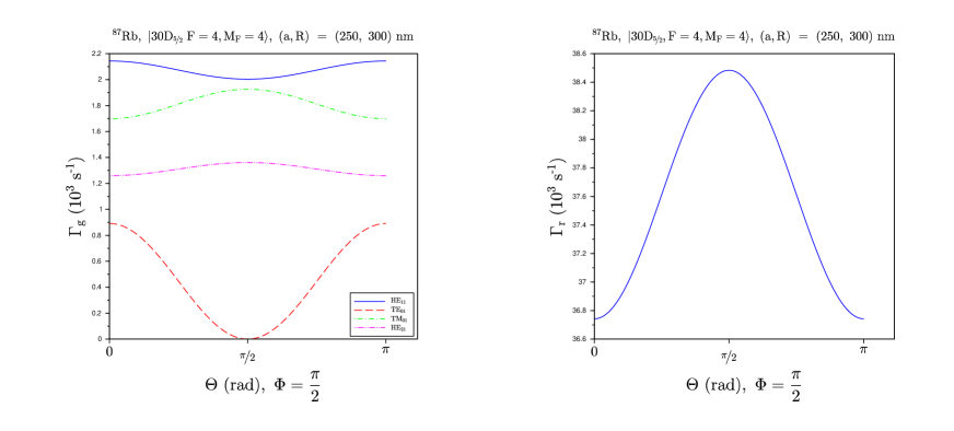
Figure 12: Spontaneous emission of an ${}^{87}\text{Rb}$ atom near an optical nanofiber with quantization axis in the $\left(Oyz\right)$ plane. We represent the spontaneous emission rates, $\Gamma_{g}$ (left) and $\Gamma_{r}$ (right), into the first guided and radiative modes, respectively, for an ${}^{87}\text{Rb}$ atom in the state $\left|30D_{\nicefrac{{5}}{{2}}},F=4,M_{F}=4\right\rangle$ as functions of the angle $\Theta$ (c.f. Fig. 9), with $\Phi=\nicefrac{{\pi}}{{2}}$. The contributions to $\Gamma_{g}$ of the first three guided modes, $\text{HE}_{11},\text{TE}_{01}$ and $\text{TM}_{01}$, are displayed separately. The radius of the fiber is $a=250$ nm (i.e. $R=a+50$ nm).

Radiative modes

Our results on the spontaneous emission rate into the radiative modes are displayed in the right-hand panels of Figs. 10, 11 and 12. In the three different configurations, one observes a $\pi$-periodicity in $\left(\Phi,\Theta\right)$. Moreover, the three figures seem to indicate that, for the values of $\left(a,R\right)$ considered, radiative modes contributing to $\Gamma_{r}$ are mainly radial, i.e., their component along $\left(Ox\right)$ dominates. Due to the variety and complexity of the structure of radiative modes, it is, however, difficult to go further into the interpretation of our results.

Proportion of spontaneously emitted light towards the guided modes

Figure 13 displays a 3D “summary” of Figs. 10, 11 and 12. To be more explicit, it shows the ratio $\nicefrac{{\Gamma_{g}}}{{\Gamma}}$ characterizing the proportion of spontaneous emitted light captured by guided modes. Note that the contribution of $\text{HE}_{11}$ to $\Gamma_{g}$ dominates. Besides $\pi$-periodicity in $\Phi$ and $\Theta$, one observes maxima for $\nicefrac{{\Gamma_{g}}}{{\Gamma}}$ for $\vec{e}_{\text{q}}=\vec{e}_{z}$ and saddle points for $\vec{e}_{\text{q}}=\vec{e}_{y}$.

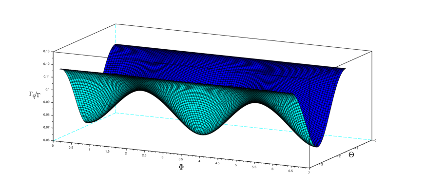
Figure 13: Spontaneous emission of an ${}^{87}\text{Rb}$ atom near an optical nanofiber. We represent the proportion of spontaneous emission into the guided modes, $\nicefrac{{\Gamma_{g}}}{{\Gamma}}$, for an ${}^{87}\text{Rb}$ atom in the state $|\mathrm{30D}_{5/2},F=4,M_{F}|=4\rangle$ as a function of the angles $\left(\Theta,\Phi\right)$ (c.f. Fig. 9).

III.1.5 Anisotropic spontaneous emission

Througout this section, the quantization axis is chosen along $\left(Oy\right)$. Using the same notations as in the previous section, this corresponds to $\vec{e}_{\text{q}}=\vec{e}_{y}$. In this configuration, the atomic dipole associated with, e.g., a $\sigma^{+}$-transition $\left|n\right\rangle\rightarrow\left|k\right\rangle$ lies in the plane $\left(Oxz\right)$ and, more explicitly, $\vec{d}_{kn}=\frac{d_{kn}}{\sqrt{2}}\left[\text{i}\vec{e}_{x}+\vec{e}_{z}\right]$. Using, as in the previous section, the simplistic mode function approach, we conclude that the contribution of this transition to the spontaneous emission rate into a specific guided mode $\mu=\left(\text{K}_{lm},\omega_{nk},f,p\right)$ is proportional to $\left(f\mathcal{E}_{z}^{\left(K_{lm},\omega_{nk}\right)}-\mathcal{E}_{x}^{\left(K_{lm},\omega_{nk}\right)}\right)^{2}$ and clearly depends on the propagation direction, $f$. This heuristic argument cannot be straightforwardly transposed to radiative modes, but the same phenomenon is observed. The anisotropic spontaneous emission leads to a non-vanishing average lateral force on the atom whose order of magnitude is $0.5$ zN (5 zN) for a rubidium atom in a $5D$ $\left(5P\right)$ state located at a distance $d=50$ nm from a fiber of radius $a=200$ nm. This force corresponds to the resonant part of the average Lorentz force, $\left[F^{\text{res}}\right]_{z}$, Eq. (5) (Buh12, ), and can be calculated in the Green’s function approach. In particular, for an atom initially in a state $\left|n\right\rangle$, one can decompose $\left[F^{\text{res}}\right]_{z}$ as the sum of contributions $\left[F_{nk,\nu}^{\text{res}}\right]_{z}$ relative to the transition $\left|n\right\rangle\rightarrow\left|k\right\rangle$ coupled to the (guided or radiative) mode, $\nu$.

In order to quantitatively characterize the anisotropy of emission, we introduce the factor

$$\alpha_{n}\equiv\sum_{\nu,k<n}\frac{\Gamma_{nk,\nu}}{\Gamma_{n}}\times\frac{\hbar k_{\nu,z}}{\hbar k_{\nu}}$$

where the sum runs over all (radiative and guided) modes, $\nu$, and final states, $k$. In this expression, $\Gamma_{nk,\nu}$ represents the spontaneous emission rate for the transition $\left|n\right\rangle\rightarrow\left|k\right\rangle$ into the mode $\nu$, $\Gamma_{n}$ is the total spontaneous emission rate from the state $\left|n\right\rangle$, $k_{\nu,z}$ is the projection onto $\left(Oz\right)$ of the wavevector for the (guided or radiative) mode $\left(\nu\right)$ and $k_{\nu}=\nicefrac{{\omega_{\nu}}}{{c}}$ is its norm. With these definitions, $\left(\nicefrac{{\Gamma_{nk,\nu}}}{{\Gamma_{n}}}\right)$ can be interpreted as the probability for a photon to be emitted from the state $\left|n\right\rangle$ via the transition $\left|n\right\rangle\rightarrow\left|k\right\rangle$ and into the mode $\nu$, while $\nicefrac{{\hbar k_{\nu,z}}}{{\hbar k_{\nu}}}$ characterizes the inclination of the momentum of the photon emitted into the mode $\nu$ with respect to the fiber axis.

Identifying $-\hbar k_{\nu,z}\Gamma_{nk,\nu}$, i.e., the atomic recoil along $\left(Oz\right)$ induced by the emission of a photon into the mode, $\nu$, via the transition $\left|n\right\rangle\rightarrow\left|k\right\rangle$, with the force $\left[F_{nk,\nu}^{\text{res}}\right]_{z}$, one can write $\alpha_{n}=-\sum_{k,\nu}\nicefrac{{\left[F_{nk,\nu}^{\text{res}}\right]_{z}}}{{\Gamma_{n}\hbar k_{\nu}}}$ (see (SBC15, ) and Appendix B). Figs. 14 and 15 show the coefficient $\alpha_{n}$ for an ${}^{87}\text{Rb}$ atom prepared in an excited $S,P$ or $D$ state decaying via $\sigma^{+}$-transitions located close to an optical nanofiber of radius $a=200$ nm as a function of the distance $R$ from the atom to the fiber axis, $Oz$. The observed Drexhage-like oscillations are due to radiative modes (D70, ). Remarkably, though very weak, the spontaneous emission anisotropy for the $S$ states is nonzero, at around $0.4\%$ at most (see Fig. 14). For $S$ states, $\alpha$ decreases for increasing $n$ and vanishes when $R\rightarrow+\infty$ as expected (equivalent to the free-space configuration). As seen in Fig. 15, for $P$ and $D$ states, the spontaneous emission anisotropy, at around $20\%$ on the surface of the nanofiber, is much stronger than for $S$ states. When $R\rightarrow+\infty$, $\alpha_{n}$ tends to zero as expected. For $P$ states, $\alpha_{n}$ decreases with $n$, while it only slightly varies for $D$ states. Anisotropic emission is, therefore, observable for $D$ states even at high values of $n$.

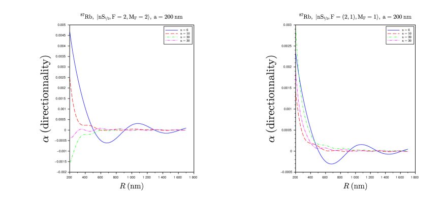
Figure 14: Directionality of the spontaneous emission of an ${}^{87}\text{Rb}$ atom near an optical nanofiber. We represent the coefficient, $\alpha_{n}$ (see main text for definition), characterizing the directionality of the spontaneous emission with respect to the $z$-axis, of an ${}^{87}\text{Rb}$ atom in the states $|\mathrm{nS}_{1/2},F=2,M_{F}=2\rangle$ (left panel) and $|\mathrm{nS}_{1/2},F=\left(2,1\right),M_{F}=1\rangle$ (right panel) for $n=6,10,20,30$, close to an optical nanofiber of radius $a=200$ nm as a function of the distance, $R$, from the atom to the fiber axis.

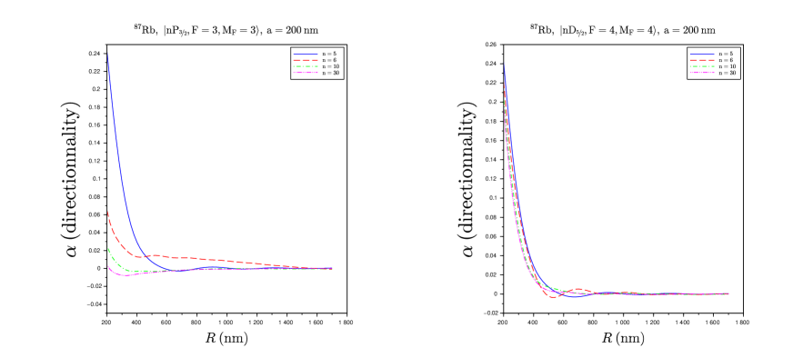
Figure 15: Directionality of the spontaneous emission of an ${}^{87}\text{Rb}$ atom near an optical nanofiber – We represent the coefficient, $\alpha_{n}$ (see main text for definition), characterizing the directionality with respect to the $z$ axis, of the spontaneous emission of an ${}^{87}\text{Rb}$ atom in the states $|\mathrm{nP}_{3/2},F=3,M_{F}=3\rangle$ (left panel) and $|\mathrm{nD}_{5/2},F=4,M_{F}=4\rangle$ (right panel) for $n=5,6,10,30$, close to an optical nanofiber of radius $a=200$ nm as a function of the distance, $R$, from the atom to the fiber axis.

Anisotropic spontaneous emission into the guided modes of the nanofiber

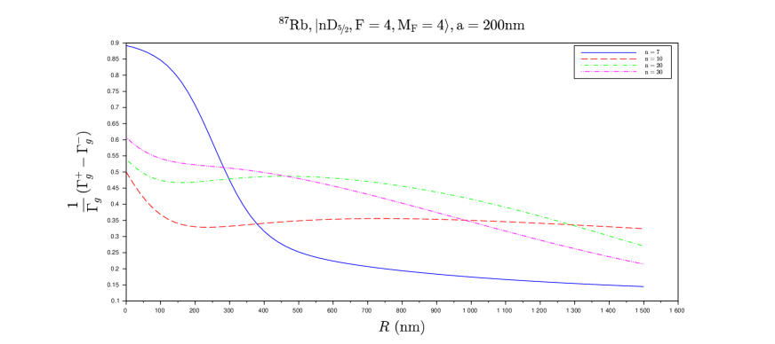
Figure 16: Directionality of the spontaneous emission of an ${}^{87}\text{Rb}$ atom near an optical nanofiber into the guided modes – We represent the ratio, $\nicefrac{{\left(\Gamma_{g}^{\left(+\right)}-\Gamma_{g}^{\left(-\right)}\right)}}{{\Gamma_{g}}}$ (see main text for definitions), characterizing the directionality with respect to the $z$ axis, of the spontaneous emission into the guided modes of an ${}^{87}\text{Rb}$ atom in the state $|\mathrm{nD}_{5/2},F=4,M_{F}=4\rangle$ for $n=7,10,20,30$, close to an optical nanofiber of radius $a=200$ nm as a function of the distance, $R$, from the atom to the fiber axis.

For guided modes, the anisotropy can be further characterized by the ratio, $\nicefrac{{\left(\Gamma_{g}^{\left(+\right)}-\Gamma_{g}^{\left(-\right)}\right)}}{{\Gamma_{g}}}$, where $\Gamma_{g}^{\left(\pm\right)}$ denotes the spontaneous emission rate into forward/backward propagating guided modes and $\Gamma_{g}\equiv\Gamma_{g}^{+}+\Gamma_{g}^{-}$. Using the same arguments as above, one can write this factor in the following form: $-\sum_{k,\mu}\nicefrac{{\left[F_{nk,\mu}^{\text{res}}\right]_{z}}}{{\Gamma_{g}\hbar\left|k_{\mu,z}\right|}}$, where now the sum runs over the guided modes, $\mu$, only (see (KR14, ) and Appendix B). Figure 16 shows the ratio $\nicefrac{{\left(\Gamma_{g}^{\left(+\right)}-\Gamma_{g}^{\left(-\right)}\right)}}{{\Gamma_{g}}}$ calculated for an ${}^{87}\text{Rb}$ atom prepared in the state $|\mathrm{nD}_{5/2},F=4,M_{F}=4\rangle$, with $n=7,10,20,30$, and located near an optical nanofiber of radius $a=200$ nm, as a function of the distance, $R$, from the atom to the fiber axis. The directionality of the guided emitted light remains strong even for high values of $n$ and $R$. Note, however, that for large $R>300$ nm the absolute value of $\Gamma_{g}$ itself is so small that the directionality has little practical meaning.

III.2 Lamb shift and van der Waals force

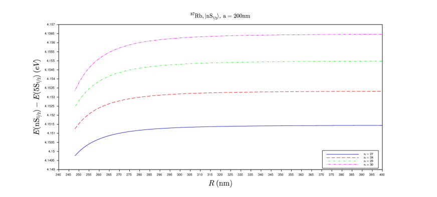
Figure 17: Lamb shift of an ${}^{87}\text{Rb}$ atom in the state $\left|nS_{\nicefrac{{1}}{{2}}}\right\rangle$, for $n=27,\cdots,30$ near an optical nanofiber – We represent the energy difference, $E\left(nS_{\nicefrac{{1}}{{2}}}\right)-E\left(5S_{\nicefrac{{1}}{{2}}}\right)$, of the states $\left|nS_{\nicefrac{{1}}{{2}}}\right\rangle$ ($n=27\cdots 30$) and $\left|5S_{\nicefrac{{1}}{{2}}}\right\rangle$ of an ${}^{87}\text{Rb}$ atom near an optical nanofiber of radius, $a=200$ nm as a function of the distance, $R$, from the fiber. Energies are given in eV.

Figure 17 displays the energy difference, $E\left(nS_{\nicefrac{{1}}{{2}}}\right)-E\left(5S_{\nicefrac{{1}}{{2}}}\right)$, of the states $\left|nS_{\nicefrac{{1}}{{2}}}\right\rangle$ ($n=27\cdots 30$) and $\left|5S_{\nicefrac{{1}}{{2}}}\right\rangle$ for an ${}^{87}\text{Rb}$ atom near an optical nanofiber of radius $a=200$ nm as a function of the distance, $R$, from the fiber axis. The Lamb shift of the ground state is assumed to be negligible with respect to that of the excited levels. When $R$ decreases, $\left[E\left(nS_{\nicefrac{{1}}{{2}}}\right)-E\left(5S_{\nicefrac{{1}}{{2}}}\right)\right]$ itself decreases, though more rapidly for higher $n$. At shorter distances from the fiber, energy curves cross (not shown on Fig. 17) and the perturbative approach fails. The treatment of this area requires the diagonalization of the full Hamiltonian in the relevant degenerate Hilbert subspace. This will be investigated in future work.

Figure 18 shows the same quantity for states $\left|nD_{\nicefrac{{5}}{{2}}}F=4,m_{F}=-F\cdots F\right\rangle$ and

$\left|nP_{\nicefrac{{3}}{{2}}}F=3,m_{F}=-F\cdots F\right\rangle$ for $n=29,30$. Though the order of magnitude is comparable to that obtained for states $\left|nS_{\nicefrac{{1}}{{2}}}\right\rangle$, one observes a degeneracy lift of the hyperfine components of different $\left|M_{F}\right|$ very close to the fiber; to be more explicit, the Lamb shift is stronger for states of higher $\left|M_{F}\right|$. This can be qualitatively justified as follows: i) Radiative and guided modes have a strong – though not exclusive – transverse component, i.e., orthogonal to the fiber axis $\left(Oz\right)$ (see Fig. 1); ii) High coupling to the guided modes is, therefore, obtained for transitions corresponding to dipoles in the transverse plane, $\left(Oxy\right)$; iii) The quantization axis being along the fiber axis, dipoles in the plane $\left(Oxy\right)$ correspond to $\sigma$ transitions: therefore, the stronger the weight of $\sigma$ transitions in the de-excitation of an excited state, the higher the spontaneous emission rate into guided modes; iv) The higher $\left|M_{F}\right|$, the stronger the weight of $\sigma$ transitions in the de-excitation of the state (this can be directly checked on $3j$-coefficients): therefore, the higher $\left|M_{F}\right|$, the higher the spontaneous emission rate into guided modes.

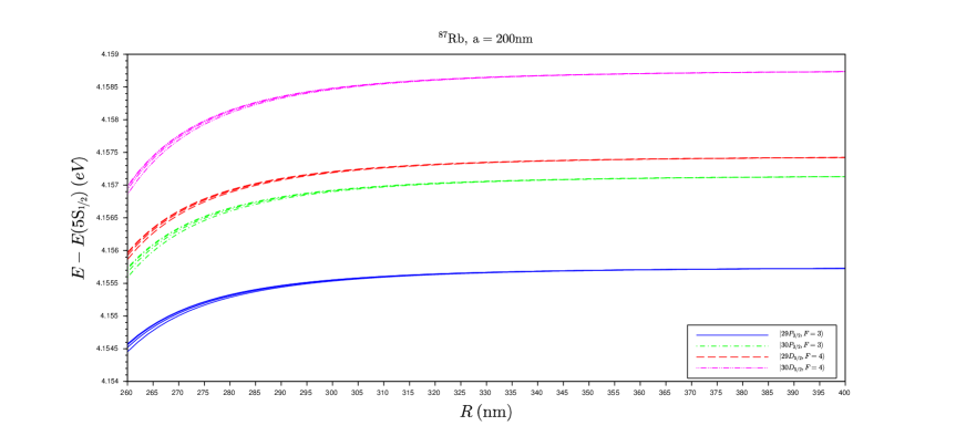
Figure 18: Lamb shift of an ${}^{87}\text{Rb}$ atom in the states $\left|nP_{\nicefrac{{3}}{{2}}}F=3,M_{F}=-F\cdots F\right\rangle$ and $\left|nD_{\nicefrac{{5}}{{2}}}F=4,M_{F}=-F\cdots F\right\rangle$, for $n=29,30$ near an optical nanofiber – We represent the energy difference, $E-E\left(5S_{\nicefrac{{1}}{{2}}}\right)$, of the states of interest with respect to $\left|5S_{\nicefrac{{1}}{{2}}}\right\rangle$ as a function of the distance, $R$, from the fiber. The radius of the nanofiber is $a=200$ nm. Energies are given in eV.

The $R$-dependence of the Lamb shift results in a radial van der Waals force, $-\partial_{R}U_{n}\left(R\right)$, represented in Fig. 19 for the state $\left|30S_{\nicefrac{{1}}{{2}}}\right\rangle$ as a function of $R$. Note the negative sign and, therefore, the attractive character of the force, as well as its order of magnitude of $10^{-14}\text{N}$, much larger than spontaneous emission recoil induced forces. Aside from the total force, we represented the contributions of the electric dipole and quadrupole couplings. Though the dipole contribution dominates, the quadrupolar component is far from negligible, especially close to the nanofiber when field inhomogeneities are magnified.

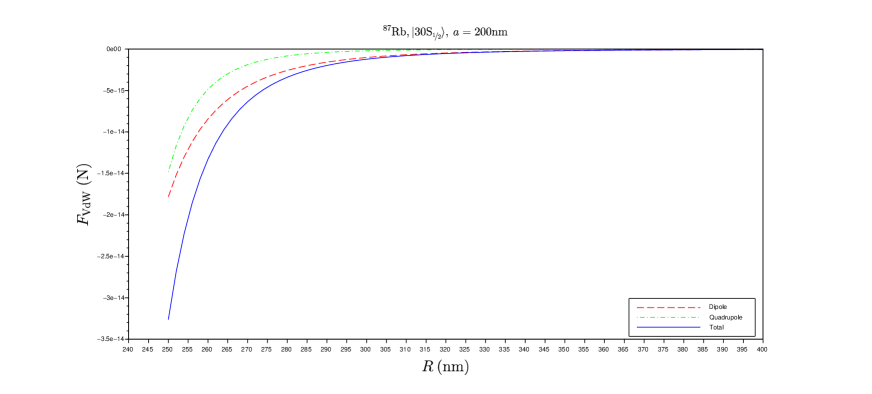
Figure 19: van der Waals force felt by an ${}^{87}\text{Rb}$ atom in the state $\left|30S_{\nicefrac{{1}}{{2}}}\right\rangle$, for $n=25,\cdots,30$ near an optical nanofiber – We represent the radial van der Waals force, $F_{vdW}=-\partial_{R}U\left(R\right)$, felt by an ${}^{87}\text{Rb}$ atom in the state $\left|30S_{\nicefrac{{1}}{{2}}}\right\rangle$ close to an optical nanofiber of radius $a=200$ nm as a function of the distance, $R$, from the fiber. The total force, electric dipole, and quadrupole coupling contributions are represented by (blue) full, (red) dashed, and (green) dashed-dotted lines, respectively.

Figure 20 displays the electric dipole and quadrupole components of the Lamb shift calculated for an ${}^{87}\text{Rb}$ atom in the state $\left|nS_{\nicefrac{{1}}{{2}}}\right\rangle$ located at a distance, $R=250$ nm from an optical nanofiber of radius $a=200$ nm. One observes that the higher the principal quantum number, $n$, the stronger the quadrupole component. For $n>35$, it even dominates the Lamb shift.

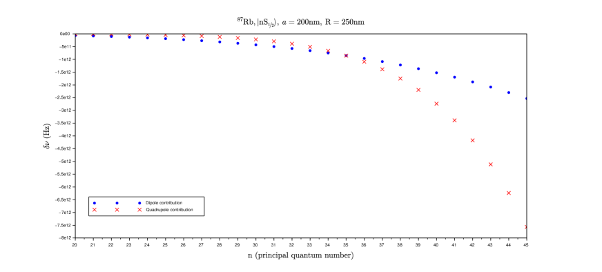
Figure 20: Electric dipole and quadrupole contributions to the Lamb shift of an ${}^{87}\text{Rb}$ atom in the state $\left|nS_{\nicefrac{{1}}{{2}}}\right\rangle$ near an optical nanofiber – Electric dipole and quadrupole components are represented as functions of the principal quantum number, $n$, by (blue) dots and (red) crosses, respectively. The radius of the optical nanofiber is $a=200$ nm and the atom is located at $R=250$ nm from the fiber axis.

One observes the same trend with $n$ in Fig. 21, which displays the relative contributions of the electric dipole and quadrupole couplings to the Lamb shift calculated for an ${}^{87}\text{Rb}$ atom in the state $\left|nS_{\nicefrac{{1}}{{2}}}\right\rangle$ located at four different distances $R=250,300,350,$ and $400$ nm from the optical nanofiber axis, as functions of $n$. As expected, the influence of quadrupolar transitions is lowered when the distance, $R$, increases, since the effect of the fiber on the electromagnetic field is less pronounced.

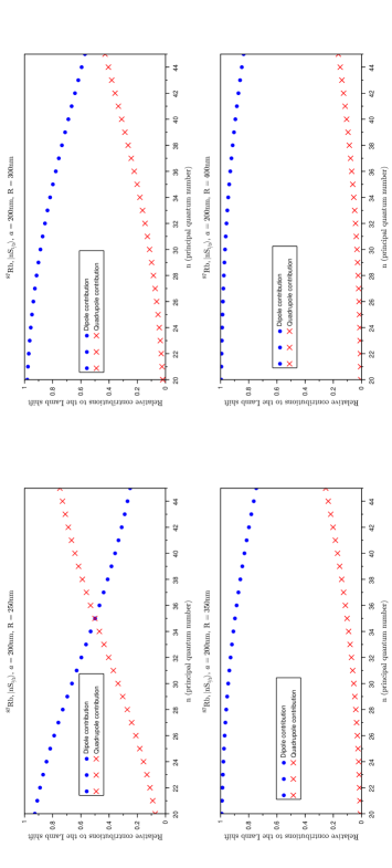
Figure 21: Relative contributions to the Lamb shift of electric dipole and quadrupole couplings for an ${}^{87}\text{Rb}$ atom in the state $\left|nS_{\nicefrac{{1}}{{2}}}\right\rangle$ close to an optical nanofiber – Electric dipole and quadrupole components are represented as functions of the principal quantum number, $n$, by (blue) dots and (red) crosses, respectively, for an atom located at $R=250\text{ (top left)},300\text{ (top right)},350\text{ (bottom left)}$ and $400$ nm (bottom right) from the fiber axis. The radius of the optical nanofiber is $a=200$ nm.

IV Conclusion

The influence of a nanofiber near an ${}^{87}\text{Rb}$ atom prepared in a Rydberg-excited state,

$\left|n\leq 30;L=S,P,D;JFM_{F}\right\rangle$, on the spontaneous emission rates and Lamb shift was investigated numerically in detail. In particular, the dependence of the spontaneous emission rates on the fiber radius, the distance of the atom to the fiber, the principal quantum number, $n$, orbital momentum, fine and hyperfine structures of the state considered, and the direction of angular momentum polarization were addressed. Close to the nanofiber, a non-negligible fraction of the emitted light can be captured by guided modes. This fraction is higher for larger $\left|M_{F}\right|$ but saturates for high $n$. When the quantum and fiber axes do not coincide, spontaneous emission into guided modes becomes strongly directional. This directionality persists even for high $n$. The contribution of quadrupolar transitions was shown to be negligible for spontaneous emission rates, while they may dominate Lamb shifts and van der Waals associated forces for high $n$. Our calculations were performed in the multimode fiber case, including all atomic transitions, using the general framework of macroscopic quantum electrodynamics and this allowed us to account for the dispersive and absorptive characteristics of silica.

Our work is a preliminary step towards the building of a Rydberg-atom-optical-nanofiber platform. In particular, the collection and guidance of a substantial part of the spontaneous emitted light along the nanofiber suggests the possibility of constructing a network of Rydberg atomic ensembles in the same spirit as described in (BCA12, ). The strong directionality of spontaneous emission observed for specific Rydberg states and quantization axis is also very promising in view of potential applications in chiral quantum information protocols (LMS17, ). In future works, we will address the case of several Rydberg atoms in the neighbourhood of an optical nanofiber. In particular, we shall be interested in studying how the nanofiber modifies the Rydberg blockade phenomenon and whether the geometric arrangement of atoms can be used to enhance the coupling to guided modes.

Appendix A Dyadic Green’s function for a cylindrical nanofiber

The dyadic Green’s function $\overline{\overline{G}}$ used throughout the main text is the solution of the Helmholtz equation

$$\left[\vec{\nabla}_{\vec{r}}\times\vec{\nabla}_{\vec{r}}\times-\varepsilon\left(\vec{r},\omega\right)\frac{\omega^{2}}{c^{2}}\right]\overline{\overline{G}}\left(\vec{r},\vec{r}^{\prime},\omega\right)=\delta\left(\vec{r}-\vec{r}^{\prime}\right)\overline{\overline{I}}$$ (7)

where the operator, $\vec{\nabla}_{\vec{r}}$, acts on the position vector, $\vec{r}$, $\overline{\overline{I}}$ is the unit dyadic, and $\varepsilon=\varepsilon_{1}\left(\omega\right)$ (silica relative electric permittivity) inside the nanofiber and $\varepsilon=1$ outside. As shown in (Tai94, ), $\overline{\overline{G}}$ splits into a vacuum term, $\overline{\overline{G}}_{0}$, which is the solution of Eq. (7) with $\varepsilon\equiv 1$ in all space, and a scattering term, $\overline{\overline{G}}_{\text{sc}}$, due to the presence of the nanofiber, i.e.,

$$\overline{\overline{G}}=\overline{\overline{G}}_{0}+\overline{\overline{G}}_{\mathrm{sc}}.$$

The scattering term, $\overline{\overline{G}}_{\mathrm{sc}}$, can be decomposed as follows

$$\overline{\overline{G}}_{\mathrm{sc}}\left(\vec{r},\vec{r}^{\prime},\omega\right)=\frac{1}{8\pi}\intop_{-\infty}^{+\infty}\mathrm{d}\beta\sum_{n=-\infty}^{+\infty}\overline{\overline{g}}_{n}\left(\tilde{\rho},\tilde{\rho}^{\prime},\omega,\beta\right)\mathrm{e}^{\mathrm{i}n\left(\phi-\phi^{\prime}\right)}\mathrm{e}^{\mathrm{i}\beta\left(z-z^{\prime}\right)}.$$ (8)

where we introduced the cylindrical coordinates $\left(\rho,\phi,z\right)$ and $\left(\rho^{\prime},\phi^{\prime},z^{\prime}\right)$ of the vectors $\vec{r}$ and $\vec{r}^{\prime}$, respectively, $\tilde{\rho}\equiv\eta_{2}\rho$, $\tilde{\rho}^{\prime}\equiv\eta_{2}\rho^{\prime}$, $\eta_{j=1,2}\left(\beta\right)\equiv\sqrt{k_{j}\left(\omega\right)^{2}-\beta^{2}}$ and $k_{j=1,2}\left(\omega\right)\equiv\frac{\omega}{c}\sqrt{\varepsilon_{j}\left(\omega\right)}$. In the cylindrical bases $\left(\vec{e}_{\rho},\vec{e}_{\phi},\vec{e}_{z}\right)$ and $\left(\vec{e}_{\rho^{\prime}},\vec{e}_{\phi^{\prime}},\vec{e}_{z}\right)$ associated to $\vec{r}$ and $\vec{r}^{\prime}$, defined by $\vec{r}=\rho\vec{e}_{\rho}+z\vec{e}_{z}$ and $\vec{r}=\rho^{\prime}\vec{e}_{\rho^{\prime}}+z^{\prime}\vec{e}_{z}$, respectively (see Fig. 1), the components of the dyadic function, $\overline{\overline{g}}_{n}\left(\tilde{\rho},\tilde{\rho}^{\prime},\omega,\beta\right)$, take the forms

$$\left[\overline{\overline{g}}_{n}\left(\tilde{\rho},\tilde{\rho}^{\prime},\omega,\beta\right)\right]_{\rho\rho^{\prime}} = \mathrm{i}\left[r_{MM}\frac{nH_{n}^{\left(1\right)}\left(\tilde{\rho}\right)}{\tilde{\rho}}\frac{nH_{n}^{\left(1\right)}\left(\tilde{\rho}^{\prime}\right)}{\tilde{\rho}^{\prime}}+r_{NN}\frac{\beta^{2}}{k_{2}^{2}}\partial H_{n}\left(\tilde{\rho}\right)\partial H_{n}\left(\tilde{\rho}^{\prime}\right)\right.$$

$$\left.+r_{MN}\frac{\beta}{k_{2}}\left\{\frac{nH_{n}\left(\tilde{\rho}\right)}{\tilde{\rho}}\partial H_{n}\left(\tilde{\rho}^{\prime}\right)+\frac{nH_{n}^{\left(1\right)}\left(\tilde{\rho}^{\prime}\right)}{\tilde{\rho}^{\prime}}\partial H_{n}\left(\tilde{\rho}\right)\right\}\right]$$

$$\left[\overline{\overline{g}}_{n}\left(\tilde{\rho},\tilde{\rho}^{\prime},\omega,\beta\right)\right]_{\rho\phi^{\prime}} = r_{MM}\frac{nH_{n}^{\left(1\right)}\left(\tilde{\rho}^{\prime}\right)}{\tilde{\rho}^{\prime}}\partial H_{n}\left(\tilde{\rho}\right)+r_{NN}\frac{\beta^{2}}{k_{2}^{2}}\frac{nH_{n}^{\left(1\right)}\left(\tilde{\rho}^{\prime}\right)}{\tilde{\rho}^{\prime}}\partial H_{n}^{\left(1\right)}\left(\tilde{\rho}\right)$$

$$+r_{MN}\frac{\beta}{k_{2}}\left[\partial H_{n}^{\left(1\right)}\left(\tilde{\rho}\right)\partial H_{n}^{\left(1\right)}\left(\tilde{\rho}^{\prime}\right)+\frac{nH_{n}^{\left(1\right)}\left(\tilde{\rho}\right)}{\tilde{\rho}}\frac{nH_{n}^{\left(1\right)}\left(\tilde{\rho}^{\prime}\right)}{\tilde{\rho}^{\prime}}\right]$$

$$\left[\overline{\overline{g}}_{n}\left(\tilde{\rho},\tilde{\rho}^{\prime},\omega,\beta\right)\right]_{\rho z} = -r_{NM}\frac{nH_{n}^{\left(1\right)}\left(\tilde{\rho}\right)}{k_{2}\rho}H_{n}^{\left(1\right)}\left(\tilde{\rho}^{\prime}\right)-r_{NN}\frac{\eta_{2}\beta}{k_{2}^{2}}H_{n}^{\left(1\right)}\left(\tilde{\rho}^{\prime}\right)\partial H_{n}^{\left(1\right)}\left(\tilde{\rho}\right)$$

$$\left[\overline{\overline{g}}_{n}\left(\tilde{\rho},\tilde{\rho}^{\prime},\omega,\beta\right)\right]_{\phi\phi^{\prime}} = \mathrm{i}\left[r_{MM}\partial H_{n}^{\left(1\right)}\left(\tilde{\rho}\right)\partial H_{n}^{\left(1\right)}\left(\tilde{\rho}^{\prime}\right)+r_{NN}\frac{\beta^{2}}{k_{2}^{2}}\frac{nH_{n}^{\left(1\right)}\left(\tilde{\rho}\right)}{\tilde{\rho}}\frac{nH_{n}^{\left(1\right)}\left(\tilde{\rho}^{\prime}\right)}{\tilde{\rho}^{\prime}}\right.$$

$$\left.+r_{MN}\frac{\beta}{k_{2}}\left\{\frac{nH_{n}^{\left(1\right)}\left(\tilde{\rho}\right)}{\tilde{\rho}}\partial H_{n}^{\left(1\right)}\left(\tilde{\rho}^{\prime}\right)+\frac{nH_{n}^{\left(1\right)}\left(\tilde{\rho}^{\prime}\right)}{\tilde{\rho}^{\prime}}\partial H_{n}^{\left(1\right)}\left(\tilde{\rho}\right)\right\}\right]$$

$$\left[\overline{\overline{g}}_{n}\left(\tilde{\rho},\tilde{\rho}^{\prime},\omega,\beta\right)\right]_{\phi z} = -\mathrm{i}\left[r_{MN}\frac{\eta_{2}}{k_{2}}H_{n}^{\left(1\right)}\left(\tilde{\rho}^{\prime}\right)\partial H_{n}^{\left(1\right)}\left(\tilde{\rho}\right)+r_{NN}\frac{\beta}{k_{2}}\frac{nH_{n}^{\left(1\right)}\left(\tilde{\rho}\right)}{k_{2}\rho}H_{n}^{\left(1\right)}\left(\tilde{\rho}^{\prime}\right)\right]$$

$$\left[\overline{\overline{g}}_{n}\left(\tilde{\rho},\tilde{\rho}^{\prime},\omega,\beta\right)\right]_{zz} = \mathrm{i}r_{NN}\frac{\eta_{2}^{2}}{k_{2}^{2}}H_{n}^{\left(1\right)}\left(\tilde{\rho}\right)H_{n}^{\left(1\right)}\left(\tilde{\rho}^{\prime}\right)$$

where we introduced $\partial H_{n}^{\left(1\right)}\left(x\right)\equiv\frac{dH_{n}^{\left(1\right)}\left(x\right)}{dx}$ and the reflection coefficients, $r_{MM}$, $r_{NN}$, and $r_{MN}=r_{NM}$, defined by

$$r_{MM} = \frac{1}{D}\frac{J_{n}\left(\eta_{2}a\right)}{H_{n}^{\left(1\right)}\left(\eta_{2}a\right)}\left[\left(\frac{\beta n}{a}\right)^{2}\left(\frac{1}{\eta_{2}^{2}}-\frac{1}{\eta_{1}^{2}}\right)^{2}\right.$$

$$\left.-\left(\frac{\partial J_{n}\left(\eta_{1}a\right)}{\eta_{1}J_{n}\left(\eta_{1}a\right)}-\frac{\partial J_{n}\left(\eta_{2}a\right)}{\eta_{2}J_{n}\left(\eta_{2}a\right)}\right)\left(\frac{\partial J_{n}\left(\eta_{1}a\right)}{\eta_{1}J_{n}\left(\eta_{1}a\right)}k_{1}^{2}-\frac{\partial H_{n}^{\left(1\right)}\left(\eta_{2}a\right)}{\eta_{2}H_{n}^{\left(1\right)}\left(\eta_{2}a\right)}k_{2}^{2}\right)\right]$$

$$r_{NN} = \frac{1}{D}\frac{J_{n}\left(\eta_{2}a\right)}{H_{n}^{\left(1\right)}\left(\eta_{2}a\right)}\left[\left(\frac{\beta n}{a}\right)^{2}\left(\frac{1}{\eta_{2}^{2}}-\frac{1}{\eta_{1}^{2}}\right)^{2}\right.$$

$$\left.-\left(\frac{\partial J_{n}\left(\eta_{1}a\right)}{\eta_{1}J_{n}\left(\eta_{1}a\right)}k_{1}^{2}-\frac{\partial J_{n}\left(\eta_{2}a\right)}{\eta_{2}J_{n}\left(\eta_{2}a\right)}k_{2}^{2}\right)\left(\frac{\partial J_{n}\left(\eta_{1}a\right)}{\eta_{1}J_{n}\left(\eta_{1}a\right)}-\frac{\partial H_{n}^{\left(1\right)}\left(\eta_{2}a\right)}{\eta_{2}H_{n}^{\left(1\right)}\left(\eta_{2}a\right)}\right)\right]$$

$$r_{NM} = \frac{1}{D}\frac{k_{2}}{\eta_{2}}\left(\frac{\beta n}{a}\right)\frac{J_{n}\left(\eta_{2}a\right)}{H_{n}^{\left(1\right)}\left(\eta_{2}a\right)}\left(\frac{1}{\eta_{2}^{2}}-\frac{1}{\eta_{1}^{2}}\right)\left(\frac{\partial J_{n}\left(\eta_{2}a\right)}{J_{n}\left(\eta_{2}a\right)}-\frac{\partial H_{n}^{\left(1\right)}\left(\eta_{2}a\right)}{H_{n}^{\left(1\right)}\left(\eta_{2}a\right)}\right)$$

with $D\equiv-\left(\frac{\beta n}{a}\right)^{2}\left(\frac{1}{\eta_{2}^{2}}-\frac{1}{\eta_{1}^{2}}\right)^{2}+\left(\frac{\partial J_{n}\left(\eta_{1}a\right)}{\eta_{1}J_{n}\left(\eta_{1}a\right)}-\frac{\partial H_{n}^{\left(1\right)}\left(\eta_{2}a\right)}{\eta_{2}H_{n}^{\left(1\right)}\left(\eta_{2}a\right)}\right)\left(\frac{\partial J_{n}\left(\eta_{1}a\right)}{\eta_{1}J_{n}\left(\eta_{1}a\right)}k_{1}^{2}-\frac{\partial H_{n}^{\left(1\right)}\left(\eta_{2}a\right)}{\eta_{2}H_{n}^{\left(1\right)}\left(\eta_{2}a\right)}k_{2}^{2}\right)$. Note that $D$ and the reflection coefficients, $r_{AB}$, depend on $n$, $\omega$, $a$, and $\beta$, i.e., $D=D_{n}\left(\omega,a,\beta\right)$ and $r_{AB}=r_{AB,n}\left(\omega,a,\beta\right)$. For the sake of legibility, we omitted the index $n$ and arguments $\left(\omega,a,\beta\right)$ in the expressions above.

The contributions $\left[\overline{\overline{G}}_{\mathrm{sc}}\right]_{\phi\rho^{\prime}}$, $\left[\overline{\overline{G}}_{\mathrm{sc}}\right]_{z\rho^{\prime}}$ and $\left[\overline{\overline{G}}_{\mathrm{sc}}\right]_{z\phi^{\prime}}$ can be deduced from the previous expressions via the relation $\overline{\overline{G}}\left(\vec{r},\vec{r}^{\prime},\omega\right)=\overline{\overline{G}}^{T}\left(\vec{r}^{\prime},\vec{r},\omega\right)$. We, moreover, note the following useful symmetry properties

$$\left[\overline{\overline{g}}_{n}\left(\tilde{\rho},\tilde{\rho}^{\prime},\omega,-\beta\right)\right]_{ii^{\prime}} = \left[\overline{\overline{g}}_{n}\left(\tilde{\rho},\tilde{\rho}^{\prime},\omega,\beta\right)\right]_{ii^{\prime}}$$

$$\left[\overline{\overline{g}}_{-n}\left(\tilde{\rho},\tilde{\rho}^{\prime},\omega,\beta\right)\right]_{ii^{\prime}} = \left[\overline{\overline{g}}_{n}\left(\tilde{\rho},\tilde{\rho}^{\prime},\omega,\beta\right)\right]_{ii^{\prime}}$$

$$\left[\overline{\overline{g}}_{-n}\left(\tilde{\rho},\tilde{\rho}^{\prime},\omega,\beta\right)\right]_{\rho\phi^{\prime}} = -\left[\overline{\overline{g}}_{n}\left(\tilde{\rho},\tilde{\rho}^{\prime},\omega,\beta\right)\right]_{\rho\phi^{\prime}}$$

$$\left[\overline{\overline{g}}_{n}\left(\tilde{\rho},\tilde{\rho}^{\prime},\omega,-\beta\right)\right]_{\rho\phi^{\prime}} = \left[\overline{\overline{g}}_{n}\left(\tilde{\rho},\tilde{\rho}^{\prime},\omega,\beta\right)\right]_{\rho\phi^{\prime}}$$

$$\left[\overline{\overline{g}}_{-n}\left(\tilde{\rho},\tilde{\rho}^{\prime},\omega,\beta\right)\right]_{\rho z} = \left[\overline{\overline{g}}_{n}\left(\tilde{\rho},\tilde{\rho}^{\prime},\omega,\beta\right)\right]_{\rho z}$$

$$\left[\overline{\overline{g}}_{n}\left(\tilde{\rho},\tilde{\rho}^{\prime},\omega,-\beta\right)\right]_{\rho z} = -\left[\overline{\overline{g}}_{n}\left(\tilde{\rho},\tilde{\rho}^{\prime},\omega,\beta\right)\right]_{\rho z}$$

$$\left[\overline{\overline{g}}_{-n}\left(\tilde{\rho},\tilde{\rho}^{\prime},\omega,\beta\right)\right]_{\phi z} = -\left[\overline{\overline{g}}_{n}\left(\tilde{\rho},\tilde{\rho}^{\prime},\omega,\beta\right)\right]_{\phi z}$$

$$\left[\overline{\overline{g}}_{n}\left(\tilde{\rho},\tilde{\rho}^{\prime},\omega,-\beta\right)\right]_{\phi z} = -\left[\overline{\overline{g}}_{n}\left(\tilde{\rho},\tilde{\rho}^{\prime},\omega,\beta\right)\right]_{\phi z}.$$

In particular, these relations imply the scattering component, $\left.\overline{\overline{G}}_{\mathrm{sc}}\left(\vec{r},\vec{r}^{\prime},\omega\right)\right|_{\vec{r}^{\prime}=\vec{r}}$, is diagonal in the $\left(\vec{e}_{\rho},\vec{e}_{\phi},\vec{e}_{z}\right)$ basis.

The poles of the integrand in Eq. (8) are found through solving the equation $D_{n}\left[\omega,a,\beta\right]=0$ for $\beta$. The pole equation coincides with the so-called characteristic equation for the guided modes of a circular fiber. Such modes are fully determined by a set $\mu\equiv\left(\text{K}_{lm},\omega,f,p\right)$ where $\text{K}=\text{TE}$, TM (for $n=0$), HE, EH (for $n\neq 0$) denotes the mode type, $p=\text{sign}\left(n\right)$, $f=\pm 1$, and the integers $l=\left|n\right|$ and $m$ are the azimuthal and radial mode orders, respectively. The introduction of $f$ allows one to consider only positive values for $\beta$. Indeed, by symmetry of the characteristic equation, if $D_{n}\left[\omega,a,\beta\right]=0$, then $D_{n}\left[\omega,a,-\beta\right]=0$. By convention, the value of $\beta$ for the mode $\mu=\left(\text{K}_{lm},\omega,f=+1,p\right)$, denoted by $\beta_{\mu}\left(a\right)$, is chosen positive, while the value of $\beta$ for the mode $\mu=\left(\text{K}_{lm},\omega,f=-1,p\right)$ is $-\beta_{\mu}\left(a\right)<0$. With these definitions, we apply the residue theorem to Eq. (8) and get the following decomposition (KD04, ; AMA17, )

$$\overline{\overline{G}}_{\mathrm{sc}}\left(\vec{r},\vec{r},\omega\right) = \overline{\overline{G}}_{\mathrm{r}}\left(\vec{r},\vec{r},\omega\right)+\overline{\overline{G}}_{\mathrm{g}}\left(\vec{r},\vec{r},\omega\right)$$

$$\overline{\overline{G}}_{\mathrm{r}}\left(\vec{r},\vec{r},\omega\right) = \frac{1}{8\pi}\sum_{n=-\infty}^{+\infty}\intop_{-\omega/c}^{\omega/c}\mathrm{d}\beta\;\overline{\overline{g}}_{n}\left(\tilde{\rho},\tilde{\rho},\omega,\beta\right)$$

$$\overline{\overline{G}}_{\mathrm{g}}\left(\vec{r},\vec{r},\omega\right) = \frac{\mathrm{i}}{4\pi}\sum_{\text{K}=\text{TE},\text{TM}}\sum_{f=\pm 1}\sum_{m}\mathrm{Res}\left[\overline{\overline{g}}_{0}\left(\tilde{\rho},\tilde{\rho},\omega,f\beta_{\text{K}_{0m}}\right)\right]$$

$$+\frac{\mathrm{i}}{4\pi}\sum_{l=1}^{+\infty}\sum_{\text{K}=\text{HE},\text{EH}}\sum_{f,p=\pm 1}\sum_{m}\mathrm{Res}\left[\overline{\overline{g}}_{pl}\left(\tilde{\rho},\tilde{\rho},\omega,f\beta_{\text{K}_{lm}}\right)\right]$$

where $\overline{\overline{G}}_{\mathrm{r}}$ and $\overline{\overline{G}}_{\mathrm{g}}$ are interpreted as the contributions of radiative modes

$$\sigma=\left(\omega,\beta\in\left[-\nicefrac{{\omega}}{{c}},\nicefrac{{\omega}}{{c}}\right],n=\cdots-1,0,1\cdots,p=\pm 1\right)$$

and guided modes $\mu=\left(\text{K}_{lm},\omega,f,p\right)$, respectively. Following the analogy with the electromagnetic wave theory of fiber modes, we identify $\beta$ with the propagation constant, i.e., the projection $k_{z}$ of the mode wavevector onto the fiber axis, $\left(Oz\right)$. To be more explicit, for radiative modes $\left(\sigma\right)$ $k_{\sigma,z}=\beta$, while for guided modes $\left(\mu\right)$ $k_{\mu,z}=f\beta_{\mu}$.

Appendix B Force and anisotropy

The Lorentz force on an atom located at a position, $\vec{R}$, in an electromagnetic field $\left(\vec{E},\vec{B}\right)$ takes the form

$$\vec{F}\left(t\right) = \vec{\nabla}\langle\hat{\vec{d}}\cdot\hat{\vec{E}}\left(\vec{r},t\right)\rangle|_{\vec{r}=\vec{R}}+\frac{\mathrm{d}}{\mathrm{d}t}\langle\hat{\vec{d}}\times\hat{\vec{B}}\left(\vec{r},t\right)\rangle|_{\vec{r}=\vec{R}}$$

Assuming the atom is initially in a statistical mixture of states $\left\{\left|n\right\rangle\right\}$, the general expression of this force is (Buh12, )

$$\vec{F}\left(t\right) = \sum_{n}p_{n}\left(t\right)\vec{F}_{n}$$

$$\vec{F}_{n} = \sum_{k}\frac{\mu_{0}}{\pi}\intop_{0}^{+\infty}\mathrm{d}\omega\leavevmode\nobreak\ \omega^{2}\frac{\vec{\nabla}_{\vec{r}}\left[\vec{d}_{nk}\cdot\mathrm{Im}\left[\overline{\overline{G}}_{\text{sc}}\left(\vec{r},\vec{R},\omega\right)\right]\cdot\vec{d}_{kn}\right]|_{\vec{r}=\vec{R}}}{\omega-\omega_{nk}-\frac{\mathrm{i}}{2}\left(\Gamma_{n}+\Gamma_{k}\right)}+\text{h.c.}$$ (9)

where $\Gamma_{n}$ is the spontaneous emission from the excited state $\left|n\right\rangle$, $p_{n}\left(t\right)$ is the population of state $\left|n\right\rangle$ at time $t$, $\vec{d}_{nk}\equiv\langle n|\hat{\vec{d}}|k\rangle$. We neglect broadening in the denominator of the integrand in Eq. (9), i.e., $\omega_{kn}+\frac{\mathrm{i}}{2}\left(\Gamma_{n}+\Gamma_{k}\right)\approx\omega_{kn}$. Then, by application of the residue theorem, we split this force into a resonant and a nonresonant part, i.e., $\vec{F}_{n}=\vec{F}_{n}^{\text{res}}+\vec{F}_{n}^{\text{nres}}$, with

$$\vec{F}_{n}^{\mathrm{res}} = \sum_{k<n}2\mu_{0}\omega_{nk}^{2}\mathrm{Re}\left(\vec{\nabla}_{\vec{r}}\left.\left[\vec{d}_{nk}\cdot\overline{\overline{G}}_{\text{sc}}\left(\vec{r},\vec{R},\omega_{nk}\right)\cdot\vec{d}_{kn}\right]\right|_{\vec{r}=\vec{R}}\right)$$

$$\vec{F}_{n}^{\text{nres}} = -\frac{\mu_{0}}{\pi}\intop_{0}^{+\infty}\mathrm{d}\xi\leavevmode\nobreak\ \xi^{2}\frac{\omega_{kn}}{\omega_{kn}^{2}+\xi^{2}}\nabla_{\vec{r}}\left[\vec{d}_{nk}\cdot\overline{\overline{G}}_{\text{sc}}\left(\vec{r},\vec{R},\mathrm{i}\xi\right)|_{\vec{r}=\vec{R}}\cdot\vec{d}_{kn}\right].$$

We emphasize that the nonresonant part is summed over all transitions, while the resonant part takes into account only radiative transitions towards states $\left|k\right\rangle$ of lower energy than $\left|n\right\rangle$. From the symmetry properties of $\overline{\overline{g}}_{n}$, one deduces

$$\left[\frac{\partial}{\partial z}\overline{\overline{G}}_{\text{sc}}\left(\vec{r},\vec{R}\right)|_{\vec{r}=\vec{R}}\right]_{ii} = \left[\frac{1}{R}\frac{\partial}{\partial\phi}\overline{\overline{G}}_{\text{sc}}\left(\vec{r},\vec{R}\right)|_{\vec{r}=\vec{R}}\right]_{ii}=0$$

$$\left[\frac{\partial}{\partial z}\overline{\overline{G}}_{\text{sc}}\left(\vec{r},\vec{R}\right)|_{\vec{r}=\vec{R}}\right]_{\rho\phi} = \left[\frac{\partial}{\partial z}\overline{\overline{G}}_{\text{sc}}\left(\vec{r},\vec{R}\right)|_{\vec{r}=\vec{R}}\right]_{z\phi}=0$$

$$\left[\frac{\partial}{\partial\phi}\overline{\overline{G}}_{\text{sc}}\left(\vec{r},\vec{R}\right)|_{\vec{r}=\vec{R}}\right]_{\rho z} = \left[\frac{\partial}{\partial\phi}\overline{\overline{G}}_{\text{sc}}\left(\vec{r},\vec{R}\right)|_{\vec{r}=\vec{R}}\right]_{z\phi}=0$$

Setting $\left[\overline{\overline{G}}_{\text{sc}}\left(\vec{r},\vec{R},\omega\right)\right]_{ii}\equiv G_{ii}$ and $\left[d_{nk}\right]_{i}\equiv d_{i}$ for shortness, one gets

$$\nabla_{\vec{r}}\left[\vec{d}_{nk}\cdot\overline{\overline{G}}_{\text{sc}}\left(\vec{r},\vec{R},\omega_{nk}\right)\cdot\vec{d}_{kn}\right]|_{\vec{r}=\vec{R}} = \frac{\partial}{\partial\rho}\left[\left|d_{\rho}\right|^{2}G_{\rho\rho}\left(\vec{r},\vec{R}\right)+\left|d_{\phi}\right|^{2}G_{\phi\phi}\left(\vec{r},\vec{R}\right)\right.$$

$$\left.+\left|d_{z}\right|^{2}G_{zz}\left(\vec{r},\vec{R}\right)\right]|_{\vec{r}=\vec{R}}\vec{e}_{x}$$

$$+ 2\mathrm{i}\mathrm{Im}\left(d_{\rho}d_{\phi}^{*}\right)\frac{1}{R}\frac{\partial}{\partial\phi}G_{\rho\phi}\left(\vec{r},\vec{R}\right)|_{\vec{r}=\vec{R}}\vec{e}_{y}$$

$$+ 2\mathrm{i}\mathrm{Im}\left(d_{\rho}d_{z}^{*}\right)\frac{\partial}{\partial z}G_{\rho z}\left(\vec{r},\vec{R}\right)|_{\vec{r}=\vec{R}}\vec{e}_{z}$$

Finally, using $\vec{\nabla}_{\vec{r}}G_{ij}\left(\vec{r},\vec{R}\right)|_{\vec{r}=\vec{R}}=\frac{1}{2}\vec{\nabla}_{\vec{r}}G_{ij}\left(\vec{r},\vec{r}\right)|_{\vec{r}=\vec{R}}$ and noticing that $2\mathrm{Re}\left[\mathrm{i}\partial_{k}G_{ij}\right]=-2\mathrm{Im}\left[\partial_{k}G_{ij}\right]$, we can get the resonant force projection in the $\left(\vec{e}_{x},\vec{e}_{y},\vec{e}_{z}\right)$ basis (which corresponds to the cylindrical basis $\left(\vec{e}_{\rho},\vec{e}_{\phi},\vec{e}_{z}\right)$ at the location of the atom, see Fig. 1)

$$\left[F_{n}^{\textrm{res}}\right]_{x} = \sum_{k<n}\frac{\partial}{\partial\rho}\mathrm{Re}\left[\mu_{0}\omega_{nk}^{2}\vec{d}_{nk}\cdot\overline{\overline{G}}_{\text{sc}}\left(\vec{r},\vec{r},\omega_{nk}\right)\cdot\vec{d}_{kn}\right]|_{\vec{r}=\vec{R}}$$

$$\left[F_{n}^{\textrm{res}}\right]_{y} = -\sum_{k<n}4\mu_{0}\omega_{kn}^{2}\mathrm{Im}\left(d_{x}d_{y}^{*}\right)\mathrm{Im}\left[\frac{1}{R}\frac{\partial}{\partial\phi}G_{xy}\left(\vec{r},\vec{r}\right)|_{\vec{r}=\vec{R}}\right]$$

$$\left[F_{n}^{\textrm{res}}\right]_{z} = -\sum_{k<n}4\mu_{0}\omega_{kn}^{2}\mathrm{Im}\left(d_{x}d_{z}^{*}\right)\mathrm{Im}\left[\frac{\partial}{\partial z}G_{xz}\left(\vec{r},\vec{r}\right)|_{\vec{r}=\vec{R}}\right]$$

and the nonresonant projection :

$$\left[F_{n}^{\mathrm{nres}}\right]_{x} = -\sum_{k}\frac{\partial}{\partial\rho}\left(\frac{\mu_{0}}{\pi}\intop_{0}^{+\infty}\mathrm{d}\xi\leavevmode\nobreak\ \frac{\xi^{2}\tilde{\omega}_{kn}}{\tilde{\omega}_{kn}^{2}+\xi^{2}}\vec{d}_{nk}\cdot\overline{\overline{G}}_{\text{sc}}\left(\vec{r},\vec{r},\mathrm{i}\xi\right)\cdot\vec{d}_{kn}\right)|_{\vec{r}=\vec{R}}.$$

$$\left[F_{n}^{\mathrm{nres}}\right]_{y} = \frac{4\mu_{0}}{\pi}\sum_{k}\mathrm{Im}\left[d_{x}d_{y}^{*}\right]\intop_{0}^{+\infty}\mathrm{d}\xi\leavevmode\nobreak\ \frac{\xi^{2}\tilde{\omega}_{kn}}{\tilde{\omega}_{kn}^{2}+\xi^{2}}\frac{1}{R}\frac{\partial}{\partial\left(\mathrm{i}\phi\right)}G_{xy}\left(\vec{r},\vec{r},\mathrm{i}\xi\right)|_{\vec{r}=\vec{R}}$$

$$\left[F_{n}^{\mathrm{nres}}\right]_{z} = \frac{4\mu_{0}}{\pi}\sum_{k}\mathrm{Im}\left[d_{x}d_{z}^{*}\right]\intop_{0}^{+\infty}\mathrm{d}\xi\leavevmode\nobreak\ \frac{\xi^{2}\tilde{\omega}_{kn}}{\tilde{\omega}_{kn}^{2}+\xi^{2}}\frac{\partial}{\partial\left(\mathrm{i}z\right)}G_{xz}\left(\vec{r},\vec{r},\mathrm{i}\xi\right)|_{\vec{r}=\vec{R}}$$

The radial component (i.e., along $x$) can be expressed as the derivative of the energy displacement, i.e., $F_{x}=F_{x}^{\mathrm{nres}}+F_{x}^{\mathrm{res}}=-\frac{\partial}{\partial\rho}\left[\hbar\delta\omega^{\mathrm{nres}}\left(\rho\right)+\hbar\delta\omega^{\mathrm{res}}\left(\rho\right)\right]|_{\vec{r}=\vec{R}}$. This result justifies the Casimir-Polder approach in which the radial force derives from the potentiel $U\left(\rho\right)=\hbar\delta\omega\left(\rho\right)$ related to the energy displacement.

The resonant forces along $y$ and $z$ can be interpreted as resulting from average recoil forces due to the preferential emission of photons of a given polarization $\left(\left[F_{n}^{\text{res}}\right]_{y}\right)$ or towards a given direction $\left(\left[F_{n}^{\text{res}}\right]_{z}\right)$. Using the results of the previous Appendix, one can moreover decompose these forces as sums of the contributions of the different modes and atomic transitions : e.g. $\left[F_{n}^{\text{res}}\right]_{z}=\sum_{\nu,k<n}\left[F_{nk,\nu}^{\text{res}}\right]_{z}$ where $\left[F_{nk,\nu}^{\text{res}}\right]_{z}$ is the force relative to the transition $\left|n\right\rangle\rightarrow\left|k\right\rangle$ coupled to the (guided or radiative) mode $\nu$.

Appendix C Electric dipole and quadrupole transitions

The electric dipole and quadrupole contributions to the interaction Hamiltonian of an atom located at position $\vec{R}$ with the electromagnetic field can be written as

$$\hat{H}_{\mathrm{dip}} = -\vec{d}\cdot\vec{E}\left(\vec{R}\right)$$

$$\hat{H}_{\mathrm{quad}} = -\overline{\overline{Q}}\bullet\left[\vec{\nabla}\otimes\hat{\vec{E}}\left(\vec{R}\right)\right]$$

where $\bullet$ denotes the Frobenius inner product explicitly defined by $\overline{\overline{A}}\bullet\overline{\overline{B}}=\sum_{i,j}A_{ij}B_{ji}$, $\left\{A_{ij}\right\}$ being the components of the tensor $\overline{\overline{A}}$ in an orthonormal basis (Buh12, ), and

$$\vec{d} = er\vec{e}_{r}$$

$$\overline{\overline{Q}} = \frac{e}{2}r^{2}\vec{e}_{r}\otimes\vec{e}_{r}$$

In the dipole and quadrupole operators above, $r\vec{e}_{r}$ (approximately) corresponds to the position of the active valence electron with respect to the nucleus of the atom. The matrix elements $\vec{d}_{nk}\equiv\left\langle n\left|\vec{d}\right|k\right\rangle$ and $\overline{\overline{Q}}_{nk}=\langle n|\overline{\overline{Q}}|k\rangle$ comprise radial and angular parts. The radial parts $\langle n^{\prime}l^{\prime}j^{\prime}|\hat{r}|nlj\rangle$ and $\langle n^{\prime}l^{\prime}j^{\prime}|\hat{r}^{2}|nlj\rangle$ can be computed thanks to the Alkali Rydberg Calculator (ARC, ). To get the angular parts, we express $\vec{e}_{r}$ and $\vec{e}_{r}\otimes\vec{e}_{r}$ in the basis $\left(\vec{e}_{x},\vec{e}_{y},\vec{e}_{z}\right)$ in terms of spherical harmonics $Y_{l,q}$

$$\vec{e}_{r} = \sqrt{\frac{2\pi}{3}}\left(\begin{array}[]{c}Y_{1,-1}-Y_{1,1}\\ \mathrm{i}\left(Y_{1,-1}+Y_{1,1}\right)\\ \sqrt{2}Y_{1,0}\end{array}\right)$$

$$\vec{e}_{r}\otimes\vec{e}_{r} = \sqrt{\frac{\pi}{30}}\left(\begin{array}[]{c}\left(Y_{2,-2}+Y_{2,2}\right)-\sqrt{\frac{2}{3}}Y_{2,0}+\sqrt{\frac{10}{3}}Y_{0,0}\\ \mathrm{i}\left(Y_{2,-2}-Y_{2,2}\right)\\ Y_{2,-1}-Y_{2,1}\end{array}\right.$$

$$\left.\begin{array}[]{cc}\mathrm{i}\left(Y_{2,-2}-Y_{2,2}\right)&Y_{2,-1}-Y_{2,1}\\ -\left(Y_{2,-2}+Y_{2,2}\right)-\sqrt{\frac{2}{3}}Y_{2,0}+\sqrt{\frac{10}{3}}Y_{0,0}&\mathrm{i}\left(Y_{2,-1}+Y_{2,1}\right)\\ \mathrm{i}\left(Y_{2,-1}+Y_{2,1}\right)&\sqrt{\frac{8}{3}}Y_{2,0}+\sqrt{\frac{10}{3}}Y_{0,0}\end{array}\right)$$

and use the following formula (Sob12, )

$$\left\langle l,j,F,M\left|Y_{k,q}\right|l^{\prime},j^{\prime},F^{\prime},M\right\rangle$$

$$=\left(-1\right)^{j+j^{\prime}+I+s+k-M}\sqrt{\frac{1}{4\pi}\left(2k+1\right)\left(2l+1\right)\left(2l^{\prime}+1\right)\left(2J+1\right)\left(2J^{\prime}+1\right)\left(2F+1\right)\left(2F^{\prime}+1\right)}$$

$$\times\left(\begin{array}[]{ccc}l&k&l^{\prime}\\ 0&0&0\end{array}\right)\left\{\begin{array}[]{ccc}l&j&s\\ j^{\prime}&l^{\prime}&k\end{array}\right\}\left\{\begin{array}[]{ccc}j&F&I\\ F^{\prime}&j^{\prime}&k\end{array}\right\}\left(\begin{array}[]{ccc}F^{\prime}&k&F\\ M^{\prime}&q&-M\end{array}\right)$$

Finally, we can compute the spontaneous emission rates along the transition $|n\rangle\rightarrow|k\rangle$ due to dipole and quadrupole terms, respectively, to be given by

$$\Gamma_{nk}^{\left(\mathrm{dip}\right)} = \frac{2\mu_{0}}{\hbar}\omega_{nk}^{2}\sum_{\alpha,\beta=x,y,z}\left[d_{nk}\right]_{\alpha}\left[d_{kn}\right]_{\beta}\mathrm{Im}\left[\overline{\overline{G}}_{\alpha\beta}\left(\vec{R},\vec{R}^{\prime},\omega_{nk}\right)\right]$$

$$\Gamma_{nk}^{\left(\mathrm{quad}\right)} = \lim_{\left|\vec{R}-\vec{R}^{\prime}\right|\rightarrow 0}\frac{2\mu_{0}}{\hbar}\omega_{nk}^{2}\sum_{\alpha,\beta=x,y,z}\left[\overline{\overline{Q}}_{nk}\right]_{\alpha\beta}\left[\overline{\overline{Q}}_{kn}\right]_{\gamma\delta}\partial_{\alpha}\partial^{\prime}_{\gamma}\mathrm{Im}\left[\overline{\overline{G}}_{\beta\delta}\left(\vec{R},\vec{R}^{\prime},\omega_{nk}\right)\right]$$

and the van der Waals potential in the non-retarded approximation is given by

$$U_{n}^{\left(\mathrm{dip}\right)}\left(\vec{R}\right) = -\frac{1}{2\epsilon_{0}}\sum_{\alpha,\beta=x,y,z}\sum_{k}\left[d_{nk}\right]_{\alpha}\left[d_{kn}\right]_{\beta}\left[\overline{\overline{\Gamma}}_{0}\left(\vec{R}\right)\right]_{\alpha\beta}$$

$$U_{n}^{\left(\mathrm{quad}\right)}\left(\vec{R}\right) = -\frac{1}{2\epsilon_{0}}\sum_{\alpha,\beta=x,y,z}\sum_{k}\left[Q_{nk}\right]_{\alpha\beta}\left[Q_{kn}\right]_{\gamma\delta}\partial_{\alpha}\partial^{\prime}_{\gamma}\left[\overline{\overline{\Gamma}}_{0}\left(\vec{R}\right)\right]_{\beta\delta}$$

where we introduced $\overline{\overline{\Gamma}}_{0}\left(\vec{R}\right)\equiv\lim_{\omega\rightarrow 0}\;\frac{\omega^{2}}{c^{2}}\overline{\overline{G}}\left(\vec{R},\vec{R},\omega\right)$.

References

- (1) T.F. Gallagher, “Rydberg Atoms”, Cambridge University Press, Cambridge (1994).
- (2) M. Saffman, T. G. Walker, and K. Mølmer, Rev. Mod. Phys. 82, 2313 (2010).
- (3) D. Tong, S. M. Farooqi, J. Stanojevic, S. Krishnan, Y. P. Zhang, R. Côté, E. E. Eyler, and P. L. Gould, Phys. Rev. Lett. 93, 063001 (2004).
- (4) R. Löw, H. Weimer, U. Raitzsch, R. Heidemann, V. Bendkowsky, B. Butscher, H. P. BÃŒüchler, and T. Pfau, Phys. Rev. A 80, 033422 (2009).
- (5) M. D. Lukin, M. Fleischhauer, R. Côté, L. M. Duan, D. Jaksch, J. I. Cirac, and P. Zoller, Phys. Rev. Lett. 87, 037901 (2001).
- (6) K. Singer, M. Reetz-Lamour, T. Amthor, L.G. Marcassa, and M. Weidemüller, Phys. Rev. Lett. 93, 163001 (2004).
- (7) T. Cubel Liebisch, A. Reinhard, P. R. Berman, and G. Raithel, Phys. Rev. Lett. 95, 253002 (2005).
- (8) W. R. Anderson, J. R. Veale, and T. F. Gallagher, Phys. Rev. Lett. 80, 249 (1998).
- (9) T. Vogt, M. Viteau, J. Zhao, A Chotia, D. Comparat, and P. Pillet, Phys. Rev. Lett. 97, 083003 (2006).
- (10) E. Brion, K. Mølmer et M. Saffman, Phys. Rev. Lett. 99, 260501 (2007).
- (11) E. Brion, A. S. Mouritzen et K. Mølmer, Phys. Rev. A 76, 022334 (2007).
- (12) E. Brion, L. H. Pedersen, M. Saffman et K. Mølmer, Phys. Rev. Lett. 100, 110506 (2008).
- (13) E. Brion, F. Carlier, V. M. Akulin, and K. Mølmer, Phys. Rev. A 85, 042324 (2012).
- (14) B. Zhao, M. Müller, K. Hammerer, and P. Zoller, Phys. Rev. A 81, 052329 (2010).
- (15) Y. Han, B. He, K. Heshami, C.-Z. Li, and C. Simon, Phys. Rev. A 81, 052311 (2010).
- (16) D. P. DiVincenzo, Fortschritte der Physik 48, 771 (2000).
- (17) L. H. Pedersen and K. Mølmer, Phys. Rev. A 79, 012320 (2009).
- (18) T. Nieddu, V. Gokhroo and S. Nic Chormaic, J. Opt. 18, 053001 (2016).
- (19) P. Solano, J. A. Grover, J. E. Hoffman, S. Ravets, F. K. Fatemi, L. A. Orozco, and S. L. Rolston, Advances In Atomic, Molecular, and Optical Physics 66, 439, Academic Press (2017).
- (20) V. I. Balykin, K. Hakuta, Fam Le Kien, J. Q. Liang, and M. Morinaga, Phys. Rev. A 70, 011401 (2004).
- (21) F. Le Kien, V. I. Balykin, and K. Hakuta, Phys. Rev. A 70, 063403 (2004).
- (22) E. Vetsch, D. Reitz, G., R. Schmidt, S. T. Dawkins, A. Rauschenbeutel, Phys. Rev. Lett. 104, 203603 (2010).
- (23) K. P. Nayak, P. N. Melentiev, M. Morinaga, F. Le Kien, V. I. Balykin, K. Hakuta, Opt. Express, Vol. 15 Issue 9, pp.5431-5438 (2007).
- (24) K. Deasy, A. Watkins, M. Morrissey, R. Schmidt, S. Nic Chormaic, QuantumComm. (2019).
- (25) F. Le Kien, S. S. S. Hejazi, T. Busch, V. G. Truong, S. Nic Chormaic, Phys. Rev. A 96, 043859 (2017).
- (26) F. Le Kien, S. Dutta Gupta, K. P. Nayak, and K. Hakuta, Phys. Rev. A 72, 063815 (2005).
- (27) E. Stourm, Y. Zhang, M. Lepers, R. Guérout, J. Robert, S. Nic Chormaic, E. Brion, J. Phys. B: At. Mol. Opt. Phys. 52 045503 (2019).
- (28) F. Le Kien, S. Dutta Gupta, V. I. Balykin, and K. Hakuta Phys. Rev. A 72, 032509 (2005).
- (29) L. Novotny, and B. Hecht, “Principles of Nano-Optics”, Cambridge University Press, Cambridge (2012).
- (30) S. Y. Buhmann, Dispersion Forces I & II (Springer-Verlag, Berlin, 2012).
- (31) K. S. Rajasree, T. Ray, K. Karlsson, J. Everett, S. Nic Chormaic, arXiv:1907.10802 [physics.atom-ph] (2019).
- (32) F. Le Kien and A. Rauschenbeutel Phys. Rev. A 90, 023805 (2014).
- (33) S. Scheel, S. Y. Buhmann, C. Clausen, and P. Schneeweiss, Phys. Rev. A 92, 043819 (2015).
- (34) P. Lodahl, S. Mahmoodian, S. Stobbe, A. Rauschenbeutel, P. Schneeweiss, J. Volz, H. Pichler & P. Zoller, Nature 541, 473 (2017).
- (35) E. D. Palik, Handbook of Optical Constants of Solids, Academic Press (1998).
- (36) C. T. Tai, “Dyadic Green’s Functions in Electromagnetic Theory”, 2nd ed., IEEE Press, Piscataway, NJ (1994).
- (37) S. Y. Buhmann, L. Knöll, D.-G. Welsch, and H. T. Dung, Phys. Rev. A 70, 052117 (2004).
- (38) S. Å. Ellingsen, S. Y. Buhmann, and S. Scheel, Phys. Rev. A 84, 060501(R) (2011).
- (39) K. Drexhage, J. Lumin. 1-2, 693 (1970).
- (40) F. Le Kien, T. Ray, T. Nieddu, T. Busch and S. Nic Chormaic, Phys. Rev. A 97, 013821 (2018).
- (41) V. V. Klimov, M. Ducloy, Phys. Rev. A 72, 043809 (2005).
- (42) J. A. Crosse and Stefan Scheel Phys. Rev. A 79, 062902 (2009).
- (43) P. Solano, J. A. Grover, Y. Xu, P. Barberis-Blostein, J. N. Munday, L. A. Orozco, W. D. Phillips, and S. L. Rolston, Phys. Rev. A 99, 013822 (2019).
- (44) F. Le Kien, T. Busch, V. G. Truong, and S. Nic Chormaic, Phys. Rev. A, 96, 023835 (2017).
- (45) V. V. Klimov and M. Ducloy, Phys. Rev. A 69, 013812 (2004).
- (46) A. Asenjo-Garcia, M. Moreno-Cardoner, A. Albrecht, H. J. Kimble, and D. E. Chang, Phys. Rev. X 7, 031024 (2017).
- (47) N. Šibalić, J. D. Pritchard, C. S. Adams, K. J. Weatherill, Alkali Rydberg Calculator, https://arc-alkali-rydberg-calculator.readthedocs.io/en/latest/index.html#
- (48) I. I. Sobelman, Atomic spectra and radiative transitions, Springer Science & Business Media, Vol. 12 (2012).