Signature of neutrino mass hierarchy in gravitational lensing

Abstract

In flat spacetime, the vacuum neutrino flavour oscillations are known to be sensitive only to the difference between the squared masses, and not to the individual masses, of neutrinos. In this work, we show that the lensing of neutrinos induced by a gravitational source substantially modifies this standard picture and it gives rise to a novel contribution through which the oscillation probabilities also depend on the individual neutrino masses. A gravitating mass located between a source and a detector deflects the neutrinos in their journey, and at a detection point, neutrinos arriving through different paths can lead to the phenomenon of interference. The flavour transition probabilities computed in the presence of such interference depend on the individual masses of neutrinos whenever there is a non-zero path difference between the interfering neutrinos. We demonstrate this explicitly by considering an example of weak lensing induced by a Schwarzschild mass. Through the simplest two flavour case, we show that the oscillation probability in the presence of lensing is sensitive to the sign of $\Delta m^{2}=m_{2}^{2}-m_{1}^{2}$, for non-maximal mixing between two neutrinos, unlike in the case of standard vacuum oscillation in flat spacetime. Further, the probability itself oscillates with respect to the path difference and the frequency of such oscillations depends on the absolute mass scale $m_{1}$ or $m_{2}$. We also give results for realistic three flavour case and discuss various implications of gravitationally modified neutrino oscillations and means of observing them.

I Introduction

Neutrino oscillation phenomena has provided the most useful platform to study the fundamental properties of neutrinos. The analysis of neutrino oscillation data collected from the solar, atmospheric and reactor neutrinos (see for example Capozzi et al. (2014); de Salas et al. (2018); Esteban et al. (2019)) have established that (a) there exist at least three flavours of weakly interacting neutrinos, (b) neutrinos are massive, and (c) their mass eigenstates are different from their flavour eigenstates. However, in this process, we also learn that the neutrino oscillation probabilities depend only on the difference of the square of neutrino masses and not on their individual masses. Therefore, one cannot infer the absolute neutrino mass scale from the oscillation experiments. Further, the current experiments Tanabashi et al. (2018) based on oscillations have measured $\Delta m_{21}^{2}$ (where $\Delta m_{ij}^{2}\equiv m_{i}^{2}-m_{j}^{2}$) and $|\Delta m_{31}^{2}|$ which leaves two possibilities: either $m_{1}<m_{2}<m_{3}$ or $m_{3}<m_{1}<m_{2}$ known as normal or inverted ordering, respectively, where $\mathit{m_{1},m_{2},m_{3}}$ denote masses corresponding to the neutrino mass eigenstates.

The non-oscillation experiments, like measuring end-point energy of electron in the nuclear beta decay Aker et al. (2019) or measuring the rate of neutrino-less double beta decay (only if neutrinos are Majorana fermions) Dolinski et al. (2019), can provide direct evidence for the neutrino mass scale. Moreover, the cosmological observations provide a constraint on the sum of all three neutrino masses Lesgourgues and Pastor (2014). Currently, all these experiments lead only to an upper bound on the mass of the lightest neutrino. The strongest cosmological constraints Vagnozzi et al. (2017); Roy Choudhury and Choubey (2018) imply the lightest neutrino mass $\>\raisebox{-4.73611pt}{$\stackrel{{\scriptstyle\textstyle<}}{{\sim}}$}\>0.05$ eV while the latest results from beta-decay experiment Aker et al. (2019) lead to a much weaker limit, $<1$ eV.

Theoretical studies of neutrino oscillations are performed and the corresponding experimental data are interpreted mostly in the regime of flat spacetime. The gravitational effects on neutrino propagation have been explored theoretically in somewhat details Ahluwalia and Burgard (1996a, b); Grossman and Lipkin (1997); Bhattacharya et al. (1996); Luongo and Stagno (2011); Geralico and Luongo (2012); Koutsoumbas and Metaxas (2019). The phenomenological implications of gravitational potential on the neutrino propagation along geodesics are discussed in Cardall and Fuller (1997); Fornengo et al. (1997). It was shown that the gravitational redshift increases the effective oscillation length of neutrinos. Effects like spin-flip or helicity transitions Sorge and Zilio (2007); Lambiase et al. (2005), flavour oscillations in case of two and three flavours Zhang and Li (2016) and possible violation of equivalence principle Lambiase (2001); Bhattacharya et al. (1999) have also been investigated. One of the interesting effects is the lensing of neutrino oscillation probabilities due to gravity. In this case, different trajectories of neutrinos around a massive astrophysical body are focused on a common point where neutrino flavour oscillation probability is computed. This is first studied in the context of Schwarzschild geometry in Fornengo et al. (1997) and further details are explored in Crocker et al. (2004); Alexandre and Clough (2018); Dvornikov (2019).

We explore gravitational lensing of neutrinos for its potential to reveal the absolute neutrino mass scale. The lensing is studied in the context of Schwarzschild geometry in which neutrinos in their travel to the point of observation from a source adopt different trajectories around a gravitating source and get lensed at a common point arriving with different path lengths and hence different phases. The resulting path difference between the accumulating neutrinos results in interference of oscillation probabilities at the point of observation, and it depends not only on the difference of the squared masses but also on the absolute masses of the neutrinos, in general. The qualitative and quantitative aspects of these interference effects are studied in the context of simplified two flavour oscillation case. We show that the effects of this path dependency seeps into the normalization of the wavefunction as well and hence the overall probability not only cares about the individual masses but the path information as well. We develop the observables which reflect these dependencies and discuss the methodology for obtaining individual mass information from them. We also give results for the three flavour case.

The outline of the paper is as the following. We briefly review the neutrino oscillations in flat and curved spacetime in section II. The gravitational lensing effects on neutrino oscillations are discussed in section III. In section IV, we discuss explicitly two flavour oscillation case and its qualitative and quantitative features. The results for three flavour case are discussed in section V. The study is concluded in section VI with a discussion.

II Neutrino oscillations in flat and curved spacetime

In weak interactions, neutrinos are produced and detected in flavour eigenstates denoted by $|\nu_{\alpha}\rangle$, where $\alpha=e,\mu,\tau$. The flavour and mass eigenstates $|\nu_{i}\rangle$, with $i=1,2,3$, are related by

$$|\nu_{\alpha}\rangle=\sum_{i}U^{*}_{\alpha i}\,|\nu_{i}\rangle\,,$$ (1)

where $U$ is $3\times 3$ unitary matrix. In diagonal basis of the charged leptons, $U$ is identified with the leptonic mixing matrix Esteban et al. (2019). Assuming neutrino wave-function as a plane wave, its propagation from source $S$ to detector $D$, located at spacetime coordinates $(t_{S},{\bf x}_{S})$ and $(t_{D},{\bf x}_{D})$ respectively, is described by

$$|\nu_{i}(t_{D},{\bf x}_{D})\rangle=\exp(-i\Phi_{i})\,|\nu_{i}(t_{S},{\bf x}_{S})\rangle\,.$$ (2)

If neutrinos are produced initially in the flavour eigenstate $|\nu_{\alpha}\rangle$ at $S$, then after travelling to $D$ the probability of the change in neutrino flavour from $\nu_{\alpha}\to\nu_{\beta}$ at the detection point is given by

$${\cal P}_{\alpha\beta}\equiv\left|\langle\nu_{\beta}|\nu_{\alpha}(t_{D},{\bf x}_{D})\rangle\right|^{2}=\sum_{i,j}U_{\beta i}U^{*}_{\beta j}U_{\alpha j}U^{*}_{\alpha i}\,\exp(-i(\Phi_{i}-\Phi_{j}))\,.$$ (3)

The change in flavour can occur if $\Phi_{i}\neq\Phi_{j}$. Different neutrino mass eigenstates develop different phases $\Phi_{i}$ because of difference in their mass and energy/momentum which ultimately gives rise to neutrino oscillation phenomena Akhmedov and Smirnov (2009).

In flat spacetime, the phase is given by

$$\Phi_{i}=E_{i}(t_{D}-t_{S})-{\bf p}_{i}\cdot({\bf x}_{D}-{\bf x}_{S})\,.$$ (4)

It is typically assumed that all the mass eigenstates in a flavour eigenstate initially produced at the source have equal momentum or energy Akhmedov and Smirnov (2009, 2011). Either of these assumptions together with $(t_{D}-t_{S})\simeq|{\bf x}_{D}-{\bf x}_{S}|$ for relativistic neutrinos ($E_{i}\gg m_{i}$) leads to

$$\Delta\Phi_{ij}\equiv\Phi_{i}-\Phi_{j}\simeq\frac{\Delta m_{ij}^{2}}{2E_{0}}\,|{\bf x}_{D}-{\bf x}_{S}|,$$ (5)

where $\Delta m_{ij}^{2}\equiv m_{i}^{2}-m_{j}^{2}$. $E_{0}$ is the average energy of the relativistic neutrinos produced at $S$. The oscillation probability ${\cal P}_{\alpha\beta}$ therefore depends on the difference of squared masses and not on the absolute masses of the neutrinos in this case. In other words, a universal shift in the squared masses by a constant, i.e. $m_{i}^{2}\to m_{i}^{2}+C$, leaves the expression of ${\cal P}_{\alpha\beta}$ unchanged. Substitution of Eq. (5) in Eq. (3) and further simplification considering only two flavours of neutrinos lead to the following well-known oscillation formula:

$${\cal P}_{e\mu}=\sin^{2}2\alpha\,\sin^{2}\left(\frac{\Delta m_{12}^{2}\,L}{4E_{0}}\right)\,$$ (6)

where $L=|{\bf x}_{D}-{\bf x}_{S}|$. The angle $\alpha$ parametrizes the $2\times 2$ matrix

$$U\equiv\begin{bmatrix}\cos{\alpha}&\sin{\alpha}\\ -\sin{\alpha}&\cos{\alpha}\end{bmatrix},$$ (7)

relating the flavour and mass eigenbases for this case.

Modification in neutrino propagation caused by curvature of spacetime has been discussed in Cardall and Fuller (1997). In a curved spacetime, the expression of phase in Eq. (4) can be replaced by its covariant form

$$\Phi_{i}=\int_{S}^{D}\,p_{\mu}^{(i)}\,dx^{\mu}\,,$$ (8)

where $p_{\mu}^{(i)}$ is the canonical conjugate momentum to the coordinate $x^{\mu}$ for the $i^{\rm th}$ neutrino mass eigenstate and it is given by

$$p_{\mu}^{(i)}=m_{i}\,g_{\mu\nu}\frac{dx^{\mu}}{ds}\,.$$ (9)

Here, $g_{\mu\nu}$ is the metric tensor and $ds$ is the line element along the neutrino trajectory. Neutrino oscillation probability can be obtained by evaluating the phase $\Phi_{i}$ for given gravitational field and neutrino trajectories and substituting it in Eq. (3). For example, such studies have been performed in case of a gravitational field of a static spherically symmetric object described by the Schwarzschild metric Cardall and Fuller (1997); Fornengo et al. (1997). The line element in this case is given by

$$ds^{2}=B(r)\,dt^{2}-\frac{1}{B(r)}\,dr^{2}-r^{2}d\theta^{2}-r^{2}\,\sin^{2}\theta\,d\phi^{2}\,,$$ (10)

where $B(r)=1-2GM/r\equiv 1-R_{s}/r$, and $G$ and $M$ are Newtonian constant and mass of the gravitating object, respectively and $R_{s}$ its Schwarzschild radius.

For simplicity, the motion of neutrinos can be chosen confined on $\theta=\pi/2$ plane as the gravitational field in this case is isotropic. Then the oscillation phase developed by $j^{\rm th}$ neutrino mass eigenstate, $\nu_{j}$, while travelling from the source $S(t_{S},r_{S},\phi_{S})$ to detector $D(t_{D},r_{D},\phi_{D})$, can be estimated using

$$\Phi_{j}=\int_{S}^{D}\left(E_{j}(r)\,dt-p_{j}(r)\,dr-J_{j}(r)\,d\phi\right)\,,$$ (11)

where $E_{j}(r)\equiv p_{t}^{(j)}$, $p_{j}(r)\equiv-p^{(j)}_{r}$ and $J_{j}(r)\equiv-p_{\phi}^{(j)}$. In this calculation of phase, the classical trajectory from the source to the detector is employed. Being a quantum analysis such usage of “classical” trajectories seems unjustified and there has been a debate about it Cardall and Fuller (1997); Lipkin (2000) in the literature. However, as we show in Appendix A, this approximation can be justified for a relativistic quantum particle in the regime of sufficiently weak gravitational field. This also goes on to suggest that standard treatment of neutrino flavour oscillations can not be applied for strong lensing scenarios, where most of the interesting physics happens around the photon sphere ($R_{ph}=3R_{s}/2)$. Further, being massive, neutrinos do not really travel along the null rays and if one correctly employs the mass effects, we get an extra factor of 2 in the oscillation phase (as also reported in Bhattacharya et al. (1999); Chakraborty (2015)). In order to keep tune with bulk of the existing literature on neutrino oscillation, we will employ the quantum mechanical treatment for weak lensing study with null ray approximation. However, the effects of lensing that we are going to discuss in this work remain qualitatively unchanged if one adopts massive trajectories.

The phase $\Phi_{j}$ is explicitly computed for neutrinos traveling along the light-ray trajectory in Fornengo et al. (1997). For radial propagation, one obtains

$$\Phi_{j}\simeq\frac{m_{j}^{2}}{2E_{0}}\,|r_{D}-r_{S}|\,$$ (12)

where $|r_{D}-r_{S}|$ is coordinate difference and it is different from the physical distance in non-flat spacetime. To evaluate the phase for general light-ray trajectory, it is convenient to write the angular momentum $J_{j}$ in terms of the energy $E_{j}$, asymptotic velocity $v_{j}$ of the corresponding neutrino and the impact parameter $b$ (the shortest distance of the undeflected trajectory). Assuming $GM\ll r$ (weak gravity limit) and $b\ll r_{S,D}$, one finds Fornengo et al. (1997)

$$\Phi_{j}\simeq\frac{m_{j}^{2}}{2E_{0}}(r_{S}+r_{D})\left(1-\frac{b^{2}}{2r_{S}r_{D}}+\frac{2GM}{r_{S}+r_{D}}\right)\,.$$ (13)

It is easy to see that the phase difference $\Delta\Phi_{jk}$ obtained from Eq. (12) or (13) depends on $\Delta m^{2}_{jk}$. Therefore, the oscillation probability even in curved spacetime is also invariant under the shift $m_{i}^{2}\to m_{i}^{2}+C$, similar to the case in flat spacetime discussed earlier. However, as we discussed previously, in curved spacetime, there is a possibility of gravitational lensing as well, which brings in path difference too into play, which leads to breaking of this shift symmetry, as we see in the next section.

III Gravitational lensing of neutrinos in Schwarzschild spacetime

For neutrinos propagating non-radially around the gravitating source, the dependence of the phase on the impact parameter $b$ gives rise to novel effects when the lensing occurs. Let us consider a Schwarzschild black hole as gravitational lens situated between the neutrino source and detector as depicted in Fig. 1.

Figure 1: Diagrammatic representation of weak lensing of neutrinos.

In curved spacetime, neutrinos of a given mass eigenstate $\nu_{i}$ may travel through different classical paths and meet at the common detection point $D$. The neutrino flavour eigenstate, propagated from the source to detector through different paths denoted by $p$, is given by

$$|\nu_{\alpha}(t_{D},{\bf x}_{D})\rangle=N\sum_{i}U_{\alpha i}^{*}\sum_{p}\exp(-i\Phi_{i}^{p})\,|\nu_{i}(t_{S},{\bf x}_{S})\rangle\,,$$ (14)

where $\Phi_{j}^{p}$ denotes the same phase as given in Eq. (13) but contains the path dependent parameter $b_{p}$. If the neutrino is produced in $\alpha$ flavour eigenstate at the source $S$ then the probability of it being detected in $\beta$ flavour at the detector location, is given by

$${\cal P}^{\rm lens}_{\alpha\beta}=|\langle\nu_{\beta}|\nu_{\alpha}(t_{D},{\bf x}_{D})\rangle|^{2}=|N|^{2}\sum_{i,j}U_{\beta i}U^{*}_{\beta j}U_{\alpha j}U^{*}_{\alpha i}\,\sum_{p,q}\exp\left(-i\Delta\Phi^{pq}_{ij}\right)\,,$$ (15)

where,

$$|N|^{2}=\left(\sum_{i}|U_{\alpha i}|^{2}\sum_{p,q}\exp\left(-i\Delta\Phi^{pq}_{ii}\right)\right)^{-1}\,.$$ (16)

The phase difference can be conveniently parametrized, using Eq. (13) in two parts which depend on either the mass difference $\Delta m^{2}_{ij}$ or the path difference $\Delta b_{pq}^{2}$, as

$$\Delta\Phi_{ij}^{pq}=\Phi_{i}^{p}-\Phi_{j}^{q}=\Delta m^{2}_{ij}\,A_{pq}\,+\,\Delta b_{pq}^{2}\,B_{ij}\,,$$ (17)

where

$$A_{pq} = \frac{(r_{S}+r_{D})}{2E_{0}}\left(1+\frac{2GM}{r_{S}+r_{D}}-\frac{\sum b_{pq}^{2}}{4r_{S}r_{D}}\right)\,,$$

$$B_{ij} = -\frac{\sum m_{ij}^{2}}{8E_{0}}\left(\frac{1}{r_{S}}+\frac{1}{r_{D}}\right)\,.$$ (18)

Here, $\sum b_{pq}^{2}=b_{p}^{2}+b_{q}^{2}$ and $\sum m_{ij}^{2}=m_{i}^{2}+m_{j}^{2}$. Clearly, by construction, the parameters $A_{pq}$ and $B_{ij}$ are symmetric under the interchange of their respective indices $A_{pq}=A_{qp};B_{ij}=B_{ji}$. Further, the definition implies $\Delta\Phi_{ii}^{pq}=\Delta b_{pq}^{2}B_{ii}$, $\Delta\Phi_{ij}^{pp}=\Delta m_{ij}^{2}A_{pp}$ and $\Delta\Phi_{ij}^{pq}=-\Delta\Phi_{ji}^{qp}$.

It can be seen from Eq. (17) that the oscillation probability expression (given in Eq. (15) as well) depends on $\sum m_{ij}^{2}$ through path difference $\Delta b_{pq}^{2}$. Therefore, it is evident that for a choice of location of detector, for which $\Delta b_{pq}^{2}$ vanishes, the oscillation probability ${\cal P}^{\rm lens}_{\alpha\beta}$ is invariant under the shift $m_{i}^{2}\to m_{i}^{2}+C$. The locations, for which $\Delta b_{pq}^{2}\neq 0$, break this invariance, and the shift implies $B_{ij}\to B_{ij}+2C$ in these cases. A generic non-collinear configuration of the source, the Schwarzschild mass (lens) and the point of detection, is therefore, expected to retain the information of $\sum m_{ij}^{2}$ as well. Therefore, we evaluate this dependence of the oscillation probability at a generic point in the source-lens-detector plane, in the weak field limit and obtain observable aspects of it. Substitution of Eq. (17) into (15) leads to

$${\cal P}^{\rm lens}_{\alpha\beta}=\frac{\sum_{i,j}U_{\beta i}U^{*}_{\beta j}U_{\alpha j}U^{*}_{\alpha i}\Bigg{(}\sum_{p}\exp\left(-i\Delta m^{2}_{ij}A_{pp}\right)+2\sum_{p>q}\cos\left(\Delta b_{pq}^{2}\,B_{ij}\right)\exp\left(-i\Delta m^{2}_{ij}\,A_{pq}\right)\Bigg{)}}{N_{\rm path}+\sum_{i}|U_{\alpha i}|^{2}\sum_{q>p}2\cos(\Delta b_{pq}^{2}B_{ii})}\,.$$ (19)

The above expression leads to conservation of total probability, i.e. $\sum_{\beta}{\cal P}^{\rm lens}_{\alpha\beta}=1$. For simplicity, we consider neutrino propagation in $\theta=\pi/2$ plane. In this case, $N_{\rm path}=2$ and the general expression of ${\cal P}^{\rm lens}_{\alpha\beta}$ for$N$ flavour reduces to

$${\cal P}^{\rm lens}_{\alpha\beta} = |N|^{2}\Big{(}2\sum_{i}|U_{\beta i}|^{2}|U_{\alpha i}|^{2}(1+\cos(\Delta b^{2}B_{ii}))+\sum_{i,j\neq i}U_{\beta i}U^{*}_{\beta j}U_{\alpha j}U^{*}_{\alpha i}\Big{.}\,$$ (20)

$$\times \Big{.}\left(\exp(-i\Delta m_{ij}^{2}A_{11})+\exp(-i\Delta m_{ij}^{2}A_{22})+2\cos(\Delta b^{2}B_{ij})\,\exp(-i\Delta m_{ij}^{2}A_{12})\right)\Big{)}\,,$$

with

$$|N|^{2}=\left(2+2\sum_{i}|U_{\alpha i}|^{2}\cos(\Delta b^{2}B_{ii})\right)^{-1}\,$$ (21)

where $\Delta b_{12}^{2}\equiv\Delta b^{2}$.

Many apparently similar versions of Eq. (20) are available in literature Fornengo et al. (1997); Crocker et al. (2004); Alexandre and Clough (2018), however with some subtle differences. The role of normalization in Eq. (21) has been neglected in Fornengo et al. (1997); Alexandre and Clough (2018) which is very important in understanding the neutrino oscillation interference effects as we show in the following sections. From Eq. (20), it is easy to verify that with the proper normalization, transition and survival probabilities sum up to unity. Since the normalization depends on $\Delta b^{2}$, one expects it to be path dependent in general. The normalization in Eq. (21) also depends on the neutrino mixing parameters unlike the one obtained earlier in Crocker et al. (2004). The expression of ${\cal P}^{\rm lens}_{\alpha\beta}$ in Eq. (20) also differs from that obtained in Crocker et al. (2004) where it is assumed to be factorizable into two parts: one which depends only on the neutrino path difference while the other depends solely on the neutrino mass difference. We find that such a factorization is not possible in general. Further, unlike in Alexandre and Clough (2018), the expression in Eq. (20) also captures the oscillation profile in the pre-lensing phase through its dependency on source location $r_{S}$. This is a crucial difference, since taking the flat space limit $M\rightarrow 0$ does not appropriately bring out the dependence on the distance between the source and detector in Alexandre and Clough (2018) and misses out the phase information during its journey from the source to the lens part. Therefore, we can proceed with Eq. (20) to study the dependency of transition on the individual neutrino masses.

IV Absolute neutrino mass dependent effects in lensing: Two flavour case

We now discuss the simplest case of two neutrino flavours in order to understand the qualitative difference that arise through lensing effects. In this case, the probability for $\nu_{e}\to\nu_{\mu}$ transition obtained from the general expression Eq. (20) is as the following.

$${\cal P}^{\rm lens}_{e\mu} = |N|^{2}\sin^{2}2\alpha\,\Big{(}\sin^{2}\left(\Delta m^{2}\frac{A_{11}}{2}\right)+\sin^{2}\left(\Delta m^{2}\frac{A_{22}}{2}\right)\Big{.}\,$$ (22)

$$- \Big{.}\cos(\Delta b^{2}B_{12})\,\cos(\Delta m^{2}A_{12})+\frac{1}{2}\cos(\Delta b^{2}B_{11})+\frac{1}{2}\cos(\Delta b^{2}B_{22})\Big{)}\,,$$

and

$$|N|^{2}=\frac{1}{2\left(1+\cos^{2}\alpha\cos(\Delta b^{2}B_{11})+\sin^{2}\alpha\cos(\Delta b^{2}B_{22})\right)},$$ (23)

where $\Delta m^{2}=\Delta m_{21}^{2}$. The parameters $A_{11,22}$ and $B_{11,22}$ can be written in terms of the independent parameters $A_{12}$ and $B_{12}$ as $A_{11,22}=A_{12}\mp X\Delta b^{2}$ and $B_{11,22}=B_{12}\mp X\Delta m^{2}$ (-sign for 11 and + for 22 components). Here, $X=\frac{r_{S}+r_{D}}{8E_{0}r_{S}r_{D}}$. The noteworthy features of the derived lensing probability are:

1. ${\cal P}^{\rm lens}_{e\mu}$ does not change under the interchange of $b_{1}$ and $b_{2}$. It is therefore an even function of $\Delta b^{2}$.

2. Under the interchange of $m_{1}$ and $m_{2}$, the probability does not remain the same unless $\Delta b^{2}=0$ or $\alpha=\pi/4$, due to $B_{11,22}$ terms. This is in contrast to two flavour oscillation in the flat spacetime in which interchange of $m_{1}$, $m_{2}$ implies the same probability. Therefore, Eq. (22) is sensitive to the neutrino mass ordering and lead to different results for $\Delta m^{2}>0$ and $\Delta m^{2}<0$.

3. The lensing probability, ${\cal P}^{\rm lens}_{e\mu}$, is not only sensitive to the mass ordering but it also explicitly depends on the sum of squared neutrino masses through $B_{12}$ in general.

The above features become more clear when Eq. (22) is expanded for small $\Delta b^{2}$. Defining a dimensionless parameter $\epsilon\equiv\Delta b^{2}B_{12}$, and for $\epsilon\ll 1$ Eq. (22) can be approximated as

$${\cal P}^{\rm lens}_{e\mu} \approx \sin^{2}2\alpha\,\sin^{2}\left(\Delta m^{2}\frac{A_{12}}{2}\right)\,\left(1-\frac{\epsilon^{2}}{2}\frac{\Delta m^{2}}{\sum m^{2}}\cos 2\alpha\,+\frac{\epsilon^{4}}{16}\frac{\Delta m^{2}}{\sum m^{2}}\right.\,$$ (24)

$$\times \left.\left(\frac{\Delta m^{2}}{\sum m^{2}}\left(2\cos 4\alpha+\csc^{2}\left(\Delta m^{2}\frac{A_{12}}{2}\right)\right)-\frac{2}{3}\left(1+\left(\frac{\Delta m^{2}}{\sum m^{2}}\right)^{2}\right)\cos 2\alpha\right)\,+{\cal O}(\epsilon^{6})\right)\,,$$

where $\sum m^{2}=m_{1}^{2}+m_{2}^{2}$. Thus, we see that the probability of transition has a clear dependency on $\sum m^{2}$ as well, unless one adopts certain very special trajectories which only depend on $\Delta m^{2}$ (these are non-geodetic in nature generically ). Furthermore, as mentioned earlier, ${\cal P}^{\rm lens}_{e\mu}$ is sensitive to the sign of $\Delta m^{2}$ if the mixing angle is not maximal, $\alpha\neq\pi/4$. For the maximal case ($\alpha=\pi/4$), the oscillation probability Eq. (24) does not depend on the $\sum m^{2}$ at ${\cal O}(\epsilon^{2})$ and the mass dependent lensing effects arise through the higher order terms in $\epsilon$. In fact, the absence of signature dependency or order $\epsilon^{2}$ effects, for maximal case can be attributed to the normalization Eq. (21) which contributes also in $\epsilon^{2}$ order.

The role of normalization has also an observable effect, as with the correct normalization, the total probability of transition and survival of an initial flavor species will add to unity. Generically, the ratio of survival and transition probability, which depends on $\sum m^{2}$ and keeps oscillating over the trajectory, provides a natural measurement handle for the masses of the neutrino. As an example, the flipping points, specified by ($r_{D},\phi_{D}^{e}$) on the trajectory where the two probabilities become equal, provide the information of $\sum m^{2}$ (see Appendix B). For $\alpha\neq\pi/4$, we have

$$\sum m^{2}=\frac{16n\pi E_{0}r_{S}r_{D}}{Z\Delta b^{2}}+\frac{16E_{0}r_{S}r_{D}}{Z\Delta b^{2}}\cot^{-1}\left(\tan\left(\frac{\Delta m^{2}Z\Delta b^{2}}{16E_{0}r_{S}r_{D}}\right)G(r_{S},r_{D},\phi_{D}^{e},\alpha,\Delta m^{2},R_{s})\right),$$

(25)

where $G(r_{S},r_{D},\phi_{D}^{e},\alpha,\Delta m^{2},R_{s})$ can take two values $G_{+}$ or $G_{-}$ with

$$G_{\pm}(r_{S},r_{D},\phi_{D}^{e},\alpha,\Delta m^{2},R_{s}) \equiv \frac{2\cos 2\alpha\cos^{2}\alpha-\sin^{2}2\alpha\cos\zeta\pm\sqrt{\sin^{4}2\alpha\cos^{2}\zeta+\sin^{2}2\alpha\cos^{2}2\alpha}}{2\cos 2\alpha\cos^{2}\alpha+\sin^{2}2\alpha\cos\zeta\mp\sqrt{\sin^{4}2\alpha\cos^{2}\zeta+\sin^{2}2\alpha\cos^{2}2\alpha}},$$

where $+$ and $-$ symbols appearing in the expression above through $\pm$ belong to $G_{+}$ and $G_{-}$ respectively. Further, $\zeta\equiv\Delta m^{2}\left(r_{S}+r_{D}+R_{s}-(r_{S}+r_{D})\sum b^{2}/4r_{S}r_{D}\right)/2E_{0}$ , $Z=r_{S}+r_{D}$ and $n\in\mathbb{Z}$. Whereas, for $\alpha=\pi/4$, we simply get

$$\sum m^{2}=\frac{(2n+1)8E_{0}r_{S}r_{D}}{Z\Delta b^{2}}\pi\pm\Delta m^{2}.$$ (27)

Clearly, the right hand sides of the expressions Eq. (25, 27) for $\sum m^{2}$ depend completely on observationally deterministic quantities and hence the identification of flipping point, therefore, gives its value off. Provided with $\Delta m^{2}$ one thus obtains the individual masses of both the species.

For a quantitative understanding of the mass dependent effects in Eq. (22), it is useful to obtain the impact parameter in terms of the geometrical parameters of the system. A detailed description of lensing phenomena is described in Fig. 1. Consider $(x^{\prime},y^{\prime})$ coordinate system obtained by rotating original $(x,y)$ coordinates by angle $\varphi$ such that $x^{\prime}=x\cos\varphi+y\sin\varphi$ and $y^{\prime}=-x\sin\varphi+y\cos\varphi$. In the rotated frame, the angle of deflection of neutrino from its original path with impact parameter $b$ is obtained as

$$\delta\sim\frac{y^{\prime}_{D}-b}{x^{\prime}_{D}}=-\frac{2R_{s}}{b},$$ (28)

where $(x^{\prime}_{D},y^{\prime}_{D})$ is location of the detector. In the second equality we use the expression for $\delta$ in weak lensing ($|b|\gg R_{s}$) limit. Using the identity $\sin\varphi=b/r_{S}$, we obtain

$$\left(2R_{s}x_{D}+by_{D}\right)\sqrt{1-\frac{b^{2}}{r_{S}^{2}}}=b^{2}\left(\frac{x_{D}}{r_{S}}+1\right)-\frac{2R_{s}by_{D}}{r_{S}}\,.$$ (29)

Solutions of the above equation give the impact parameters in terms of the geometrical parameters such as $r_{S}$, $R_{s}$ and the lensing location $(x_{D},y_{D})$. In equatorial plane $(\theta=\pi/2)$ and for $y_{D}\ll x_{D}$, the solutions of the above equation imply

$$\sum b^{2}\approx 4R_{s}x_{D}\left(1+\frac{y_{D}^{2}}{4R_{s}x_{D}}\right)\,,~{}~{}~{}\Delta b^{2}\approx-y_{D}\sqrt{8R_{s}x_{D}}\,\left(1+\frac{y_{D}^{2}}{16R_{s}x_{D}}\right)\,.$$ (30)

We now analyse the two flavour case by evaluating the oscillation probability given in Eq. (22) through solving Eq. (29) numerically in the equatorial plane. The values of geometrical parameters are chosen to simulate the Sun-Earth system in which the Sun is taken as the gravitational lens while the Earth represents the location of the detector. We assume a circular trajectory for the Earth around the Sun (with $x_{D}=r_{D}\cos\phi$, $y_{D}=r_{D}\sin\phi$) and take $r_{D}=10^{8}$ km, $R_{s}=3$ km. The source of neutrinos is assumed to be located at $r_{S}=10^{5}\,r_{D}$ on the opposite side of the Sun and it emits relativistic neutrinos with common $E_{0}=10$ MeV. In our analysis, we compute ${\cal P}^{\rm lens}_{e\mu}$ only for those values of $b_{1,2}$ which justify the approximation, $R_{s}\ll b_{1,2}\ll r_{D}$, used while deriving Eq. (13) and Eq. (29). The results are displayed in Figs. 2, 3 and 4. In these figures, we explore the neutrino flavour conversion over azimuthal angle $\phi$ over the range of 0.002 radians, which corresponds to roughly 3 hours into the trajectory of the earth around the sun.

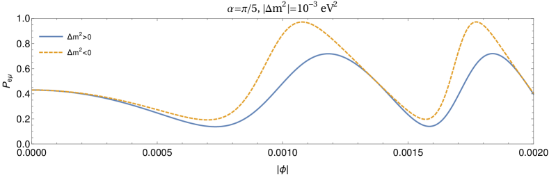
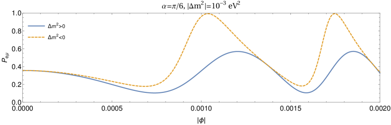
Figure 2: Probability of $\nu_{e}\to\nu_{\mu}$ conversion as function of azimuthal angle $\phi$ for the normal and inverted ordering of neutrino masses in the two flavour case. Here, $R_{s}=3$ km, $r_{D}=10^{8}$ km, $r_{S}=10^{5}r_{D}$ and $E_{0}=10$ MeV. The lightest neutrino is assumed to be massless.

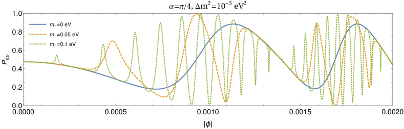
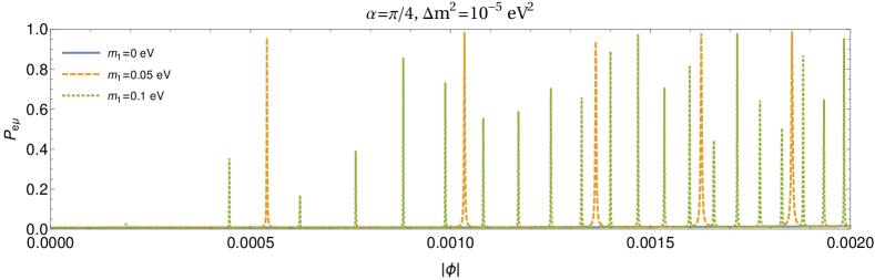
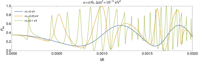
Figure 3: Probability of $\nu_{e}\to\nu_{\mu}$ conversion as function of azimuthal angle $\phi$ for different different values of $m_{1}$ and for $\Delta m^{2}>0$. Here, $R_{s}=3$ km, $r_{D}=10^{8}$ km, $r_{S}/r_{D}=10^{5}$ and $E_{0}=10$ MeV.

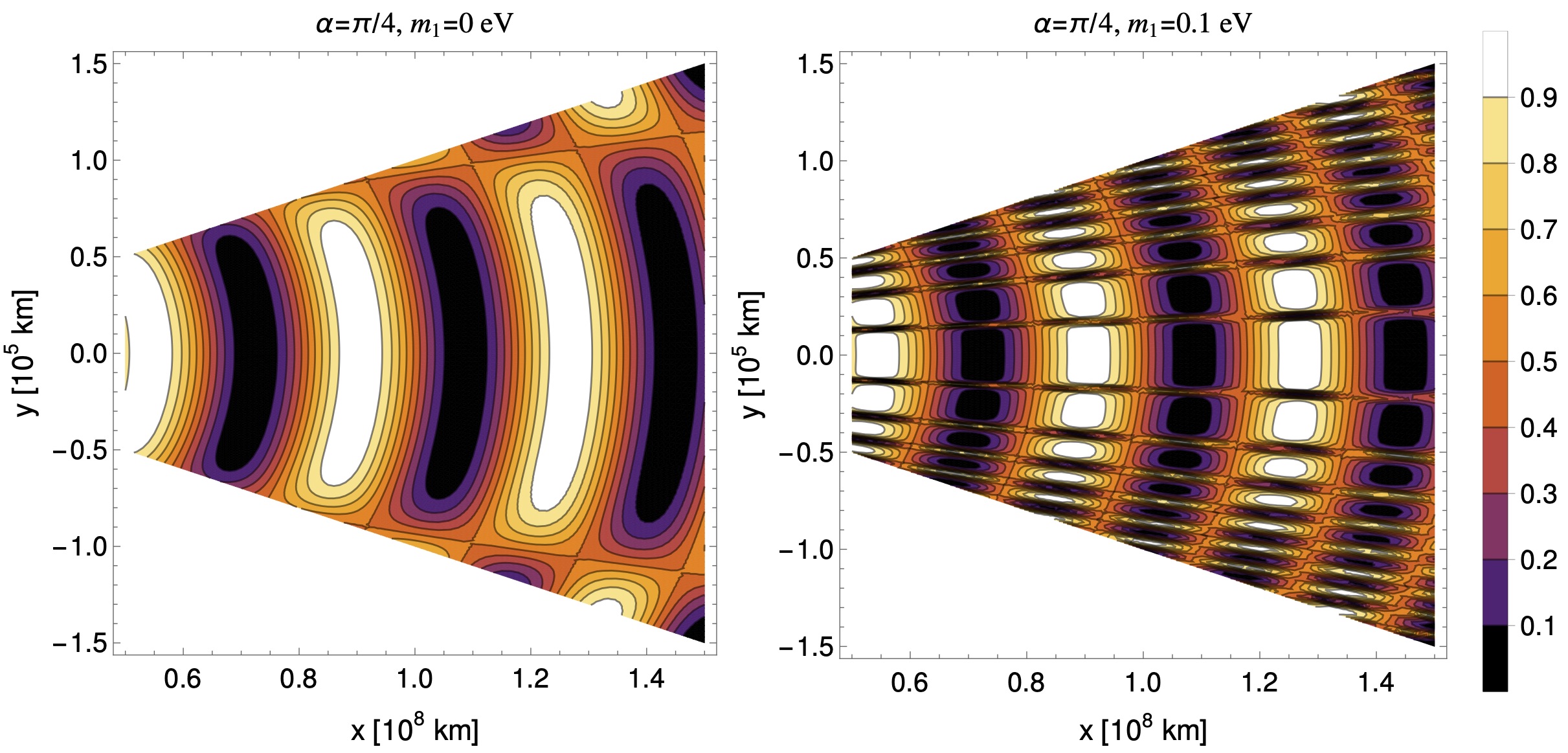
Figure 4: Contours of $\nu_{e}\to\nu_{\mu}$ conversion probability in the presence of gravitational lensing for $R_{s}=3$ km, $r_{D}=10^{8}$ km, $r_{S}=10^{5}\,r_{D}$ and $E_{0}=10$ MeV. Here, $(x_{D},y_{D})$ is location of observer in equatorial plane.

The dependence of conversion probability on the neutrino mass ordering for non-maximal $\alpha$ is shown in Fig. 2. Away from $\phi=0$, the observer is not in the same line of the source and gravitational object which give rise to different probabilities for normal and inverted mass orderings. For $\alpha<\pi/4$, the inverted ordering always corresponds to relatively increased conversion probability than that of the normal ordering. This is due to the fact that $B_{11}<B_{22}$ in Eq. (22) for inverted ordering enhances ${\cal P}^{\rm lens}_{e\mu}$ for $\alpha<\pi/4$. This trend gets reversed if $\alpha>\pi/4$ as Eq. (22) is invariant under simultaneous transformations, $m_{1,2}\to m_{2,1}$ and $\alpha\to\pi/2-\alpha$. It is clear that if the mixing angle is different from $\pi/4$, one can infer the neutrino mass ordering from the lensing effects even in two flavour case in contrast to the standard neutrino oscillations in vacuum without lensing. On the paths independent of $\sum m^{2}$, e.g. along $\phi=0$, the probabilities depend upon (and thus reveal) the standard neutrino oscillation parameters (path length, $\Delta m^{2}$, energy). However, as discussed above, there are other paths which carry imprint of absolute masses as well as the signature of $\Delta m^{2}$ depending upon the mixing angle. Thus, overall observation of probabilities along various directions in the plane of lensing is quite resourceful for neutrino physics.

The lensing of neutrinos is not only sensitive to the neutrino mass ordering but it can also shed light on the absolute mass scale of the neutrinos. As it is shown in Fig. 3, for fixed $\alpha$ and $\Delta m^{2}$, the probability itself oscillates as one goes further from $\phi=0$. The frequency of these oscillations depend on the absolute mass scale of the neutrino. We find that the probability oscillates slowly for hierarchical neutrinos, i.e. $m_{1}\ll\sqrt{\Delta m^{2}}$, when compared to the case when neutrinos are almost degenerate, i.e. $m_{1}\>\raisebox{-4.73611pt}{$\stackrel{{\scriptstyle\textstyle>}}{{\sim}}$}\>\sqrt{\Delta m^{2}}$. This qualitative feature is more or less independent from the specific values of $\alpha$ and $\Delta m^{2}$ as it can be seen from Fig. 3. In the two flavour case, it is therefore possible to infer the absolute neutrino masses by measuring the neutrino transition or survival probabilities with respect to the angle $\phi$.

We also show the probability distribution as function of $(x_{D},y_{D})$ in equatorial plane in Fig. 4. The values of $y_{D}$ and $x_{D}$ are chosen such that they satisfy the weak lensing limit. As it is expected, the maxima and minima of the probability along $y_{D}=0$ line do not depend on the absolute value of neutrino masses. The lensing effect however give rises to different frequencies of maxima and minima of oscillation probabilities for different values of absolute neutrino mass as one deviates from $y_{D}=0$.

V Three flavour case: Numerical Results

In this section, we report results obtained for neutrino lensing in the three flavour case. The geometrical setup and the values of parameters used are same as in the two flavour case discussed in the previous section. For neutrino masses and mixing parameters, we use the values from the latest fit (NuFIT 4.1 (2019)) of neutrino oscillation data Esteban et al. (2019). These are $\Delta m_{21}^{2}=7.39\times 10^{-5}~{}{\rm eV}^{2}$, $\theta_{12}=33.82^{\circ}$, $\Delta m_{31}^{2}=2.523\times 10^{-3}~{}{\rm eV}^{2}$ ($\Delta m_{32}^{2}=-2.510\times 10^{-3}~{}{\rm eV}^{2}$), $\theta_{23}=48.3^{\circ}$ ($\theta_{23}=48.8^{\circ}$), $\theta_{13}=8.61^{\circ}$ ($\theta_{13}=8.64^{\circ}$), $\delta_{\rm CP}=222^{\circ}$ ($\delta_{\rm CP}=282^{\circ}$) for normal (inverted) ordering. The mixing matrix $U$ in three flavour case is evaluated using these mixing parameters and used to obtain the oscillation probabilities using Eq. (20) in equatorial plane. We compute conversion probabilities for $\nu_{e}\to\nu_{\mu}$, $\nu_{\mu}\to\nu_{\tau}$ and $\nu_{e}\to\nu_{\tau}$ for normal and inverted ordering and for two values of the lightest neutrino masses in each case. The results are shown in Fig. 5.

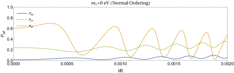
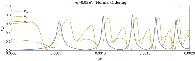
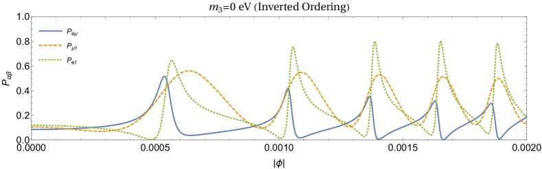
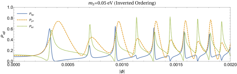
Figure 5: Probability of $\nu_{\alpha}\to\nu_{\beta}$ conversion, for different $\alpha$ and $\beta$, as function of azimuthal angle $\phi$ in three flavour case. We take $R_{s}=3$ km, $r_{D}=10^{8}$ km, $r_{S}=10^{5}r_{D}$ and $E_{0}=10$ MeV. The values of neutrino mass squared differences, mixing angle and the Dirac CP phase are taken from the latest (NuFIT 4.1 (2019)) global fit Esteban et al. (2019).

It can be noticed that the frequency of the oscillations of probabilities increases as the lightest neutrino mass is increased from 0 to 0.05 eV in both the cases of normal and inverted ordering. This is qualitatively in agreement with the two flavour case. Unlike in the two flavour case, one obtains different values of transition probabilities for normal and inverted ordering even for $\phi=0$. Different ${\cal P}_{\alpha\beta}$ then oscillate differently for nonzero $\phi$ as it can be seen from Fig. 5. The mass of the lightest neutrino in both the cases can be inferred by measuring the frequency of the oscillation of transition probabilities.

Throughout this paper, the neutrino wave functions are assumed plane waves. A more realistic treatment of the neutrino oscillations would involve wave packet approach in which neutrinos are produced and detected as wave packets of finite sizes in the position space Giunti and Kim (1998); Akhmedov and Smirnov (2009, 2011). This can give rise to decoherence of neutrinos when propagation over long distances is involved which ultimately leads to wash-out of the flavour oscillations. In flat spacetime and for the gaussian wave packets, the length over which neutrinos maintain coherence is typically given by

$$L_{\rm coh}\simeq 4\sqrt{2}\sigma_{x}E_{0}^{2}/|\Delta m_{ij}^{2}|\,,$$ (31)

where, $\sigma_{x}^{2}\equiv\sigma_{xS}^{2}+\sigma_{xD}^{2}$. Here, $\sigma_{xS}$ represents the position space width of the neutrino wave packet produced at the source while $\sigma_{xD}$ denotes the same for the neutrino at the detector Giunti and Kim (1998). The same expression of coherence length continues to hold in the case of Schwarzschild geometry but with the flat spacetime distance $L_{\rm coh}$ replaced by coordinate distance Chatelain and Volpe (2019).

Following these results we find that the coherence condition, in the weak gravity limit, is given by

$$(r_{S}+r_{D})\left(1-\frac{b^{2}}{2r_{S}r_{D}}+\frac{2GM}{r_{S}+r_{D}}\right)\,<\,\frac{4\sqrt{2}\sigma_{x}E_{0}^{2}}{|\Delta m_{ij}^{2}|}\,.$$ (32)

Further, the terms of ${\cal O}\left(\frac{b^{2}}{r_{S}r_{D}}\right)$ and ${\cal O}\left(\frac{GM}{r_{S}+r_{D}}\right)$ in the above are negligible for the weak lensing cases. Therefore, the treatment of decoherence of neutrinos in the presence of weak lensing is similar to that in flat spacetime. For the typical values of parameters considered in the paper, i.e. $r_{S}+r_{D}\simeq 10^{13}$ km, $E_{0}\simeq 10$ MeV and $|\Delta m_{ij}^{2}|\simeq 10^{-3}$ eV², one obtains $\sigma_{x}\simeq 1.8$ cm. Using $\sigma_{x}\sigma_{p}\sim\hbar$ where $\sigma_{p}$ is the width of neutrino wave packet in the momentum space, the above value of $\sigma_{x}$ would imply neutrino wave packets with $\sigma_{p}/p\lesssim{\cal O}(10^{-11})$ at the source and detector in order to satisfy the coherence condition, Eq. (32). Therefore, this would require very precise information about the energies or meomenta of particles involved in the production and detection processes of neutrinos.

VI Conclusions

Neutrino flavour oscillation in flat spacetime is known to depend on the difference between the squared masses and not on the individual masses of neutrinos. We show that weak gravitational lensing of neutrinos modifies this standard picture drastically. The oscillation probabilities evaluated in the presence of lensing introduces novel effects which depend on the absolute neutrino mass scale in general. We demonstrate this explicitly considering a Schwarzschild mass as a gravitational source for lensing, while the source and detector for neutrinos are kept at finite distances from it. In the presence of Schwarzschild mass, the neutrinos produced at source take more than one classical path to reach to the detector through weak lensing, as justified by the Eikonal approximation. Neutrinos travelling along different trajectories develop different phases which give rise to interference at the location of the detector. We show that the phase difference not only depends on difference of squared neutrino masses but also depends on the individual neutrino masses in general. The dependency on the individual neutrino masses survives for wide class of trajectories of the detector including the geodesic ones. Therefore, the detectors situated on the Keplerian orbits around the Schwarzschild mass will be capable of revealing the absolute mass of neutrinos through measurements of flavour transition probabilities.

We derive the general expression of interference of oscillation probability, valid in the weak lensing limit, for $N$ neutrino flavours and arbitrary number of paths. We study the interference pattern in detail considering the equatorial plane for simplicity in which neutrinos are confined to travel along two trajectories. For $N=2$, we show that the lensing probability is sensitive to the sign of $\Delta m^{2}$ unlike in the case of standard neutrino oscillation in vacuum. Further, it also depends on the individual masses when source, gravitating object and detector are not collinear. flavour transition or survival probabilities oscillate as a result of interference when the detector moves away from the collinear axis. The frequency of these oscillations of probabilities depend on the absolute mass scale of neutrinos. We find that the hierarchical neutrinos, i.e. $m_{1}\ll m_{2}$, give rise to slower oscillations of probability in comparison to the case when they are almost degenerate, i.e. $m_{1}\simeq m_{2}$. We study these effects quantitatively considering the sun-earth like system in which the sun plays role of Schwarzschild mass for neutrinos coming from a distant source. We also give numerical results for $N=3$ which also captures the qualitative effects of lensing obtained in the case of two flavours. All these novel effects are indeed gravitationally induced as they vanish in the flat space ($R_{s}\to 0$) limit. We, therefore conclude that the study of effects of gravitation in the standard analysis of neutrino oscillations can be very resourceful and informative.

Although our results reveal some very non-trivial aspects of neutrino oscillation in the presence of gravitational lensing, a more careful realistic treatment would be required before they can be used for real experimental tests. Firstly, we have adopted the standard practice of using quantum mechanical treatment for the neutrinos in the present study. However, justifiably a quantum field theoretic treatment Grimus et al. (1999); Kobach et al. (2018); Grimus (2019) would be more appropriate. Such a treatment would take into account the mode propagation and will take us out of the limitation of Eikonal validity of using classical trajectories. It may also provide insight to novel phenomenon of gravitational particle creation and the resulting mixing of flavour as well as energy modes due to this particle creation Blasone et al. (2017, 2018a); Cozzella et al. (2018); Blasone et al. (2018b, 2020), etc.. A more realistic treatment of neutrino oscillation with/without lensing should consider the wave packet approach. This, however, relies on the details of the exact mechanisms of neutrino production and detection. As mentioned earlier, such a treatment naturally accounts for the decoherence effects and washing out of oscillation. A detailed study addressing all the above aspects is beyond the scope of this paper and it should be taken up elsewhere.

Appendix A Eikonal Approximation

The classical Hamilton Jacobi function $S(x,p)=\int p_{\mu}dx^{\mu}$ satisfies $\partial S/\partial x^{\mu}=p_{\mu}$. Therefore, classically we have,

$$p_{\mu}p^{\mu}=m^{2}\Rightarrow g^{\mu\nu}\frac{\partial S}{\partial x^{\mu}}\frac{\partial S}{\partial x^{\nu}}-m^{2}=0.$$ (33)

On the other hand the squared Dirac equation satisfies,

$$\left[\partial_{\mu}\partial^{\mu}+m^{2}\right]\psi=0.$$ (34)

If the wavefunction is taken as $\psi=e^{iS/\hbar}$ then

$$\left[g^{\mu\nu}\frac{\partial S}{\partial x^{\mu}}\frac{\partial S}{\partial x^{\nu}}-i\hbar g^{\mu\nu}\partial_{\mu}\partial_{\nu}S-m^{2}\right]\psi=0.$$ (35)

Therefore, as long as

$$\frac{\hbar g^{\mu\nu}\partial_{\mu}\partial_{\nu}S}{g^{\mu\nu}\partial_{\mu}S\partial_{\nu}S}\ll 1,$$

the classical $S$ is a good approximation for the phase of the neutrino. For the massless case $S$ is identically zero and therefore one needs to evaluate the ratio in the limit of small mass $m$. Since for a massive particle

$$S=\Phi(r)=\frac{m^{2}}{2E}\left[r_{S}+r-\frac{b^{2}(r_{S}+r)}{2r_{S}r}+2GM\right],$$ (36)

a naive estimate suggests that the Eikonal approximation will be valid as long as at all the points ($r$) along the path, the condition

$$\left(1-\frac{2GM}{r}\right)\frac{\hbar}{2E}\frac{b^{2}}{r^{3}}\ll 1,$$ (37)

is satisfied. This becomes increasingly valid in weak lensing limit.

Appendix B Observable sensitive to the individual masses: Angle of flavour flipping

An interesting aspect of the transition probability is that in two flavour case Eq. (22), there exists a point where the transition probability from species $\alpha$ to $\beta$ becomes equal to its survival probability $\alpha\rightarrow\alpha$. In other words, one of these two processes remain dominant over some portion of trajectories (indicated by angle $\phi$ in the geodesic trajectory of the earth around the sun in sun-earth system) and then become sub dominant for some other portion. In principle this flipping over occurs multiple times in a trajectory. Therefore, this angle of flipping over (an observable) also carries an imprint of $\sum m^{2}$ which we can utilize and find out the absolute masses. Flipping occurs at point when probability transition and survival probability become equal. For two flavour case, the survival probability is obtained as,

$$P_{\alpha\rightarrow\alpha}=4N^{2}\Bigg{(}\cos^{4}\alpha\cos^{2}\left(m_{1}^{2}\frac{Z\Delta b^{2}}{8E_{0}r_{S}r_{D}}\right)+\sin^{4}\alpha\cos^{2}\left(m_{2}^{2}\frac{Z\Delta b^{2}}{8E_{0}r_{S}r_{D}}\right)$$

$$+2\sin^{2}\alpha\cos^{2}\alpha\cos\left(m_{1}^{2}\frac{Z\Delta b^{2}}{8E_{0}r_{S}r_{D}}\right)\cos\left(m_{2}^{2}\frac{Z\Delta b^{2}}{8E_{0}r_{S}r_{D}}\right)\cos\zeta\Bigg{)},$$ (38)

and the transition probability expression (22) can be cast as

$$P_{\alpha\rightarrow\beta}=4N^{2}\sin^{2}\alpha\cos^{2}\alpha\Bigg{(}\cos^{2}\left(m_{1}^{2}\frac{Z\Delta b^{2}}{8E_{0}r_{S}r_{D}}\right)+\cos^{2}\left(m_{2}^{2}\frac{Z\Delta b^{2}}{8E_{0}r_{S}r_{D}}\right)$$

$$-2\cos\left(m_{1}^{2}\frac{Z\Delta b^{2}}{8E_{0}r_{S}r_{D}}\right)\cos\left(m_{2}^{2}\frac{Z\Delta b^{2}}{8E_{0}r_{S}r_{D}}\right)\cos\zeta\Bigg{)},$$ (39)

where $\zeta\equiv\frac{\Delta m^{2}}{2E_{0}}\left(Z+R_{s}-\frac{Z\sum b^{2}}{4r_{S}r_{D}}\right)$ and $Z=r_{S}+r_{D}$. Therefore, the condition for flipping over is obtained as

$$\cos 2\alpha\cos^{2}\alpha\frac{\cos\left(m_{1}^{2}\frac{Z\Delta b^{2}}{8E_{0}r_{S}r_{D}}\right)}{\cos\left(m_{2}^{2}\frac{Z\Delta b^{2}}{8E_{0}r_{S}r_{D}}\right)}-\cos 2\alpha\sin^{2}\alpha\frac{\cos\left(m_{2}^{2}\frac{Z\Delta b^{2}}{8E_{0}r_{S}r_{D}}\right)}{\cos\left(m_{1}^{2}\frac{Z\Delta b^{2}}{8E_{0}r_{S}r_{D}}\right)}+\sin^{2}2\alpha\cos\zeta=0.$$ (40)

For $\alpha\neq\pi/4$, the above equation can be inverted as

$$\sum m^{2}=\frac{16n\pi E_{0}r_{S}r_{D}}{Z\Delta b^{2}}+\frac{16E_{0}r_{S}r_{D}}{Z\Delta b^{2}}\cot^{-1}\left(\tan\left(\frac{\Delta m^{2}Z\Delta b^{2}}{16E_{0}r_{S}r_{D}}\right)G(r_{S},r_{D},\phi,\alpha,\Delta m^{2},R_{s})\right),$$

(41)

where

$$G(r_{S},r_{D},\phi,\alpha,\Delta m^{2},R_{s}) \equiv \frac{2\cos 2\alpha\cos^{2}\alpha-\sin^{2}2\alpha\cos\zeta\pm\sqrt{\sin^{4}2\alpha\cos^{2}\zeta+\sin^{2}2\alpha\cos^{2}2\alpha}}{2\cos 2\alpha\cos^{2}\alpha+\sin^{2}2\alpha\cos\zeta\mp\sqrt{\sin^{4}2\alpha\cos^{2}\zeta+\sin^{2}2\alpha\cos^{2}2\alpha}}.$$

Similarly, for $\alpha=\pi/4$ we get

$$\left(\cos\left(\frac{\sum m^{2}Z\Delta b^{2}}{8E_{0}r_{S}r_{D}}\right)+\cos\left(\frac{\Delta m^{2}Z\Delta b^{2}}{8E_{0}r_{S}r_{D}}\right)\right)\cos\zeta=0.$$ (43)

Flipping point is given by above equation when either first term or second term is zero, or both. If we find point where first term if zero then, we have

$$\sum m^{2}=\frac{(2n+1)8E_{0}r_{S}r_{D}}{Z\Delta b^{2}}\pi\pm\Delta m^{2},$$ (44)

since the cosine term is symmetric under $\Delta m^{2}\to-\Delta m^{2}$. Therefore,

$$m_{1,2}^{2}=\left(\frac{(2n+1)8E_{0}r_{S}r_{D}}{Z\Delta b^{2}}\right)\frac{\pi}{2}.$$ (45)

For $\cos\zeta=0,$ we cannot determine value of $\sum m^{2}$ because $\zeta$ only involves $\Delta m^{2},E_{0}$ and other terms which involves geometrical points and geometry. As can be seen, in Eq. (41) and Eq. (44) all the direct observable quantities are on the right hand sides, while $n\in\mathcal{Z}$. Thus, the observation of flip angle $\phi$ for known $r_{S},r_{D},\alpha,E_{0},R_{s}\text{ and }\Delta m^{2}$ will reveal $\sum m^{2}$ (upto an ambiguity due to undetermined value of $n$, which have to settled through some independent observations such as Roy Choudhury and Choubey (2018)) which along with information of $\Delta m^{2}$ can give the absolute masses of the neutrinos.

References

- Capozzi et al. (2014) F. Capozzi, G. L. Fogli, E. Lisi, A. Marrone, D. Montanino, and A. Palazzo, “Status of three-neutrino oscillation parameters, circa 2013,” Phys. Rev. D89, 093018 (2014), arXiv:1312.2878 [hep-ph] .
- de Salas et al. (2018) P. F. de Salas, D. V. Forero, C. A. Ternes, M. Tortola, and J. W. F. Valle, “Status of neutrino oscillations 2018: 3 hint for normal mass ordering and improved CP sensitivity,” Phys. Lett. B782, 633–640 (2018), arXiv:1708.01186 [hep-ph] .
- Esteban et al. (2019) Ivan Esteban, M. C. Gonzalez-Garcia, Alvaro Hernandez-Cabezudo, Michele Maltoni, and Thomas Schwetz, “Global analysis of three-flavour neutrino oscillations: synergies and tensions in the determination of , , and the mass ordering,” JHEP 01, 106 (2019), arXiv:1811.05487 [hep-ph] .
- Tanabashi et al. (2018) M. Tanabashi et al. (Particle Data Group), “Review of particle physics,” Phys. Rev. D 98, 030001 (2018).
- Aker et al. (2019) M. Aker et al. (KATRIN), “An improved upper limit on the neutrino mass from a direct kinematic method by KATRIN,” Phys. Rev. Lett. 123, 221802 (2019), arXiv:1909.06048 [hep-ex] .
- Dolinski et al. (2019) Michelle J. Dolinski, Alan W. P. Poon, and Werner Rodejohann, “Neutrinoless Double-Beta Decay: Status and Prospects,” Ann. Rev. Nucl. Part. Sci. 69, 219–251 (2019), arXiv:1902.04097 [nucl-ex] .
- Lesgourgues and Pastor (2014) Julien Lesgourgues and Sergio Pastor, “Neutrino cosmology and Planck,” New J. Phys. 16, 065002 (2014), arXiv:1404.1740 [hep-ph] .
- Vagnozzi et al. (2017) Sunny Vagnozzi, Elena Giusarma, Olga Mena, Katherine Freese, Martina Gerbino, Shirley Ho, and Massimiliano Lattanzi, “Unveiling secrets with cosmological data: neutrino masses and mass hierarchy,” Phys. Rev. D96, 123503 (2017), arXiv:1701.08172 [astro-ph.CO] .
- Roy Choudhury and Choubey (2018) Shouvik Roy Choudhury and Sandhya Choubey, “Updated Bounds on Sum of Neutrino Masses in Various Cosmological Scenarios,” JCAP 1809, 017 (2018), arXiv:1806.10832 [astro-ph.CO] .
- Ahluwalia and Burgard (1996a) Dharam Vir Ahluwalia and C. Burgard, “Gravitationally induced quantum mechanical phases and neutrino oscillations in astrophysical environments,” Gen. Rel. Grav. 28, 1161–1170 (1996a), arXiv:gr-qc/9603008 [gr-qc] .
- Ahluwalia and Burgard (1996b) Dharam Vir Ahluwalia and C. Burgard, “About the interpretation of gravitationally induced neutrino oscillation phases,” (1996b), arXiv:gr-qc/9606031 [gr-qc] .
- Grossman and Lipkin (1997) Yuval Grossman and Harry J. Lipkin, “Flavor oscillations from a spatially localized source: A Simple general treatment,” Phys. Rev. D55, 2760–2767 (1997), arXiv:hep-ph/9607201 [hep-ph] .
- Bhattacharya et al. (1996) Tanmoy Bhattacharya, Salman Habib, and Emil Mottola, “Comment on ‘Gravitationally induced neutrino oscillation phases’,” (1996), arXiv:gr-qc/9605074 [gr-qc] .
- Luongo and Stagno (2011) Orlando Luongo and Gabriele V. Stagno, “Neutrino oscillation at the lifshitz point,” Mod. Phys. Lett. A26, 1257–1266 (2011).
- Geralico and Luongo (2012) A. Geralico and O. Luongo, “Neutrino oscillations in the field of a rotating deformed mass,” Phys. Lett. A376, 1239–1243 (2012), arXiv:1202.5408 [gr-qc] .
- Koutsoumbas and Metaxas (2019) George Koutsoumbas and Dimitrios Metaxas, “Neutrino oscillations in gravitational and cosmological backgrounds,” (2019), arXiv:1909.02735 [hep-ph] .
- Cardall and Fuller (1997) Christian Y. Cardall and George M. Fuller, “Neutrino oscillations in curved space-time: An Heuristic treatment,” Phys. Rev. D55, 7960–7966 (1997), arXiv:hep-ph/9610494 [hep-ph] .
- Fornengo et al. (1997) N. Fornengo, C. Giunti, C. W. Kim, and J. Song, “Gravitational effects on the neutrino oscillation,” Phys. Rev. D56, 1895–1902 (1997), arXiv:hep-ph/9611231 [hep-ph] .
- Sorge and Zilio (2007) Francesco Sorge and Silvio Zilio, “Neutrino spin flip around a Schwarzschild black hole,” Class. Quant. Grav. 24, 2653–2664 (2007).
- Lambiase et al. (2005) G. Lambiase, G. Papini, Raffaele Punzi, and G. Scarpetta, “Neutrino optics and oscillations in gravitational fields,” Phys. Rev. D71, 073011 (2005), arXiv:gr-qc/0503027 [gr-qc] .
- Zhang and Li (2016) Yu-Hao Zhang and Xue-Qian Li, “Three-generation neutrino oscillations in curved spacetime,” Nucl. Phys. B911, 563–581 (2016), arXiv:1606.05960 [hep-ph] .
- Lambiase (2001) G. Lambiase, “Neutrino oscillations in non-inertial frames and the violation of the equivalence principle. Neutrino mixing induced by the equivalence principle violation,” Eur. Phys. J. C19, 553–560 (2001).
- Bhattacharya et al. (1999) Tanmoy Bhattacharya, Salman Habib, and Emil Mottola, “Gravitationally induced neutrino oscillation phases in static space-times,” Phys. Rev. D59, 067301 (1999).
- Crocker et al. (2004) Roland M. Crocker, Carlo Giunti, and Daniel J. Mortlock, “Neutrino interferometry in curved space-time,” Phys. Rev. D69, 063008 (2004), arXiv:hep-ph/0308168 [hep-ph] .
- Alexandre and Clough (2018) Jean Alexandre and Katy Clough, “Black hole interference patterns in flavor oscillations,” Phys. Rev. D98, 043004 (2018), arXiv:1805.01874 [hep-ph] .
- Dvornikov (2019) Maxim Dvornikov, “Spin effects in neutrino gravitational scattering,” (2019), arXiv:1911.08317 [hep-ph] .
- Akhmedov and Smirnov (2009) Evgeny Kh. Akhmedov and Alexei Yu. Smirnov, “Paradoxes of neutrino oscillations,” Phys. Atom. Nucl. 72, 1363–1381 (2009), arXiv:0905.1903 [hep-ph] .
- Akhmedov and Smirnov (2011) E. Kh. Akhmedov and A. Yu. Smirnov, “Neutrino oscillations: Entanglement, energy-momentum conservation and QFT,” Found. Phys. 41, 1279–1306 (2011), arXiv:1008.2077 [hep-ph] .
- Lipkin (2000) H. J. Lipkin, “Neutrino oscillations as two-slit experiments in momentum space,” Phys. Lett. B477, 195–200 (2000).
- Chakraborty (2015) Sumanta Chakraborty, “Aspects of Neutrino Oscillation in Alternative Gravity Theories,” JCAP 1510, 019 (2015), arXiv:1506.02647 [gr-qc] .
- Giunti and Kim (1998) C. Giunti and C. W. Kim, “Coherence of neutrino oscillations in the wave packet approach,” Phys. Rev. D58, 017301 (1998), arXiv:hep-ph/9711363 [hep-ph] .
- Chatelain and Volpe (2019) Amélie Chatelain and Maria Cristina Volpe, “Neutrino decoherence in presence of strong gravitational fields,” (2019), 10.1016/j.physletb.2019.135150, arXiv:1906.12152 [hep-ph] .
- Smirnov (2005) A.Yu. Smirnov, “The MSW effect and matter effects in neutrino oscillations,” Phys. Scripta T 121, 57–64 (2005), arXiv:hep-ph/0412391 .
- Grimus et al. (1999) W. Grimus, P. Stockinger, and S. Mohanty, “The Field theoretical approach to coherence in neutrino oscillations,” Phys. Rev. D59, 013011 (1999), arXiv:hep-ph/9807442 [hep-ph] .
- Kobach et al. (2018) Andrew Kobach, Aneesh V. Manohar, and John McGreevy, “Neutrino Oscillation Measurements Computed in Quantum Field Theory,” Phys. Lett. B783, 59–75 (2018), arXiv:1711.07491 [hep-ph] .
- Grimus (2019) Walter Grimus, “Revisiting the quantum field theory of neutrino oscillations in vacuum,” (2019), arXiv:1910.13776 [hep-ph] .
- Blasone et al. (2017) Massimo Blasone, Gaetano Lambiase, and Giuseppe Gaetano Luciano, “Nonthermal signature of the Unruh effect in field mixing,” Phys. Rev. D96, 025023 (2017), arXiv:1703.09552 [hep-th] .
- Blasone et al. (2018a) Massimo Blasone, Gaetano Lambiase, Giuseppe Gaetano Luciano, and Luciano Petruzziello, “Neutrino oscillations in accelerated frames,” EPL 124, 51001 (2018a), arXiv:1812.09697 [hep-ph] .
- Cozzella et al. (2018) Gabriel Cozzella, Stephen A. Fulling, André G. S. Landulfo, George E. A. Matsas, and Daniel A. T. Vanzella, “Unruh effect for mixing neutrinos,” Phys. Rev. D97, 105022 (2018), arXiv:1803.06400 [gr-qc] .
- Blasone et al. (2018b) Massimo Blasone, Gaetano Lambiase, Giuseppe Gaetano Luciano, and Luciano Petruzziello, “Role of neutrino mixing in accelerated proton decay,” Phys. Rev. D97, 105008 (2018b), arXiv:1803.05695 [hep-ph] .
- Blasone et al. (2020) M. Blasone, G. Lambiase, G. G. Luciano, and L. Petruzziello, “Neutrino oscillations in the Unruh radiation,” Phys. Lett. B800, 135083 (2020), arXiv:1903.03382 [hep-th] .