Calibration Method and Uncertainty for the Primordial Inflation Explorer (PIXIE)

Abstract

The Primordial Inflation Explorer (PIXIE) is an Explorer-class mission concept to measure cosmological signals from both linear polarization of the cosmic microwave background and spectral distortions from a perfect blackbody. The targeted measurement sensitivity is 2–4 orders of magnitude below competing astrophysical foregrounds, placing stringent requirements on instrument calibration. An on-board blackbody calibrator presents a polarizing Fourier transform spectrometer with a known signal to enable conversion of the sampled interference fringe patterns from telemetry units to physical units. We describe the instrumentation and operations needed to calibrate PIXIE, derive the expected uncertainty for the intensity, polarization, and frequency scales, and show the effect of calibration uncertainty in the derived cosmological signals. In-flight calibration is expected to be accurate to a few parts in $10^{6}$ at frequencies dominated by the CMB, and a few parts in $10^{4}$ at higher frequencies dominated by the diffuse dust foreground.

1 Introduction

The cosmic microwave background (CMB) provides a unique window to the early universe. Its blackbody spectrum points to a hot, dense phase in the early universe, while spatial maps of small temperature perturbations about the blackbody mean provide detailed information on the geometry, constituents, and evolution of the universe.

New measurements could provide additional insight. Maps of CMB polarization trace a stochastic background of gravitational radiation produced during an inflationary epoch in the early universe, testing physics at energies above $10^{15}$ GeV while providing the first observational evidence for quantum gravity[1, 2, 3]. Small deviations from the monopole blackbody spectrum (spectral distortions) record energy transfers between the evolving matter and radiation fields to detail the thermal history of the universe[4].

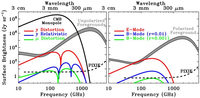
Figure 1: Cosmological signals are faint compared to the combined foreground emission. (left) Unpolarized CMB spectral distortions from the Compton y distortion caused by scattering in groups and clusters, the relativistic correction to the y distortion, and the $\mu$ distortion from dissipation of primordial density perturbations. (right) Polarized signals from density perturbations (E-modes) and inflation (B-modes). The PIXIE noise level is shown for 12 months cumulative integration time in each observing mode.

The cosmological signals for both polarization and spectral distortions are small compared to astrophysical foregrounds (Figure 1). CMB polarization can be decomposed into a parity-even (E-mode) component sourced by primordial density perturbations and a parity-odd (B-mode) component sourced by inflation. For the simplest (single-field) inflation models, the amplitude of the B-mode signal depends on the energy scale of inflation as

$$E=1.06\times 10^{16}\left(\frac{r}{0.01}\right)^{1/4}~{}{\rm GeV}\vspace{-2mm}$$ (1.1)

where $r$ is the power ratio of gravitational waves to density fluctuations [1]. Current measurements set upper limits $r<0.07$ [5], while next-generation experiments look for sensitivity $r\ll 10^{-3}$. Spectral distortions result from energy injection in the early universe that drives the matter and radiation fields out of thermal equilibrium. The simplest distortions result from Compton scattering of CMB photons from relativistic electrons and are characterized by the Compton $y$ parameter for the optically-thin case and the Bose-Einstein chemical potential $\mu$ for the optically thick case[6, 7]. Current upper limits $|y|<15\times 10^{-6}$ and $|\mu|<9\times 10^{-5}$ correspond to fractional deviations $\Delta I/I$ less than 50 parts per million in the CMB blackbody spectrum[8]. Measurements with background-limited detectors could improve these limits by several orders of magnitude, opening a broad discovery space[4, 9].

Distinguishing cosmological signals from the competing foregrounds based on their different frequency dependence requires measurements over a broad frequency range. At levels of a few nK in thermodynamic temperature (1 Jy sr^-1 or 10^-26 W m^-2 Hz^-1 sr^-1), the targeted measurement sensitivity for next-generation measurements is 2–4 orders of magnitude or more below the foreground amplitude, placing stringent requirements on instrument dynamic range and calibration.

Calibration presents an instrument with a known signal, enabling the conversion of sampled data from digitized telemetry units to physical units. In-flight calibration of previous space-based CMB missions has relied on observations of on-board blackbody sources [10], astrophysical sources such as the Moon or planets [11, 12, 13], or the CMB dipole induced by the motion of the spacecraft or Solar System with respect to the CMB rest frame [11, 14, 15, 13]. Three aspects of the calibration are particularly important: The absolute calibration which converts data from digitized telemetry units to physical units, the relative calibration or uncertainty in the calibration between measurements in different frequency channels, and the frequency calibration or extent to which the frequency scale and passbands of individual frequency channels are known.

The Primordial Inflation Explorer (PIXIE) is an Explorer-class mission concept to characterize both CMB polarization and spectral distortions [16]. PIXIE represents an updated, fully symmetric version of the seminal Far Infrared Absolute Spectrophotometer (FIRAS) flown on the Cosmic Background Explorer[17]. Room-temperature versions[18] validate the the optical design, which we supplement using simulations and data from balloon-borne cryogenic instruments[19, 22]. This paper describes the instrumentation and techniques to calibrate the PIXIE data, derives the expected uncertainty in the calibration, and shows the effect of calibration uncertainty on the extracted cosmological signals.

2 The PIXIE Instrument

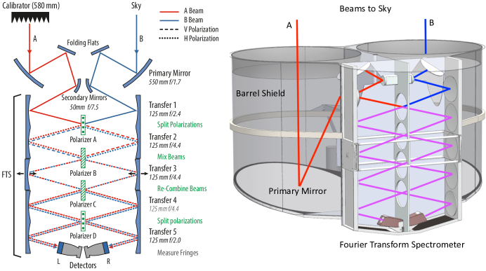
Figure 2: Schematic rendering of the PIXIE instrument, showing the proposed optical path (left) and the beam-forming optics (right). The signal path after the first polarizer consists of linear combinations of orthogonal polarization states (dashed vs dotted lines) from the two input ports (red vs blue lines). Linear combinations on the left side of the instrument are orthogonal to those on the right side.

Figure 2 shows the PIXIE instrument concept. It consists of a polarizing Fourier transform spectrometer (FTS) with two input ports illuminated by co-pointed beams on the sky. A set of polarizing wire grids splits each beam into orthogonal liner polarizations then mixes the beams. A pair of movable mirrors introduces an optical phase delay before a second set of polarizing grids recombines the beams and routes them to a pair of polarization-sensitive detectors at each of the two output ports. As the phase-delay mirrors sweep back and forth, each of the 4 detectors samples the resulting interference fringe pattern as a function of the optical phase delay. Let $\vec{E}=E_{x}\hat{x}+E_{y}\hat{y}$ represent the electric field incident from the sky. The power $P$ at the detectors as a function of the phase delay $z$ may be written

$$P_{Lx} = 1/2~{}\smallint\{~{}(E_{Ax}^{2}+E_{By}^{2})+(E_{Ax}^{2}-E_{By}^{2})\cos(z\omega/c)~{}\}d\omega$$

$$P_{Ly} = 1/2~{}\smallint\{~{}(E_{Ay}^{2}+E_{Bx}^{2})+(E_{Ay}^{2}-E_{Bx}^{2})\cos(z\omega/c)~{}\}d\omega$$

$$P_{Rx} = 1/2~{}\smallint\{~{}(E_{Ay}^{2}+E_{Bx}^{2})+(E_{Bx}^{2}-E_{Ay}^{2})\cos(z\omega/c)~{}\}d\omega$$

$$P_{Ry} = 1/2~{}\smallint\{~{}(E_{Ax}^{2}+E_{By}^{2})+(E_{By}^{2}-E_{Ax}^{2})\cos(z\omega/c)~{}\}d\omega~{},$$ (2.1)

where $\hat{x}$ and $\hat{y}$ refer to orthogonal linear polarizations, L and R refer to the detectors in the left and right concentrators, A and B refer to the two input beams, and $\omega$ is the angular frequency of incident radiation. The optical phase delay $z$ is related to the physical mirror position $\Delta L$ as

$$z=4\cos(\theta)\cos(\delta/2)\Delta L~{},$$ (2.2)

where $\theta$ is the angle of incident radiation with respect to the mirror movement, $\delta$ is the dispersion in the beam, and the factor of 4 reflects the symmetric folding of the optical path. The factor of $1/2$ rather than $1/4$ for each of the four detectors results from use of 2 input ports rather than a single port. When both input ports are open to the sky, the power at each detector consists of a dc term proportional to the intensity $E_{x}^{2}+E_{y}^{2}$ (Stokes $I$) plus a term modulated by the phase delay $z$, proportional to the linear polarization $E_{x}^{2}-E_{y}^{2}$ (Stokes $Q$) in instrument-fixed coordinates. Rotation of the instrument about the beam axis rotates the instrument coordinate system relative to the sky to allow separation of Stokes $Q$ and $U$ parameters on the sky. A full-aperture calibrator can be deployed to block either of the two input ports, or stowed so that both ports view the sky. With one input port terminated by a blackbody calibrator, the modulated term is then proportional to the difference between the sky signal and the calibrator, providing sensitivity to the sky signal in Stokes $I$, $Q$, and $U$ as well as a known reference signal for calibration. Scattering filters on the folding flat and secondary mirrors limit the optical passband to truncate the integral in Eq. 2.1. The 30 $\mu$m wire spacing in the polarizing grids additionally limits the response to high-frequency signals. Both effects are included in all calculations below.

2.1 PIXIE Calibrator

Figure 3 shows the calibrator design. It will consist of 1369 absorbing cones mounted on an aluminum backplate 580 mm in diameter. Each cone is 25 mm tall and 16 mm wide at the base, with an aluminum core coated by an absorbing layer. The absorber consists of a combination of graphite, stainless steel, and doped silicon particles 5 $\mu$m in diameter suspended in a matrix of epoxy and silicon dioxide powder [20]. The matrix is tuned so that its coefficient of thermal expansion matches the aluminum core. The aluminum core provides thermal conductivity and mechanical support while allowing easy attachment to the aluminum back plate. Some 40 thermometers mounted in selected cones monitor the temperature across the calibrator.

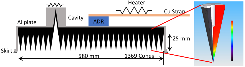
Figure 3: Schematic of PIXIE blackbody calibrator with inset showing front-to-back thermal gradients in a single cone.

Thermal control is maintained using three elements. A copper strap runs from the calibrator to a heat sink maintained at 2.6 K to provide the main cooling path for the calibrator. A resistive heater allows for precise thermal control. A paramagnetic salt pill within a controlled magnetic field acts as a single-stage adiabatic demagnetization refrigerator to provide a reversible source of heat. The magnetic field can be reduced to cool the calibrator below the 2.6 K heat sink, or the field can be increased to heat the calibrator well above the heat sink. Since the heat is stored within the salt pill, raising or lowering the calibrator temperature in this fashion does not inject an additional heat load to the 2.6 K heat sink.

Both the calibrator and the instrument optical path (mirrors, polarizing grids, and surrounding walls) will normally be maintained within a few mK of the CMB monopole temperature, approximating a blackbody cavity. A blackbody is fully characterized by a single parameter, its temperature: in the limit that the instrument and sky are fully isothermal, no fringe pattern can be produced regardless of the position of the mirrors or the emissivity of any portion of the instrument. Deviations from this ideal, whether from the sky or the instrument, will then generate non-zero interferograms (Eq. 2.1), but by approximating an isothermal cavity, PIXIE reduces the required dynamic range and suppresses instrumental effects (systematic errors) from all components following the FTS [21].

A blackbody calibrator at temperatures near 2.725 K provides an excellent match to the CMB, but emits almost no radiation at frequencies above 600 GHz where other astrophysical sources (interstellar dust, the cosmic infrared background, and far-infrared emission lines) become important. Simply raising the calibrator temperature to 20 K would provide photons for the high-frequency calibration, but would also increase the total power on the detectors by a factor of over 1000. Non-linearities in the detector performance would then limit the reliability of the resulting calibration. Instead, PIXIE replaces a single cone with a matching conical cavity which can be heated to higher temperatures. The filling fraction of a single cavity (of order 0.1%) approximates the effective emissivity of the dominant dust foreground, while the choice of a cavity instead of a cone minimizes perturbations from radiative heat transport between the cavity and surrounding cones. Normally the cavity is maintained at the same temperature as the rest of the calibrator. Section 2.2 discusses the high-frequency calibration when the cavity is heated above the CMB temperature.

The PIXIE calibrator design is based on a similar calibrator flown by the ARCADE-2 mission [19], which provides a more compact configuration than the single inverted cone flown by FIRAS [10]. The ARCADE-2 calibrator achieved reflectance between -42 dB at the longest wavelength of 10 cm (3 GHz) and -68 dB at shorter wavelengths, averaging -57 dB across the full band 30–90 GHz [19]. The PIXIE calibrator is expected to achieve reflectance less than $-65$ dB from 15 GHz to 600 GHz, rising to $-50$ dB at higher frequencies. In the long-wavelength limit, the calibrator may be approximated as a smooth impedance transition from free space to the absorber. The ARCADE-2 calibrator used 295 cones each 88 mm tall, requiring the transition to occur over less than one wavelength at the lowest frequency of 3 GHz. For PIXIE at 30 GHz, the transition takes place over 2.5 wavelengths. The measured reflectance of the ARCADE-2 calibrator at a comparable ratio of cone height to wavelength is -68 dB (the noise floor of the measurement). In the short-wavelength (geometric optics) limit, the array of cones can be approximated as a series of surfaces requiring multiple bounces before incident rays can reflect back. Critical parameters are the dielectric loading of the absorber, the number of bounces, and the sharpness of the cone tips and joints between adjacent cones. The ARCADE-2 short-wavelength reflectance of -56 dB is consistent with 6 bounces with $\sim$12% reflection at each bounce. The PIXIE calibrator retains the same number of bounces but tunes the absorber dielectric constant and loading to reduce the surface reflectance at each bounce. Replacing the alumina (Al₂O₃) filler in the ARCADE-2 calibrator with silicon dioxide (SiO₂) for PIXIE reduces the index of refraction in the absorber mixture, lowering the surface reflection by 40%. The limiting factor is expected to be single reflections from the cone tips. The ARCADE-2 cones have a tip radius of 300 $\mu$m. Engineering models of the PIXIE cones demonstrate tip radius below 50 $\mu$m, corresponding to calibrator reflectance -50 dB at frequencies above 600 GHz (wavelength $<500~{}\mu$m). Reflectance is further minimized by staggering the heights of individual cones so that reflections do not add coherently and by tipping the entire calibrator by $\sim$2^∘  so that residual reflections do not propagate directly back through the instrument to the detectors ($\S$3.3).

Temperature gradients within the calibrator are expected to be small. Steady-state thermal gradients require heat transport within the calibrator. The copper strap attaches to the calibrator at a single point: heat transport within the calibrator requires heat to flow from the strap through the absorbing cones and then by radiation to the instrument optics. We estimate the resulting gradients by comparison to the ARCADE-2 calibrator. The balloon-borne ARCADE-2 calibrator operated at altitude 37 km and was surrounded by gaseous helium at pressure $\sim$3 Torr. Temperature control at 2.725 K was maintained by heaters mounted on the back of the calibrator, while the absorbing cones faced metal structures (conical horn antennas and mounting plates) at temperature 1.5 K. Heat flow from the heaters through the absorbing cones and helium gas to the colder metal structures drove back-to-front temperature gradients within the absorbing cones. In-flight data showed heat flow of 1.5 W resulting in 600 mK temperature gradients concentrated near the cone tips [22]. The PIXIE calibrator, in contrast, operates in a vacuum with the absorbing cones facing a nearly isothermal cavity. Radiative transport between the calibrator at 2.725 K and a cavity 5 mK colder produces a heat flow of 0.3 nW, corresponding to maximum back-to-front temperature gradients of 0.1 nK within the absorbing cones (distortion $|y|\sim 10^{-12}$). This is smaller than the thermometer read noise ($\S$3.1) even when averaged over the course of a four-year mission.

In the limit that the calibrator is an open thermal circuit, it cannot support thermal gradients. Energy deposition from cosmic rays traversing the calibrator represent a stochastic internal source of heat to produce thermal gradients across the calibrator. The flux of cosmic ray protons has a steep energy dependence, $dN/dE\approx 0.003~{}(E/10~{}{\rm GeV})^{-2.7}$ cm^-2 sr^-1 s^-1 GeV^-1 at energies above a few GeV, yielding an anticipated rate of order 1 hit per second for a single cone. A single cosmic ray hit will deposit $\sim$50 MeV (8 pJ) into the calibrator, nearly independent of the proton energy. Each cone has heat capacity $5\times 10^{-3}$ J/K. In the absence of thermal averaging a single proton hit would instantaneously raise the temperature of a cone by 2 nK, corresponding to distortion $|y|<10^{-12}$ after accounting for signal dilution from other unaffected cones. In practice, we must account for both the thermal time constant and for multiple cosmic ray hits over the entire calibrator. Averaged over the entire calibrator, we expect $\sim$1000 cosmic ray hits per second, equivalent to an internal heat dissipation of 5 nW. The resulting flow of heat through the calibrator base to the copper strap heat sink creates a radial temperature gradient of order 1 nK across the calibrator, equivalent to a distortion $|y|<10^{-10}$.

Temperature gradients during the high-frequency calibration using the single hot cavity are more difficult to assess. A single calibrator cavity with diameter 16 mm and temperature 20 K will radiate $\sim 0.5~{}\mu$W to the 2.725 K instrument, with negligible radiation from the instrument back to the cavity. If gradients within the calibrator cavity scale comparably to gradients in the absorbing cones, the resulting radiative heat flow would drive back-to-front gradients of order 0.2 mK within the absorbing material of the cavity. Lateral gradients along the cavity walls and from the cavity to nearby cones are likely to be larger than this. A 2 mK lateral gradient within the cavity corresponds to fractional error of order 0.01% in the absolute calibration above 600 GHz. As with ARCADE, lateral gradients in the cones surrounding the cavity can be identified and removed using a principal component analysis of transients excited as the cavity is commanded to different temperatures. A principal component analysis reduced the measured 600 mK front-to-back thermal gradients in the ARCADE-2 calibrator to a 5 mK uncertainty in the calibrator radiometric temperature [22]. A comparable analysis for PIXIE 2 mK gradients would predict uncertainties of order 20 $\mu$K in the high-frequency calibration. Additional analysis of temperature gradients deliberately induced when the calibrator is stowed can further constrain calibrator time constants and thermal profile.

2.2 Calibration Operations

PIXIE will observe from the second Sun-Earth Lagrange point, L2. The phase-delay mirrors complete a full cycle every 3 seconds. The co-pointed beams are maintained perpendicular to the Sun-Earth line. The entire observatory rotates about the beam axis every 48 seconds while simultaneously scanning the beams through a great circle perpendicular to the Sun-Earth line every 384 rotations (approximately 5 hours). The annual motion of the Sun-Earth line precesses the great circle on the ecliptic plane once per year so that the beams map the full sky every 6 months. The fixed relations of 16 mirror cycles per beam rotation and 384 beam rotations per great-circle scan simplify the mapping algorithm but are not required.

Calibration proceeds as follows. At the start of each great-circle scan, the calibrator is set to a new temperature and moved to a new position. Temperature setpoints span the range [2.720, 2.730] K to bracket the CMB monopole at 2.725 K. The calibrator position sequentially deploys through 4 consecutive scans to block the A beam, leave both beams open to the sky, block the B beam, and leave both beams open to the sky again. This pattern gives equal integration time to measurements of CMB polarization (both beams open) and spectral distortions (calibrator over one beam) but can be modified at any time during the mission. We define the start of a scan as either the north or south ecliptic pole, so that changes in temperature and position occur only over regions of the sky observed at every scan. Temperatures for other elements of the instrument can also be changed at the start of each scan ($\S$3.3).

With the calibrator deployed to block one beam, the interferograms depend on the difference between the sky signal and the calibrator. We remove dependence on the sky signal by comparing data from two neighboring scans: one with the calibrator blocking the A beam and a second with the calibrator blocking the B beam. Since input signals change sign when observed in the A beam vs the B beam (Eq. 2.1), the sky signal in each map pixel cancels when summing the scan data for that pixel, leaving only the difference in the calibrator signal. The differential calibrator signal may then be averaged over the scan circle to provide an absolute blackbody reference for signal calibration. Transients following commanded temperature changes and pixels with large sky-signal gradients (e.g. near the Galactic plane) may be excluded from the calibration with only modest loss of effective observing time.

Calibrator excursions of $\pm$5 mK about the mean CMB temperature provide calibration for frequencies below 600 GHz. A small fraction of the observing time (5–10%) is reserved for operations with the entire calibrator at significantly higher or lower temperatures, or with the single inverse cavity heated to higher temperature. These data provide calibration for data above 600 GHz, and will be supplemented by observations of Jupiter, Mars, and Saturn, each of which is observed for 13 consecutive scans twice per year. The total power absorbed by each detector is dominated by the CMB monopole and the calibrator mean temperature; the fringe pattern from 5 mK calibrator excursions changes the detector loading by only 0.7% to minimize effects of detector non-linearities for the low-frequency calibration. When the single cavity is heated to 20 K, the power absorbed by each detector nearly triples. To compensate for this, the temperature of the rest of the calibrator can be lowered so that the total power on the detector remains nearly constant. Comparison of scans at identical detector loading but different cavity temperatures then determines the filling fraction of the single cavity. Selected scans with the entire calibrator maintained at temperatures ranging from 2.5 to 3 K vary the detector loading by 50% to provide channel-by-channel characterization of detector non-linearity so that the calibrated sky spectra are always interpolated and not extrapolated.

3 Calibration Accuracy

The accuracy to which sky signals can be converted from digitized telemetry units to physically meaningful units depends on the signal to noise ratio of the calibration, the accuracy of the temperature scale, and the extent to which non-ideal instrument parameters (reflections, temperature gradients) can be removed. PIXIE will be background-limited, with noise dominated by photon arrival statistics from the CMB and blackbody calibrator. Calibrator temperature excursions of $\pm$5 mK provide a signal-to-noise ratio above $10^{3}$ within individual frequency channels below 600 GHz for a single comparison of two neighboring calibrator scans (Figure 4). Operations with a single hot cavity provide signal to noise ratio up to $10^{6}$ at higher frequencies. Raw sensitivity will not limit the PIXIE calibration. The following sections discuss the impact of various instrumental effects on the PIXIE calibration.

Figure 4: Signal to noise ratio for a single differential calibration scan. The solid line refers to the low-frequency calibration with the entire calibrator maintained within 5 mK of the CMB temperature. The dashed line shows the high-frequency calibration with a single cavity at 20 K. The PIXIE calibration will not be limited by signal to noise ratio.

3.1 Thermometry

The PIXIE calibration rests upon comparison of blackbody loads at different temperatures. The FTS and beam-forming optics, including all walls and baffles, will be maintained at temperatures near the CMB monopole, allowing the temperature readout to be optimized for a relatively narrow range. Thick-film ruthenium oxide resistors with resistance $\sim$50 k$\Omega$ at 2.7 K and 1 pW power dissipation can be read out to precision $\sim 100~{}\mu$K over a one-second integration. A principal component analysis of the ARCADE-2 calibrator showed that 7 well-placed thermometers would be sufficient to characterize both the mean temperature and thermal gradients within the calibrator[22]. The PIXIE calibrator will contain 40 thermometers mounted at different heights in individual cones. The pW power dissipation from each thermometer is small compared to the nW front-to-back heat flow within the calibrator and will not contribute significantly to thermal gradients. Thermometry noise limits knowledge of the calibrator mean temperature to precision 16 $\mu$K for a one-second integration, or 100 nK for a single differential calibration scan. A four-year mission provides over 1600 calibration scans, reducing the thermometry noise to the 2 nK level over the entire mission, corresponding to calibration uncertainty of order $10^{-9}$ within individual frequency channels. The resulting spectral distortion limits $|y|<2\times 10^{-11}$ and $|\mu|<3\times 10^{-10}$ are negligible compared to the instrument noise.

The one-second thermometer sampling is rapid compared to the 20 second thermal time constant of the calibrator. Thermal excursions on shorter time scales (e.g. from energy deposited by cosmic ray hits within the calibrator) are suppressed by the thermal mass and filling fraction of the absorbing cones ($\S$2.1). The expected cosmic ray flux yields stochastic fluctuations 0.2 nW over the course of a 1-second thermometer integration, producing negligible distortions in the calibrator-sky difference spectra.

Careful distinction must be made between thermometer precision vs accuracy. Although the thermometer readout noise integrates down with additional calibration scans (precision), the conversion between thermometer resistance and absolute temperature (accuracy) does not. A well-calibrated cryogenic thermometer will typically reproduce the actual temperature within 100 $\mu$K, leading to comparable uncertainty in the physical temperature of the calibrator. Different calibration scans at different commanded calibrator temperatures bracket the CMB monopole temperature. Over this limited range, the absolute thermometry error may be treated as a constant temperature offset, canceling when comparing calibrator data at different commanded temperatures. By interpolating sky spectra taken at different calibrator temperatures, PIXIE can match the (unknown) monopole temperature to 2 nK precision; however, the inferred monopole temperature will differ from the true temperature by up to 100 $\mu$K. Since the sky signal does not enter the calibration process, this systematic error does not affect the relative calibration.

The absolute thermometry does not depend solely on pre-flight calibration, but can be deduced from in-flight data as well. Calibration data from successive scans with calibrator temperature difference $\Delta T$ generate differential spectra

$$I(\nu,T)=\frac{\partial B_{\nu}}{\partial T}\Delta T$$ (3.1)

where

$$B_{\nu}(T)=\frac{2h\nu^{3}}{c^{2}}\frac{1}{{\rm e}^{x}-1}$$ (3.2)

is the blackbody Planck law, $\nu$ is the observing frequency, $k$ is Boltzmann’s constant, $h$ is the Planck constant, and

$$x=\frac{h\nu}{kT}$$ (3.3)

is the dimensionless frequency, defined using the thermodynamic temperature $T$. We may fit the peak frequency of the observed calibrator spectra and use the Wien displacement law to determine the mean calibrator temperature to 10 $\mu$K accuracy independent of the sky spectra, corresponding to calibration accuracy $2\times 10^{-5}$. Alternatively, we may use the sky-only data to determine the color temperature of the CMB dipole induced by PIXIE’s motion about the sun, which fixes the temperature scale to similar accuracy. Both methods can assess thermometry drifts in time.

The 10 $\mu$K systematic error in the assigned temperature will propagate to CMB spectral distortions, which use the CMB monopole temperature to define the distortion spectral shape. This effect is small. The optically-thin $y$ distortion is defined as

$$I(\nu)=\frac{2h\nu^{3}}{c^{2}}\frac{1}{{\rm e}^{x}-1}\left(1+y\frac{x{\rm e}^{x}}{{\rm e}^{x}-1}\left[\frac{x}{{\rm tanh}(x/2)}-4\right]\right)~{},$$ (3.4)

while the optically thick $\mu$ distortion is

$$I(\nu)=\frac{2h\nu^{3}}{c^{2}}\frac{1}{{\rm e}^{x+\mu}-1}$$ (3.5)

A 10 $\mu$K error in the assigned value for $T_{0}$ creates a negligible fractional error $\Delta I/I<2\times 10^{-5}$ in the recovered $y$ or $\mu$ distortions.

3.2 Temperature Gradients

Temperature gradients within the calibrator produce a superposition of emission from elements at different physical temperatures. The predicted 1 nK radial gradient or 0.1 nK front-to-back gradient produce negligible errors in the absolute calibration: even if the entire calibrator were 1 nK warmer or colder than commanded, the fractional error in the absolute calibration is below $10^{-8}$. However, if not accounted for, the resulting distortion $y\sim 10^{-10}$ from the calibrator itself would induce a false detection of opposite sign in the calibrator–sky comparison. Radial gradients can be identified and subtracted using a principal component analysis during commanded calibrator temperature changes[22]. The sign of the front-to-back temperature gradient depends on the sign of the calibrator–cavity temperature difference, with the cone tips colder than the base when the calibrator is warmer than the cavity and warmer than the base when the calibrator is colder than the cavity. Since the calibrator spends equal amounts of time warmer as colder over the course of the full mission, thermal gradients cancel in the determination of the mean spectral distortion signal and only contribute to the scan-to-scan variance. The predicted effect is negligible compared to the thermometer readout noise.

Gradients in the single hot cavity affect the high-frequency calibration by altering the power incident on the detector. Since these data are used only as a reference for sky signals above the CMB Wien cutoff, they do not directly source a false $y$ distortion. A 2 mK cavity gradient creates a fractional error $7\times 10^{-5}$ in the calibration at frequencies above 600 GHz.

3.3 Reflections

Internal reflections within the calibrator–instrument system create calibration errors by replacing emission from the calibrator with emission from elsewhere within the instrument. Rays that reflect from the calibrator and terminate elsewhere within the instrument create an error signal proportional to the calibrator power reflection coefficient and the temperature difference between the calibrator and the instrument surface where the ray terminates. Most of the instrument is maintained within 5 mK of the calibrator temperature to minimize this effect. A -65 dB calibrator reflection results in a 1.5 nK error signal, corresponding to a fractional error $3\times 10^{-9}$ in the absolute calibration.

As with temperature gradients within the calibrator, reflections to components at different physical temperatures lead to a small $y$ distortion in the calibration signal. Each of the $\sim$20 surfaces in the cryogenic portion of the instrument is individually temperature controlled. The commanded temperatures are periodically varied to allow identification and subtraction of the residual reflected signals, which also maps beam spillover within the instrument [21]. The calibration procedure includes $\sim$20 additional free parameters for the coupling to each internal surface. This number is small compared to the 40 million mirror strokes during the course of the mission, allowing the residual $y$ distortion to be removed to the mission noise limit $|y|<10^{-11}$.

The detector assembly is maintained at 0.1 K and is the only component significantly colder than the calibrator. Approximately 0.3% of the signal reflected by the calibrator (-90 dB of the full signal) propagates back through the FTS to reach the detector. The corresponding 3 nK error signal may be removed to first order using pre-flight measurements of the calibrator reflection, leaving residuals $|y|<10^{-11}$ in the distortion spectra.

The reflection error signal is larger for the high-frequency calibration using the single hot calibrator cavity. Since the 2.725 K instrument has negligible emission above 600 GHz, the fractional error in the high-frequency calibration primarily depends on the power reflection coefficient of the single hot cavity. A -40 dB reflection from the cavity produces fractional errors of $2\times 10^{-5}$ in the high-frequency calibration.

3.4 Leakage

Leakage of external signals into the calibrator/instrument cavity presents an additional perturbation. The CMB monopole dominates the sky at frequencies below 600 GHz. Since the calibrator is maintained within a few mK of the CMB, sky leakage presents a negligible problem. The calibrator and instrument optics are surrounded by a nested set of reflective shields, preventing direct view from the instrument aperture to the Sun or warm portions of the spacecraft. Potential leakage is dominated by the view to the innermost shield, which operates at temperatures near 16 K and subtends 3% of the $2\pi$ sr above the aperture. To minimize leakage, the calibrator extends 2 mm beyond the edge of the aperture with a flexible skirt of aluminized mylar to provide an electromagnetic seal between the calibrator and the aperture. The barrel has a flared top to apodize the aperture, placing the actual interface between the calibrator and the aperture beyond direct view of the detectors. The estimated leakage of 70 dB produces an error below $10^{-8}$ in the absolute calibration.

4 Frequency Calibration

Fourier transform spectroscopy allows a single detector to produce data at a large number of well-characterized frequency channels. Let $S_{\nu}$ represent the frequency-dependent sky signal and $S_{k}$ represent the amplitude of the sampled fringe pattern. The two are related by a Fourier transform,

$$S_{k} = \int S_{\nu}\exp\left(\frac{2\pi iz_{k}\nu}{c}\right)~{}{\rm d}\nu~{},\qquad S_{\nu}=\sum_{k=0}^{N_{s}-1}{W_{k}\,S_{k}\exp\left(\frac{2\pi i\nu kZ}{cN_{s}}\right)}~{},$$ (4.1)

where $\nu$ denotes frequency, $z_{k}$ is the optical phase delay for fringe sample $k$, $W_{k}$ is the apodization weight, and $k$ labels the individual fringe samples. As the mirror moves, we obtain $N_{s}$ detector samples over an optical path length $\pm Z$. The Fourier transform of the sampled fringe pattern returns the sky signal at sampled center frequencies $n~{}\times c/(2Z)$ where $n=1,2,...,N_{s}/2$. The maximum phase delay (optical stroke) thus determines the width of the frequency bins in the synthesized spectra, while the number of detector samples within each optical stroke determines the number of frequency bins and hence the highest sampled frequency.

To facilitate subtraction of line emission, the maximum optical phase delay $Z$ may be chosen to be an integer multiple of the wavelength of the $J=1-0$ CO line, $Z=M(\lambda_{CO}/2)$, in which case every $M^{th}$ synthesized channel is centered on a CO line. The PIXIE selection $Z=\pm 10.4$ mm ($M=8$) and $N_{s}=1024$ yields 512 synthesized channels from 14.4 GHz to 7.3 THz. The corresponding mirror physical motion is $\Delta L=\pm 2.7$ mm (including corrections for dispersion and off-axis operation, Eq. 2.2). By appropriate choice of weights, wider channel widths can be synthesized to facilitate subtraction of other lines. Radial velocities of individual emitting regions will shift the observed line emission with respect to the rest frequency, but this effect is small: the $\sim$200 km s^-1 Galactic rotation shifts the observed frequencies by less than the synthesized channel width over the entire PIXIE band.

The weights $W_{k}$ determine the channel-to-channel covariance, allowing a priori specification of the passband for individual frequency channels. The response to a delta function in the frequency domain is simply the Fourier transform of the window function (the weights $W_{k}$). The simplest window choice is a boxcar: $W=1$ for mirror position $|z|<Z$ and $W=0$ otherwise. The corresponding Fourier transform is the sinc function $\sin(x)/x$, where $x=(\nu-\nu_{0})(Z/c)$ and $Z$ is the maximum optical path change. The channel width is thus inversely proportional to the maximum travel of the mirror.

The boxcar window produces the highest frequency resolution, but has several disadvantages for continuum sources. It produces significant correlations (ringing) over wide frequency ranges, potentially aliasing signals from outside the desired passband. In addition, the uniform weighting with respect to mirror position gives too much weight to the far ends and too little weight near the white-light null where most of the continuum information lies. The solution is to apply an apodization function. A wide variety of apodizations are in common use, including trapezoid, Hamming, Hanning, Gaussian, and cosine windows. With suitable choice of weights $W_{k}$ any of these (or others) can be employed even after the data are archived. Here we folllow FIRAS to use apodization

$$W(x)=(1-x^{4})^{2}$$ (4.2)

as a smooth function that goes to zero at the ends, where $x=z/Z$ is the relative mirror displacement. Although this apodization could be realized using a uniform mirror stroke over the full range $x=[-1,1]$ and discarding (or deweighting) samples at larger $|x|$, the integration time wasted on discarded samples reduces the observing efficiency to 71% of the ideal limit. A straightforward implementation of this apodization that retains high efficiency would simply vary the mirror stroke, with more strokes of short length and relative few strokes over the full length, approximating the desired apodization without the need to discard (deweight) data near the maximum displacement. To minimize dead time at turn-around, we instead implement a fixed stroke length $|\delta z|=1.5Z$ (75% of the full end-to-end stroke length $2Z$) and vary the start and stop positions to approximate the desired apodization. A fixed set of 6 start/stop positions symmetric about zero phase delay (Figure 5) achieves 95% observing efficiency compared to the ideal apodization (Eq. 4.2).

Figure 5: The mirror stroke can be varied to apodize the sampled fringe pattern. The dashed line shows the ideal apodization (Eq. 4.2) for a fringe pattern sampled at 1024 mirror positions. The apodization achieved by varying the mirror start and stop position in 6 fixed steps (solid line) accumulates samples to approximate the ideal apodization without deweighting data at large phase delay.

PIXIE’s frequency spectra are the Fourier transform of the sampled fringe patterns. Systematic errors in the phase delay (mirror position) $z$ create corresponding errors in the synthesized frequency channels. Multiplicative errors in the mirror position (e.g. from un-modeled thermal contraction) create a matching scaling of the assigned frequencies. Un-modeled optical errors in the beam dispersion $\delta$ and illumination angle $\theta$ (Eg. 2.1) will also affect the assigned frequencies.

PIXIE will use flight data to calibrate the frequency scale. A simple offset $\Delta z$ shifts the white-light peak at zero phase delay. With over $10^{8}$ measurements of the white-light peak over a 4-year mission, a fixed offset is easily fitted and removed to the noise limit of the full mission.

Figure 6: Unresolved line emission produces a cosine fringe pattern whose spatial frequency depends on the line optical frequency. The top panels show the simulated fringe pattern from the median Cii brightness along the Galactic plane. The bottom panel shows the signal change produced by a 5 MHz shift in frequency (note the units change from pW to fW). The error bar at zero phase delay shows the instrument noise for a single detector sample.

Several methods determine the frequency scaling using in-flight data. As in $\S$3.1, we may use the Wien displacement law to determine the frequency scale from the peak of the observed calibrator spectra. The calibrator absolute temperature $T$ is known to 100 $\mu$K accuracy from pre-flight calibration, fixing the peak frequency of the observed spectra to accuracy 6 MHz (0.04% of the synthesized channel width). A similar fit to the peak frequency of the CMB dipole and higher-order anisotropy fixes the frequency scale to comparable accuracy using sky data instead of calibration data [24].

Emission from bright unresolved Galactic lines are Fourier transformed by the instrument to produce a simple cosine pattern in the observed fringe patterns. In place of a simple Fourier transform (Eq. 4.1), we may directly fit the fringe patterns to a cosine term, thereby determining the line frequency to higher precision than the 14.4 GHz channel width of the synthesized spectra. Figure 6 shows the fringe pattern for the bright Cii line at rest frequency 1900.539 GHz. The median Cii intensity on the Galactic plane produces fringes with peak amplitude 10 pW. A frequency shift of 5 MHz produces a differential signal with amplitude 1000 times smaller, detectable at 775 standard deviations within a single mirror sweep. Averaged over the full mission, the Cii line frequency can be measured to 5 kHz accuracy within each pixel along the Galactic plane. The Galactic rotation curve is well mapped[25]: a comparison of the fitted frequencies to the Galactic rotation curve fixes the PIXIE frequency scale to accuracy 0.2 kHz. A similar fit to line emission from the CO chain $J=1-0$ through $J=7-6$ determines the frequency scale to comparable accuracy at lower frequencies overlapping the CMB [8]. A 200 Hz scale error at frequencies below 600 GHz produces negligible error in the recovered sky spectra, with both $\delta\mu/\mu$ and $\delta y/y$ less than $10^{-8}$.

5 Foregrounds and Dynamic Range

The differential optical system nulls the dominant monopole signal but does not fully suppress foreground emission whose spectra differ significantly from the calibrator. This does not affect the calibration (which only requires the sky spectra to be constant in time), but does place constraints on the instrument dynamic range. The largest amplitude in the sampled fringe pattern occurs at zero phase delay, and is given by the integral of the difference spectra between the two ports (Eq. 2.1). With the calibrator deployed to block one beam, the maximum fringe amplitude on a single detector

$$P_{\rm max}=1/2~{}\int\left[{I^{\rm cal}(\nu)-I^{\rm sky}(\nu)}\right]{A\Omega~{}\alpha(\nu)~{}\xi(\nu)}d\nu$$ (5.1)

depends on the sky–calibrator differential spectrum, where $A\Omega$ is the etendue, $\alpha(\nu)$ is the detector absorption coefficient, and $\xi(\nu)$ is the optical transmission efficiency from the sky to the detector.

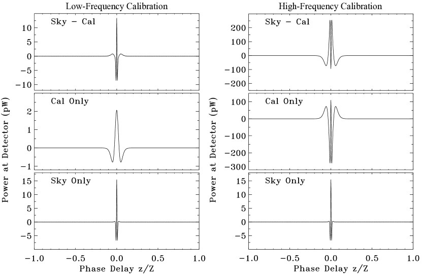
Figure 7: Simulated fringe patterns for different sky / calibrator combinations as the instrument views the median sky. The top panels show the fringe pattern observed when the calibrator covers one port while the other port views the sky. Center panels show the calibrator-only fringe pattern produced by summing the signals over two adjacent calibration passes ($\S$2.2). Bottom panels show the sky-only fringe pattern from subtracting adjacent passes. The left panels show the low-frequency calibration with the entire calibrator maintained 5 mK above the CMB monopole. The right panels show the high-frequency calibration when the single cavity is heated to 20 K. The detector noise in each plot is less than the line thickness.

Figure 7 shows a typical set of fringe patterns during calibration. We simulate the fringe pattern including continuum emission from the CMB, Galactic synchrotron, free-free, thermal dust, and the extragalactic contribution from the cosmic infrared background, to which we add line emission from the bright Cii ${}^{2}P_{3/2}\rightarrow~{}^{2}P_{1/2}$ fine-structure line at 157.74 $\mu$m rest wavelength. We model synchrotron emission as a power-law $I(\nu)\propto\nu^{\beta_{s}}$ with spectral index $\beta_{s}=-1.05$, and model free-free emission as a similar power law with spectral index $\beta_{ff}=-0.16$. We model thermal dust using a modified blackbody spectrum $I_{d}\propto B_{\nu}(T_{d})\nu^{\beta_{d}}$ with dust temperature $T_{d}=19.6$ K and spectral index $\beta_{d}=1.6$. The synchrotron, free-free, and dust amplitudes are normalized to the median brightness observed by Planck[26]. We model the extragalactic infrared background as a modified blackbody $I_{\rm CIB}\propto B_{\nu}(T_{\rm CIB})\nu^{\beta_{\rm CIB}}$ with $T_{\rm CIB}=18.5$ K, $\beta_{\rm CIB}=1.3$ and amplitude normalization from FIRAS[27]. The Cii normalization is set to 50% of the median dust foreground evaluated at the Cii rest frequency.

When viewing the median sky with the calibrator maintained 5 mK above the CMB monopole, the sampled fringe pattern peaks at amplitude $\sim$15 pW. Summing signals from adjacent scans with the calibrator at the CMB temperature vs 5 mK warmer cancels the sky signal ($\S$2.2), leaving just fringe pattern from the 5 mK calibrator difference. Similarly, subtracting signals from adjacent scans leaves just the sky signal (minus the calibrator monopole and 5 mK difference signal). The sharper peak in the sky-only signal compared to the calibrator-only signal results from diffuse dust emission, while the smaller high-frequency ripples in the sky signal result from line emission. To calibrate emission at frequencies above the CMB Wien cutoff, the single cavity in the calibrator is heated while the main calibrator body is cooled. The right panels in Figure 7 show the resulting high-frequency calibration. Note that the summed calibrator-only signal now contains sharply-peaked features typical of higher-frequency continuum sources.

Table 1: Simulated Total Power and Fringe Amplitude

Calibrator	Cavity	Total	Fringe
Temperature	Temperature	Power	Amplitude
(K)	(K)	(pW)	(pW)
Median Sky
2.725	2.725	585	15
2.730	2.730	587	13
2.720	2.720	583	18
2.000	20.000	695	94
2.500	2.500	503	98
3.000	3.000	716	116
Galactic Plane
2.725	2.725	1400	829
2.730	2.730	1400	827
2.720	2.720	1400	831
2.000	20.000	1510	719
2.500	2.500	1320	911
3.000	3.000	1530	698
Galactic Center
2.725	2.725	4920	4350
2.730	2.730	4920	4350
2.720	2.720	4920	4350
2.000	20.000	5030	4240
2.500	2.500	4840	4430
3.000	3.000	5050	4220

Table 1 compares the total (unmodulated) power at the detector to the largest (modulated) fringe amplitude for a selection of calibrator temperatures at three representative sky regions: the median sky brightness, the median Galactic plane ($|b|<1{{}^{\circ}}$), and the brightest sky (Galactic center). The principal science objectives observe the high-latitude sky with the entire calibrator within 5 mK of the CMB monopole. As the calibrator temperature changes, the peak fringe amplitude varies by 30% while the total power varies by 0.7%. Photon noise at the detectors produces noise equivalent power 2–3 $\times 10^{-16}$ W Hz^-1/2 depending on the high-frequency rolloff of emission from dust and zodiacal light. Assuming detector sampling at 256 Hz, each time-ordered sample has white noise with amplitude 5–7$\times 10^{-15}$ W. Cosmological signals of interest (Fig. 1) are small compared to the sampled noise and require integration over a large number of samples. Assuming that the telemetry digitization is set so that the noise exercises 2-3 bits, the fringe amplitudes from the median sky require 12–14 bits of dynamic range. Brighter emission from the Galactic plane or Galactic center require additional bits or lower post-detection gain. Since the photon noise is also significantly higher for these bright regions, a post-detection gain reduction can be employed to fully sample the fringe pattern from these pixels while remaining within 16 bit digitization.

Note that the sampled fringe patterns simplify data compression. Fringe amplitudes larger than 5 bits occur only near zero phase delay or at large sky/calibrator differences. Roughly 95% of the observations during flight will sample fringe amplitudes below 5 bits: the remaining 11 bits are identically zero to allow a compression factor of order 70%. The PIXIE data rate will thus be close to 6 kbps.

Figure 8: The fractional uncertainty in the PIXIE calibration varies with frequency. The solid line shows the combined fractional uncertainty in the calibration. The dotted and dashed lines show the spectral shape for CMB anisotropy and the combined foreground emission, respectively. In-flight calibration is expected to be accurate to a few parts in $10^{6}$ at frequencies dominated by the CMB, and a few parts in $10^{4}$ at higher frequencies dominated by the diffuse dust foreground.

6 Discussion

A blackbody calibrator has three major performance requirements. It must be sufficiently black and cover enough of the beam to reduce reflections and leakage to negligible levels. It must be sufficiently isothermal to reduce residual thermal gradients to negligible levels. The mean temperature must be determined with sufficient accuracy that temperature errors do not propagate to the final results. With these three conditions, the calibrator can be treated as a single source whose emission is completely determined by the temperature.

The PIXIE calibrator meets these conditions. The calibrator can be deployed to completely block either of the two exit apertures; the estimated leakage of -70 dB produces a calibration error less than $10^{-8}$. Both the calibrator and the instrument optics are maintained within 5 mK of CMB monopole temperature to minimize systematic errors in the calibration. Reflections at levels -65 dB terminate within the instrument blackbody cavity to create calibration error less than $10^{-8}$. Near-isothermal operation minimizes heat flow which could source thermal gradients; the predicted gradient during normal operation is less than 1 nK and would be undetectably small. Complementary data allow in-flight calibration of both the temperature and frequency scales to higher precision and accuracy than possible during pre-flight testing. Observations of bright Galactic lines determine the frequency scale to 200 Hz accuracy, well below the $\sim$15 GHz width of the synthesized frequency channels. Measurements of the Wien displacement in the peak of the blackbody calibrator spectra fix the absolute thermometry to 10 $\mu$K accuracy over the full range of commanded temperatures.

The PIXIE calibration is peformed in situ using the same data as the sky measurements: there are not separate calibration vs sky data sets and thus no systematic differences between calibration and sky data. Changing the calibrator temperature by a few mK provides an absolute reference signal at signal to noise ratio above $10^{3}$ on time scales of a few seconds and $10^{7}$ averaged over the full mission. Figure 8 shows the frequency dependence of the PIXIE calibration uncertainty. At frequencies below the CMB Wien cutoff, the calibration is expected to be accurate to a few parts in $10^{6}$, limited by the 10 $\mu$K uncertainty in the absolute temperature of the calibrator. At higher frequencies where the diffuse dust foreground dominates, thermal gradients within the calibrator produced when the single cavity is heated to 20 K limit the accuracy to a few parts in $10^{4}$. Other effects are negligible. The expected calibration accuracy is well under the requirements to detect the predicted $y$ and $\mu$ spectral distortions, which are the most stringent requirements of the PIXIE science goals.

References

- [1] D. H. D. H. Lyth and A. A. Riotto, Particle physics models of inflation and the cosmological density perturbation, Physics Reports 314 (1999) 1 [hep-ph/9807278].
- [2] L. M. Krauss and F. Wilczek, From B-modes to quantum gravity and unification of forces, International Journal of Modern Physics D 23 (2014) 1441001 [1404.0634].
- [3] L. M. Krauss and F. Wilczek, Using cosmology to establish the quantization of gravity, Physical Review D 89 (2014) 047501 [1309.5343].
- [4] J. Chluba, A. Kogut, S. P. Patil, M. H. Abitbol, N. Aghanim, Y. Ali-Haımoud et al., Spectral Distortions of the CMB as a Probe of Inflation, Recombination, Structure Formation and Particle Physics, Bulletin of the American Astronomical Society 51 (2019) 184 [1903.04218].
- [5] BICEP2 Collaboration and Keck Array Collaboration, Improved Constraints on Cosmology and Foregrounds from BICEP2 and Keck Array Cosmic Microwave Background Data with Inclusion of 95 GHz Band, Physical Review Letters 116 (2016) 031302 [1510.09217].
- [6] Y. B. Zeldovich and R. A. Sunyaev, The Interaction of Matter and Radiation in a Hot-Model Universe, Astrophysics and Space Science 4 (1969) 301.
- [7] R. A. Sunyaev and Y. B. Zeldovich, The interaction of matter and radiation in the hot model of the Universe, II, Astrophysics and Space Science 7 (1970) 20.
- [8] D. J. Fixsen, E. S. Cheng, J. M. Gales, J. C. Mather, R. A. Shafer and E. L. Wright, The Cosmic Microwave Background Spectrum from the Full COBE FIRAS Data Set, The Astrophysical Journal 473 (1996) 576 [astro-ph/9605054].
- [9] A. Kogut, M. H. Abitbol, J. Chluba, J. Delabrouille, D. Fixsen, J. C. Hill et al., CMB Spectral Distortions: Status and Prospects, in Bulletin of the American Astronomical Society, vol. 51, p. 113, Sept., 2019, 1907.13195.
- [10] D. J. Fixsen, E. S. Cheng, D. A. Cottingham, J. Eplee, R. E., T. Hewagama, R. B. Isaacman et al., Calibration of the COBE FIRAS Instrument, The Astrophysical Journal 420 (1994) 457.
- [11] C. L. Bennett, G. F. Smoot, M. Janssen, S. Gulkis, A. Kogut, G. Hinshaw et al., COBE Differential Microwave Radiometers: Calibration Techniques, The Astrophysical Journal 391 (1992) 466.
- [12] J. L. Weiland, N. Odegard, R. S. Hill, E. Wollack, G. Hinshaw, M. R. Greason et al., Seven-year Wilkinson Microwave Anisotropy Probe (WMAP) Observations: Planets and Celestial Calibration Sources, The Astrophysical Journal Supplement Series 192 (2011) 19 [1001.4731].
- [13] Planck Collaboration, P. A. R. Ade, N. Aghanim, C. Armitage-Caplan, M. Arnaud, M. Ashdown et al., Planck 2013 results. VIII. HFI photometric calibration and mapmaking, Astronomy and Astrophysics 571 (2014) A8 [1303.5069].
- [14] G. Hinshaw, C. Barnes, C. L. Bennett, M. R. Greason, M. Halpern, R. S. Hill et al., First-Year Wilkinson Microwave Anisotropy Probe (WMAP) Observations: Data Processing Methods and Systematic Error Limits, The Astrophysical Journal Supplement Series 148 (2003) 63 [astro-ph/0302222].
- [15] Planck Collaboration, N. Aghanim, C. Armitage-Caplan, M. Arnaud, M. Ashdown, F. Atrio-Barandela et al., Planck 2013 results. V. LFI calibration, Astronomy and Astrophysics 571 (2014) A5 [1303.5066].
- [16] A. Kogut, D. J. Fixsen, D. T. Chuss, J. Dotson, E. Dwek, M. Halpern et al., The Primordial Inflation Explorer (PIXIE): a nulling polarimeter for cosmic microwave background observations, Journal of Cosmology and Astroparticle Physics 7 (2011) 25 [1105.2044].
- [17] N. W. Boggess, J. C. Mather, R. Weiss, C. L. Bennett, E. S. Cheng, E. Dwek et al., The COBE Mission: Its Design and Performance Two Years after Launch, The Astrophysical Journal 397 (1992) 420.
- [18] Z. Pan, M. Liu, R. Basu Thakur, B. A. Benson, D. J. Fixsen, H. Goksu et al., Compact millimeter-wavelength Fourier-transform spectrometer, Applied Optics 58 (2019) 6257 [1905.07399].
- [19] D. J. Fixsen, E. J. Wollack, A. Kogut, M. Limon, P. Mirel, J. Singal et al., Compact radiometric microwave calibrator, Review of Scientific Instruments 77 (2006) 064905.
- [20] E. J. Wollack, D. J. Fixsen, R. Henry, A. Kogut, M. Limon and P. Mirel, Electromagnetic and Thermal Properties of a Conductively Loaded Epoxy, International Journal of Infrared and Millimeter Waves 29 (2008) 51.
- [21] P. C. Nagler, D. J. Fixsen, A. Kogut and G. S. Tucker, Systematic Effects in Polarizing Fourier Transform Spectrometers for Cosmic Microwave Background Observations, The Astrophysical Journal Supplement Series 221 (2015) 21 [1510.08089].
- [22] D. J. Fixsen, A. Kogut, S. Levin, M. Limon, P. Lubin, P. Mirel et al., ARCADE 2 Measurement of the Absolute Sky Brightness at 3-90 GHz, The Astrophysical Journal 734 (2011) 5 [0901.0555].
- [23] A. J. Kogut and D. J. Fixsen, Systematic error cancellation for a four-port interferometric polarimeter, Journal of Astronomical Telescopes, Instruments, and Systems 5 (2019) 024008 [1908.00558].
- [24] D. J. Fixsen, The Temperature of the Cosmic Microwave Background, The Astrophysical Journal 707 (2009) 916 [0911.1955].
- [25] J. L. Pineda, W. D. Langer, T. Velusamy and P. F. Goldsmith, A Herschel [C ii] Galactic plane survey. I. The global distribution of ISM gas components, Astronomy and Astrophysics 554 (2013) A103 [1304.7770].
- [26] Planck Collaboration, Y. Akrami, M. Ashdown, J. Aumont, C. Baccigalupi, M. Ballardini et al., Planck 2018 results. IV. Diffuse component separation, arXiv e-prints (2018) arXiv:1807.06208 [1807.06208].
- [27] D. J. Fixsen, E. Dwek, J. C. Mather, C. L. Bennett and R. A. Shafer, The Spectrum of the Extragalactic Far-Infrared Background from the COBE FIRAS Observations, The Astrophysical Journal 508 (1998) 123 [astro-ph/9803021].