Off-axis optical vortices using double-Raman singlet and doublet light-matter schemes

Abstract

We study the formation of off-axis optical vortices propagating inside a double-Raman gain atomic medium. The atoms interact with two weak probe fields as well as two strong pump beams which can carry orbital angular momentum (OAM). We consider a situation when only one of the strong pump lasers carries an OAM. A particular superposition of probe fields coupled to the matter is shown to form specific optical vortices with shifted axes. Such off-axis vortices can propagate inside the medium with sub- or superluminal group velocity depending on the value of the two-photon detuning. The superluminal optical vortices are associated with the amplification as the energy of pump fields is transferred to the probe fields. The position of the peripheral vortices can be manipulated by the OAM and intensity of the pump fields. We show that the exchange of optical vortices is possible between individual probe beams and the pump fields when the amplitude of the second probe field is zero at the beginning of the atomic cloud. The model is extended to a more complex double Raman doublet interacting with four pump fields. In contrast to the double-Raman-singlet, now the generation of the off-axis sub- or superluminal optical vortices is possible even for zero two-photon detuning.

I Introduction

Electromagnetically induced transparency (EIT) Harris (1997); Fleischhauer et al. (2005) is an optical effect in which the susceptibility of a weak probe field is modified for an optically thick three-level $\Lambda$ atomic system. The medium becomes transparent for the probe transition by applying a stronger control field driving another transition of the $\Lambda$ system. A number of important phenomena Paspalakis et al. (2002); Paspalakis and Kis (2002a, b); Ruseckas et al. (2007) rely on the EIT, including adiabatons Grobe et al. (1994); Fleischhauer and Manka (1996); Wang et al. (2001), matched pulses Harris (1994); Cerboneschi and Arimondo (1995), giant optical nonlinearities Harris et al. (1990); Deng et al. (1998); Wang et al. (2001); Kang and Zhu (2003); Hamedi and Juzeliūnas (2015) and optical solitons Wu and Deng (2004a, b). Due to the EIT the light pulses can be slowed down Harris (1997); Hau et al. (1999); Lukin (2003); Juzeliūnas and Öhberg (2004); Fleischhauer et al. (2005); Ruseckas et al. (2011a); Bao et al. (2011); Ruseckas et al. (2013); Lee et al. (2014) and also stored in the atomic medium by switching off the controlled laser Phillips et al. (2001); Liu et al. (2001); Lukin and Imamoglu (2001); Juzeliūnas and Carmichael (2002); Lukin (2003). This can be used to store the quantum state of light to the matter and back to the light leading to important applications in quantum technologies Lukin (2003); Ma et al. (2017); Hsiao et al. (2018).

In parallel, there have been important efforts dedicated to the superluminal propagation of light pulses in coherently driven atomic media Jiang et al. (2007); M.Mahmoudi et al. (2006); qi Kuang et al. (2009); Akulshin and McLean (2010). An anomalous dispersion leading to the superluminal propagation can be naturally obtained within the absorption band medium Chu and Wong (1982) or inside a tunnel barrier Steinberg et al. (1993). Yet such a superluminal propagation is hardly observed due to losses Chu and Wong (1982). Some novel approaches have been proposed to utilize transparent spectral regions for fast light Chiao (1993); Dogariu et al. (2001); Glasser et al. (2012); Bianucci et al. (2008); Kudriašov et al. (2014). Specifically, it was shown that a linear anomalous dispersion can be created in a Raman gain doublet and therefore distorsionless pulse propagation is possible Dogariu et al. (2001).

Vortex beams of light Allen et al. (1999); Padgett et al. (2004); Babiker et al. (2018) representing an example of the singular optics, are of the fundamental interest and offer many applications Babiker et al. (1994); Molina-Terriza et al. (2001); Pugatch et al. (2007); Dutton and Ruostekoski (2004); Bishop et al. (2004); Ruseckas et al. (2007); Chen et al. (2008); Lembessis and Babiker (2010); Ruseckas et al. (2011b); Ding et al. (2012); Walker et al. (2012); Ruseckas et al. (2013); Lembessis et al. (2014); Radwell et al. (2015); Sharma and Dey (2017); Hamedi et al. (2018a, b, 2019a); Moretti et al. (2009); Cardano et al. (2015); Hamedi et al. (2019b); Hong et al. (2019); Qiu et al. (2020). The optical vortices are described by a wave field whose phase advances around the axis of the vortex, and the associated wavefront carries an orbital angular momentum (OAM) Allen et al. (1999); Padgett et al. (2004); Babiker et al. (2018). The phase of the on-axis optical vortices advances linearly and monotonically with the azimuthal coordinate reaching a multiple of $2\pi$ after completing a closed circle around the beam axis. When two twisted beams each carrying an optical vortex are superimposed, the resulting beam contains new vortices depending on the charge of each vortex component Maleev and Swartzlander (2003); Galvez et al. (2006); Baumann et al. (2009); Hamedi et al. (2019a). Besides the on-axis vortices, the off-axis optical vortices can be formed for which the vortex core is not on the beam axis but moves about it Mair et al. (2001); Basistiy et al. (2003); Lee et al. (2005); Baumann et al. (2009); Wang (2017).

In this article we propose a scenario for formation of off-axis optical vortices in a four-level atom-light coupling scheme. We consider a double-Raman gain medium interacting with two weak probe fields, as well as two stronger pump laser beams which can carry the OAM. A specific combination of the probe fields is formed with a definite group velocity determined by the two-photon detuning. Note that the individual probe beams do not have a definite group velocity when propagating inside the medium. If one of the pump laser beams carries an optical vortex, the resulting superposition beam exhibits off-axis vortices propagating inside the medium with a sub- or superluminal group velocity depending on the two-photon detuning. The position of the peripheral vortices around the center can be manipulated by the OAM and the intensity of the pump fields. It is shown analytically and numerically that the OAM of the pump fields can be transferred to the individual probe beams when the amplitude of the second probe field is zero at the beginning of the medium. We also extend the model to a more complex double Raman doublet scheme interacting with four pump fields.

The paper is organized as follows. In the next Section we consider the light propagation using a double Raman scheme and show that off-axis optical vortices with either slow or fast light properties can be created. In Section III we extend the model by considering formation of the off-axis optical vortices occurring under the slow or fast light propagation in the double Raman doublet scheme. Our results are summarized in Section IV.

II The double-Raman scheme

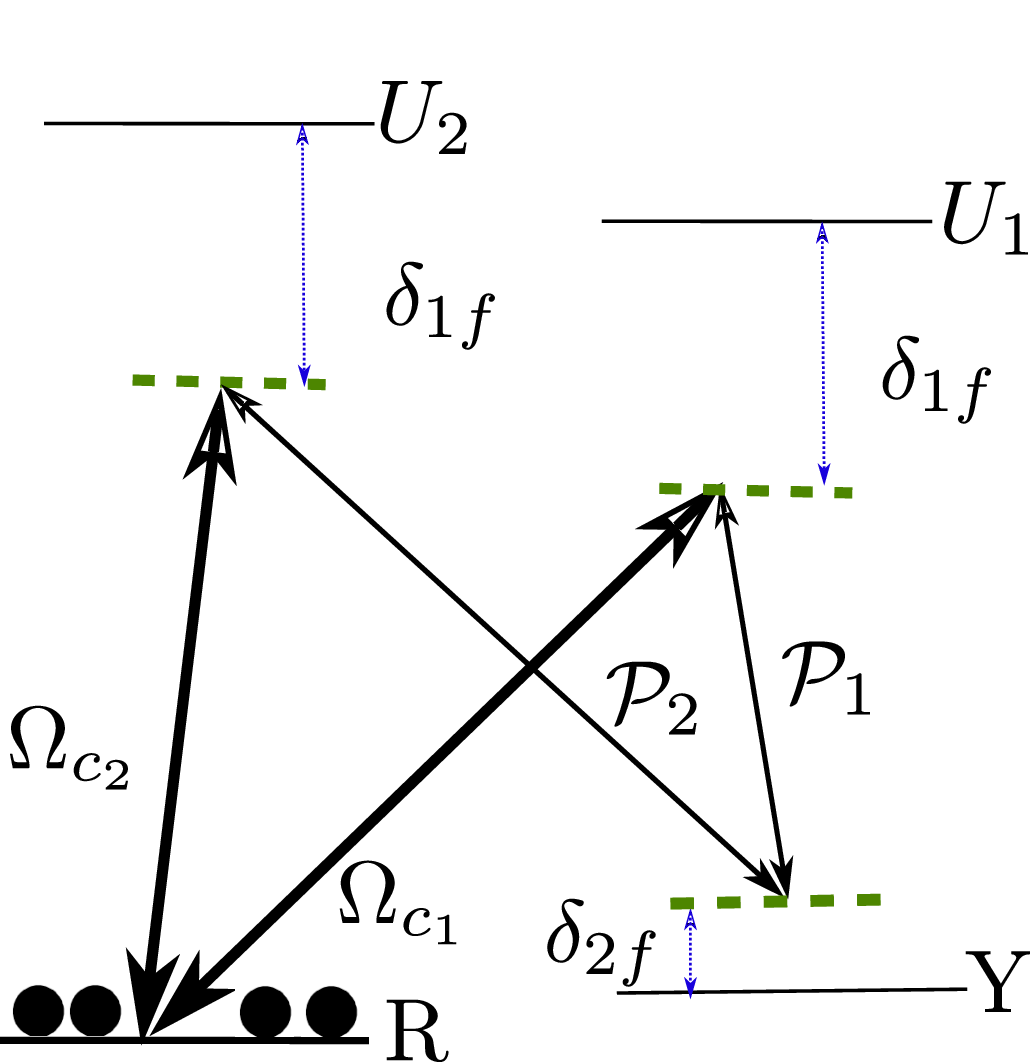
Figure 1: Schematic diagram of the double Raman scheme

Let us consider propagation of two probe fields in an atomic medium with the Raman gain described by the double Raman scheme illustrated in Fig. 1. The atoms forming the medium are characterized by two hyperfine ground levels $R$ and $Y$ and two electronic excited levels $U_{1}$ and $U_{2}$. The quantum state of the atoms is described by the probability amplitudes $\textbf{$\Psi_{R}$}(\textbf{r},t)$, $\textbf{$\Psi_{Y}$}(\textbf{r},t)$, $\textbf{$\Psi_{U_{1}}$}(\textbf{r},t)$, and $\textbf{$\Psi_{U_{2}}$}(\textbf{r},t)$ normalized to the atomic density $n$: $|\textbf{$\Psi_{R}$}|^{2}+|\textbf{$\Psi_{Y}$}|^{2}+|\textbf{$\Psi_{U_{1}}$}|^{2}+|\textbf{$\Psi_{U_{2}}$}|^{2}=n$.

The atoms interact with two weak probe fields with slowly varying amplitudes $\mathcal{P}_{1}$ and $\mathcal{P}_{2}$, as well as two strong pump lasers. The Rabi frequencies of the pump fields can be generally expressed as

$$\Omega_{c_{j}}=\mathcal{E}_{c_{j}}(r)e^{il_{j}\varphi},$$ (1)

where

$$\mathcal{E}_{c_{j}}(r)=|\Omega_{c_{j}}|(r/w)^{|l_{j}|}e^{-r^{2}/w^{2}},$$ (2)

is a fundamental Gaussian beam for $l_{j}=0$, while it describes a Laguerre-Gaussian (LG) doughnut beam when $l_{j}\neq 0$. Here $\varphi$ is the azimuthal angle, $r$ describes the cylindrical radius, $w$ denotes the beam waist parameter, and $|\Omega_{c_{j}}|$ ($j=1,2$) is the strength of the pump beam.

The atoms are assumed to be initially in the ground level (Raman level) $R$. The Rabi frequency and duration of the probe pulses are small enough, so that the depletion of the ground level $R$ is neglected. We work under the four-photon resonance condition $\omega_{p_{1}}-\omega_{c_{1}}=\omega_{p_{2}}-\omega_{c_{2}}$, where $\omega_{p_{1}}$ and $\omega_{p_{2}}$ are the frequencies of the probe beams, and $\omega_{c_{1}}$ and $\omega_{c_{2}}$ are the frequencies of the pump beams.

After introducing the slowly varying atomic amplitudes we obtain the following equations for slowly varying probe fields

$$(\partial_{t}+c\partial_{z})\mathcal{P}_{1} =i\alpha_{1}\Phi_{Y}^{*}\Phi_{U_{1}},$$ (3)

$$(\partial_{t}+c\partial_{z})\mathcal{P}_{2} =i\alpha_{2}\Phi_{Y}^{*}\Phi_{U_{2}},$$ (4)

where $\alpha_{1}=\mu_{1}\sqrt{\omega_{p_{1}}/2\varepsilon_{0}\hbar}$, $\alpha_{2}=\mu_{2}\sqrt{\omega_{p_{2}}/2\varepsilon_{0}\hbar}$ denote the coupling strength of the probe beams with the atoms, while $\mu_{1}$ and $\mu_{2}$ represent the dipole moments for the corresponding atomic transitions. It should be noted that the diffraction terms containing the transverse derivatives have been neglected in the Maxwell equations (3) and (4). These terms are negligible if the phase change of the probe fields due to these terms is much smaller than $\pi$ Ruseckas et al. (2013); Hamedi et al. (2018b, 2019a).

Assuming that the strength of the coupling of the probe fields with the atoms is the same $\alpha_{1}=\alpha_{2}=\alpha$, one arrives at the following equations for the slowly varying atomic amplitudes

$$i\partial_{t}\Phi_{U_{1}} =\delta_{1f}\Phi_{U_{1}}-\alpha\mathcal{P}_{1}\Phi_{Y}-\mathcal{E}_{c_{1}}(r)e^{il_{1}\varphi}\Phi_{R},$$ (5)

$$i\partial_{t}\Phi_{U_{2}} =\delta_{1f}\Phi_{U_{2}}-\alpha\mathcal{P}_{2}\Phi_{Y}-\mathcal{E}_{c_{2}}(r)e^{il_{2}\varphi}\Phi_{R},$$ (6)

$$i\partial_{t}\Phi_{Y} =(\delta_{2f}-i\Gamma)\Phi_{Y}-\alpha\mathcal{P}_{1}^{*}\Phi_{U_{1}}-\alpha\mathcal{P}_{2}^{*}\Phi_{U_{2}},$$ (7)

where $\delta_{1f}=\omega_{U_{1}}-\omega_{R}-\omega_{c_{1}}=\omega_{U_{2}}-\omega_{R}-\omega_{c_{2}}$ describes the one-photon detuning, $\delta_{2f}=\omega_{p_{1}}-\omega_{c_{1}}+\omega_{Y}-\omega_{R}=\omega_{p_{2}}-\omega_{c_{2}}+\omega_{Y}-\omega_{R}$ represents the two-photon detuning and $\Gamma$ is the decay rate of the level $Y$. Here, $\omega_{U_{1}}$, $\omega_{U_{2}}$ , and $\omega_{Y}$ are energies of the atomic states $U_{1}$, $U_{2}$ and $Y$, respectively.

We consider the case of monochromatic probe beams with the time-independent amplitudes $\mathcal{P}_{1}$ and $\mathcal{P}_{2}$ and the spatially homogeneous atomic amplitudes $\Phi_{R}$, $\Phi_{Y}$, $\Phi_{U_{1}}$, and $\Phi_{U_{2}}$. We will look for the stationary solutions characterized by the time-independent atomic amplitudes $\Phi_{R}$, $\Phi_{Y}$, $\Phi_{U_{1}}$, and $\Phi_{U_{2}}$, giving

$$c\partial_{z}\mathcal{P}_{1}-i\alpha\Phi_{Y}^{*}\Phi_{U_{1}} =0,$$ (8)

$$c\partial_{z}\mathcal{P}_{2}-i\alpha\Phi_{Y}^{*}\Phi_{U_{2}} =0,$$ (9)

$$\delta_{1f}\Phi_{U_{1}}-\alpha\mathcal{P}_{1}\Phi_{Y}-\mathcal{E}_{c_{1}}(r)e^{il_{1}\varphi}\Phi_{R} =0,$$ (10)

$$\delta_{1f}\Phi_{U_{2}}-\alpha\mathcal{P}_{2}\Phi_{Y}-\mathcal{E}_{c_{2}}(r)e^{il_{2}\varphi}\Phi_{R} =0,$$ (11)

$$(\delta_{2f}-i\Gamma)\Phi_{Y}-\alpha\mathcal{P}_{1}^{*}\Phi_{U_{1}}-\alpha\mathcal{P}_{2}^{*}\Phi_{U_{2}} =0.$$ (12)

For a large one-photon detuning $\delta_{1f}$ ($\delta_{1f}|\delta_{2f}-i\gamma|\gg\alpha^{2}|\mathcal{P}_{1,2}|^{2}$), Eqs. (10) and (11) give

$$\Phi_{U_{1}} =\frac{\mathcal{E}_{c_{1}}(r)}{\delta_{1f}}e^{il_{1}\varphi}\Phi_{R},$$ (13)

$$\Phi_{U_{2}} =\frac{\mathcal{E}_{c_{2}}(r)}{\delta_{1f}}e^{il_{2}\varphi}\Phi_{R}.$$ (14)

Substituting Eqs. (13) and (14) into Eq. (12) yields

$$\Phi_{Y}=\frac{\alpha\Phi_{R}}{\delta_{1f}(\delta_{2f}-i\Gamma)}\left(\mathcal{E}_{c_{1}}(r)e^{il_{1}\varphi}\mathcal{P}_{1}^{*}+\mathcal{E}_{c_{2}}(r)e^{il_{2}\varphi}\mathcal{P}_{2}^{*}\right).$$ (15)

Using Eqs. (13)-(15) the propagation equation for both probe fields $P_{1}$ and $P_{2}$ (Eqs. (8) and (9)) take the form

$$\partial_{z}P_{1}-i\beta\left(\frac{|\mathcal{E}_{c_{1}}(r)|^{2}\mathcal{P}_{1}+\mathcal{E}_{c_{1}}(r)\mathcal{E}_{c_{2}}^{*}(r)e^{i(l_{1}-l_{2})\varphi}\mathcal{P}_{2}}{(\delta_{2f}+i\Gamma)}\right) =0,$$ (16)

$$\partial_{z}P_{2}-i\beta\left(\frac{\mathcal{E}_{c_{1}}^{*}(r)\mathcal{E}_{c_{2}}(r)e^{i(l_{2}-l_{1})\varphi}\mathcal{P}_{1}+|\mathcal{E}_{c_{2}}(r)|^{2}\mathcal{P}_{2}}{(\delta_{2f}+i\Gamma)}\right) =0,$$ (17)

with

$$\beta=\frac{\alpha^{2}|\Phi_{R}|^{2}}{c\delta_{1f}^{2}}=\frac{\alpha^{2}n}{c\delta_{1f}^{2}}.$$ (18)

We now introduce new fields representing superpositions of the original probe beams

$$\psi=\frac{1}{\mathcal{E}_{c}(r)}\left(\mathcal{E}_{c_{1}}^{*}(r)e^{-il_{1}\varphi}\mathcal{P}_{1}+\mathcal{E}_{c_{2}}^{*}(r)e^{-il_{2}\varphi}\mathcal{P}_{2}\right),$$ (19)

$$\xi=\frac{1}{\mathcal{E}_{c}(r)}\left(\mathcal{E}_{c_{2}}(r)e^{il_{2}\varphi}\mathcal{P}_{1}-\mathcal{E}_{c_{1}}(r)e^{il_{1}\varphi}\mathcal{P}_{2}\right),$$ (20)

where

$$\mathcal{E}_{c}(r)=\sqrt{|\mathcal{E}_{c_{1}}(r)|^{2}+|\mathcal{E}_{c_{2}}(r)|^{2}}.$$ (21)

is the total strength of the control fields. Calling on Eqs. (19) and (20), one can rewrite Eqs. (16) and (17) as

$$\partial_{z}\psi-i\kappa\psi=0,$$ (22)

$$\partial_{z}\xi=0,$$ (23)

where

$$\kappa=\beta\frac{\mathcal{E}_{c}^{2}(r)}{(\delta_{2f}+i\Gamma)}.$$ (24)

This behavior of the modes $\psi$ and $\xi$ is similar to propagation in double-lambda system. Eqs. (22) and (23) clearly show that one of the superposition fields $\psi$ interacts with the atoms while another field $\xi$ does not interact and propagates as in the free space. The solution of Eq. (22) reads

$$\psi(z)=\frac{1}{\mathcal{E}_{c}(r)}\left(\mathcal{E}_{c_{1}}^{*}(r)e^{-il_{1}\varphi}\mathcal{P}_{1}(0)+\mathcal{E}_{c_{2}}^{*}(r)e^{-il_{2}\varphi}\mathcal{P}_{2}(0)\right)e^{i\frac{\Gamma}{\delta_{1f}^{2}}\frac{\mathcal{E}_{c}^{2}(r)}{(\delta_{2f}+i\Gamma)}\frac{z}{L_{\Gamma}}},$$ (25)

where

$$L_{\Gamma}=\frac{\Gamma c}{n\alpha^{2}},$$ (26)

determines the characteristic length related to the decay of the excited level $Y$.

The group velocity of the light given by Eq. (25) can be calculated as

$$\nu_{g}=\frac{c}{1+\frac{\alpha^{2}n\mathcal{E}_{c}^{2}(r)}{\delta_{1f}^{2}}\frac{\Gamma^{2}-\delta_{2f}^{2}}{(\delta_{2f}^{2}+\Gamma^{2})^{2}}}.$$ (27)

Equation  (27) is very similar to group velocity in a Raman system with single probe beam. Clearly, when $\Gamma<\delta_{2f}$ the group velocity exceeds $c$ providing the superluminality. On the other hand, the slow light propagates in the medium when $\Gamma>\delta_{2f}$ ($\nu_{g}<c$ ). In particular, the superluminal propagation is associated with the amplification since the energy of pump fields is transferred to the probe fields. This can be easily seen from the fact that the coefficient $\kappa$ in Eq. (24) is a complex number.

In the following we consider a case where the first pump field $\Omega_{c_{1}}$ is a vortex $l_{1}\neq 0$, while the second pump field is a non-vortex Gaussian beam with $l_{2}=0$. We have made such an assumption to avoid the zero denominator when $r\rightarrow 0$ in Eq. (25) if $l_{2}\neq 0$. Numerical simulations presented in Figs. (2)-(7) show the superposition beam given by Eq. (25) in a transverse plane of the beam at $z=L_{\Gamma}$.

Figure 2 (4) displays the numerical results of the intensity distributions of the superposition beam $\psi$ when the two-photon detuning is larger (smaller) than $\Gamma$ corresponding to superluminal (subluminal) propagation of superposition pulse inside the medium, and for different vorticities $l_{1}=1-6$. Figure 3 (5) shows the corresponding helical phase patterns. For simulations we have selected $\delta_{2f}=4\Gamma$ and $\delta_{2f}=0$ corresponding to the superluminal and subluminal situations, respectively.

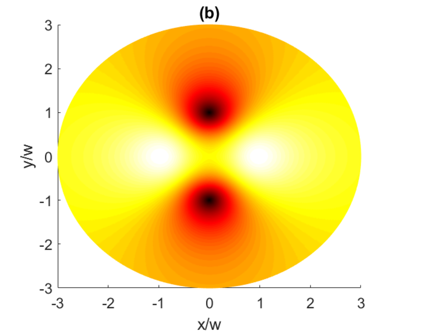
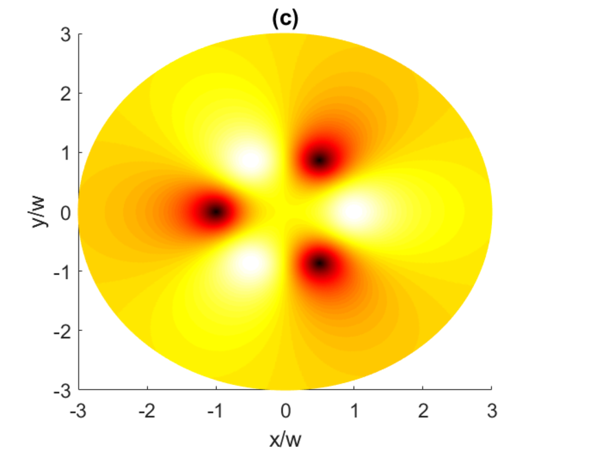
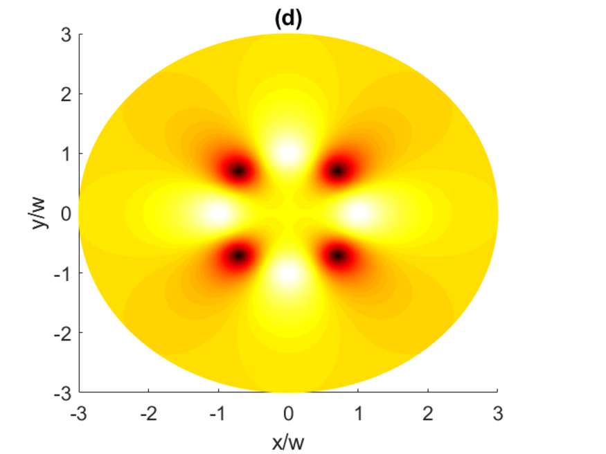
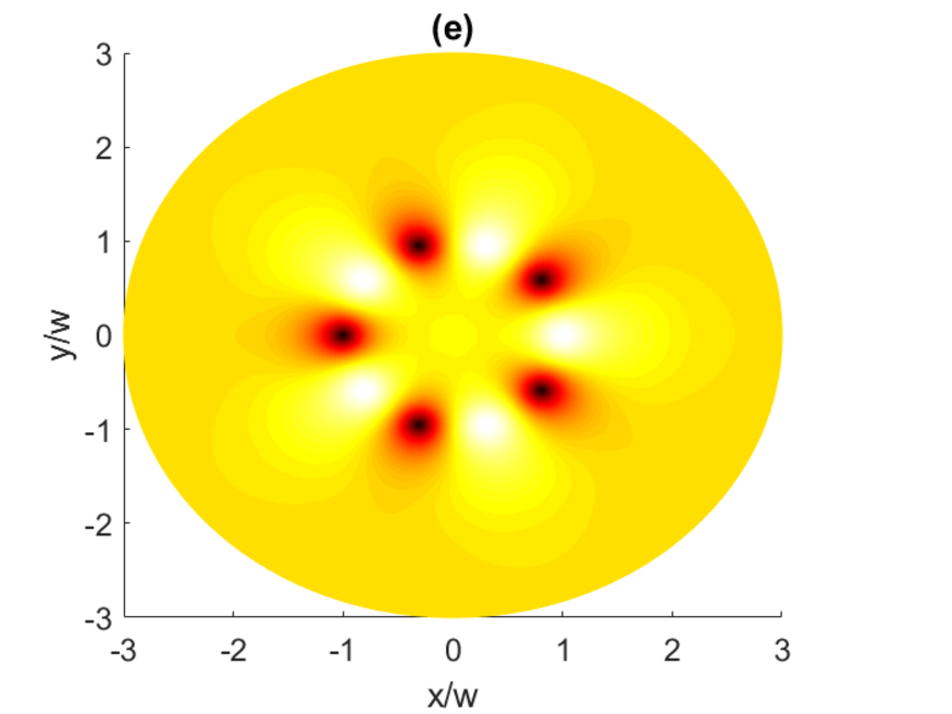
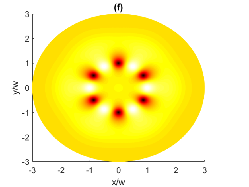
Figure 2: Intensity distributions (in arbitrary units) of the superluminal superposition beam $\psi$ featured in Eq. (25) with different vorticities $l_{1}=1-6$ (a)-(e). Here the parameters are $|\Omega_{c_{1}}|=|\Omega_{c_{2}}|=\Gamma$, $\delta_{1f}=\Gamma$, $z=L_{\Gamma}$, $l_{2}=0$ and $\delta_{2f}=4\Gamma$.

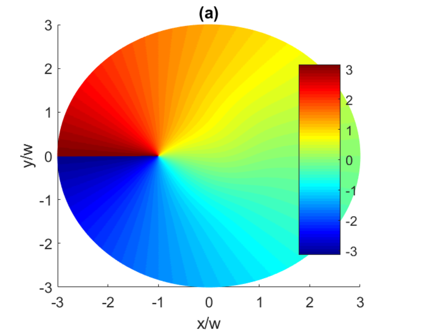
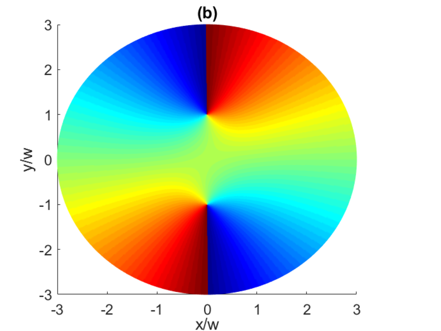
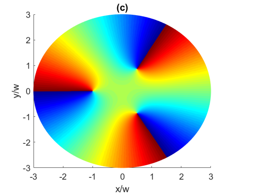
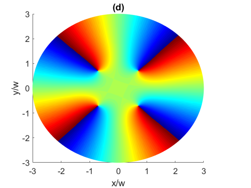
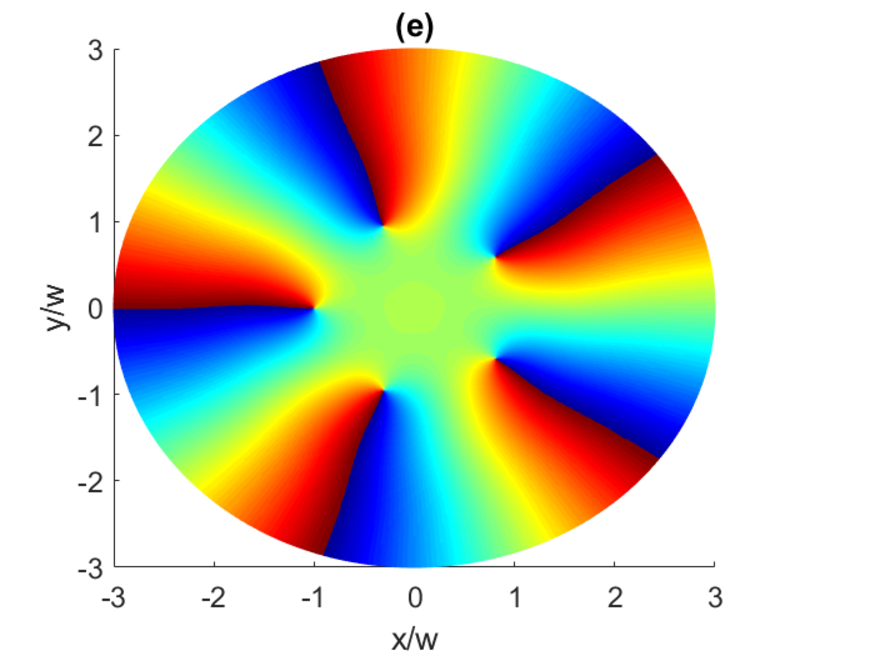
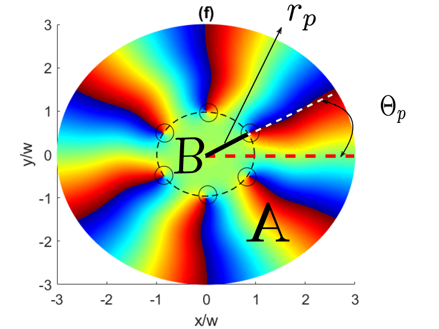
Figure 3: The helical phase patterns of the superluminal superposition beam $\psi$ featured in Eq. (25) with different vorticities $l_{1}=1-6$ (a)-(e). The parameters are taken to be the same as in Fig. 2.

The resulting beam is seen to have a very particular shape. The center of the superposition beam contains no vortex and is surrounded by $l_{1}$ singly charged peripheral vortices of sign $l_{1}/|l_{1}|$. The peripheral vortices are distributed at angles

$$\Theta_{p}=\frac{n\pi}{l_{1}},$$ (28)

with an approximate radial distance to the beam center

$$r_{p}\approx\left(|l_{1}|!\frac{|\Omega_{c_{2}}|}{|\Omega_{c_{1}}|}\right)^{\frac{1}{2|l_{1}|}},$$ (29)

where $n=1...2|l_{1}|$ is an integer for each peripheral vortex Baumann et al. (2009). The off-axis vortices are placed at the same radial distance from the core of the superposition beam.

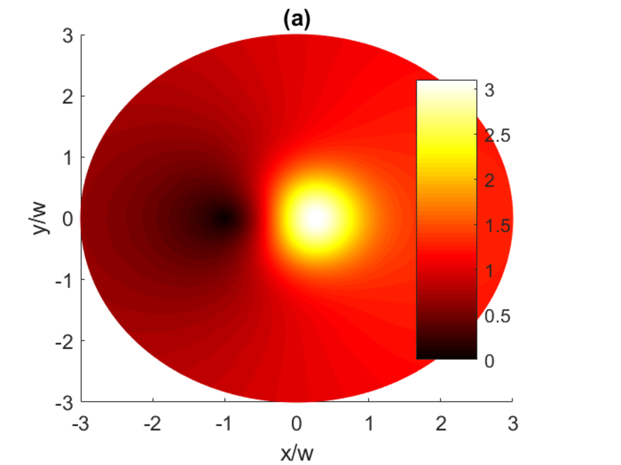
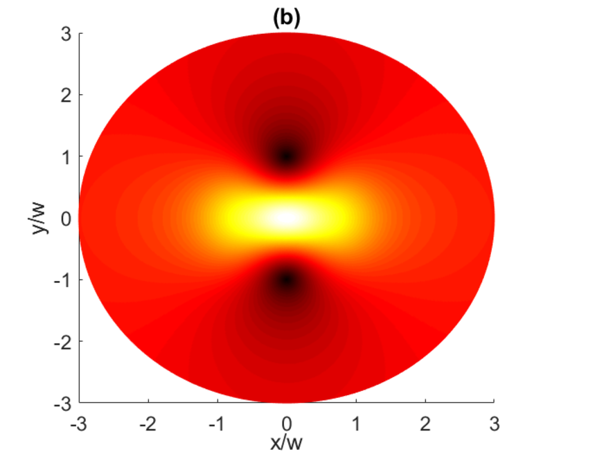
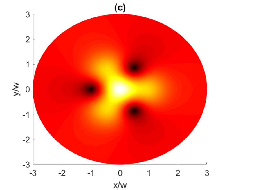
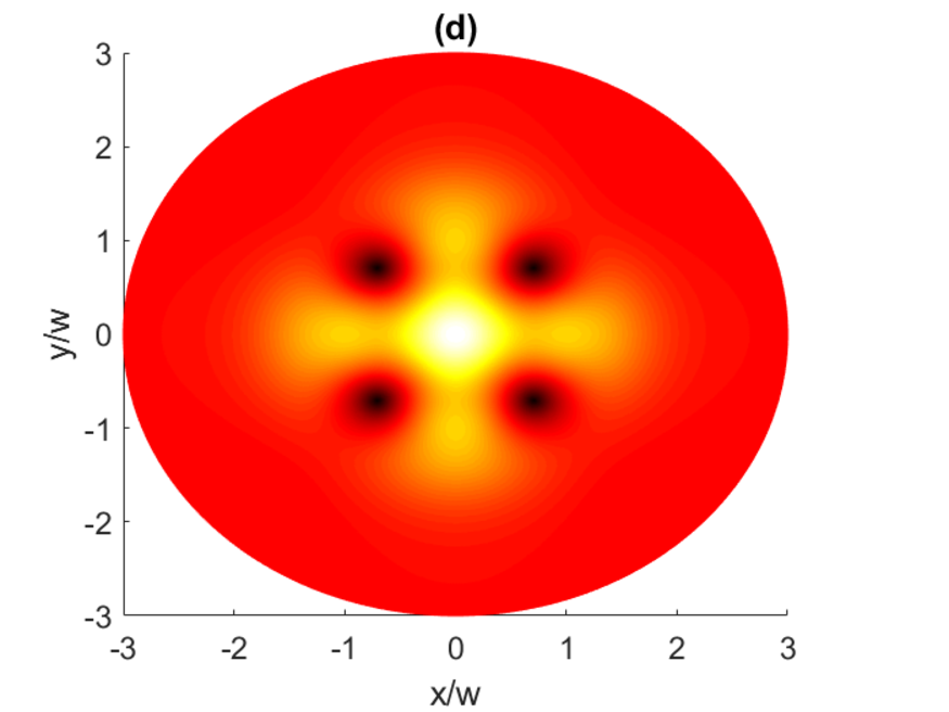
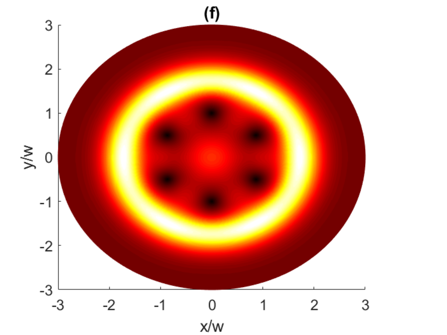
Figure 4: Intensity distributions (in arbitrary units) of the subluminal superposition beam $\psi$ featured in Eq. (25) with different vorticities $l_{1}=1-6$ (a)-(e). Here the parameters are $|\Omega_{c_{1}}|=|\Omega_{c_{2}}|=\Gamma$, $\delta_{1f}=\Gamma$, $z=L_{\Gamma}$ and $\delta_{2f}=0$.

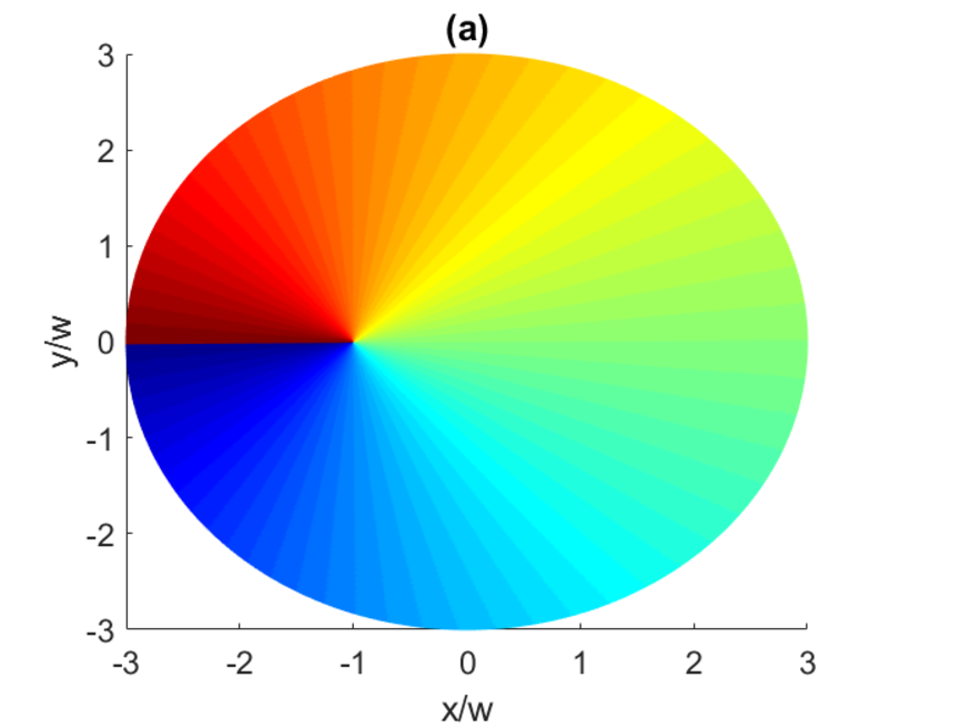
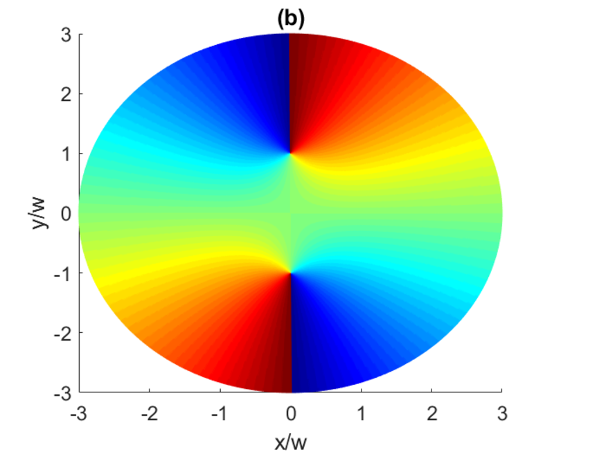
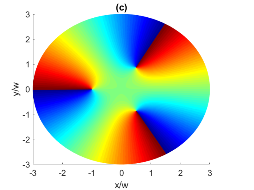
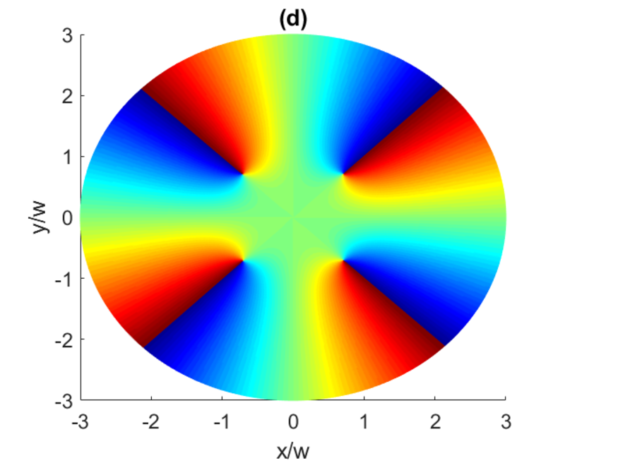
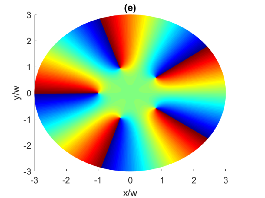
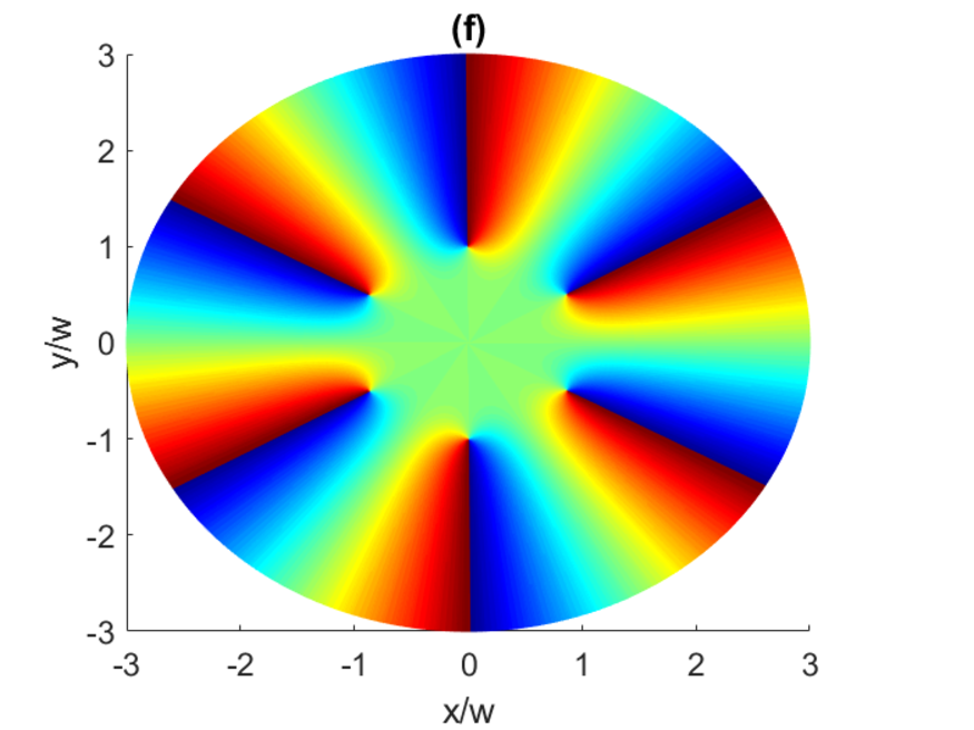
Figure 5: The helical phase patterns of the subluminal superposition beam $\psi$ featured in Eq. (25) with different vorticities $l_{1}=1-6$ (a)-(e). The parameters are the same as Fig. 4.

Such images of the subluminal or superluminal vortices appear as two initial pump beams with different azimuthal indices $l_{1}\neq 0$ and $l_{2}=0$ are superimposed leading to formation of the off-center vortices with shifted axes. To elucidate this better, let us consider Fig. 3(f) which is plotted for $l_{1}=6$. Note that we have considered a case where the strength of both coupling beams are the same ($|\Omega_{c_{1}}|=|\Omega_{c_{2}}|=\Gamma$). Region $A$ is dominated by the vortex beam with $\Omega_{c_{1}}$ and $l_{1}=6$, while the inner region $B$ is dominated by the Gaussian beam $\Omega_{c_{2}}$ with $l_{2}=0$. The peripheral vortices are located precisely at the boundary between the two regions which is a circle of the radius $r_{p}$.

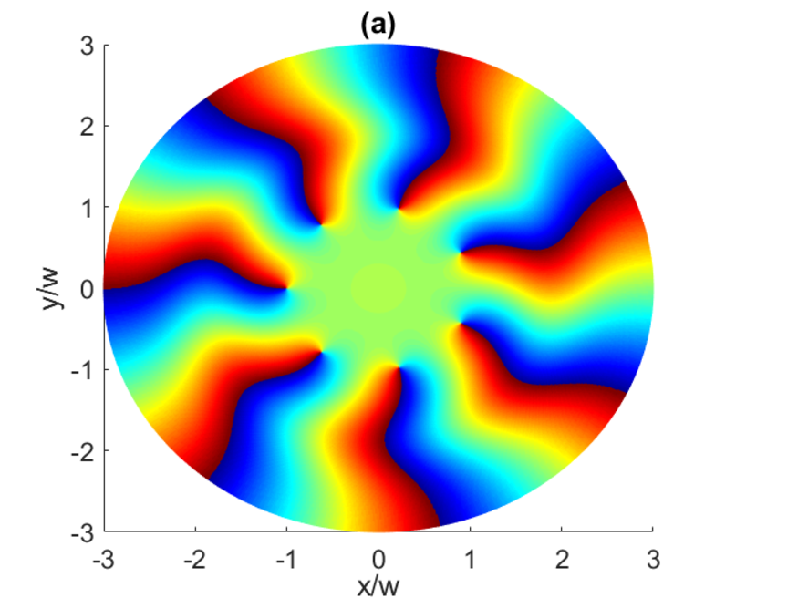
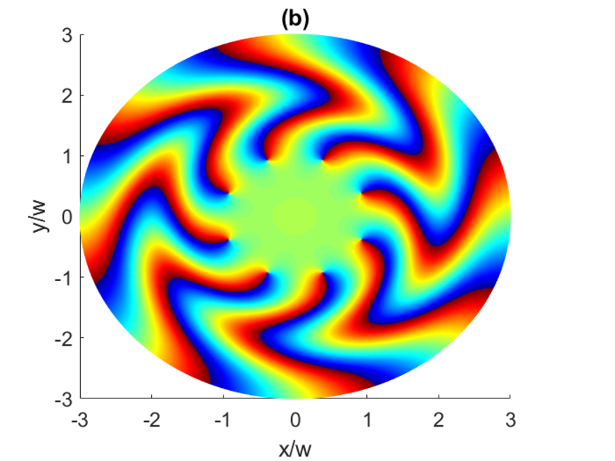
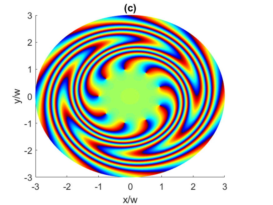
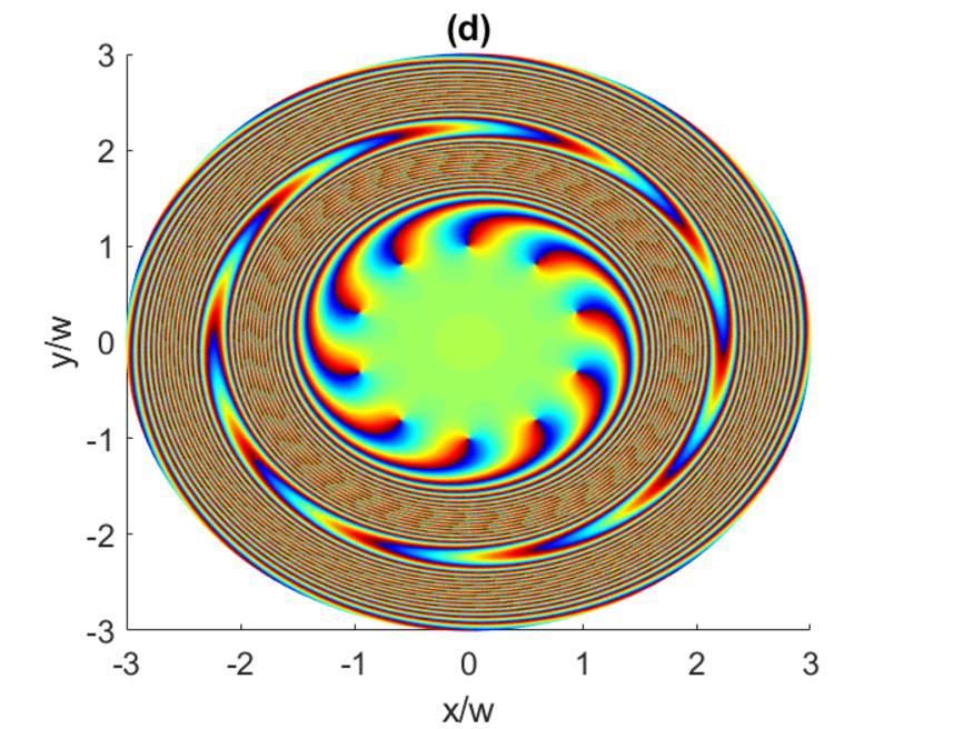
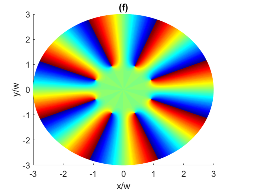
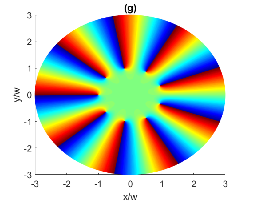
Figure 6: The helical phase patterns of the superposition beam $\psi$ featured in Eq. (25) with different vorticities $l_{1}=7$ (a, e), $l_{1}=8$ (b, f), $l_{1}=9$ (c, g) and $l_{1}=10$ (d, h). Here $\delta_{2f}=4\Gamma$ (a,b,c,d), $\delta_{2f}=0$ (e,f,g,h) and the other parameters are the same as in Fig. (2).

Comparing of Figs. 3 and 5 shows that the phase structures of the superluminal superposition beam is bent with respect to the subluminal one. Such a bending of the phase patterns becomes more significant when the topological charge $l_{1}$ increases, as one can see comparing Figs. 6 (a,b,c,d) with 6 (e,f,g,h). In fact, the exponent of the factor $e^{i\frac{\Gamma}{\delta_{1f}^{2}}\frac{\mathcal{E}_{c}^{2}(r)}{(\delta_{2f}+i\Gamma)}\frac{z}{L_{\Gamma}}}$ in Eq. (25) contains the term $\mathcal{E}_{c}^{2}(r)$ which is not uniform in the $(x,y)$ plane resulting to bending of the phase patterns when $\delta_{2f}$ is nonzero.

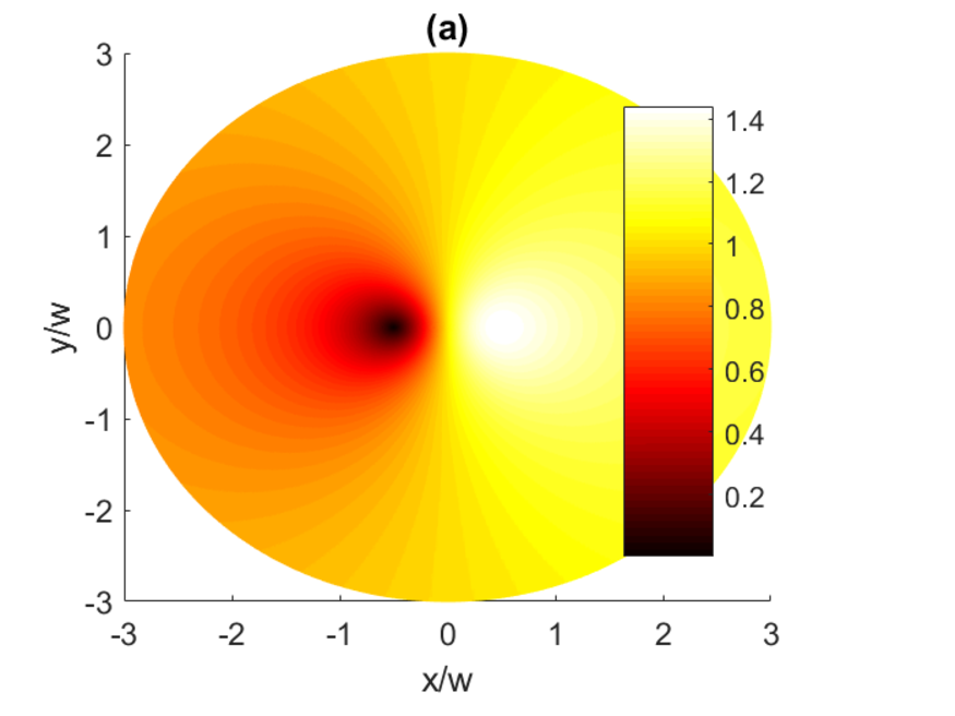
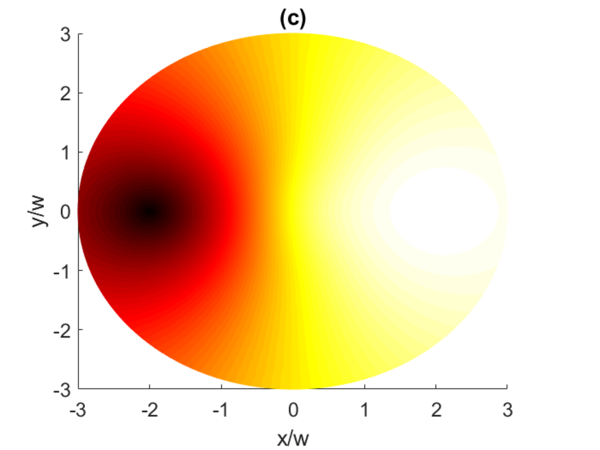
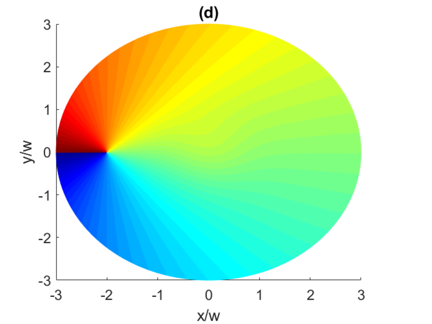
Figure 7: Intensity distributions (a, c) in arbitrary units as well as the corresponding helical phase patterns (b, d) of the superposition beam $\psi$ featured in Eq. (25). Here $|\Omega_{c_{1}}|=\Gamma$, $|\Omega_{c_{2}}|=0.5\Gamma$ (a, b) and $|\Omega_{c_{1}}|=0.5\Gamma$, $|\Omega_{c_{2}}|=\Gamma$ (c, d), $l_{1}=1$ and the other parameters are the same as in Fig. (2).

Figure 7 illustrates the effect of the strength of pump beams $|\Omega_{c_{1}}|$ and $|\Omega_{c_{2}}|$ on intensity distributions and the corresponding helical phase patterns. We plot only the case of the superluminality ($\delta_{2f}=4\Gamma$), as the results are very similar to the subluminal case. It is apparent from Fig. 7 (a, b) that the peripheral vortex shifts toward the center of the beam when $|\Omega_{c_{1}}|>|\Omega_{c_{2}}|$ while it moves away from the core when $|\Omega_{c_{1}}|<|\Omega_{c_{2}}|$ (see Fig. 7 (c, d)). As can be seen from Eq. (29), when $|\Omega_{c_{1}}|>|\Omega_{c_{2}}|$ ( $|\Omega_{c_{1}}|<|\Omega_{c_{2}}|$), the radius $r_{p}$ reduces (increases) and the position of the peripheral vortex moves radially in (out).

II.1 Exchange of optical vortices

We will now assume that only one probe field $\mathcal{P}_{1}$ is initially incident on the atomic cloud $z=0$ ($\mathcal{P}_{1}(0)=\mathcal{P}$). The amplitude of the second probe field is zero at the beginning ($\mathcal{P}_{2}(0)=0$). In this case, Eqs. (19) and (20) reduce to

$$\psi(0) =\frac{1}{\mathcal{E}_{c}(r)}\left(\mathcal{E}_{c_{1}}^{*}(r)e^{-il_{1}\varphi}\mathcal{P}\right),$$ (30)

$$\xi(0) =\frac{1}{\mathcal{E}_{c}(r)}\left(\mathcal{E}_{c_{2}}(r)e^{il_{2}\varphi}\mathcal{P}\right).$$ (31)

The electric fields of the probe beams inside the atomic cloud can be obtained from the fields $\psi$ and $\xi$ as

$$\mathcal{P}_{1}(z) =\frac{1}{\mathcal{E}_{c}(r)}\left(\mathcal{E}_{c_{1}}(r)e^{il_{1}\varphi}\psi(z)+\mathcal{E}_{c_{2}}^{*}(r)e^{-il_{2}\varphi}\xi(z)\right)=\left(1+\frac{\mathcal{E}_{c_{1}}^{2}(r)}{\mathcal{E}_{c}^{2}(r)}(e^{i\kappa z}-1)\right)\mathcal{P},$$ (32)

$$\mathcal{P}_{2}(z) =\frac{1}{\mathcal{E}_{c}(r)}\left(\mathcal{E}_{c_{2}}(r)e^{il_{2}\varphi}\psi(z)-\mathcal{E}_{c_{1}}^{*}(r)e^{-il_{1}\varphi}\xi(z)\right)=\frac{\mathcal{E}_{c_{2}}(r)\mathcal{E}_{c_{1}}^{*}(r)}{\mathcal{E}_{c}^{2}(r)}e^{i(l_{2}-l_{1})}(e^{i\kappa z}-1)\mathcal{P}.$$ (33)

where $\kappa$ is given by Eq. (24). The intensity distributions and the corresponding helical phase pattern of the generated second probe vortex beam are shown in Fig. 8 for $\delta_{2f}=4\Gamma$ and different topological charge numbers. A doughnut intensity profile is observed with a dark hollow in the center. The phase jumps from $0$ to $n\pi$ around the singularity point. As Eq. (33) shows, the generated field contains a phase factor of $e^{i(l_{2}-l_{1})}$. If the first pump field is a vortex but the second one is a non-vortex beam, the generated probe field acquires a vortex of charge $-l_{1}$. On the other hand, if only the second pump beam is a vortex with the charge $l_{2}$, the generated probe beam has a vorticity $l_{2}$.

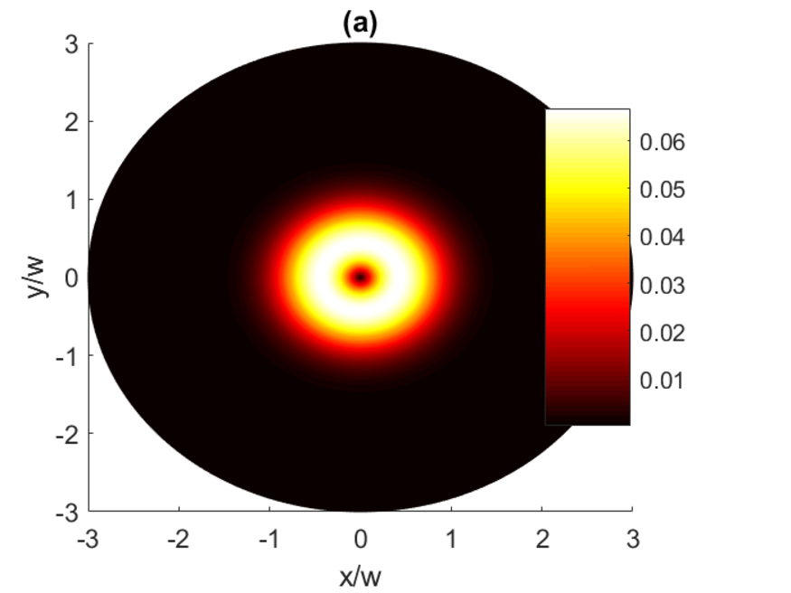
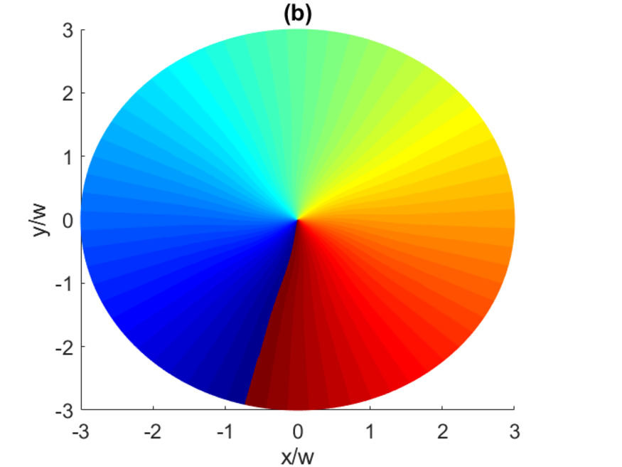
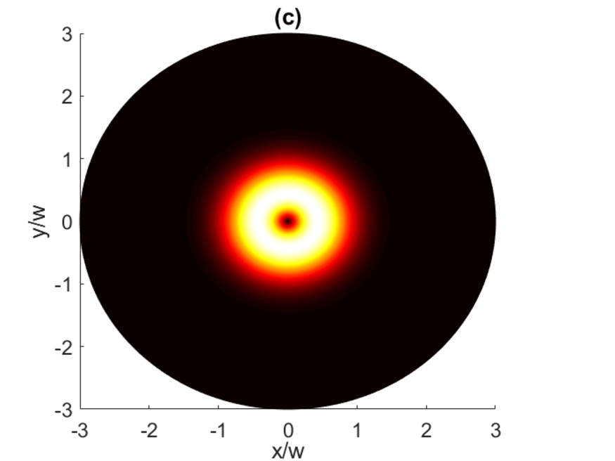
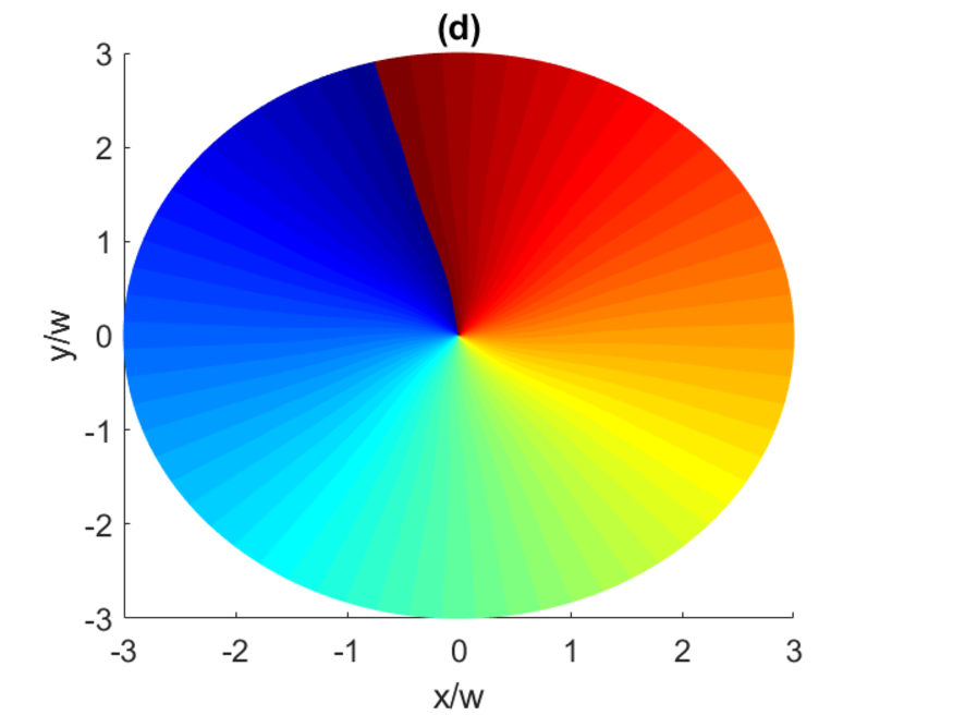
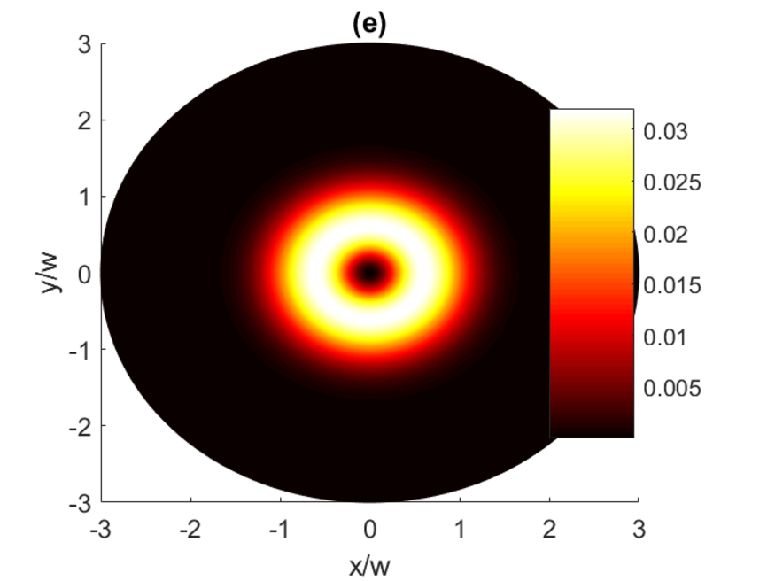
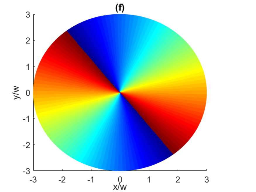
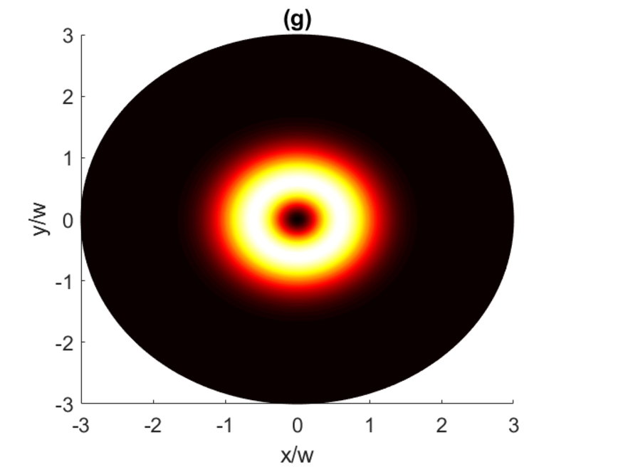
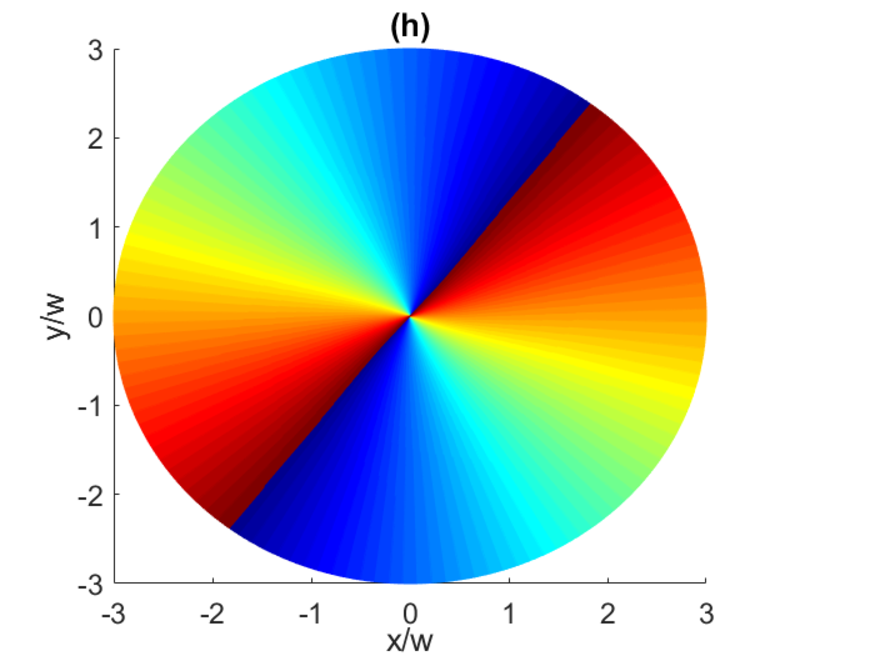
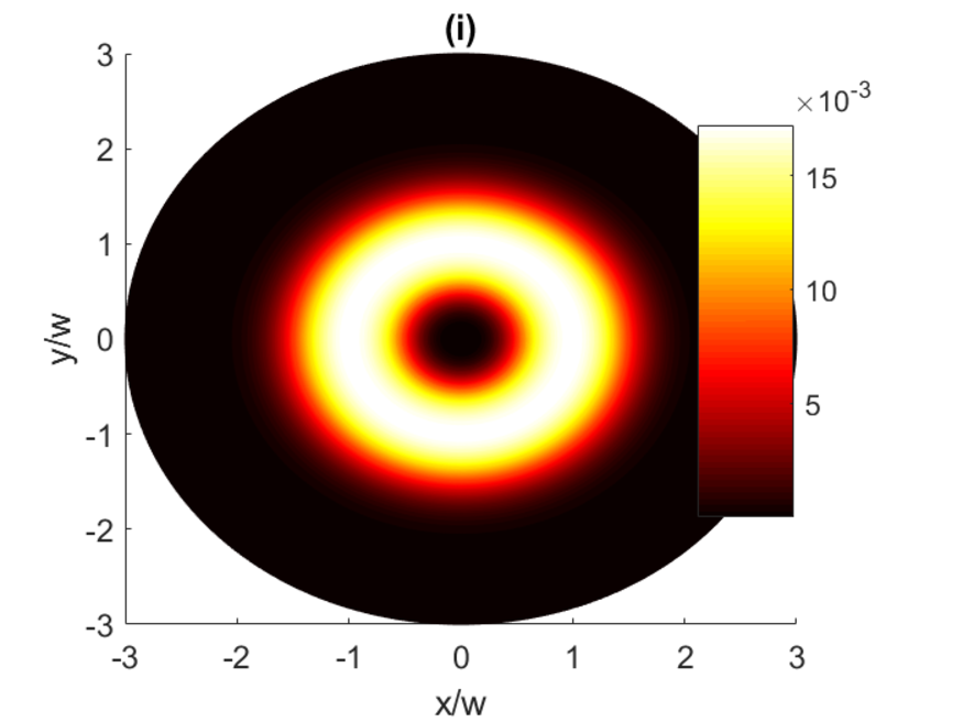
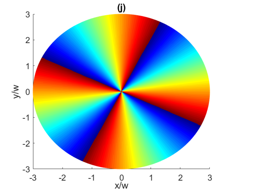
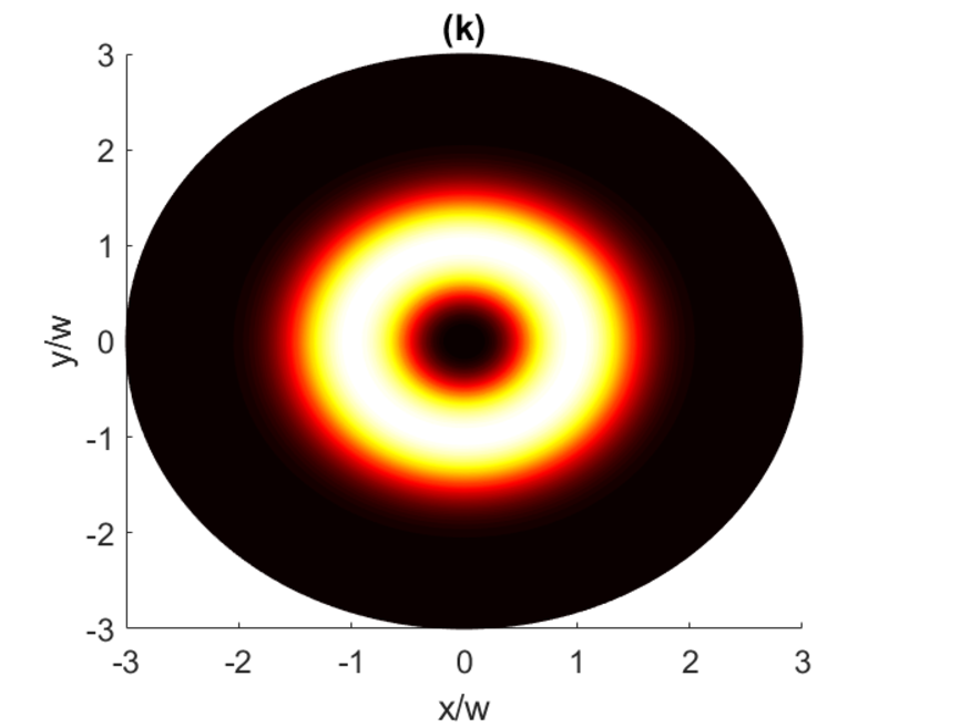
Figure 8: Intensity distributions (a, c, e, g,i,k) in arbitrary units as well as the corresponding helical phase patterns (b, d, f, h,j,l) of the generated second probe vortex beam $\mathcal{P}_{2}$ featured in Eq. (33) when $l_{1}=1$, $l_{2}=0$ (a, b), $l_{1}=0$, $l_{2}=1$ (c, d), $l_{1}=2$, $l_{2}=0$ (e, f), $l_{1}=0$, $l_{2}=1$ (g, h) and $l_{1}=4$, $l_{2}=0$ (i, j), $l_{1}=0$, $l_{2}=4$ (k, l). Here $\delta_{2f}=4\Gamma$ and the other parameters are the same as Fig. (2).

III The double Raman doublet scheme

In this section we present a more favorable scenario for the generation of off-axis vortices. We consider a situation where four strong pump beams act on the atomic ensemble (Fig. (9)). This situation corresponds to a Raman doublet for each of the probe beams.

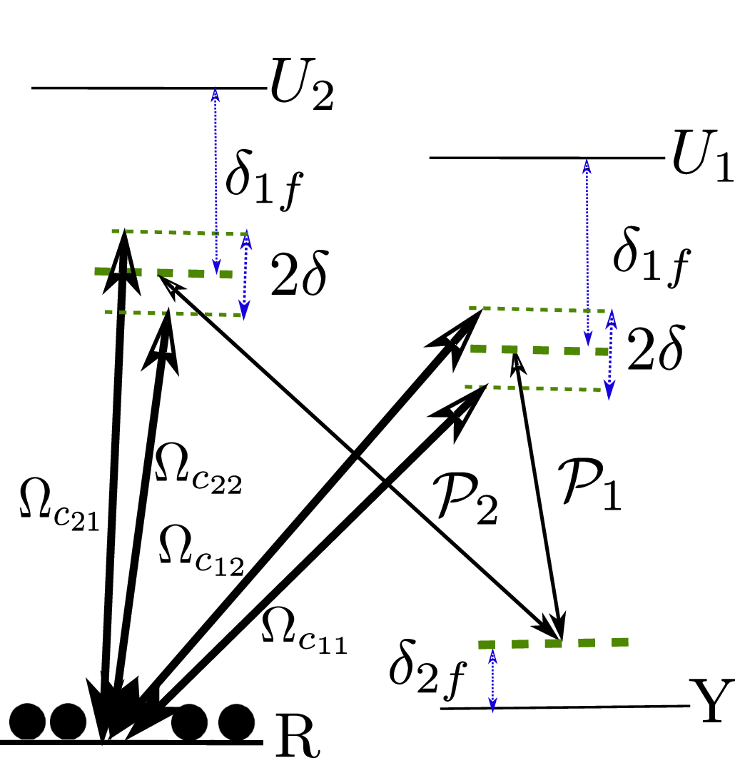
Figure 9: Schematic diagram of the double-Raman doublet scheme.

We assume four-photon resonances $\omega_{c_{11}}-\omega_{p_{1}}=\omega_{c_{21}}-\omega_{p_{2}}$, $\omega_{c_{12}}-\omega_{p_{1}}=\omega_{c_{22}}-\omega_{p_{2}}$, where $\omega_{c_{11}},$$\omega_{c_{12}}$, $\omega_{c_{21}}$ and $\omega_{c_{22}}$ are frequencies of the pump beams. To describe the propagation of the probe beams in the medium, we separate the atomic amplitudes into two parts oscillating with different frequencies: $\textbf{$\Psi_{Y}$}=\textbf{$\Psi_{Y_{1}}+\textbf{$\Psi_{Y_{2}}$}$}$, $\textbf{$\Psi_{U_{1}}$}=\textbf{$\Psi_{U_{11}}+\textbf{$\Psi_{U_{12}}$}$}$ and $\textbf{$\Psi_{U_{2}}$}=\textbf{$\Psi_{U_{21}}+\textbf{$\Psi_{U_{22}}$}$}$. Recalling the slowly changing amplitudes and neglecting the terms oscillating with a large frequency $2\delta=\omega_{c_{12}}-\omega_{c_{11}}=\omega_{c_{22}}-\omega_{c_{21}}$, the equations for the matter fields read

$$c\partial_{z}\mathcal{P}_{1}= i\alpha\Phi_{Y_{1}}^{*}\frac{\mathcal{E}_{c_{11}}(r)}{\delta_{1f}}e^{il_{11}\varphi}\Phi_{R}+i\alpha\Phi_{Y_{2}}^{*}\frac{\mathcal{E}_{c_{12}}(r)}{\delta_{1f}}e^{il_{12}\varphi}\Phi_{R},$$ (34)

$$c\partial_{z}\mathcal{P}_{2}= i\alpha\Phi_{Y_{1}}^{*}\frac{\mathcal{E}_{c_{21}}(r)}{\delta_{1f}}e^{il_{21}\varphi}\Phi_{R}+i\alpha\Phi_{Y_{2}}^{*}\frac{\mathcal{E}_{c_{22}}(r)}{\delta_{1f}}e^{il_{22}\varphi}\Phi_{R},$$ (35)

$$\Phi_{Y_{1}}= \frac{\alpha\Phi_{R}}{(\delta_{2f}+\delta-i\Gamma)\delta_{1f}}\left(\mathcal{E}_{c_{11}}(r)e^{il_{11}\varphi}\mathcal{P}_{1}^{*}+\mathcal{E}_{c_{21}}(r)e^{il_{21}\varphi}\mathcal{P}_{2}^{*}\right),$$ (36)

$$\Phi_{Y_{2}}= \frac{\alpha\Phi_{R}}{(\delta_{2f}-\delta-i\Gamma)\delta_{1f}}\left(\mathcal{E}_{c_{12}}(r)e^{il_{12}\varphi}\mathcal{P}_{1}^{*}+\mathcal{E}_{c_{22}}(r)e^{il_{22}\varphi}\mathcal{P}_{2}^{*}\right),$$ (37)

where $\delta_{1f}=\omega_{U_{1}}-\omega_{R}-\frac{1}{2}(\omega_{c_{11}}+\omega_{c_{12}})=\omega_{U_{2}}-\omega_{R}-\frac{1}{2}(\omega_{c_{21}}+\omega_{c_{22}})$ is an average one-photon detuning and $\delta_{2f}=\omega_{p_{1}}+\omega_{Y}-\omega_{R}-\frac{1}{2}(\omega_{c_{11}}+\omega_{c_{12}})=\omega_{p_{2}}+\omega_{Y}-\omega_{R}-\frac{1}{2}(\omega_{c_{21}}+\omega_{c_{22}})$ denotes an average two-photon detuning. Equations (34)-(37) give the following equations for the propagation of the probe fields

$$\partial_{z}P_{1}-i\beta\left(\frac{|\mathcal{E}_{c_{11}}(r)|^{2}\mathcal{P}_{1}+\mathcal{E}_{c_{11}}(r)\mathcal{E}_{c_{21}}^{*}(r)e^{i(l_{11}-l_{21})\varphi}\mathcal{P}_{2}}{\delta_{2f}+\delta+i\Gamma}+\frac{|\mathcal{E}_{c_{12}}(r)|^{2}\mathcal{P}_{1}+\mathcal{E}_{c_{12}}(r)\mathcal{E}_{c_{22}}^{*}(r)e^{i(l_{12}-l_{22})\varphi}\mathcal{P}_{2}}{\delta_{2f}-\delta+i\Gamma}\right) =0,$$ (38)

$$\partial_{z}P_{2}-i\beta\left(\frac{\mathcal{E}_{c_{21}}(r)\mathcal{E}_{c_{11}}^{*}(r)e^{i(l_{21}-l_{11})\varphi}\mathcal{P}_{1}+|\mathcal{E}_{c_{21}}(r)|^{2}\mathcal{P}_{2}}{\delta_{2f}+\delta+i\Gamma}+\frac{\mathcal{E}_{c_{22}}(r)\mathcal{E}_{c_{12}}^{*}(r)e^{i(l_{22}-l_{12})\varphi}\mathcal{P}_{1}+|\mathcal{E}_{c_{22}}(r)|^{2}\mathcal{P}_{2}}{\delta_{2f}-\delta+i\Gamma}\right) =0.$$ (39)

We consider a particular situation in which

$$\frac{\mathcal{E}_{c_{12}}(r)}{\mathcal{E}_{c_{11}}(r)}e^{i(l_{12}-l_{11})\varphi}=\frac{\mathcal{E}_{c_{22}}(r)}{\mathcal{E}_{c_{21}}(r)}e^{i(l_{22}-l_{21})\varphi}.$$ (40)

Defining the generalized quantities

$$\mathcal{E}_{c_{1}}(r) =\sqrt{|\mathcal{E}_{c_{11}}(r)|^{2}+|\mathcal{E}_{c_{21}}(r)|^{2}},$$ (41)

$$\mathcal{E}_{c_{2}}(r) =\sqrt{|\mathcal{E}_{c_{12}}(r)|^{2}+|\mathcal{E}_{c_{22}}(r)|^{2}},$$ (42)

and introducing new fields representing superpositions of the original probe fields

$$\psi=\frac{1}{\mathcal{E}_{c_{1}}(r)}\left(\mathcal{E}_{c_{11}}^{*}(r)e^{-il_{11}\varphi}\mathcal{P}_{1}+\mathcal{E}_{c_{21}}^{*}(r)e^{-il_{21}\varphi}\mathcal{P}_{2}\right),$$ (43)

$$\xi=\frac{1}{\mathcal{E}_{c_{1}}(r)}\left(\mathcal{E}_{c_{21}}(r)e^{il_{21}\varphi}\mathcal{P}_{1}-\mathcal{E}_{c_{11}}(r)e^{il_{11}\varphi}\mathcal{P}_{2}\right),$$ (44)

reduce Eqs. (38) and (39) to Eqs. (22) and (23) with

$$\kappa=\beta\left(\frac{\mathcal{E}_{c_{1}}^{2}(r)}{(\delta_{2f}+\delta+i\Gamma)}+\frac{\mathcal{E}_{c_{2}}^{2}(r)}{(\delta_{2f}-\delta+i\Gamma)}\right).$$ (45)

Again, the field $\xi$ does not interact and propagates as in free space, while the new field $\psi$ interacts with the atoms. Assuming

$$\mathcal{E}_{c_{1}}(r)=\mathcal{E}_{c_{2}}(r)=\mathcal{E}_{c}(r),$$ (46)

and $\delta_{2f}=0$, one finds

$$\nu_{g}=\frac{c}{1+\frac{2\alpha^{2}n\mathcal{E}_{c}^{2}(r)}{\delta_{1f}^{2}}\frac{\Gamma^{2}-\delta^{2}}{(\delta^{2}+\Gamma^{2})^{2}}}.$$ (47)

Thus for $\delta>\Gamma$ ($\delta<\Gamma$) the group velocity is larger (smaller) than $c$ providing superluminal (superluminal) propagation. In addition, according to the Eq. (45) , the generated fast light experiences again amplification. We see that, in contrast to the double-Raman scheme, we have sup- or superluminal propagation even for zero two-photon detuning $\delta_{2f}=0$. In order to have off-axis optical vortices satisfying Eqs. (40), (41), (42), (46) and to avoid zero denominator at the core in $\psi(z)=\psi(0)e^{i\kappa z}$, we can consider $l_{11}=-l_{22}=l\neq 0$ (i.e. $\Omega_{c_{11}}$ and $\Omega_{c_{22}}$ are vortices) but $l_{21}=l_{12}=0$ (i.e. $\Omega_{c_{11}}$ and $\Omega_{c_{22}}$ are non-vortex Gaussian beams).

Let us assume that only one probe field $\mathcal{P}_{1}$ is incident on the atomic cloud ($\mathcal{P}_{1}(0)=\mathcal{P}$). The amplitude of the second probe field at the beginning of the atomic cloud $z=0$ is zero ($\mathcal{P}_{2}(0)=0$). In this case, Eqs. (43) and (44) reduce to

$$\psi(0) =\frac{\mathcal{E}_{c_{11}}^{*}(r)e^{-il\varphi}}{\mathcal{E}_{c_{1}}(r)}\mathcal{P},$$ (48)

$$\xi(0) =\frac{\mathcal{E}_{c_{21}}(r)}{\mathcal{E}_{c_{1}}(r)}\mathcal{P}.$$ (49)

The electric fields of the probe beams inside the atomic cloud can be obtained from the fields $\psi$ and $\xi$ as

$$\mathcal{P}_{1}(z) =\left(1+\frac{\mathcal{E}_{c_{11}}^{2}(r)}{\mathcal{E}_{c}^{2}(r)}(e^{i\kappa z}-1)\right)\mathcal{P},$$ (50)

$$\mathcal{P}_{2}(z) =\frac{\mathcal{E}_{c_{21}}(r)\mathcal{E}_{c_{11}}^{*}(r)}{\mathcal{E}_{c}^{2}(r)}e^{-il\varphi}(e^{i\kappa z}-1)\mathcal{P},$$ (51)

with $\kappa$ featured in Eq. (45). Exchange of optical vortices with opposite vorticity is now possible between the pump field $\Omega_{c_{11}}$ and the generated probe field $\mathcal{P}_{2}$ even for zero two-photon detuning $\delta_{2f}=0$.

IV Summary

We have investigated the formation of off-axis vortices with shifted axes in a double-Raman gain medium interacting with two weak probe fields as well as two stronger pump lasers which can contain an optical vortex. In such a medium only a particular superposition of the probe fields is coupled with the atoms, while an orthogonal combination of the probe fields does not interact with the atoms and propagates as in the free space. Assuming that one of the pump fields is a vortex, depending on the two-photon detuning, the superposition off-axis vortex beam can propagate either with the slow or the fast group velocity. One can control the position of the peripheral vortices by the vorticity and intensity of the pump fields. The model for creation of the off-center fast and slow light vortices can also be generalized to a more complicated double Raman doublet with four pump fields. A possible experimental realization of the proposed scheme for off-axis optical vortices can be implemented for an atomic cesium vapor cell at the room temperature. All cesium atoms are to be prepared in the ground-state hyperfine magnetic sublevel $6S_{1/2},|F=4,m=-4\rangle$ serving as the level $R$ in our scheme. The magnetic sublevel $6S_{1/2},|F=4,m=-2\rangle$ corresponds to the level $Y$. Also, the levels $5P_{3/2},|F=4,m=-3\rangle$ and $6P_{1/2},|F=4,m=-3\rangle$ are excited levels $U_{1}$and $U_{2}$, respectively Kudriašov et al. (2014).

References

- Harris (1997) S. E. Harris, Physics Today 50, 36 (1997).
- Fleischhauer et al. (2005) M. Fleischhauer, A. Imamoglu, and J. P. Marangos, Rev. Mod. Phys. 77, 633 (2005), URL https://link.aps.org/doi/10.1103/RevModPhys.77.633.
- Paspalakis et al. (2002) E. Paspalakis, N. J. Kylstra, and P. L. Knight, Phys. Rev. A 65, 053808 (2002), URL https://link.aps.org/doi/10.1103/PhysRevA.65.053808.
- Paspalakis and Kis (2002a) E. Paspalakis and Z. Kis, Phys. Rev. A 66, 025802 (2002a), URL https://link.aps.org/doi/10.1103/PhysRevA.66.025802.
- Paspalakis and Kis (2002b) E. Paspalakis and Z. Kis, Phys. Rev. A 66, 025802 (2002b), URL https://link.aps.org/doi/10.1103/PhysRevA.66.025802.
- Ruseckas et al. (2007) J. Ruseckas, G. Juzeliūnas, P. Öhberg, and S. M. Barnett, Phys. Rev. A 76, 053822 (2007), URL https://link.aps.org/doi/10.1103/PhysRevA.76.053822.
- Grobe et al. (1994) R. Grobe, F. T. Hioe, and J. H. Eberly, Phys. Rev. Lett. 73, 3183 (1994), URL https://link.aps.org/doi/10.1103/PhysRevLett.73.3183.
- Fleischhauer and Manka (1996) M. Fleischhauer and A. S. Manka, Phys. Rev. A 54, 794 (1996), URL https://link.aps.org/doi/10.1103/PhysRevA.54.794.
- Wang et al. (2001) H. Wang, D. Goorskey, and M. Xiao, Phys. Rev. Lett. 87, 073601 (2001), URL https://link.aps.org/doi/10.1103/PhysRevLett.87.073601.
- Harris (1994) S. E. Harris, Phys. Rev. Lett. 72, 52 (1994), URL https://link.aps.org/doi/10.1103/PhysRevLett.72.52.
- Cerboneschi and Arimondo (1995) E. Cerboneschi and E. Arimondo, Phys. Rev. A 52, R1823 (1995), URL https://link.aps.org/doi/10.1103/PhysRevA.52.R1823.
- Harris et al. (1990) S. E. Harris, J. E. Field, and A. Imamoğlu, Phys. Rev. Lett. 64, 1107 (1990), URL https://link.aps.org/doi/10.1103/PhysRevLett.64.1107.
- Deng et al. (1998) L. Deng, M. G. Payne, and W. R. Garrett, Phys. Rev. A 58, 707 (1998), URL https://link.aps.org/doi/10.1103/PhysRevA.58.707.
- Kang and Zhu (2003) H. Kang and Y. Zhu, Phys. Rev. Lett. 91, 093601 (2003), URL https://link.aps.org/doi/10.1103/PhysRevLett.91.093601.
- Hamedi and Juzeliūnas (2015) H. R. Hamedi and G. Juzeliūnas, Phys. Rev. A 91, 053823 (2015), URL https://link.aps.org/doi/10.1103/PhysRevA.91.053823.
- Wu and Deng (2004a) Y. Wu and L. Deng, Phys. Rev. Lett. 93, 143904 (2004a), URL https://link.aps.org/doi/10.1103/PhysRevLett.93.143904.
- Wu and Deng (2004b) Y. Wu and L. Deng, Opt. Lett. 29, 2064 (2004b).
- Hau et al. (1999) L. V. Hau, S. E. Harris, Z. Dutton, and C. H. Behroozi, Nature 397, 594 (1999).
- Lukin (2003) M. D. Lukin, Rev. Mod. Phys. 75, 457 (2003), URL https://link.aps.org/doi/10.1103/RevModPhys.75.457.
- Juzeliūnas and Öhberg (2004) G. Juzeliūnas and P. Öhberg, Phys. Rev. Lett. 93, 033602 (2004), URL https://link.aps.org/doi/10.1103/PhysRevLett.93.033602.
- Ruseckas et al. (2011a) J. Ruseckas, V. Kudriašov, G. Juzeliūnas, R. G. Unanyan, J. Otterbach, and M. Fleischhauer, Phys. Rev. A 83, 063811 (2011a).
- Bao et al. (2011) Q.-Q. Bao, X.-H. Zhang, J.-Y. Gao, Y. Zhang, C.-L. Cui, and J.-H. Wu, Phys. Rev. A 84, 063812 (2011).
- Ruseckas et al. (2013) J. Ruseckas, V. Kudriašov, I. A. Yu, and G. Juzeliūnas, Phys. Rev. A 87, 053840 (2013), URL https://link.aps.org/doi/10.1103/PhysRevA.87.053840.
- Lee et al. (2014) M.-J. Lee, J. Ruseckas, C.-Y. Lee, V. Kudriašov, K.-F. Chang, H.-W. Cho, G. Juzeliūnas, and I. A. Yu, Nature Communications 5, 5542 (2014).
- Phillips et al. (2001) D. F. Phillips, A. Fleischhauer, A. Mair, R. L. Walsworth, and M. D. Lukin, Phys. Rev. Lett. 86, 783 (2001), URL https://link.aps.org/doi/10.1103/PhysRevLett.86.783.
- Liu et al. (2001) C. Liu, Z. Dutton, C. H. Behroozi, and L. V. Hau, Nature 409 (2001).
- Lukin and Imamoglu (2001) M. D. Lukin and A. Imamoglu, Nature 413 (2001).
- Juzeliūnas and Carmichael (2002) G. Juzeliūnas and H. J. Carmichael, Phys. Rev. A 65, 021601(R) (2002).
- Ma et al. (2017) L. Ma, O. Slattery, and X. Tang, J. Opt. 19, 043001 (2017).
- Hsiao et al. (2018) Y.-F. Hsiao, P.-J. Tsai, H.-S. Chen, S.-X. Lin, C.-C. Hung, C.-H. Lee, Y.-H. Chen, Y.-F. Chen, I. A. Yu, and Y.-C. Chen, Phys. Rev. Lett. 120, 183602 (2018), URL https://link.aps.org/doi/10.1103/PhysRevLett.120.183602.
- Jiang et al. (2007) K. J. Jiang, L. Deng, and M. G. Payne, Phys. Rev. A 76, 033819 (2007), URL https://link.aps.org/doi/10.1103/PhysRevA.76.033819.
- M.Mahmoudi et al. (2006) M.Mahmoudi, M.Sahrai, and H.Tajalli, Phys. Lett. A 357, 66 (2006).
- qi Kuang et al. (2009) S. qi Kuang, R. gang Wan, J. Kou, Y. Jiang, , and J. yue Gao, J. Opt. Soc. Am. B 26, 2256 (2009).
- Akulshin and McLean (2010) A. M. Akulshin and R. J. McLean, J. Opt. 12, 104001 (2010).
- Chu and Wong (1982) S. Chu and S. Wong, Phys. Rev. Lett. 48, 738 (1982), URL https://link.aps.org/doi/10.1103/PhysRevLett.48.738.
- Steinberg et al. (1993) A. M. Steinberg, P. G. Kwiat, and R. Y. Chiao, Phys. Rev. Lett. 71, 708 (1993), URL https://link.aps.org/doi/10.1103/PhysRevLett.71.708.
- Chiao (1993) R. Y. Chiao, Phys. Rev. A 48, R34 (1993), URL https://link.aps.org/doi/10.1103/PhysRevA.48.R34.
- Dogariu et al. (2001) A. Dogariu, A. Kuzmich, and L. J. Wang, Phys. Rev. A 63, 053806 (2001), URL https://link.aps.org/doi/10.1103/PhysRevA.63.053806.
- Glasser et al. (2012) R. T. Glasser, U. Vogl, and P. D. Lett, Phys. Rev. Lett. 108, 173902 (2012), URL https://link.aps.org/doi/10.1103/PhysRevLett.108.173902.
- Bianucci et al. (2008) P. Bianucci, C. R. Fietz, J. W. Robertson, G. Shvets, and C.-K. Shih, Phys. Rev. A 77, 053816 (2008), URL https://link.aps.org/doi/10.1103/PhysRevA.77.053816.
- Kudriašov et al. (2014) V. Kudriašov, J. Ruseckas, A. Mekys, A. Ekers, N. Bezuglov, and G. Juzeliūnas, Phys. Rev. A 90, 033827 (2014), URL https://link.aps.org/doi/10.1103/PhysRevA.90.033827.
- Allen et al. (1999) L. Allen, M. J. Padgett, and M. Babiker, Progress in Optics 39, 291 (1999).
- Padgett et al. (2004) M. Padgett, J. Courtial, and L. Allen, Physics Today 57, 35 (2004).
- Babiker et al. (2018) M. Babiker, D. L. Andrews, and V. E. Lembessis, Journal of Optics 21, 013001 (2018), URL https://doi.org/10.1088%2F2040-8986%2Faaed14.
- Babiker et al. (1994) M. Babiker, W. L. Power, and L. Allen, Phys. Rev. Lett. 73, 1239 (1994), URL https://link.aps.org/doi/10.1103/PhysRevLett.73.1239.
- Molina-Terriza et al. (2001) G. Molina-Terriza, J. P. Torres, and L. Torner, Phys. Rev. Lett. 88, 013601 (2001), URL https://link.aps.org/doi/10.1103/PhysRevLett.88.013601.
- Pugatch et al. (2007) R. Pugatch, M. Shuker, O. Firstenberg, A. Ron, and N. Davidson, Phys. Rev. Lett. 98, 203601 (2007), URL https://link.aps.org/doi/10.1103/PhysRevLett.98.203601.
- Dutton and Ruostekoski (2004) Z. Dutton and J. Ruostekoski, Phys. Rev. Lett. 93, 193602 (2004), URL https://link.aps.org/doi/10.1103/PhysRevLett.93.193602.
- Bishop et al. (2004) A. I. Bishop, T. A. Nieminen, N. R. Heckenberg, and H. Rubinsztein-Dunlop, Phys. Rev. Lett. 92, 198104 (2004), URL https://link.aps.org/doi/10.1103/PhysRevLett.92.198104.
- Chen et al. (2008) Q.-F. Chen, B.-S. Shi, Y.-S. Zhang, and G.-C. Guo, Phys. Rev. A 78, 053810 (2008), URL https://link.aps.org/doi/10.1103/PhysRevA.78.053810.
- Lembessis and Babiker (2010) V. E. Lembessis and M. Babiker, Phys. Rev. A 82, 051402 (2010), URL https://link.aps.org/doi/10.1103/PhysRevA.82.051402.
- Ruseckas et al. (2011b) J. Ruseckas, A. Mekys, and G. Juzeliūnas, J. Opt. 13, 064013 (2011b).
- Ding et al. (2012) D.-S. Ding, Z.-Y. Zhou, B.-S. Shi, X.-B. Zou, and G.-C. Guo, Opt. Lett. 37, 3270 (2012).
- Walker et al. (2012) G. Walker, A. S. Arnold, and S. Franke-Arnold, Phys. Rev. Lett. 108, 243601 (2012), URL https://link.aps.org/doi/10.1103/PhysRevLett.108.243601.
- Lembessis et al. (2014) V. E. Lembessis, D. Ellinas, M. Babiker, and O. Al-Dossary, Phys. Rev. A 89, 053616 (2014), URL https://link.aps.org/doi/10.1103/PhysRevA.89.053616.
- Radwell et al. (2015) N. Radwell, T. W. Clark, B. Piccirillo, S. M. Barnett, and S. Franke-Arnold, Phys. Rev. Lett. 114, 123603 (2015), URL https://link.aps.org/doi/10.1103/PhysRevLett.114.123603.
- Sharma and Dey (2017) S. Sharma and T. N. Dey, Phys. Rev. A 96, 033811 (2017), URL https://link.aps.org/doi/10.1103/PhysRevA.96.033811.
- Hamedi et al. (2018a) H. R. Hamedi, V. Kudriašov, J. Ruseckas, and G. Juzeliūnas, Optics Express 26, 28249 (2018a).
- Hamedi et al. (2018b) H. R. Hamedi, J. Ruseckas, and G. Juzeliūnas, Phys. Rev. A 98, 013840 (2018b), URL https://link.aps.org/doi/10.1103/PhysRevA.98.013840.
- Hamedi et al. (2019a) H. R. Hamedi, J. Ruseckas, E. Paspalakis, and G. Juzeliūnas, Phys. Rev. A 99, 033812 (2019a), URL https://link.aps.org/doi/10.1103/PhysRevA.99.033812.
- Moretti et al. (2009) D. Moretti, D. Felinto, and J. W. R. Tabosa, Phys. Rev. A 79, 023825 (2009), URL https://link.aps.org/doi/10.1103/PhysRevA.79.023825.
- Cardano et al. (2015) F. Cardano, F. Massa, H. Qassim, E. Karimi, S. Slussarenko, D. Paparo, C. de Lisio, F. Sciarrino, E. Santamato, R. W. Boyd, et al., Science Advances 1, e1500087 (2015).
- Hamedi et al. (2019b) H. R. Hamedi, E. Paspalakis, G. Žlabys, G. Juzeliūnas, and J. Ruseckas, Phys. Rev. A 100, 023811 (2019b), URL https://link.aps.org/doi/10.1103/PhysRevA.100.023811.
- Hong et al. (2019) Y. Hong, Z. Wang, D. Ding, and B. Yu, Optics Express 27, 29863 (2019).
- Qiu et al. (2020) J. Qiu, Z. Wang, D. Ding, W. Li, , and B. Yu, Optics Express 28, 2975 (2020).
- Maleev and Swartzlander (2003) I. D. Maleev and G. A. Swartzlander, J. Opt. Soc. Am. B 20, 1169 (2003).
- Galvez et al. (2006) E. J. Galvez, N. Smiley, and N. Fernandes, Proc. SPIE 6131, 613105 (2006).
- Baumann et al. (2009) S. M. Baumann, D. M. Kalb, L. H. MacMillan, and E. J. Galvez, Optics Express 17, 9818 (2009).
- Mair et al. (2001) A. Mair, A. Vaziri, G. Weihs, and A. Zeilinger, Nature 412 (2001).
- Basistiy et al. (2003) I. V. Basistiy, V. V. Slyusar, M. S. Soskin, M. V. Vasnetsov, and A. Y. Bekshaev, Opt. Lett. 28, 1185 (2003).
- Lee et al. (2005) W. M. Lee, B. P. S. Ahluwalia, X.-C. Yuan, W. C. Cheong, and K. Dholakia, J. Opt. A: Pure Appl. Opt. 7, 1 (2005).
- Wang (2017) X. Z. H. Wang, Opt. Commun. 403, 358 (2017).