An explicit univariate and radical parametrization of the septic proper Zolotarev polynomials in power form

Abstract

The problem of determining an explicit one-parameter power form representation of the proper $n$-th degree Zolotarev polynomials on $[-1,1]$ can be traced back to P. L. Chebyshev, see [41]. It turned out to be complicated, even for small values of $n$. Such a representation was known to A. A. Markov (1889) [18] for $n=2$ and $n=3$, see also [5]. But already for $n=4$ it seems that nobody really believed that an explicit form can be found. As a matter of fact it was, by V. A. Markov in 1892 [20], as A. Shadrin put it in 2004 [34], see also [27], [28]. The next higher degrees, $n=5$ and $n=6$, were resolved only recently, by G. Grasegger and N. Th. Vo (2017) [10] respectively by the present authors (2019) [31]. In this paper we settle the case $n=7$ using symbolic computation. The parametrization for the degrees $n\in\{2,3,4\}$ is a rational one, whereas for $n\in\{5,6,7\}$ it is a radical one. However, the case $n=7$ among the radical parametrizations requires special attention, since it is not a simple radical one.

1 Introduction and historical remarks

With $||.||_{\infty}$ denoting the uniform norm on $\boldsymbol{I}=[-1,1]\subset\mathbb{R}$, Chebyshev [6] found that

$$\min_{(a_{0,n},\cdots,a_{n-1,n)}\in\mathbb{R}^{n}}||\widetilde{P}_{n}||_{\infty}=2^{1-n},\hbox{ where }\widetilde{P}_{n}(x)=\sum_{k=0}^{n-1}a_{k,n}\,x^{k}+x^{n}.$$ (1)

The least possible value $2^{1-n}$ is attained if $\widetilde{P}_{n}(x)={\widetilde{P}}^{*}_{n}(x)=2^{1-n}T_{n}(x)=\sum_{k=0}^{n-1}a_{k,n}^{*}\,x^{k}+x^{n}$ with known optimal coefficients $a_{k,n}^{*}$. Here $T_{n}$ with $||T_{n}||_{\infty}=1$ denotes the $n$-th (normalized) Chebyshev polynomial of the first kind with respect to $\boldsymbol{I}$, see [33, p. 6, p. 67] or [21, p. 384] for details. In 1867 Chebyshev himself proposed to his student E. I. Zolotarev, see [40, p. 2], an extension of (1) by requiring that not only the first but also the second leading coefficient, $a_{n-1,n}$, is to be kept fixed. This extension was later re-named as Zolotarev’s first problem (ZFP) and amounts, for a given $n\geq 2$, to the determination of

$$\min_{(a_{0,n},\cdots,a_{n-2,n)}\in\mathbb{R}^{n-1}}||\widetilde{Z}_{n,s}||_{\infty}=L_{n}(s),\,\hbox{where}$$ (2)

$$\widetilde{Z}_{n,s}(x)=\sum_{k=0}^{n-2}a_{k,n}\,x^{k}+(-ns)x^{n-1}+x^{n},$$

and of the extremal polynomial, $\widetilde{Z}^{*}_{n,s}$, where $s\in\mathbb{R}$ is assumed. Thus $a_{n,n}=1$ and the second leading coefficient, $a_{n-1,n}=(-ns)$, although thought of as being fixed, may attain arbitrary values, so that we save the notation $s_{0}$ for a concrete prescribed number $s$. Correspondingly, we shall then write $L_{n}(s_{0})$ for a concrete minimum in (2) and $\widetilde{Z}^{*}_{n,s_{0}}$ for a concrete extremal (minimal) polynomial. It is well known that one may restrict the range of $s$ to $s>0$, and that, for $0<s\leq\tan^{2}(\frac{\pi}{2n})$, $\widetilde{Z}^{*}_{n,s}$ is given by a distorted $\widetilde{P}^{*}_{n}$, see e.g. [1, p. 16], [2, p. 57], [5], [21, p. 405] for details, and is called a monic improper Zolotarev polynomial.

For the range $s>\tan^{2}(\frac{\pi}{2n})$ however, on which we focus in this paper, the solution $\widetilde{Z}^{*}_{n,s}$ of ZFP is considered as very complicated, see e.g. [1, p. 27], [5], [21, p. 407], [23], as unwieldy [36, p. 118], or even as mysterious [37], and is called a monic proper [34], [38, p. 160] or hard-core [21, p. 407], [32] Zolotarev polynomial. The min-max-problems in (1) and (2) can be viewed as problems of best uniform approximation to $x^{n}$ respectively $(-ns)x^{n-1}+x^{n}$ by polynomials of degree $n-1$ respectively $n-2$.

Zolotarev provided $\widetilde{Z}^{*}_{n,s}$ in 1868 [40] and in a reworked form in 1877 [41], however not, as is suggested by the task (2), in an algebraic power form with explicit optimal coefficients. Rather, he presented $\widetilde{Z}^{*}_{n,s}$ in terms of elliptic integrals and functions, see also e.g. [1, p. 18], [2, p. 280], [5], [9], [15], [21, p. 407], [25] for details. A. A. Markov [19, p. 264] expressed his reservation about Zolotarev’s solution: Being based on the application of elliptic functions, Zolotarev’s solution is too complicated to be useful in practice. As it is expounded in [5, Section 3], to deduce from Zolotarev’s elliptic solution an algebraic power form solution (sometimes called synthesizing [7, p. 1066]) turns out to be unexpectedly complicated, even for the first reasonable polynomial degree $n=2$. As F. Peherstorfer put it in 2006 [26, p. 143], there was and still is a demand for a description [of proper Zolotarev polynomials] without elliptic functions. In literature there are scattered several approaches to solve ZFP algebraically and thus to avoid the use of elliptic functions, see [31, Section 1].

But when it comes down to represent the monic proper Zolotarev polynomial $\widetilde{Z}^{*}_{n,s}$, or its normalized version $Z^{*}_{n,s}=\widetilde{Z}^{*}_{n,s}/L_{n}(s)$ (with $||Z^{*}_{n,s}||_{\infty}=1$), as a polynomial of degree $n$ in power form with explicit parameterized coefficients, then such solutions are known only for $2\leq n\leq 6$, see Section 2 below. Upon using symbolic computation as implemented in Maple [17] and Mathematica [39], we are now able to provide such an explicit power form solution even for the degree $n=7$, see Section 3 below. This contributes to the solution of ZFP which is one of E. Kaltofen’s favorite open problems in symbolic computation [13, Section 2]. In the conference paper [14] it is claimed to have solved ZFP by symbolic computation even for $6\leq n\leq 12$, but actually a theoretical solution strategy is delineated, without providing a solution formula or a concrete example, and in particular without representing the extremal polynomial in a parameterized power form for a given $n$. For an algorithm-based algebraic solution formula to ZFP for $6\leq n\leq 12$ see [30].

2 Explicit analytical one-parameter power form representation of the proper Zolotarev polynomials of degree $2\leq n\leq 6$

With the goal to find a convenient parametrization for the coefficients of the extremal polynomial in (2) with a parameter $t\in I_{n}$ from some finite open parameter interval $I_{n}\subset\mathbb{R}$ $(n>2)$, and following the literature, see [10], [22, Secton 14], [27], [31], [34, Section 1.4], we now change our notation and strive to obtain the solution of ZFP in the form

$$\widetilde{Z}_{n,t}(x)=\sum_{k=0}^{n-2}a_{k,n}(t)\,x^{k}+(-ns(t))x^{n-1}+x^{n},$$ (3)

where the explicit coefficients $a_{k,n}(t)$ and $-ns(t)$ depend injectively on $t\in I_{n}$. The least deviation (on $\boldsymbol{I}$) of $\widetilde{Z}_{n,t}$ from the zero-function is $||\widetilde{Z}_{n,t}||_{\infty}=L_{n}(t)$. For a prescribed $t=t_{0}\in I_{n}$ there holds $\min_{(a_{0,n},\dots,a_{n-2,n})\in\mathbb{R}^{n-1}}||P_{n}||_{\infty}$ $=L_{n}(t_{0})$, where $P_{n}(x)=\sum_{k=0}^{n-2}a_{k,n}x^{k}+(-ns(t_{0}))x^{n-1}+x^{n}$. Thus, for a given fixed degree $n$, (3) represents an infinite family of $n$-th degree monic proper Zolotarev polynomials. For a prescribed $s=s_{0}\in(\tan^{2}\left(\frac{\pi}{2n}\right),\infty)$ one then has to solve the equation $s(t)=s_{0}$ for $t$ and to insert the unique solution $t=t_{0}\in I_{n}$ into $\widetilde{Z}_{n,t}(x)$ in order to get the desired solution $\widetilde{Z}^{*}_{n,s_{0}}(x)=\widetilde{Z}_{n,t_{0}}(x)$ in (2) for the given $s=s_{0}$.

Analogously, we will denote by

$$Z_{n,t}(x)=\sum_{k=0}^{n}b_{k,n}(t)x^{k}\hbox{ with }t\in I_{n}\hbox{ and }b_{n,n}(t)\neq 0$$ (4)

the normalized proper Zolotarev polynomials $Z_{n,t}=\widetilde{Z}_{n,t}/L_{n}(t)$ with $||Z_{n,t}||_{\infty}$$=1$. For a prescribed $s=s_{0}\in(\tan^{2}\left(\frac{\pi}{2n}\right),\infty)$ one then has to equate $b_{n-1,n}(t)/$ $b_{n,n}(t)$ with $(-ns_{0})$ and to solve for $t$, and finally to insert the unique solution $t=t_{0}\in I_{n}$ into $Z_{n,t}(x)/b_{n,n}(t)$ in order to get the desired solution $\widetilde{Z}^{*}_{n,s_{0}}(x)=Z_{n,t_{0}}(x)/b_{n,n}(t_{0})$ in (2) for the given $s=s_{0}$.

So the key question is: How to choose the parameter intervals $I_{n}$ and the parameterized coefficients $a_{k,n}(t)$ and $-ns(t)$ in (3) respectively $b_{k,n}(t)$ in (4)? Before providing an answer for $n=7$ we first allude to known solutions $Z_{n,t}$ (possibly after some rearrangement) for the polynomial degrees $2\leq n\leq 6$:

For $n=2$ and $n=3$ see [5], [10], [15, p. 246], [18], [22, p. 156], [29], [38, p. 98].

For $n=4$ see [10], [15, p. 246], [20, p. 73], [27], [28], [34], and note the remarkable comment by Shadrin [34, Section 1.4] as quoted in the Abstract of the present paper.

Still in 2014 Shadrin [35, p. 1185] was right in writing that there is no explicit expression for [normalized proper] Zolotarev polynomials of degree $n>4$. But already in 2017 Grasegger & Vo [10] provided such an explicit expression for the degree $n=5$, see also [8], [16], [29].

Only two years later the present authors provided such an explicit expression for the degree $n=6$, see [31]. It goes without saying that the complexity of the explicit expressions (3) and (4) increases dramatically when the degree $n$ grows, see also corresponding remarks in [3, p. 511], [4, p. 21], [16, p. 932]. A further complication creeps in due to the fact that the parametrization in (3) and (4) is a radical one for $n\in\{5,6,7\}$ (obtained by computer-aided symbolic computation), whereas it is a rational one for $n\in\{2,3,4\}$ (obtained by pencil and paper). This may explain the time gap of 125 years between the parameterized solution for $n=4$ in [20] and the parameterized solution for $n=5$ in [10]. Furthermore, the case $n=7$ among the radical parametrizations is exceptional and hence requires a special treatment, see [10, p. 179] and Section 4 below.

It follows from Approximation Theory, see [1], [2, p. 280], [5], [9], [15, p. 243], [21, p. 404], [24, p. 67] that on the solution $\widetilde{Z}_{n,t}$ in (3) there can be imposed, without loss of generality, certain definite conditions: There must exist $n$ equioscillation points $-1=z_{0}(t)$ $<z_{1}(t)<\dots<z_{n-2}(t)<z_{n-1}(t)=1$ on $\boldsymbol{I}$, where $\widetilde{Z}_{n,t}$ attains the values $\pm L_{n}(t)$ alternately, and its first derivative vanishes at the interior equioscillation points. One may assume that at $-1=z_{0}(t)$ the value $(-1)^{n}L_{n}(t)$ and hence at $z_{n-1}(t)=1$ the value $-L_{n}(t)$ is attained. Furthermore, there exists an interval $[\alpha(t),\beta(t)]$ to the right of $\boldsymbol{I}$ whose endpoints are also equioscillation points of $\widetilde{Z}_{n,t}$ (with value $-L_{n}(t)$ at $\alpha(t)$ and value $L_{n}(t)$ at $\beta(t)$), and there exists a point $\gamma(t)=(\alpha(t)+\beta(t))/2-s(t)$ with $1<\gamma(t)<\alpha(t)<\beta(t)$ where the first derivative of $\widetilde{Z}_{n,t}$ vanishes. In addition, the uniform norm of $\widetilde{Z}_{n,t}$ on $\boldsymbol{I}\cup[\alpha(t),\beta(t)]$ must be $L_{n}(t)$, and $\widetilde{Z}_{n,t}$ must satisfy the Abel-Pell differential equation [1, p. 17]

$$\frac{(1-x^{2})(x-\alpha(t))(x-\beta(t))(\widetilde{Z}_{n,t}\,^{\prime}(x))^{2}}{n^{2}(x-\gamma(t))^{2}}+(\widetilde{Z}_{n,t}(x))^{2}=(L_{n}(t))^{2},$$ (5)

and the points $z_{1}(t),\dots,z_{n-2}(t)$, $\alpha(t)$, $\beta(t)$ must satisfy the Peherstorfer-Schiefermayr system of nonlinear equations [24, p. 68]

$$\alpha(t)+\beta(t)+2\sum_{j=1}^{n-2}z_{j}(t)-2ns(t)=0$$ (6)

$$(-1)^{k}+2\sum_{j=1}^{n-2}(-1)^{j}(z_{j}(t))^{k}+(-1)^{n-1}(1+(\alpha(t))^{k}-(\beta(t))^{k})=0$$ (7)

$$\hbox{for }k=1,\dots,n-1.$$

Analogous conditions can be imposed on $Z_{n,t}$ with $L_{n}(t)$ being replaced by $1$. Note that in literature also the polynomials $-\widetilde{Z}_{n,t}$ and $-Z_{n,t}$ go by the name of monic respectively normalized proper Zolotarev polynomials. For abbreviation we henceforth set $\alpha(t)=\alpha$, $\beta(t)=\beta$, $\gamma(t)=\gamma$, $z_{k}(t)=z_{k}$ for $k=0,\dots,n-1$. Following [39] we denote by ${\rm Root[}p(x),k{\rm]}$ the $k$-th root of the polynomial equation $p(x)=0$.

3 Explicit analytical one-parameter power form representation of the normalized proper Zolotarev polynomials of degree $n=7$

Our main result is the representation of the family of normalized proper Zolotarev polynomials $Z_{7,t}$ of degree $7$ in the parameterized power form (4), which implies the representation of $\widetilde{Z}_{7,t}$ in the form (3). Moreover, we provide the two normalized improper Zolotarev polynomials to which $Z_{7,t}$ transforms when the parameter $t$ tends towards the boundaries of $I_{7}$. The symbolic computations which have led us to Theorem 1 is demonstrated in Section 4.

Theorem 1.

Let $t\in I_{7}=(\theta,-13)$, where $\theta={\rm Root[}-1847-93x+27x^{2}+x^{3},1{\rm]}=-27.963755\ldots$, $\omega=\omega(t)=\sqrt{3(506+75t-t^{3})}$, and $q=q(t)=2^{14}3^{3}(1+t)^{12}$. Then the septic normalized proper Zolotarev polynomial can be parametrized as follows:

$$Z_{7,t}(x)=\sum_{k=0}^{7}b_{k,7}(t)x^{k}=\frac{1}{q}\times$$

$$\big{(}(p_{01}+\omega p_{02})-\sqrt{p_{11}+\omega p_{12}}x+(p_{21}+\omega p_{22})x^{2}+\sqrt{p_{31}+\omega p_{32}}x^{3}+$$ (8)

$$(p_{41}+\omega p_{42})x^{4}-\sqrt{p_{51}+\omega p_{52}}x^{5}+(p_{61}+\omega p_{62})x^{6}+\sqrt{p_{71}+\omega p_{72}}x^{7}\big{)},$$

where the polynomials $p_{k1}=p_{k1}(t)$ and $p_{k2}=p_{k2}(t)$, $0\leq k\leq 7$, are given below:

$$p_{01}=-18763256064938069-14792872686537861t-4057867882494249t^{2}-$$

$$256473877330753t^{3}+85285038707343t^{4}+17823637386255t^{5}+$$

$$692357704507t^{6}-127085232717t^{7}-14780540079t^{8}-560972063t^{9}-31101579t^{10}-$$

$$2597811t^{11}+82613t^{12}-1323t^{13}+57t^{14}+t^{15},$$

$$p_{02}=-2(-11+t)(13+t)(-1674587596733-1209041071723t-$$

$$302152954691t^{2}-21722362269t^{3}+3705247230t^{4}+789592530t^{5}+$$

$$56234874t^{6}+3485670t^{7}+365007t^{8}+23113t^{9}+953t^{10}+7t^{11});$$

$$p_{21}=3(18693496205907553+14653197505814513t+3981810914612581t^{2}+$$

$$239053845556285t^{3}-102939835099507t^{4}-25328343306323t^{5}-$$

$$1853461246959t^{6}+107242836249t^{7}+29544857619t^{8}+$$

$$2472362275t^{9}+146645759t^{10}+4570855t^{11}-537665t^{12}+$$

$$13055t^{13}+715t^{14}+3t^{15}),$$

$$p_{22}=6(-11+t)(-21838212747157-17497718905404t-5120760089418t^{2}-$$

$$504642284812t^{3}+58729363461t^{4}+20582639496t^{5}+$$

$$2601849972t^{6}+260190216t^{7}+24607269t^{8}+1916084t^{9}+$$

$$126006t^{10}+2820t^{11}+11t^{12});$$

$$p_{41}=-55871225142758423-43540681750709607t-11717614079999475t^{2}-$$

$$665505935839675t^{3}+361155464423541t^{4}+98101500744117t^{5}+$$

$$8901143308057t^{6}-283763308671t^{7}-131298459093t^{8}-$$

$$12236812901t^{9}-634905225t^{10}+4984959t^{11}+5484599t^{12}-$$

$$90153t^{13}-5469t^{14}-5t^{15},$$

$$p_{42}=2(-11+t)(65720348410115+52809871430820t+15313261582566t^{2}+$$

$$1273925478740t^{3}-273249867411t^{4}-81619243704t^{5}-$$

$$10990866156t^{6}-1213822008t^{7}-112375539t^{8}-9007084t^{9}-$$

$$714138t^{10}-12060t^{11}+35t^{12});$$

$$p_{61}=-(-11+t)^{2}(-153338781731665-146672852170183t-$$

$$57053827731174t^{2}-10853963116498t^{3}-364563173779t^{4}+$$

$$353504395539t^{5}+100621371036t^{6}+14639637108t^{7}+$$

$$1357232985t^{8}+82116623t^{9}+2086442t^{10}-122370t^{11}-$$

$$3157t^{12}+5t^{13}),$$

$$p_{62}=-2(-11+t)(21975348926173+17708836243740t+5088010797018t^{2}+$$

$$344542288492t^{3}-123507628749t^{4}-33841275336t^{5}-$$

$$4705962132t^{6}-534799944t^{7}-46784493t^{8}-3924308t^{9}-$$

$$371622t^{10}-4644t^{11}+61t^{12});$$

$$p_{11}=(-11+t)^{2}(13+t)(452216947186296794781508787221+$$

$$777864295951362656514677949267t+$$

$$607534824156974545331687561835t^{2}+$$

$$288634496196055112144179788837t^{3}+$$

$$94921610624381795338201698150t^{4}+$$

$$23398676158988289024635179242t^{5}+$$

$$4516301732554082896075701906t^{6}+$$

$$670693737388662494219775918t^{7}+65114539902315732706516167t^{8}+$$

$$225857740971173605970001t^{9}-1430942150712305946880479t^{10}-$$

$$342406310658223828546833t^{11}-50591510405201802666684t^{12}-$$

$$5031713916356520207588t^{13}-245445214348728475284t^{14}+$$

$$18666155444026029204t^{15}+5518191822155449683t^{16}+$$

$$667345379819561157t^{17}+56579749561878525t^{18}+$$

$$3879945477820083t^{19}+222845520949494t^{20}+$$

$$10128182363994t^{21}+372786923490t^{22}+14225061342t^{23}+$$

$$269308977t^{24}+2533431t^{25}+12183t^{26}+25t^{27}),$$

$$p_{12}=-4(-11+t)(13+t)(31914659841429719306288181169+$$

$$49622272083198674583533509976t+$$

$$34282407163818360892131872011t^{2}+$$

$$14089140494250744184954719632t^{3}+$$

$$3939130934203140296373699118t^{4}+$$

$$816295770208132930522370528t^{5}+$$

$$128243247492098759194165618t^{6}+13314328240910465891671856t^{7}+$$

$$128141672346772035888475t^{8}-286794878594776251702280t^{9}-$$

$$69849141585341704716287t^{10}-10401588386734438049632t^{11}-$$

$$1051853965102136706572t^{12}-44866622100154016896t^{13}+$$

$$7156442882520008620t^{14}+1751453046589473632t^{15}+$$

$$198334297114129879t^{16}+15312353847501512t^{17}+$$

$$913407761253853t^{18}+43228054413008t^{19}+1867714065406t^{20}+$$

$$77464313504t^{21}+424793026t^{22}+97097840t^{23}+2479357t^{24}+$$

$$20456t^{25}+55t^{26});$$

$$p_{31}=(-11+t)^{2}(13+t)(4067505216555761454939774893653+$$

$$6987837642353627260453914645459t+$$

$$5438613582037781367520396463019t^{2}+$$

$$2560707467679066258265342737957t^{3}+$$

$$824972899826967571738685701350t^{4}+$$

$$195202779101501586572821066218t^{5}+$$

$$35131305236199004729935240210t^{6}+$$

$$4678831943670682549788428718t^{7}+$$

$$361836187431226939045737351t^{8}-20164101539468052079040559t^{9}-$$

$$13174289998662412173304863t^{10}-2713002595179009782526225t^{11}-$$

$$370593851448133729776060t^{12}-34447522144717830870756t^{13}-$$

$$1447965995249043223956t^{14}+171750733434992851092t^{15}+$$

$$44014595143625089299t^{16}+5235351517006620741t^{17}+$$

$$455693290860748989t^{18}+34604751969519795t^{19}+$$

$$2164988949830262t^{20}+86364631885914t^{21}+2806443018594t^{22}+$$

$$191205136350t^{23}+833140593t^{24}-18388809t^{25}-108585t^{26}+25t^{27}),$$

$$p_{32}=4(-11+t)(13+t)(-287083238187382918159834379953-$$

$$445801161270188409230824278008t-$$

$$306728192538886372185457889323t^{2}-$$

$$124540340456986580024209236752t^{3}-$$

$$33754019007714977189198810542t^{4}-$$

$$6551380444197468706377349664t^{5}-$$

$$918445270855125642258035890t^{6}-75504009528614463821485232t^{7}+$$

$$3790216746747400729507877t^{8}+2726753925037134860883880t^{9}+$$

$$554883207716411782569503t^{10}+72654419716931233973344t^{11}+$$

$$6402816324184929410828t^{12}+222919538823946521856t^{13}-$$

$$45365822597641351468t^{14}-11428229964701074016t^{15}-$$

$$1568015533264197079t^{16}-148747442138288168t^{17}-$$

$$8894717908807357t^{18}-336458623759952t^{19}-$$

$$23802738217342t^{20}-1386825048800t^{21}+41898906878t^{22}-$$

$$3064255472t^{23}-52362109t^{24}-143240t^{25}+425t^{26});$$

$$p_{51}=9(-11+t)^{2}(13+t)(451683738573925104075654483397+$$

$$775028304316495850519095857571t+$$

$$601098380398696980859206188475t^{2}+$$

$$280438400343985227860396599637t^{3}+$$

$$88413801617548106639965501190t^{4}+$$

$$19995978992632195901029965642t^{5}+$$

$$3311133099437108231552511346t^{6}+$$

$$381643355735517005395779022t^{7}+20320264324033151140865367t^{8}-$$

$$3195804458535397562311231t^{9}-1143533730000698431197679t^{10}-$$

$$199161415603964037521793t^{11}-24372543185825459073788t^{12}-$$

$$2046716710595960850596t^{13}-54372780278781597012t^{14}+$$

$$15828476336106803540t^{15}+2730101569863744803t^{16}+$$

$$213625544957043957t^{17}+16273483271374381t^{18}+$$

$$2177665019822083t^{19}+170504391614358t^{20}+$$

$$1407379805882t^{21}-64033877566t^{22}+34948495614t^{23}-$$

$$280552415t^{24}-2994617t^{25}-3033t^{26}+9t^{27}),$$

$$p_{52}=36(-11+t)(13+t)(-31880883382920453164668056673-$$

$$49442138480111650024519040920t-$$

$$33876857431725516714538231899t^{2}-$$

$$13586828819760368667536109968t^{3}-$$

$$3564076460496389044892230862t^{4}-$$

$$641364123356694605499355488t^{5}-76820427126193234239727954t^{6}-$$

$$4024537857983776624054576t^{7}+721610167022215867925013t^{8}+$$

$$250695526123771611854152t^{9}+42150204570837646184719t^{10}+$$

$$4607435727083778525024t^{11}+285829921804590641228t^{12}-$$

$$1218353702615312512t^{13}-2310870292391561964t^{14}-$$

$$479326657450856288t^{15}-99660901007536295t^{16}-$$

$$11197664464328328t^{17}-270797298387469t^{18}+$$

$$23020663051568t^{19}-2954480013726t^{20}-221351668256t^{21}+$$

$$23088702814t^{22}-709577328t^{23}-2352877t^{24}+17624t^{25}+57t^{26});$$

$$p_{71}=(-11+t)^{5}(13+t)(-339168361039365519460069487-673770165671451476923579920t-$$

$$624601585018296333977402028t^{2}-361544324905454191834056976t^{3}-$$

$$147614051919387405233687790t^{4}-45526903723214507531501616t^{5}-$$

$$11086126516765664128988252t^{6}-2197894018386795481276848t^{7}-$$

$$362820760120106657958897t^{8}-50767332334243984565152t^{9}-$$

$$6127600928703138323160t^{10}-650077861901582788512t^{11}-$$

$$61158225664029403460t^{12}-5020585598717657952t^{13}-$$

$$364251213557808792t^{14}-29139030508404832t^{15}-$$

$$3029017347965889t^{16}-254576059234128t^{17}-7598948126588t^{18}+$$

$$550936914864t^{19}+31892020818t^{20}-830153584t^{21}+$$

$$4681716t^{22}-6384t^{23}+t^{24}),$$

$$p_{72}=4(-11+t)^{4}(13+t)(23939066421797920012252547+43604945745949888884259555t+$$

$$36595686922095182565230747t^{2}+18937189808814759845550851t^{3}+$$

$$6829585752660013948505437t^{4}+1838774116182807709355117t^{5}+$$

$$385867254213289689843597t^{6}+64938062296917527124693t^{7}+$$

$$8939182382326190698494t^{8}+1017640859072593780990t^{9}+$$

$$95200006411552224398t^{10}+7145677316358425566t^{11}+$$

$$448416529340354362t^{12}+29699683025185562t^{13}+$$

$$1131537557463418t^{14}-300028277805366t^{15}-$$

$$48306393782385t^{16}+333976819119t^{17}+484360416551t^{18}+$$

$$17604770671t^{19}-1059177895t^{20}+10971881t^{21}-30551t^{22}+17t^{23}).$$

The limiting normalized improper Zolotarev polynomials read:

$$\lim_{t\to-13}Z_{7,t}(x)=-T_{6}(x)=1-18x^{2}+48x^{4}-32x^{6},$$ (9)

$$\lim_{t\to\theta}Z_{7,t}(x)=T_{7}(y)=-7y+56y^{3}-112y^{5}+64y^{7}$$ (10)

with $y=\left((1+x)\cos^{2}(\frac{\pi}{14})-1\right)$, see also [15, pp. 247-248]. The coefficients of $\widetilde{Z}_{7,t}$ are given by $a_{k,7}(t)=b_{k,7}(t)/b_{7,7}(t),\quad 0\leq k\leq 7$.

Example 2.

We prescribe $t=t_{0}=-21\in I_{7}$. For the septic normalized proper Zolotarev polynomial $Z_{7,t_{0}}=\widetilde{Z}_{7,t_{0}}/L_{7}(t_{0})$ we get by insertion of $t_{0}$ to (1):

$$Z_{7,t_{0}}(x)=\sum_{k=0}^{7}b_{k,7}(t_{0})x^{k}$$ (11)

with

$$b_{0,7}(t_{0})= \frac{5236829509-598896224\sqrt{6}}{6591796875}=0.5718985919\ldots$$ (12)

$$b_{1,7}(t_{0})\!=\! \!\!\!\!\frac{-16\sqrt{2(1174132032293998751\!+\!484070220858892414\sqrt{6})}}{6591796875}=$$

$$-5.2731972200\ldots$$ (13)

$$b_{2,7}(t_{0})= \frac{-8(1876889773+537098572\sqrt{6})}{2197265625}=-11.6235640503\ldots$$ (14)

$$b_{3,7}(t_{0})\!=\! \!\!\!\!\!\!\!\frac{16\!\sqrt{2(56229826406521238759\!+\!22960487256932311726\sqrt{6})}}{6591796875}=$$

$$36.4042451538\ldots$$ (15)

$$b_{4,7}(t_{0})= \frac{8(13748181869+5603740016\sqrt{6})}{6591796875}=33.3438497337\ldots$$ (16)

$$b_{5,7}(t_{0})= \!\!\!\!\!\!\frac{-32\!\sqrt{2(4907729982259476719\!+\!2003572376153817166\sqrt{6})}}{2197265625}=$$

$$-64.5264455703\ldots$$ (17)

$$b_{6,7}(t_{0})= \frac{-256(299877839+122424446\sqrt{6})}{6591796875}=-23.2921842753\ldots$$ (18)

$$b_{7,7}(t_{0})= \!\!\!\!\!\!\!\!\!\!\!\!\!\!\frac{1024\sqrt{2(11553696783009431\!+\!4716776960201434\sqrt{6})}}{6591796875}=$$

$$33.39539763\ldots\,.$$ (19)

Multiplying these coefficients $b_{k,7}(t_{0})$ by $L_{7}(t_{0})=1/b_{7,7}(t_{0})$ yields the coefficients $a_{k,7}(t_{0})$ of $\widetilde{Z}_{7,t_{0}}$. ∎

Figure 2 displays $\widetilde{Z}_{7,t_{0}}$ and Figure 2 displays $Z_{7,t_{0}}$.

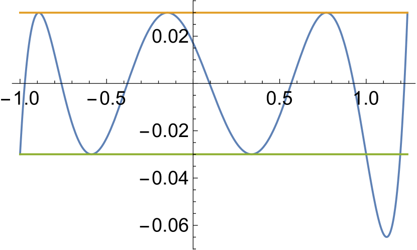
Figure 1: $\widetilde{Z}_{7,t_{0}=-21}$

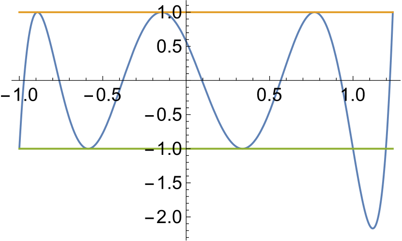
Figure 2: $Z_{7,t_{0}=-21}$

4 Derivation by symbolic computation

It is known from literature (see [11], [12]) that algorithms exist for the parametrization of plane algebraic curves of genus $0$ and $1$, and their implementations are available in computer algebra systems. We will use the algcurves package in Maple. However, as pointed out in [10, p. 179], the defining reduced relation curve $H_{7}(\alpha,\beta)=0$, whose points determine the endpoints of the interval $[\alpha,\beta]$ (to the right of $\boldsymbol{I}$) on which $Z_{7,t}$ also equioscillates, is a genus $4$ curve. Therefore the direct parametrization of the curve $H_{7}=0$, where (see also Formula (7.9) in [30])

$$H_{7}(\alpha,\beta)=$$ (20)

$$(4096-10240\beta^{2}+14080\beta^{4}-9984\beta^{6}+1776\beta^{8}+280\beta^{10}-7\beta^{12})+$$

$$\alpha(12288\beta-13312\beta^{3}+5632\beta^{5}-5760\beta^{7}+1136\beta^{9}+28\beta^{11})+$$

$$\alpha^{2}(-2048+25088\beta^{2}-29952\beta^{4}+10560\beta^{6}-3624\beta^{8}+42\beta^{10})+$$

$$\alpha^{3}(-17408\beta+33792\beta^{3}-19328\beta^{5}+3648\beta^{7}-484\beta^{9})+$$

$$\alpha^{4}(-8448-8448\beta^{2}+23712\beta^{4}-7632\beta^{6}+1311\beta^{8})+$$

$$\alpha^{5}(1536\beta-10624\beta^{3}+11680\beta^{5}-1800\beta^{7})+$$

$$\alpha^{6}(7424-4288\beta^{2}-3472\beta^{4}+1260\beta^{6})+$$

$$\alpha^{7}(4992\beta-4032\beta^{3}-168\beta^{5})+\alpha^{8}(-1040+1976\beta^{2}-441\beta^{4})+$$

$$\alpha^{9}(-144\beta+364\beta^{3})+\alpha^{10}(184-118\beta^{2})+\alpha^{11}12\beta+\alpha^{12},$$

and thus the proposed way in [10] of parametrizing $\widetilde{Z}_{7,t}$ (or $Z_{7,t}$) does not work with the existing implemented algorithms. This is why in [10] the septic case is called a challenge which is subject to further investigation. We remedy this obstacle by the following observation:

Lemma 3.

Certain 2D projections to the coefficient planes of the algebraic space curve $(a_{0,7}(t),\dots,a_{7,7}(t))\subset\mathbb{R}^{8}$ associated to $\widetilde{Z}_{7,t}(x)$, which can be given as a zero-set of $P_{7}(a_{j},a_{k})$, have smaller genuses than the defining reduced relation curve $H_{7}(\alpha,\beta)=0$. In fact, their genuses are determined by the parity of the index-pairs $(j,k),\quad j=0,\dots,5,\,k=j+1,\dots,6$.

Proof.

Using the algcurves package, direct exact computation reveals, for example, that $g(P_{7}(a_{3},a_{5})=0)=1<4$.

To save space, we omit to express the plane projection curve $P_{7}(a_{3},a_{5})$ by formula, which would be a quite bulky one. However, the reader is invited to check the genus computation by recovering $P_{7}(a_{3},a_{5})$ from (21) below, as

$$P_{7}(a_{3},a_{5})\!=\!{\rm res}^{2}_{t}\left({\rm res}^{4}_{o}(r_{31}\!+\!o\,r_{32}\!-\!a_{3}q_{3},o^{2}\!\!-\!\omega^{2}),{\rm res}^{4}_{o}(r_{51}\!+\!o\,r_{52}\!-\!a_{5}q_{5},o^{2}\!\!-\!\omega^{2})\right),$$

where ${\rm res}^{j}_{x}$ denotes the $j$-th factor of the resultant with respect to the variable $x$. ∎

Therefore we use first the known algorithm for the radical parametrizaton of the elliptic curve $P_{7}(a_{3},a_{5})=0$. We compute the Weierstrass normal form and an inverse morphism. After simplification, we so obtain the form given in (21) below:

$$a_{3}=a_{3,7}=a_{3,7}(t)=\frac{r_{31}+\omega r_{32}}{q_{3}}\,\wedge\,a_{5}=a_{5,7}=a_{5,7}(t)=\frac{r_{51}+\omega r_{52}}{q_{5}},$$ (21)

$$\hbox{where }r_{3i}=r_{3i}(t),r_{5i}=r_{5i}(t),q_{3}=q_{3}(t),\hbox{ and }q_{5}=q_{5}(t);\quad i=1,2$$

and

$$r_{31} =-67050634131834282413-65805513145120988466t-$$

$$33209816302438483773t^{2}-8207018843674538160t^{3}+$$

$$61248828418901340t^{4}+573066725434213512t^{5}+$$

$$157302381643747500t^{6}+23037858884482608t^{7}+$$

$$2281318952792298t^{8}+137865778703060t^{9}-7570217151078t^{10}-$$

$$2900985706704t^{11}-249483884148t^{12}-3952502904t^{13}+$$

$$453522684t^{14}+18457680t^{15}+1707483t^{16}-6834t^{17}-5t^{18},$$

$$r_{32} =5715348771948850560+3280169094303556224t+$$

$$482405786587260288t^{2}-71294988953030016t^{3}-$$

$$37631007796747392t^{4}-8178434211316608t^{5}-$$

$$1465523678239872t^{6}-200841049348992t^{7}-16338603726720t^{8}-$$

$$1614798985344t^{9}-380404637568t^{10}-52711585920t^{11}-$$

$$3232979328t^{12}-83650176t^{13}-3459456t^{14}+98688t^{15},$$

$$q_{3} =(-11+t)^{2}(13+t)^{10}(-1763+75t+111t^{2}+t^{3})^{2},$$

$$r_{51} =3(22532652131-4558144146t-7976565369t^{2}-1580832984t^{3}-$$

$$52130250t^{4}+4221396t^{5}+476790t^{6}+87336t^{7}+18279t^{8}-$$

$$1426t^{9}+3t^{10}),$$

$$r_{52} =3(1455149952+337123904t+36161984t^{2}+8501568t^{3}+$$

$$992704t^{4}+51904t^{5}-4800t^{6}+4544t^{7}-64t^{8}),$$

$$q_{5} =(-11+t)^{2}(13+t)^{5}(-1763+75t+111t^{2}+t^{3}).$$

By using the polynomial $Q_{1}(a_{5},\alpha)$ which was derived using Groebner basis computation from the Abel-Pell differential equation (5) by coefficient comparison, and the polynomial $Q_{2}(a_{5},t)$ stemming from the parametrization in (21), and taking the smaller factor of the resultant ${\rm res}_{a_{5}}(Q_{1},Q_{2})$, we obtain

$$Q_{3}(\alpha,t)=\big{(}11243366790769+1414302826044t-1165440897006t^{2}-$$ (22)

$$225646565396t^{3}+38213311311t^{4}+11448834552t^{5}-$$

$$152423364t^{6}-231859656t^{7}-11635425t^{8}+1600204t^{9}+$$

$$138450t^{10}+732t^{11}+t^{12}\big{)}+$$

$$\alpha^{2}\big{(}-22569735604130-3071056384440t+2108952113820t^{2}+$$

$$410418431848t^{3}-47150209566t^{4}-15418665072t^{5}-$$

$$125813496t^{6}+206967312t^{7}+7843842t^{8}-1161176t^{9}-$$

$$36324t^{10}+2184t^{11}-2t^{12}\big{)}+$$

$$\alpha^{4}\big{(}11326363139377+1656707880828t-943672290990t^{2}-$$

$$185096942420t^{3}+8526067407t^{4}+3636819576t^{5}+109344444t^{6}-$$

$$23639112t^{7}-1673505t^{8}+24844t^{9}+5394t^{10}+156t^{11}+t^{12}\big{)}.$$

This is obviously a quadratic expression of $\alpha^{2}$ and thus $\alpha$ can be expressed in terms of the parameter $t$ by radicals, i.e., $\alpha=\alpha(t)$. Similarly, it turns out that in this way we also obtain a nonsimple radical parametrization for $\beta$ and $s$ in the form of $\beta(t)$ and $s(t)$, see (23) below:

$$\alpha(t)=\sqrt{\frac{pa_{1}+pa_{2}\omega}{q_{5}}},\,\beta(t)=\sqrt{\frac{pb_{1}+pb_{2}\omega}{q_{5}}},\,s(t)=\frac{1}{7}\sqrt{\frac{ps_{1}+ps_{2}\omega}{q_{5}}},$$ (23)

$$\hbox{where }pa_{i}=pa_{i}(t),pb_{i}=pb_{i}(t),ps_{i}=ps_{i}(t);\quad i=1,2$$

and

$$pa_{1}= -78915159455-11841667910t+6656486445t^{2}+1445318328t^{3}-$$

$$98097774t^{4}-45176292t^{5}-1757742t^{6}+383160t^{7}+20493t^{8}-$$

$$1094t^{9}+t^{10},$$

$$pa_{2}= -32(-237047-688048t-631196t^{2}-136576t^{3}+52510t^{4}+$$

$$7760t^{5}-1292t^{6}-160t^{7}+t^{8}),$$

$$pb_{1}= -83889211967-23402064230t-1593364563t^{2}-238787016t^{3}-$$

$$84657966t^{4}-8058276t^{5}+964434t^{6}+8760t^{7}+5229t^{8}+$$

$$154t^{9}+t^{10},$$

$$pb_{2}= \,\,55296(2153+4729t+3002t^{2}+434t^{3}+13t^{4}+5t^{5}),$$

$$ps_{1}= -430297163879-140961934838t-23363774235t^{2}-$$

$$3595306632t^{3}-594107646t^{4}-113195268t^{5}-1046526t^{6}+$$

$$1347960t^{7}+171621t^{8}-10742t^{9}+25t^{10},$$

$$ps_{2}= -96(-94197721-28304354t-6941146t^{2}-1190186t^{3}-19228t^{4}+$$

$$154t^{5}-310t^{6}-398t^{7}+5t^{8}).$$

By using the polynomials from the Groebner basis, formulae can be derived for $a_{1,7}(t)$ (similar to $a_{3,7}(t)$ and $a_{5,7}(t)$ in (21)) and for the even-indexed coefficents $a_{0,7}(t)$, $a_{2,7}(t)$, $a_{4,7}(t)$ and for $L_{7}(t)$ (similar to $s(t)$ in (23)), so that we can determine, for $n=7$, the monic polynomial in (3), with $a_{6,7}(t)=-7s(t)$ and $a_{7,7}(t)=1$. But we omit these coefficient-formulae in order to save space, since they can be recovered from Theorem 1. In fact, since $-L_{7}(t)=\widetilde{Z}_{7,t}(1)=1+\sum_{k=0}^{6}a_{k}(t)$, it follows from $Z_{7,t}(x)=\widetilde{Z}_{7,t}/L_{7}(t)$ that for the coefficients of $Z_{7,t}$ there holds $b_{k,7}(t)=a_{k,7}(t)/L_{7}(t)$, in particular $b_{7,7}(t)=1/L_{7}(t)$.

In this way we have obtained our radical parametrization of the septic normalized proper Zolotarev polynomials $Z_{7,t}$ in Theorem 1.

As for the parameter interval $I_{7}$, we first determine the possible real parameter values $t$ for which

$$a_{3,7}(t)={\rm Root[}25621-21445x-3609x^{2}+x^{3},2{\rm]}\,\,\wedge$$ (24)

$$a_{5,7}(t)={\rm Root[}2443+651x-343x^{2}+x^{3},1{\rm]}$$

holds, where the right hand sides of the above equations are the coefficients of the monic version of the limiting polynomial in (10). We obtain the unique solution $\theta={\rm Root[}-1847-93x+27x^{2}+x^{3},1{\rm]}$. Second, using the expected range $(a_{3,7}(\theta),19/16)\times(-2,a_{5,7}(\theta))$ for $(a_{3,7}(t),a_{5,7}(t))$, we conclude that the only appropriate choice for $I_{7}$ is $(\theta,-13)$ as given in Theorem 1. ∎

Example 4.

We again prescribe $t=t_{0}=-21\in I_{7}$, which corresponds to prescribe $s(t_{0})=s_{0}\in\left(\tan^{2}(\frac{\pi}{14}),\infty\right)=(0.0520950836\dots,\infty)$, and get for $L_{7}(t_{0})$, $s(t_{0})$, $\alpha$, $\beta$, $\gamma=\frac{\alpha+\beta}{2}-s(t_{0})\,$the concrete values

$$L_{7}(t_{0})= \frac{6591796875}{1024\sqrt{2(11553696783009431\!+\!4716776960201434\sqrt{6})}}=$$

$$0.0299442459\ldots$$ (25)

$$s(t_{0})=\frac{1}{28}\sqrt{\frac{-24764015+10110318\sqrt{6}}{142}}=0.0996381277\ldots$$ (26)

$$\alpha(t_{0})=\alpha=\frac{1}{4}\sqrt{\frac{-1816103+742750\sqrt{6}}{142}}=1.1970302256\ldots$$ (27)

$$\beta(t_{0})=\beta=\frac{1}{4}\sqrt{\frac{-330503+136350\sqrt{6}}{142}}=1.2384903969\ldots$$ (28)

$$\gamma(t_{0})=\gamma=\frac{1}{7}\sqrt{\frac{-2665+1138\sqrt{6}}{2}}=1.1181221834\ldots\,.\,\qed$$ (29)

Example 5.

The goal is to solve ZFP (2) for $n=7$ and for $s=s_{0}=2>\tan^{2}(\frac{\pi}{14})$, say. To this end, we replace in (23) the left-hand side $s(t)$ by $2$ and solve the corresponding equation for the variable $t$, where the unique solution from $I_{7}$ reads $t=t_{0}={\rm Root[}u_{12}(x),2{\rm]}=-13.0305732483\ldots\,$, with

$$u_{12}(x)=$$ (30)

$$45678110765558881+6234622186059196x-4142454922929870x^{2}-$$

$$804497641938708x^{3}+33981103268895x^{4}+15022950168312x^{5}+$$

$$496259775228x^{6}-87343156680x^{7}-6119479377x^{8}-32085428x^{9}+$$

$$16838386x^{10}+1138140x^{11}+3249x^{12}.$$

Then we insert this $t_{0}$ into $\frac{Z_{7,t}(x)}{b_{7,7}(t)}$ to obtain

$$\widetilde{Z}_{7,t_{0}}(x)=\widetilde{Z}_{7,s_{0}}^{*}(x)=$$ (31)

$$0.4369440905\ldots+(-0.1873410678\ldots)x+(-7.8705484829\ldots)x^{2}+$$

$$(1.1870230011\ldots)x^{3}+(20.9955470665\ldots)x^{4}+(-1.9996819333\ldots)x^{5}+$$

$$(-14)x^{6}+x^{7}.$$

This means that $\min_{(a_{0,7},\cdots,a_{5,7)}\in\mathbb{R}^{6}}||P_{7}||_{\infty}=||\widetilde{Z}_{7,t_{0}}||_{\infty}=||\widetilde{Z}_{7,s_{0}}^{*}||_{\infty}=L_{7}(t_{0})=L_{7}(s_{0})$ where $P_{7}(x)=\sum_{k=0}^{5}a_{k,7}x^{k}+(-14)x^{6}+x^{7}$, i.e. its first two leading coefficients are prescribed. Evaluating $L_{7}(t)=\frac{1}{b_{7,7}(t)}$ at $t=t_{0}$ (see (1)), gives $L_{7}(t_{0})=0.4380573257\ldots$  .∎

5 A note on the equations of Abel-Pell and Peherstorfer-Schiefermayr for $n=7$

The Abel-Pell differential equation for $Z_{7,t}$ reads, see (5), (1), (23),

$$\frac{(1-x^{2})(x-\alpha(t))(x-\beta(t))(Z_{7,t}\,^{\prime}(x))^{2}}{49(x-\gamma(t))^{2}}+(Z_{7,t}(x))^{2}=1.$$ (32)

Since all terms are defined for $n=7$, a simplification with Maple or Mathematica will confirm that (32) holds true. For the special parameter value $t=t_{0}=-21$ a verification of (32) can be carried out by using (11)–(19) and (26)–(29).

The Peherstorfer-Schiefermayr system of nonlinear equations (6)–(7) reads, for $n=7$,

$$\alpha(t)+\beta(t)+2(z_{1}+z_{2}+z_{3}+z_{4}+z_{5})-14s(t)=0$$ (33)

$$(-1)^{k}+2(-z_{1}^{k}+z_{2}^{k}-z_{3}^{k}+z_{4}^{k}-z_{5}^{k})+1+(\alpha(t))^{k}-(\beta(t))^{k}=0\,(k=1,\dots,6).$$ (34)

The equioscillation points $z_{2}$ and $z_{4}$, where $Z_{7,t}(z_{2})=Z_{7,t}(z_{4})=-1$ and $Z_{7,t}^{\prime}(z_{2})=Z_{7,t}^{\prime}(z_{4})=0$ holds, can be given in an explicit form as follows:

$$z_{2}=z_{2}(t)=$$ (35)

$$\!-\!\sqrt{\frac{(t\!-\!11)p_{9}\!-\!16\omega(1+t)^{2}p_{6}\!+\!8(1+t)^{2}(13+t)\sqrt{3(11\!-\!t)(p_{12}\!-\!2\omega p_{10})}}{q_{5}}},$$

$$z_{4}=z_{4}(t)=$$ (36)

$$\sqrt{\frac{(t\!-\!11)p_{9}\!-\!16\omega(1+t)^{2}p_{6}\!-\!8(1+t)^{2}(13+t)\sqrt{3(11\!-\!t)(p_{12}\!-\!2\omega p_{10})}}{q_{5}}},$$

where

$$p_{9}=p_{9}(t)=$$

$$7458346453+2414057145t+80738436t^{2}-35137404t^{3}+$$

$$943590t^{4}+1460238t^{5}+136212t^{6}+4020t^{7}-339t^{8}+t^{9},$$

$$p_{6}=p_{6}(t)=$$

$$-4757750-991641t+35097t^{2}+1478t^{3}-84t^{4}-93t^{5}+t^{6},$$

$$p_{12}=p_{12}(t)=$$

$$9627927080284+4974116032425t+1038680780799t^{2}+$$

$$126082292719t^{3}+6771588669t^{4}+996190362t^{5}+407573430t^{6}+$$

$$26107902t^{7}-4154346t^{8}-474323t^{9}+59547t^{10}-861t^{11}+t^{12},$$

$$p_{10}=p_{10}(t)=$$

$$122595778519+52782140344t+8848501713t^{2}+1458683184t^{3}+$$

$$201606006t^{4}+6367392t^{5}-2103342t^{6}-42288t^{7}+68355t^{8}-$$

$$2648t^{9}+13t^{10}.$$

The equioscillation points $z_{1},z_{3}$ and $z_{5}$ where $Z_{7,t}(z_{1})=Z_{7,t}(z_{3})=Z_{7,t}(z_{5})=1$ and $Z_{7,t}^{\prime}(z_{1})=Z_{7,t}^{\prime}(z_{3})=Z_{7,t}^{\prime}(z_{5})=0$ holds, can be represented in a similar but more bulky form (as solutions of a cubic polynomial equation with casus irreducibilis) and are omitted.

For the special parameter value $t=t_{0}=-21$ a verification of (33), (34) can be carried out by using $s(t_{0})$, $\alpha$ and $\beta$ from (26)–(28) and the following identities:

$$z_{1}=-\sqrt{\tau_{3}}=-0.8914485687\ldots,\hbox{ where }\tau_{3}={\rm Root[}u_{3}(x),3{\rm]}\hbox{ and}$$ (37)

$$u_{3}(x)=-150\sqrt{6}(568552997+66091829356x+136570772x^{2})+$$

$$208899235967+24283711656924x+50114778876x^{2}+45812608x^{3}$$

$$z_{2}=\!\!-\frac{1}{8}\sqrt{\frac{1}{71}(\!-1744831\!\!+\!\!712750\sqrt{6}\!\!+\!\!25\sqrt{2104102185\!-\!858995940\sqrt{6}}}\!=$$ (38)

$$\hskip 256.0748pt-0.5873784916\ldots$$

$$z_{3}=-\sqrt{\tau_{1}}=-0.1483533115\ldots,\hbox{ where }\tau_{1}={\rm Root[}u_{3}(x),1{\rm]}$$ (39)

$$z_{4}=\!\!\frac{1}{8}\sqrt{\frac{1}{71}(\!-1744831\!+\!712750\sqrt{6}\!-\!25\sqrt{2104102185\!-\!858995940\sqrt{6}}}=$$ (40)

$$\hskip 273.14662pt{0.3375968260\ldots}$$

$$z_{5}=\sqrt{\tau_{2}}=0.7692901289\ldots,\hbox{ where }\tau_{2}={\rm Root[}u_{3}(x),2{\rm]}.$$ (41)

6 Concluding remarks

Remark 6.

The obtained septic radical parametrization in Theorem 1 which is similar to, but more complicated than the one for $n=5$ in [10] and for $n=6$ in [31], may possibly be further simplified. To find a re-parametrization for $n=7$ is subject to further investigations.

Remark 7.

A systematic computation of the genuses of all possible plane projection curves $P_{n}(a_{j},a_{k})=0$ of the proper Zolotarev polynomials $\widetilde{Z}_{n,t}$ and $Z_{n,t}$ for $n>4$ would shed a light on the structure of the associated space curves.

Remark 8.

The only parameter constellation $t\in I_{7}$ where $\widetilde{Z}_{7,t}=Z_{7,t}$ holds is $t=t_{0}=-13.0058608055\ldots$ (which is the root of an integer polynomial of degree 56) since then $b_{7,7}(t)=1$ holds.