Simultaneous Skull Conductivity and Focal Source Imaging from EEG Recordings with the help of Bayesian Uncertainty Modelling

Abstract

The electroencephalography (EEG) source imaging problem is very sensitive to the electrical modelling of the skull of the patient under examination. Unfortunately, the currently available EEG devices and their embedded software do not take this into account; instead, it is common to use a literature-based skull conductivity parameter. In this paper, we propose a statistical method based on the Bayesian approximation error approach to compensate for source imaging errors due to the unknown skull conductivity and, simultaneously, to compute a low-order estimate for the actual skull conductivity value. By using simulated EEG data that corresponds to focal source activity, we demonstrate the potential of the method to reconstruct the underlying focal sources and low-order errors induced by the unknown skull conductivity. Subsequently, the estimated errors are used to approximate the skull conductivity. The results indicate clear improvements in the source localization accuracy and feasible skull conductivity estimates.

1 Introduction

The estimation of the focal brain activity from electroencephalography (EEG) data is an ill-posed inverse problem, and the solution depends strongly on the accuracy of the head model, particularly the used skull conductivity value [1, 2]. The skull conductivity value can be calibrated by using well defined somatosensory evoked potentials / fields in combination with EEG [3], combined EEG/MEG [4] or by using electrical impedance tomography (EIT) -based techniques [5]. However, these methods are sometimes unreliable, computationally effortful and may require auxiliary imaging tools.

In our previous studies [6, 7], we demonstrated a more straightforward approach that was based on uncertainty modelling via the Bayesian approximation error (BAE) approach [8]. With BAE, the natural variability of the skull conductivity was modelled in a probability distribution, and subsequently its effects on the EEG data were taken statistically into account in the observation model (likelihood) with the help of an additive modelling error term. This allowed us to use an approximate skull conductivity in the EEG source imaging, i.e. to neglect the calibration step completely, and still get feasible source configuration estimates.

In this paper, we demonstrate with simulations that in addition to the source configuration the Bayesian uncertainty modelling also allows simultaneous estimation of the unknown skull conductivity. This estimation can be carried out through a low order decomposition of the modelling error term [8, 9].

We envision that the proposed approach could be used as such, or alternatively as a calibration step to determine the skull conductivity of a patient. The benefit compared to current injection -based techniques is that it relies solely on EEG data and thus avoids the requirement for a brain rest period before the actual EEG examination. In addition, this approach does not add computational effort (to the regular source imaging) since it does not involve non-linear formulations or unstable matrix inversions [3, 10]; instead, all the required pre-computations can be performed off-line before any experiments take place.

2 Theory

2.1 Bayesian framework with linear forward model

The computational domain is denoted with $\Omega$ and its electric conductivity with $\sigma(x)$ where $x\in\Omega$. The numerical observation model is

$$v=A(\sigma)d+e,$$ (1)

where $v\in\mathbb{R}^{m}$ are the measurements, $m$ is the number of measurements, $A(\sigma)\in\mathbb{R}^{m\times 2n}$ is the (2-dimensional) lead field matrix that depends on $\sigma$, $d\in\mathbb{R}^{2n}$ is the distributed dipole source configuration and $e\sim\mathcal{N}(e_{*},\Gamma_{e})$ is the measurement noise. Note that here the model $A(\sigma)$ assumes (unrealistically) that the accurate values of electric conductivities are known.

In the Bayesian framework, the inverse solution is the posterior density

$$\pi(d|v)\propto\pi(v|d)\pi(d),$$ (2)

where $\pi(v|d)$ is the likelihood and $\pi(d)$ the prior.

For the model (1), the likelihood can be written as

$$\pi(v|d)\propto\exp\Big{(}-\frac{1}{2}(v-A(\sigma)d-e_{*})^{\mathrm{T}}\Gamma_{e}^{-1}(v-A(\sigma)d-e_{*})\Big{)}.$$ (3)

2.2 Bayesian approximation error (BAE) approach

In BAE, the accurate lead field matrix $A(\sigma)$ is replaced with an approximate (standard) lead field matrix $A_{0}=A(\sigma_{0})$ in which fixed electric conductivities $\sigma_{0}$ are used. Now, the observation model (1) can be written as

$$v=A_{0}d+\varepsilon+e$$ (4)

where

$$\varepsilon=A(\sigma)d-A_{0}d$$ (5)

is the induced approximation error, $\varepsilon\in\mathbb{R}^{m}$.

In order to approximate the unknown skull conductivity, we need to obtain an estimate about the approximation error. Similarly as in [9, 8], we express $\varepsilon$ as a linear combination of basis functions. Numerically, the estimation of $\varepsilon$ is tractable if most of its variance is captured in only few of the decomposition terms [9, 8].

A feasible set of basis functions that assigns most of the variance of $\varepsilon$ in the first few terms can be chosen based on the eigenvalue decomposing of the modelling error covariance $\Gamma_{\varepsilon}=\mathbb{E}[(\varepsilon-\varepsilon_{*})(\varepsilon-\varepsilon_{*})^{\mathrm{T}}]$. In particular, $\Gamma_{\varepsilon}$ can be decomposed according to

$$\Gamma_{\varepsilon}=\Sigma_{k=1}^{m}\lambda_{k}w_{k}w_{k}^{\mathrm{T}},$$ (6)

where $\lambda_{k}\in\mathbb{R}^{m}$ are the eigenvalues and $w_{k}\in\mathbb{R}^{m}$ are the eigenvectors of $\Gamma_{\varepsilon}$. Based on this decomposition, we have that $\varepsilon-\varepsilon_{*}\;\in\;\mathrm{span}\{w_{1},\ldots,w_{k}\}$.

The approximation error can be expressed as

$$\varepsilon=\varepsilon_{*}+\varepsilon^{\prime}+\varepsilon^{\prime\prime},$$ (7)

where $\varepsilon^{\prime}=\Sigma_{k=1}^{p}\alpha_{k}w_{k}$ and $\varepsilon^{\prime\prime}=\Sigma_{j=p+1}^{m}\beta_{j}w_{j}$, with $\mathbb{E}[\varepsilon^{\prime}]=0$ and $\mathbb{E}[\varepsilon^{\prime\prime}]=0$. The coefficients $\alpha_{k}$ and $\beta_{j}$ are given by the inner products $\alpha_{k}=<\varepsilon-\varepsilon_{*},w_{k}>$ and $\beta_{j}=<\varepsilon-\varepsilon_{*},w_{j}>$.

Thus, the observation model (4) can be rewritten as

$$v=A_{0}d+\varepsilon_{*}+W\alpha+\varepsilon^{\prime\prime}+e,$$ (8)

where $\varepsilon^{\prime}=W\alpha$, $W=[w_{1},w_{2},...,w_{p}]\in\mathbb{R}^{m\times p}$ contains the first $p$ eigenvectors and $\alpha=(\alpha_{1},\alpha_{2},...,\alpha_{p})^{\mathrm{T}}\in\mathbb{R}^{p}$. Note that $\varepsilon^{\prime\prime}=Q\beta=QQ^{\mathrm{T}}\varepsilon$ where $Q=[w_{p+1},\ldots,w_{m}]\in\mathbb{R}^{(m-p)\times m}$.

For the simultaneous estimation of $d$ and $\alpha$, we have to construct the posterior model $\pi(d,\alpha|v)$. To obtain a computationally efficient solution, we make the technical approximation that $(d,\alpha,e,\varepsilon^{\prime\prime})$ are mutually Gaussian and uncorrelated [9, 8]. Then, we obtain the approximate likelihood

$$\tilde{\pi}(v|d,\alpha)\propto\exp\Big{(}-\frac{1}{2}(v-A_{0}d-\varepsilon_{*}-W\alpha-e_{*})^{\mathrm{T}}$$

$$\qquad(\Gamma_{\varepsilon^{\prime\prime}}+\Gamma_{e})^{-1}(v-A_{0}d-\varepsilon_{*}-W\alpha-e_{*})\Big{)},$$ (9)

where $\Gamma_{\varepsilon^{\prime\prime}}=\Sigma_{p+1}^{m}\lambda_{j}w_{j}w_{j}^{\mathrm{T}}$. Based on the eigenvalue decomposition and the Gaussian approximations, we have that the coefficients $\alpha$ are normally distributed with zero mean and covariance $\Gamma_{\alpha}=\mathrm{diag}(\lambda_{1},\ldots,\lambda_{p})$ (where $\lambda_{1}>\ldots>\lambda_{p}$). Thus, the posterior density becomes

$$\tilde{\pi}(d,\alpha|v)\propto\mathrm{exp}\left(-\frac{1}{2}L_{\varepsilon^{\prime\prime}+e}\|v-A_{0}d-W\alpha-\varepsilon_{*}-e_{*}\|_{2}^{2}\right)\mathrm{exp}\left(-\frac{1}{2}L_{\alpha}\|\alpha\|_{2}^{2}\right)\;\pi(d),$$ (10)

where the Cholesky factors are $(\Gamma_{\varepsilon^{\prime\prime}}+\Gamma_{e})^{-1}=L_{\varepsilon^{\prime\prime}+e}^{\mathrm{T}}L_{\varepsilon^{\prime\prime}+e}$ and $\Gamma_{\alpha}^{-1}=L_{\alpha}^{\mathrm{T}}L_{\alpha}$.

3 Methods

3.1 Head models

A 2-dimensional finite element (FE) -based three compartment (scalp, skull and brain) head model with 32 electrodes was used in the demonstrations (see, Figure 1). For the forward simulations and inverse estimations two different meshes with 2518 and 1780 nodes were constructed, respectively, with source spaces covering the gray matter of the brain.

In particular, we created $K=400$ head models with skull conductivity samples $\sigma^{(k)}$ drawn from a Gaussian distribution $\pi(\sigma)$ with mean $\sigma_{*}=0.0073$ (in S/m) and standard deviation 0.0013 (see, Figure 1). We refer to these head models as sample head models. This skull conductivity distribution coincides with the literature values that range between 0.0041 and 0.033 [11, 12, 4]. The electric conductivity of the scalp was 0.43 [13] and the brain 0.33 [13]. We also created a standard head model with skull conductivity $\sigma_{0}=0.0085$.

3.2 Computation of the approximation error statistics

The approximation error (5) depends both on the skull conductivity and the dipole source location. Feasible estimates for the skull conductivity can be expected if most of the variance of $\varepsilon$ is related to the skull uncertainty. Therefore, we isolated the effect that the skull has on the observations. To do that, we estimated the error statistics for each dipole location separately. In the following text, the subscript $i$ denotes a specific dipole location.

The samples for the error statistics at location $i$ were created by first choosing randomly one of the sample head models and evaluating both the sample model and the standard model with the same single dipole source $d_{i}^{(s)}$, i.e.

$$\varepsilon^{(j)}_{i}=A(\sigma^{(k)}){d}_{i}^{(s)}-A_{0}d_{i}^{(s)}.$$ (11)

A set of $S=1000$ single radial dipole samples $d_{i}^{(s)}$ with varying amplitudes were drawn from a Gaussian distribution $\pi(d_{i})$ with mean 1 and standard deviation 0.01, and 200 different leadfield matrices were used to estimate the error statistics at location $i$. Superscript $j=s+S(k-1)$ where $s=1,\ldots,S$ and $k=1,\ldots K$. The mean $\varepsilon_{i*}$ and error covariance $\Gamma_{\varepsilon_{i}}$ at location $i$ were

$$\varepsilon_{i*}=\frac{\sum_{j=1}^{J}{\varepsilon}_{i}^{(j)}}{J}\,\,\mbox{and}\,\,\Gamma_{\varepsilon_{i}}=\frac{1}{J-1}\sum_{j=1}^{J}(\varepsilon_{i}^{(j)}-\varepsilon_{i*})(\varepsilon_{i}^{(j)}-\varepsilon_{i*})^{\mathrm{T}}.$$ (12)

Samples $\alpha_{i}^{(j)}$ and $\varepsilon_{i}^{\prime\prime(j)}$ were evaluated according to $\alpha_{i}^{(j)}=W_{i}^{\mathrm{T}}(\varepsilon_{i}^{(j)}-\varepsilon_{i*})$ and $\varepsilon_{i}^{\prime\prime(j)}=Q_{i}Q_{i}^{\mathrm{T}}(\varepsilon_{i}^{(j)}-\varepsilon_{i*})$, where $W_{i}$ and $Q_{i}$ were matrices with columns the first $p$ and remaining eigenvectors of $\Gamma_{\varepsilon_{i}}$ respectively.

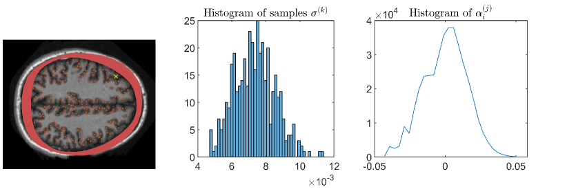
Figure 1: Left: The 2-dimensional human head model used in the computations was segmented in scalp, skull (illustrate with solid red color) and brain compartments. The source space locations are illustrated with red dots. Middle: Histogram of 400 skull conductivity samples. Right: To sample $\alpha$, first a source location (shown with a yellow cross on the left) and 1000 amplitude values for the source are drawn, then sample lead fields (based on the 400 skull conductivities) are used to compute the corresponding approximation errors. The resulting histogram of the first $\alpha$ parameter ($k=1$) has approximately Gaussian form.

3.3 Simultaneous skull conductivity and source estimation

In this work, we compute the maximum a posteriori (MAP) estimates of the posterior (10). Since we study only single dipole source cases, we can use a modified single dipole scan algorithm and solve

$$\begin{bmatrix}\hat{d}_{i}\\ \hat{\alpha}_{i}\end{bmatrix}:=\begin{bmatrix}L_{\varepsilon_{i}^{\prime\prime}+e}A_{0}^{i}&L_{\varepsilon_{i}^{\prime\prime}+e}W_{i}\\ \mathbf{0}&L_{\alpha_{i}}\end{bmatrix}^{-1}\begin{bmatrix}L_{\varepsilon_{i}^{\prime\prime}+e}(v-\varepsilon_{i*}-e_{*})\\ 0\end{bmatrix},\;\;\;\mbox{for }i=1,\ldots,n,$$ (13)

where $n$ is the total number of source locations, $A_{0}^{i}=[A_{0x}^{i}A_{0y}^{i}]$ are the columns of the (standard) leadfield matrix corresponding to location $i$, $\hat{d}_{i}=(d_{x_{i}},d_{y_{i}})$ is the dipole reconstructed at location $i$, $W_{i}\in\mathbb{R}^{m\times p}$ are the basis functions obtained from the eigenvalue decomposition of the error covariance $\Gamma_{\varepsilon_{i}}\in\mathbb{R}^{m\times m}$, $\alpha_{i}\in\mathbb{R}^{p}$ are the reconstructed coefficients for these basis functions, and $L_{\alpha_{i}}=\frac{1}{2}\mathrm{diag}(\lambda_{1}^{-1},\lambda_{2}^{-1},...,\lambda_{p}^{-1})$ where $\lambda$ parameters are the eigenvalues of the covariance $\Gamma_{\varepsilon_{i}}$ (12). The number of $\alpha$ parameters, as well as, the number of eigenvalues (used in the estimates) was defined based on the minimum value $p$ that satisfied $\frac{\sum_{k=1}^{p}\lambda_{k}}{\sum_{k=1}^{m}\lambda_{k}}\geq 0.85$. In most cases, either one or two $\lambda$ parameters were needed.

The solution is the pair

$$(\hat{d}_{l},\hat{\alpha}_{l})\leftarrow\min_{i=1:n}\{\|L_{\varepsilon_{i}^{\prime\prime}+e}(v-A_{0}^{i}\hat{d}_{i}-\varepsilon_{i*}-W_{i}\hat{\alpha}_{i}-e_{*})\|_{2}^{2}+L_{\alpha_{i}}\|\hat{\alpha}_{i}\|_{2}^{2}\}$$ (14)

where $i=l$ is the location that gives the lowest value for the functional (14).

Given the dipole location $l$, the approximation error (5) can be written as

$$\varepsilon_{l}=A^{l}(\sigma)d_{l}-A_{0}^{l}d_{l},$$ (15)

where $\varepsilon_{l}=W_{l}\alpha_{l}$.

The skull conductivity can now be estimated by maximizing

$$\hat{\sigma}:=\max_{\sigma}\pi(\sigma|\alpha_{l}).$$ (16)

The conditional probability distribution $\pi(\sigma|\alpha_{l})$ is

$$\pi(\sigma|\alpha_{l})=\int\pi(\sigma,d_{l}|\alpha_{l})\;\mathrm{d}d_{l}\propto\pi(\sigma)\int\pi(\alpha_{l}|\sigma,d_{l})\pi(d_{l})\;\mathrm{d}d_{l},$$ (17)

where $\sigma$ and $d_{l}$ are mutually independent.

From equation (15), we have that $\int\pi(\alpha_{l}|\sigma,d_{l})\pi(d_{l})\;\mathrm{d}d_{l}=\int\delta(W_{l}\alpha_{l}-[A^{l}(\sigma)-A_{0}^{l}]d_{l})\pi(d_{l})\;\mathrm{d}d_{l}=\frac{1}{|f_{l}^{-1}(\sigma)|}\pi_{d_{l}}(f_{l}(\sigma)\alpha_{l})$ where the subscript $d_{l}$ is used to clarify that this is the probability density of $d_{l}$, and the expression $f_{l}(\sigma)$ formally comes from the inversion of the lead field matrix difference and multiplication with $W_{l}$. So, $\pi(\sigma|\alpha_{l})\propto\pi(\sigma)\;\frac{1}{|f_{l}^{-1}(\sigma)|}\pi_{d_{l}}(f_{l}(\sigma)\alpha_{l})$. Even though $\pi(\sigma)$ an $\pi_{d_{l}}(.)$ have been modelled as Gaussian distributions, the non-linearity with respect to $\sigma$ and often the infeasibility of estimating $f_{l}(\sigma)$ can prohibit a straightforward $\sigma$ estimation. Instead we can use $\pi(\sigma|\alpha_{l})\propto\pi(\sigma,\alpha_{l})$.

Since, $\pi(\sigma,\alpha_{l})=\frac{1}{|f_{l}^{-1}(\sigma)|}\pi(\sigma)\;\pi_{d_{l}}(f_{l}(\sigma)\alpha_{l})$, the joint distribution of $\sigma$ and $\alpha_{l}$ can be approximated as Gaussian, and therefore the MAP estimate (16) gives

$$\hat{\sigma}=\sigma_{*}+\Gamma_{\sigma\alpha_{l}}\Gamma_{\alpha_{l}}^{-1}\hat{\alpha}_{l},$$ (18)

where $\hat{\alpha}_{l}$ is the solution of problem (14), $\sigma_{*}$ is the mean value of the postulated skull conductivity distribution, $\Gamma_{\sigma\alpha_{l}}$ is the cross-covariance between $\sigma$ and $\alpha_{l}$ (estimated using samples $\alpha_{l}^{(j)}$ and $\sigma^{(k)}$ as described in section 3.2), and $\Gamma_{\alpha_{l}}=\mathrm{diag}(\lambda_{1},\ldots,\lambda_{p})$ where $\lambda_{p}$ are the first $p$ eigenvalues of the sampled-based error covariance $\Gamma_{\varepsilon_{l}}$ (12).

4 Results, discussion and future work

To demonstrate the simultaneous dipole and skull conductivity reconstruction, we used two test cases with different skull conductivities. The EEG data was computed using the accurate model that had either skull conductivity 0.0055 or 0.011 S/m, a single radial dipole source, and signal to noise ratio 30 dB. In Figure 2, we show first the test set-up, then the dipole-scan reconstruction with the standard lead field that has skull conductivity 0.0085 S/m, and finally the proposed Bayesian error modelling result. To ease comparisons, we calculated the Euclidean distance (ED) (in milli meters) between the actual and reconstructed source. It can be seen that the proposed uncertainty modelling improves the source reconstructions when compared to the solution of the standard model. Moreover, the estimates for the skull conductivity are close to the true skull conductivities.

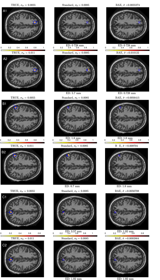
Figure 2: Left column: Test cases with three different source locations and two different skull conductivity values, either lower (0.0055 S/m) or higher (0.011 S/m) than the standard skull conductivity (0.0085 S/m). The blue circle and the line represent the true location and direction of the dipole source, respectively. Middle column: Source reconstruction results when the standard skull conductivity was used in the lead field. The ED values give the Euclidean distance between the true and reconstructed source. The true location is denoted with a blue cross. Right column: Simultaneous skull conductivity and source location reconstructions with the proposed Bayesian uncertainty modelling approch. As can be seen, the proposed approach improves the source localization compared to the results with the standard model and additionally achieves to estimate the skull conductivity.

The feasibility of the skull conductivity estimates depends on how well the first few eigenvectors of $\Gamma_{\varepsilon}$ describe the conductivity related modelling errors. In the future, we aim to isolate the conductivity related errors from other error sources (e.g. discretization) in order to improve the skull conductivity estimates.

In our analysis the head geometry was considered fully known; however, it can also be taken into account as an uncertainty [14]. We also note that in this work we estimated a single conductivity value for the whole skull. As a next step, we plan to use the proposed approach in conjugation with other optimization techniques [15, 16] to produce more detailed skull conductivity maps.

5 Conclusion

We have demonstrated that with the help of the Bayesian uncertainty modeling the EEG source imaging problem could be reformulated in such a way that it allows to estimate, simultaneously with the source configuration, a low-order approximation for the modelling error. With the help of this modelling error estimate, the underlying skull conductivity could be reconstructed.

Conflict of interest

The authors declare that they have no conflicts of interest.

References

- [1] B. Vanrumste, G.V. Hoey, R.V. de Walle, M. D’Have, I. Lemahieu, P. Boon, Med. Biol. Eng. Comput. 38(5), 528 (2000).
- [2] M. Dannhauer, B. Lanfer, C. Wolters, T. Knösche, Hum. Brain Mapp. 32, 1383 (2011)
- [3] S. Lew, C.H. Wolters, A. Anwander, S. Makeig, R.S. MacLeod, Hum. Brain Mapp. 30(9), 2862 (2009).
- [4] U. Aydin, J. Vorwerk, P. Küpper, M. Heers, H. Kugel, A. Galka, L. Hamid, J. Wellmer, C. Kellinghaus, S. Rampp, C.H. Wolters, PLoS ONE 9, e93154 (2014)
- [5] S.I. Goncalves, J.C. de Munck, J.P. Verbunt, R.M. Heethaar, F.H. da Silva, IEEE Trans. Biomed. Eng. 50(9), 1124 (2003)
- [6] V. Rimpiläinen, A. Koulouri, F. Lucka, J.P. Kaipio, C.H. Wolters, IFMBE Proc. 65, 892 (2018)
- [7] V. Rimpiläinen, A. Koulouri, F. Lucka, J.P. Kaipio, C.H. Wolters, NeuroImage 188, 252 (2019).
- [8] J. Kaipio, V. Kolehmainen, in Bayesian Theory and Applications, ed. by P. Damien, N. Polson, D. Stephens (Oxford University Press, 2013)
- [9] A. Nissinen, V. Kolehmainen, J.P. Kaipio, Int. J. Uncertain. Quantif. 1(3), 203 (2011)
- [10] C. Papageorgakis, Patient specific conductivity models: characterization of the skull bones. Ph.D. thesis (2017)
- [11] R. Hoekema, G.H. Wieneke, C.W. van Veelen, P.C. van Rijen, G.J. Huiskamp, J. Ansems, A.C. van Huffelen, Brain Topogr. 16(1), 29 (2003)
- [12] S. Homma, T. Musha, Y. Nakajima, Y. Okomoto, S. Blom, R. Flink, K.E. Hagbarth, Neurosci. Res. 22(1), 51 (1995)
- [13] C. Ramon, P.H. Schimpf, J. Haueisen, Biomed. Eng. Online 5(10) (2006)
- [14] A. Koulouri, V. Rimpiläinen, M. Brookes, J.P. Kaipio, Appl. Num. Math. 106, 24 (2016)
- [15] Z.A. Acar, C.E. Acar, S. Makeig, NeuroImage 124, 168 (2016).
- [16] F. Costa, H. Batatia, T. Oberlin, J.Y. Tourneret, arXiv: 1609.06874 (2016)