Chiral Condensate and Spectral Density at full five-loop and partial six-loop orders of Renormalization Group Optimized Perturbation

Abstract

We reconsider our former determination of the chiral quark condensate $\langle\bar{q}q\rangle$ from the related QCD spectral density of the Euclidean Dirac operator, using our Renormalization Group Optimized Perturbation (RGOPT) approach. Thanks to the recently available complete five-loop QCD RG coefficients, and some other related four-loop results, we can extend our calculations exactly to $N^{4}LO$ (five-loops) RGOPT, and partially to $N^{5}LO$ (six-loops), the latter within a well-defined approximation accounting for all six-loop contents exactly predictable from five-loops RG properties. The RGOPT results overall show a very good stability and convergence, giving primarily the RG invariant (RGI) condensate, $\langle\bar{q}q\rangle^{1/3}_{RGI}(n_{f}=0)=-(0.840_{-0.016}^{+0.020})\bar{\Lambda}_{0}$, $\langle\bar{q}q\rangle^{1/3}_{RGI}(n_{f}=2)=-(0.781_{-0.009}^{+0.019})\bar{\Lambda}_{2}$, $\langle\bar{q}q\rangle^{1/3}_{RGI}(n_{f}=3)=-(0.751_{-.010}^{+0.019})\bar{\Lambda}_{3}$, where $\bar{\Lambda}_{n_{f}}$ is the basic QCD scale in the $\overline{MS}$-scheme for $n_{f}$ quark flavors, and the range spanned is our rather conservative estimated theoretical error. This leads e.g. to $\langle\bar{q}q\rangle^{1/3}_{n_{f}=3}(2\,{\rm GeV})=-(273^{+7}_{-4}\pm 13)$ MeV, using the latest $\bar{\Lambda}_{3}$ values giving the second uncertainties. We compare our results with some other recent determinations. As a by-product of our analysis we also provide complete five-loop and partial six-loop expressions of the perturbative QCD spectral density, that may be useful for other purposes.

I Introduction

The chiral quark condensate $\langle\bar{q}q\rangle$ is a main order parameter of spontaneous chiral symmetry breaking, $SU(n_{f})_{L}\times SU(n_{f})_{R}\to SU(n_{f})_{V}$ for $n_{f}$ massless quarks. It is an intrinsically nonperturbative quantity, indeed vanishing at any finite order of ordinary perturbative QCD in the chiral limit. For nonvanishing quark masses, the famous Gell-Mann-Oakes-Renner (GMOR) relation GMOR , e.g. for the two lightest flavors:

$$F^{2}_{\pi}\,m^{2}_{\pi}=-(m_{u}+m_{d})\langle\bar{u}u\rangle+{\cal O}(m^{2}_{q}),$$ (1)

relates the condensate with the pion mass $m_{\pi}$ and decay constant $F_{\pi}$ together with the (current) quark masses. At present the light quark masses $m_{u,d,s}$ determined from lattice simulations (see LattFLAG19 for a recent review) give an indirect determination of the condensate from using (1). Phenomenological values of the condensate can also be extracted qqSR ; qqSRlast indirectly from data using spectral QCD sum rule methods SVZSSR . However, the GMOR relation (1) entails explicit chiral symmetry breaking from quark masses, and is valid up to higher order terms ${\cal O}(m^{2}_{q})$. Thus more direct “first principle” determinations are always desirable to disentangle quark current mass effects for a better understanding of the dynamical chiral symmetry breaking mechanism at work in QCD. Analytical determinations have been derived in various models and approximations, starting early with the Nambu and Jona-Lasinio model NJL ; NJLrev . There is also a long history of determinations based on Schwinger-Dyson equations and related approachesDSErev ; D-S ; qqbar_link ; DSEvar typically. Lattice calculations have also determined the quark condensate by different approachesqqlatt_other , in particular by computing the spectral density of the Dirac operatorqqlattSDearly ; qqlattSD ; SDlatt_recent , directly related to the quark condensate via the Banks-Casher relationBanksCasher ; SDgen ; SDchpt2 . Although some of the lattice determinations are very precise, those always rely on extra assumptions and modelization to extrapolate to the chiral limitCSBlatt_rev18 , using mainly chiral perturbation theorychpt . Moreover the convergence properties of chiral perturbationchptn3 for $n_{f}=3$ are not as good as for $n_{f}=2$, and different recent lattice simulations still show rather important discrepanciesLattFLAG19 . Also, within an extended chiral perturbation framework, it has been found significant suppression of the three-flavor case with respect to the two-flavor case qqflav , which may be attributed to the relatively large explicit chiral symmetry breaking from the strange quark mass.

Our renormalization group optimized perturbation (RGOPT) approach rgopt1 ; rgopt_Lam ; rgopt_alphas provides analytic sequences of (variational) nonperturbative approximations, having a non-trivial chiral limit. As such it provides in particular an alternative independent determination of the chiral condensatergoqq1 . More generally the RGOPT method has also been explored so far in various models, in particular to improve the resummation properties of thermal perturbative expansions for thermodynamical quantities at finite temperaturesrgopt_phi4 ,rgopt_nlsm , and for QCD at finite densities rgopt_qqmu . In the present work we iterate on our previous three- and four-loop RGOPT determinationrgoqq1 of the condensate in the vacuum from the related spectral density, by going at the complete five-loop and partial six-loop level of our approximation.

In section II we shortly recall the well-known connection of the condensate with the spectral density of the Dirac operator through the Banks-Casher relation. Also for completeness, in section III we shortly review our RGOPT variational construction of nonperturbative approximations, and its adaptation to the evaluation of the spectral density, as already detailed in ref.rgoqq1 . In section IV we derive the standard perturbative quark condensate and related perturbative spectral density, exactly up to five-loop order and partially up to six-loop order in a well-defined approximation, thanks most notably to the recently available five-loop RG coefficientsbeta5l ; gam5l , in particular the crucially relevant vacuum anomalous dimension ga05l . The perturbative spectral density for arbitrary number of quark flavors can also be useful for other purposes irrespectively of our variational approach, most typically for perturbative matching of lattice simulation results. Section V give our detailed numerical analysis and the RGOPT condensate results order by order up to five and (approximate) six loops, discussing also different approximation variants in order to estimate the theoretical uncertainties of our predictions. In Section VI we compare with other recent determinations, mainly from lattice simulations. Finally section VII presents a summary and conclusions, and an Appendix completes various relevant expressions.

II Spectral density and the quark condensate

For a more detailed review of the connection of the density of eigenvalues $\rho(\lambda)$ of the Dirac operator with the chiral condensate $\langle\bar{q}q\rangle$ through the Banks-Casher relation BanksCasher , we refer to our previous four-loop analysis rgoqq1 and to former works and reviews (see e.g. SDgen ). The link between the spectral density and the condensate appearing in the operator product expansion (OPE) has been carefully discussed in qqbar_link . In short, in the infinite volume limit the spectrum of the Euclidean Dirac operator becomes dense, and using the formal definition of the quark condensate together with the properties of the eigenvalues of the Dirac operator leads to the relation

$$\langle\bar{q}q\rangle(m)=-2\,m\int_{0}^{\infty}{\rm d}\lambda\frac{\rho(\lambda)}{\lambda^{2}+m^{2}}\,.$$ (2)

Eq.(2) essentially expresses that the two-point quark correlator has a spectral representation as a function of $m$. The Banks-Casher relation is the chiral symmetric limit of Eq.2), that gives the chiral condensate as

$$\lim_{m\to 0}\langle\bar{q}q\rangle=-\pi\rho(0)\,,$$ (3)

if the spectral density at the origin can be determined. Note also that for non-zero fermion mass $m$, the spectral density is thus determined by the discontinuity of $\langle\bar{q}q\rangle(m)$ across the imaginay axis:

$$\rho(\lambda)=-\frac{1}{2\pi}\left[\langle\bar{q}q\rangle({\rm i}\lambda+\epsilon)-\langle\bar{q}q\rangle({\rm i}\lambda-\epsilon)\right]|_{\epsilon\to 0}\,.$$ (4)

For nonvanishing quark mass $m$, $\langle\bar{q}q\rangle$ has a nontrivial perturbative series expansion, $\sim m^{3}\,f[\ln(m^{2}/\mu^{2})]$, and its discontinuities are simply given by those coming from the perturbative logarithmic mass dependence. Therefore the above relation (4) also allows to calculate the corresponding perturbative spectral density. However, the $\lambda\to 0$ limit, relevant for the true chiral condensate, trivially leads to a vanishing result, since perturbatively $\rho(\lambda)\sim\lambda^{3}$. But as we recall below a crucial feature of the variational RGOPT method is to circumvent this, giving a nontrivial result for $\lambda\to 0$.

III RG optimized perturbation (RGOPT)

III.1 Optimized Perturbation (OPT) and RGOPT construction

The RGOPT is basically a variational approach, made compatible with RG properties. The starting point is to deform the standard QCD Lagrangian by introducing a variational (quark) mass term, partly treated as an interaction term. One can most conveniently organize this systematically at arbitrary perturbative orders, by introducing a new expansion parameter $0<\delta<1$, interpolating between the (massive) free Lagrangian ${\cal L}_{free}$ and the original (massless) Lagrangian ${\cal L}_{int}$ respectively. This amounts first to the prescription:

$$m_{q}\to m\>(1-\delta)^{a},\;\;g\to\delta\>g\;,$$ (5)

within some given (renormalized) perturbative expansion of a physical quantity $P(m,g)$ (here $g\equiv 4\pi\alpha_{S}$ for QCD). In Eq.(5) we introduce for more generality an extra exponent $a$, that plays a crucial role in our approach, as we recall below. Next the resulting expression is expanded in powers of $\delta$ at order $k$, the so-called $\delta$-expansion delta , and afterwards $\delta\to 1$ is taken to recover the original massless theory. This leaves a remnant $m$-dependence at any finite $k$-order: since at infinite $k$ order there is in principle no dependence on $m$, a finite-order approximation can be obtained through an optimization (OPT) prescription, i.e. a minimization of the dependence on $m$:

$$\frac{\partial}{\partial\,m}P^{(k)}(m,g,\delta=1)|_{m\equiv\tilde{m}}\equiv 0\;,$$ (6)

determining a nontrivial dressed mass $\tilde{m}(g)$. The prescription is consistent with renormalizability gn2 ; qcd1 ; qcd2 and gauge invariance, and (6) realizes dimensional transmutation, in contrast with the original mass vanishing in the chiral limit. In simpler one-dimensional models the procedure is a particular case of “order-dependent mapping” odm , and was shown to converge exponentially fast for the oscillator energy levels deltaconv .

Now in most previous OPT applications, the simple (linear) value $a=1$ was used in Eq. (5) for the $\delta$-expansion mainly for simplicity. In contrast we combinergopt1 ; rgopt_Lam ; rgopt_alphas the OPT Eq.(6) with renormalization group (RG) properties, by requiring the ($\delta$-modified) expansion to satisfy, in addition to Eq.(6), a perturbative RG equation:

$$\mu\frac{{\rm d}}{{\rm d}\,\mu}\left(P^{(k)}(m,g,\delta=1)\right)=0,$$ (7)

where the (homogeneous) RG operator acting on a physical quantity is defined as

$$\mu\frac{{\rm d}}{{\rm d}\,\mu}=\mu\frac{\partial}{\partial\mu}+\beta(g)\frac{\partial}{\partial g}-\gamma_{m}(g)\,m\frac{\partial}{\partial m}\;.$$ (8)

Note that once combined with Eq. (6), the RG equation takes a reduced massless form:

$$\left[\mu\frac{\partial}{\partial\mu}+\beta(g)\frac{\partial}{\partial g}\right]P^{(k)}(m,g,\delta=1)=0\;.$$ (9)

Then a crucial observation is that after performing (5), perturbative RG invariance is generally lost, so that Eq. (9) gives a nontrivial additional constraint , but RG invariance can only be restored for a unique value of the exponent $a$, fully determined by the (scheme-independent) first order RG coefficients rgopt_Lam ; rgopt_alphas :

$$a\equiv\gamma_{0}/(2b_{0})\;.$$ (10)

Therefore Eqs. (9), (10) and (6) together completely fix optimized $m\equiv\tilde{m}$ and $g\equiv\tilde{g}$ values. Moreover the prescription with (10) drastically improves the convergence propertiesrgopt_alphas .

Another known issue of standard OPT is that Eq. (6) alone generally gives more and more solutions as one proceeds to higher orders, with some being complex. Thus it may be difficult to select the right solutions, and unphysical (nonreal) ones are a burden. In contrast, the additional constraint (10) guarantees that at arbitrary $\delta$ orders at least one of both the RG and OPT solutions $\tilde{g}(m)$ continuously matches the standard perturbative RG behavior for $g\to 0$ (i.e. Asymptotic Freedom (AF) for QCD):

$$\tilde{g}(\mu\gg\tilde{m})\sim(2b_{0}\ln\frac{\mu}{\tilde{m}})^{-1}+{\cal O}((\ln\frac{\mu}{\tilde{m}})^{-2}),$$ (11)

and these AF-matching solutions are often unique at a given order for both the RG and OPT equations. However, (10) does not guarantee in general that the compelling AF-matching solution remains real-valued for all physically relevant ranges. Actually the occurence of complex solutions is merely a consequence of solving exactly the (polynomial) Eqs.(6, (9), but since those equations are derived from a perturbative expansion originally, they cannot be considered truly exact. Thus in practice one can often recover real solutions by considering a more approximate (perturbatively consistent) RG equation or solution (see e.g. rgopt_alphas ; rgopt_qqmu ).

III.2 RGOPT for the spectral density

As shortly reviewed above in Sec.II, using the spectral density with the Banks-Casher relation (3) gives a direct access to the QCD condensate in the chiral limit. Therefore the spectral density constitutes a particularly suitable Ansatz to apply our variational approach (see rgoqq1 for more discussions). The RG equation relevant for $\rho(\lambda,a_{s})$ was derived in rgoqq1 and is completely analogous to the standard RG equation, but with the mass replaced by the spectral parameter,

$$\left[\mu\frac{\partial}{\partial\mu}+\beta(a_{s})\frac{\partial}{\partial a_{s}}-\gamma_{m}(a_{s})\,\lambda\frac{\partial}{\partial\lambda}-\gamma_{m}(a_{s})\right]\rho(\lambda,a_{s})=0.$$ (12)

One can next proceed to the modification of the resulting perturbative series $\rho(\lambda,a_{s})$ as implied by the $\delta$-expansion, now, from Eq. (12) clearly applied not on the original mass but on the spectral value $\lambda$:

$$\lambda\to\lambda(1-\delta)^{a}\,\;\;a_{s}\to\delta\,a_{s}\,.$$ (13)

Consequently the mass optimization on $\langle\bar{q}q\rangle$ thus translates into an optimization of the spectral density with respect to $\lambda$,

$$\frac{\partial\rho^{(k)}(\lambda,a_{s})}{\partial\lambda}=0\,,$$ (14)

at successive $\delta^{k}$ order (see rgoqq1 for more details).

Finally, as one last subtlety, note that the interpolation exponent $a$ in Eq.(10) is universal in so far as the original expansion to be modified is itself (perturbatively) RG invariant. Now since $m\langle\bar{q}q\rangle$ is the RG invariant quantity, rather than $\langle\bar{q}q\rangle$, when performing the perturbative modification implied by (13) on the spectral density, it is easily derived that the consistent value to be used is rather

$$a=\frac{4}{3}(\frac{\gamma_{0}}{2b_{0}}),$$ (15)

which also maintains the occurence of essentially unique AF-matching solutions with a behavior similar to (11) (with $m\to\lambda$ understood).

IV Perturbative quark condensate and spectral density

IV.1 Perturbative quark condensate

Figure 1: Samples of standard perturbative QCD contributions to the chiral condensate up to 3-loop order. The cross denotes a mass insertion.

The perturbative expansion of the QCD quark condensate for a nonzero quark mass can be calculated systematically from the directly related vacuum energy graphs. A few representative Feynman graph contributions at successive orders are illustrated (up to three-loop order only) in Fig. 1. (There are evidently some more three-loop contributions, not shown here). Note that the one-loop order is ${\cal O}(g^{0})={\cal O}(1)$. The perturbative series for the renormalized quantity $m\,\langle\bar{q}q\rangle$ up to six-loop order reads formally:

$$m\,\langle\bar{q}q\rangle(m,a_{s})=(\frac{3}{2\pi^{2}})\,m^{4}\>\left\{\frac{1}{2}-L_{m}+4a_{s}(L_{m}^{2}-\frac{5}{6}L_{m}+\frac{5}{12})\right.$$

$$\left.+a_{s}^{2}\sum_{i=0}^{3}c_{3i}L_{m}^{3-i}+a_{s}^{3}\sum_{i=0}^{4}c_{4i}L_{m}^{4-i}+a_{s}^{4}\sum_{i=0}^{5}c_{5i}L_{m}^{5-i}+a_{s}^{5}\sum_{i=0}^{6}c_{6i}L_{m}^{6-i}\right\}\,,$$ (16)

where $L_{m}\equiv\ln(m/\mu)$, $m\equiv m(\mu)$ and $a_{s}\equiv\alpha_{S}(\mu)/\pi$ in the $\overline{MS}$ scheme with renormalization scale $\mu$. The two-loop contributions were calculated in the $\overline{MS}$-scheme long ago, first in  vac_anom2 (see also qcd2 ). At higher $k$-loop orders ($k\geq 3$) we have formally defined the coefficients as $c_{ki}$ for convenience, with their explicit expressions given below and in the Appendix. Before detailing these expressions, we recall some rather well-known but important features related to RG properties. First, note that the calculation of the graphs in Fig. 1 still contains divergent terms, not cancelled by mass and coupling renormalization (as is clear already from the very first one-loop graph). Those divergences need an additive renormalization, in other words $m\langle\bar{q}q\rangle$ has its own anomalous dimension, directly related to the (quark part of) vacuum-energy anomalous dimension. This also implies that the finite expression (16) is not separately RG invariant: more precisely the perturbative RG-invariance is expressed in our normalization as

$$\mu\frac{{\rm d}}{{\rm d}\,\mu}\left(m\,\langle\bar{q}q\rangle(m,a_{s})\right)+4m^{4}\Gamma^{0}(a_{s})\equiv 0\;,$$ (17)

where the first term is the (homogeneous) RG operator given in Eq.(8) and $\Gamma^{0}$ is the vacuum energy anomalous dimensionvac_anom2 ; vac_anom3 , remarkably recently evaluated fully analytically to five loops by the authors of Ref.ga05l (see more details in Eq.(59) in Appendix). Therefore note that the RG consistency expressed by requiring Eq.(17) to hold perturbatively order by order, allows to determine all the logarithmic $(L_{m})^{p}$ coefficients $c_{ki}$, with $k\geq i+2$ at perturbative orders $k$ from lower ($<k$) order coefficients and RG $\beta(a_{s})$ and $\gamma_{m}(a_{s})$ functions up to order $k-2$ and $k-1$ respectively. In addition the knowledge of $\Gamma^{0}(a_{s})$ at $k$-loop order, together with lower-order terms, fixes the remaining single logarithm coefficients $c_{k,k-1}$. The latter well-known RG properties constitute a crucial preliminary step of our RGOPT calculations, first requiring the precise perturbative $m$-dependence, namely the relevant coefficients including massive quarks in (16).
At three loops accordingly all the logarithmic coefficients $c_{3i}$, $i\leq 2$ are easily determined rgoqq1 as mentioned above from lower orders and RG properties. The remaining nonlogarithmic coefficient $c_{33}$, not related to RG properties, was calculated in qq3l from related three-loop quantities. In our normalization (and restricted to $N_{c}=3$ for QCD) these coefficients read:

$$c_{30} =-\frac{2}{9}\,(81-2\,n_{f}),$$ (18)

$$c_{31} =\frac{2}{9}\,(141-5\,n_{f}),$$

$$c_{32} =\frac{1}{16}\left(52\,n_{h}+20n_{l}-\frac{4406}{9}+\frac{32}{3}\,z_{3}\right),$$

$$c_{33} =\frac{1}{432}\left[6185-768\,a_{4}-32\ln^{2}2(\ln^{2}2-6z_{2})+504\,z_{3}\right.$$

$$\left.+528\,z_{4}+(672\,z_{3}-750)\,n_{h}-6n_{l}(32z_{3}+45)\right],$$

for $n_{l}$ “light” (massless) and $n_{h}$ massive quarks, with $n_{f}=n_{l}+n_{h}$, $z_{k}=\zeta(k)$, and $a_{4}={\rm Li}_{4}(1/2)$. In Eq. (16) $n_{l}$ and $n_{h}$ do not enter explicitly at one and two loops (fully described, up to unshown counterterms, by the first two graphs of Fig.1). At three loops $n_{l}$ and $n_{h}$ enter independently only within the $L_{m}$ and non-logarithmic coefficients $c_{32}$, $c_{33}$ respectively, as can be deduced from inspection of the graphs of Fig.1. To give a more numerical savor, in particular of the $n_{l},n_{h}$ dependence and relative size compared to the other (pure gauge) contributions, one has to reasonable ($10^{-6}$) accuracy:

$$c_{30}=-18+\frac{4}{9}\,n_{f}$$

$$c_{31}=\frac{94}{3}-\frac{10}{9}\,n_{f}$$

$$c_{32}=-29.7959+3.25n_{h}+1.25n_{l}$$

$$c_{33}=16.4566+0.133755\,n_{h}-1.15925\,n_{l}\,.$$ (19)

Next at higher orders, using $\beta(a_{s})$ and $\gamma_{m}(a_{s})$ to four loopsbgam4loop and $\Gamma^{0}(a_{s})$ to five loopsga05l , we obtain after algebra the four-loop and five-loop exact analytical expressions of the logarithmic coefficients, given in Appendix (see Eqs.(63), (65)-(69). Numerically at four-loop order this reads 

$$c_{40} =85.5-5.11111n_{f}+0.0740741n_{f}^{2}$$ (20)

$$c_{41} =-224.333+16.7037n_{f}-0.246914n_{f}^{2}$$

$$c_{42} =342.151-51.1008n_{h}-32.1008n_{l}+0.975309n_{h}^{2}+0.308642n_{l}^{2}++1.28395n_{h}n_{l}$$

$$c_{43} =-375.082+42.6214n_{h}+43.5949n_{l}-0.0382074n_{h}^{2}-0.790268n_{h}n_{l}-0.752061n_{l}^{2}$$

and at five-loop order 

$$c_{50} =-418.95+42.1444n_{f}-1.38519n_{f}^{2}+0.0148148n_{f}^{3}$$ (21)

$$c_{51} =1469.29-173.995n_{f}+6.01543n_{f}^{2}-0.0617284n_{f}^{3}$$

$$c_{52} =-3079.72+436.666n_{f}-14.1506n_{f}^{2}+0.102881n_{f}^{3}$$

$$+n_{h}(155.167-11.7778n_{f}+0.222222n_{f}^{2})$$

$$c_{53} =5102.45-852.446n_{h}-843.205n_{l}+61.7769n_{h}n_{l}$$

$$+27.7449n_{h}^{2}+34.032n_{l}^{2}-0.344719n_{h}^{2}n_{l}$$

$$-0.701646n_{h}n_{l}^{2}+0.00406919n_{h}^{3}-0.352858n_{l}^{3}$$

$$c_{54} =(n_{f}-24.5)\,c_{44}-617.146+309.613n_{h}+144.324n_{l}$$

$$-16.7381n_{h}^{2}-4.8565n_{l}^{2}-21.5946n_{h}n_{l}$$

$$-0.0719093n_{h}^{2}n_{l}-0.0533908n_{h}n_{l}^{2}-0.0301426n_{h}^{3}-0.0116241n_{l}^{3}$$

where we made clear the $c_{54}$ dependence upon the four-loop nonlogarithmic $c_{44}$ coefficient, not yet given explicitly at this stage as this deserves a more detailed discussion in the next subsection below. Similarly we have derived all the six-loop coefficients that are determinable exactly from RG properties: these are given in Appendix (see Eq.(71)).
Note that the nonlogarithmic five-loop coefficient $c_{55}$ is presently not known, and this finite contribution (before renormalization) is presumably technically very challenging to evaluate. Fortunately it does not play any role in our (five-loop) determination below since as above explained in Sec. II, only the $\ln^{p}[m]$, $p\geq 1$ terms contribute to the spectral density, Eq.(4).

IV.2 Exact versus approximate determinations of $c_{44}$

As just mentioned, we stress that more generally all the nonlogarithmic coefficients $c_{kk}$ in Eq.(16) trivially do not contribute directly to the spectral density at any order $k$. Yet these $c_{kk}$ are actually indirectly relevant, depending at which perturbative order one is performing calculations, since those coefficients enter in the next order $c_{k+1\,k}$ single logarithm coefficient via RG properties, as explicited in Eq.(21) (see also Eq.(69) in Appendix). The four-loop nonlogarithmic $c_{44}$ coefficient was not known until very recently, nevertheless we could derive its approximate (but dominant) contribution, by exploiting other known four-loop results, as explained next. However while completing the present work, interestingly the complete $c_{44}$ has been very recently calculatedmaier0919 , which allows us to perform the five-loop RGOPT analysis with a fully known $c_{54}$ coefficient.
Let us first derive our approximation for $c_{44}$ (that we will also use in the numerics below, to assess the sensitivity of our method upon such variations in the perturbative coefficients). For that purpose we exploit the relation of the condensate to another four-loop contribution as follows

$$\frac{\partial}{\partial\,m}\left(\langle\bar{q}q\rangle(m)\right)=-\Pi_{s}(q^{2}=0),$$ (22)

where $\Pi_{s}(q^{2})\equiv i\,\int d^{4}xe^{iq.x}\langle 0|TJ^{s}(x)J^{s}(0)|0\rangle$ is the two-point scalar correlation function (the scalar current being defined as $J^{s}=\bar{q}q$). This well-known relation (see e.g. chpt ) is valid to all orders both at the bare and renormalized levels. The various (vector, axial, (pseudo)scalar) correlators have been investigated intensively in the literature correl3lns ; correl3ls , and up to four loops correl4l ; PiSns4l . In particular the four-loop $\Pi_{s}(0)$ contribution was calculated in PiSns4l , however not incorporating the so-called singlet contributions (as those were not directly relevant to the calculation of PiSns4l ). (We recall that the singlet contributions, involving two disconnected quark lines in the two-point correlators, only appear starting at three-loop order, and for $\Pi_{s}(0)$ at three and four loops they are nonvanishing only for massive quark contributions $\propto n_{h}$). The nonsinglet four-loop nonlogarithmic contribution to $\Pi_{s}(0)$ is given in the $\overline{MS}$-scheme in Eq.(B.1) of  PiSns4l , a result that we recast here for completeness in our normalization conventions:

$$\Pi_{s}^{4-loop,ns}(0)=(\frac{3}{2\pi^{2}})\,a_{s}^{3}\,m^{2}(\frac{1}{2}\bar{C}_{-1}^{(3),s}+\ln(m/\mu)\,\mathrm{terms}),$$ (23)

with

$$\bar{C}_{-1}^{(3),s}=-325.6276432+16.39537650\,n_{h}+19.76434509\,n_{l}$$

$$-1.670198265\,n_{h}^{2}-0.9856898698\,n_{l}n_{h}+0.7103788267\,n_{l}^{2}.$$ (24)

Now at the level of the quark condensate, being a one-point function, there is no distinction between ’singlet’ and ’nonsinglet’ contributions, these being all included if the condensate is calculated from basics. But if deriving the condensate using Eq. (22), we may explicitly separate the contributions that correspond to ’singlet’ or ’nonsinglet’ within $\Pi_{s}(0)$. Accordingly from a straightforward integration from Eq.(22) with input (23), we obtain the ’incomplete-singlet’ (IS) approximation of $c_{44}$ :

$$c^{IS}_{44}= -\frac{1}{6}\bar{C}_{-1}^{(3),s}-\frac{1}{3}c_{43}$$

$$= 179.2986813-16.93968372n_{h}+0.2911021798n_{h}^{2}$$ (25)

$$-17.82568131n_{l}+0.1322905474n_{l}^{2}+0.4277044657n_{h}n_{l}.$$

Note that the first (dominant) term in Eq.(25) is the pure gauge contribution, while terms $\propto n_{l},n_{h}$ originate from four-loop contributions with virtual massless and massive quarks.

Alternatively, the independent calculation very recently performed in maier0919 includes the complete contributions directly for the condensate: in the normalization of Eq.(16) this full $c_{44}$ reads 

$$c_{44} =179.29868127533155-15.013277376448457n_{h}+0.7428868214454403n_{h}^{2}$$ (26)

$$-17.825681312474572n_{l}+0.13229054734724904n_{l}^{2}+1.0016895879838739n_{l}n_{h}.$$

As can be seen Eq.(25) is fully consistent with the complete result of Eq. (26) (numerically within $10^{-10}$ relative accuracy) for its ’nonsinglet’ part (including in particular the dominant gauge contributions). Numerically the additional contributions within the full $c_{44}$ are not at all negligible at four loops: for our relevant case with no massless quarks ($n_{l}=0$) and $n_{h}(=n_{f})$ (degenerate) massive ones, Eq.(26) is $\sim 4\%$ ($\sim 7.5\%$) larger than (25), respectively for $n_{f}=2$ ($n_{f}=3$). In the numerics below we evidently preferably use the full Eq.(26), relevant for the five-loop spectral density via Eq.(21), but in Sec. V.4 we also compare results obtained with the ’incomplete-singlet’ approximation Eq.(25) in order to have a sensible estimate of the stability of five-loop RGOPT results with respect to this well-defined variation of the perturbative coefficients. We anticipate that it impacts the final condensate value roughly by a $1(2)\%$ change of the relative magnitude of $|\langle\bar{q}q\rangle|^{1/3}$ respectively for $n_{f}=2$ ($n_{f}=3$).

IV.3 Explicitly RG invariant condensate

One may use RG properties to define a RG-invariant renormalized condensate expression, namely that obeys the homogeneous RG Eq.(8), by compensating for the anomalous dimension in Eq.(17), as follows. The RG non-invariance of (16) can be perturbatively restored most simply upon considering perturbative extra finite subtraction contributions qcd2 ; rgoqq1 ,

$$\left[m\langle\bar{q}q\rangle\right]_{inv}\equiv m\langle\bar{q}q\rangle-S(m,a_{s}),$$ (27)

where we define

$$S(m,a_{s})=\frac{3}{2\pi^{2}}\,\frac{m^{4}}{a_{s}}\sum_{k\geq 0}s_{k}a_{s}^{k}\,$$ (28)

with coefficients determined order by order by

$$\mu\frac{\rm d}{{\rm d}\mu}{\rm S}(m,a_{s})=\mu\frac{\rm d}{{\rm d}\mu}m(\langle\bar{q}q\rangle)\,=-4m^{4}\Gamma^{0}(a_{s})$$ (29)

Once having determined as above all the correct logarithmic coefficients $c_{kj}$, $j<k$ at perturbative order $k$, one may apply the first equality in Eq. (29), using the RG operator Eq. (8), to the finite expression (16), not separately RG invariant, to determine the subtraction function $S(m,a_{s})$ uniquely. Of course, $S(m,a_{s})$ actually only depends on the vacuum energy anomalous dimension and other RG functions $\beta(a_{s})$ and $\gamma_{m}(a_{s})$, as the second equality in (29) shows (which is nothing but a rewriting of Eq. (17) above). Note that Eq. (28) necessarily starts with the $s_{0}/a_{s}$ term to be consistent with RG invariance properties. In our normalization (28) the exact $s_{i}$ expressions up to five loops are given for completeness in Appendix A (see Eq.(73)). Note, however, that Eq.(28) plays actually no role in our subsequent determination of the condensate in the present work, since $S(m,a_{s})$ does not involve any $\ln(m)$ terms, so trivially it does not contribute to the spectral density. We have worked out this quantity for completeness since the expression (27) is nevertheless useful in other context (see e.g ref.rgopt_qqmu ).

IV.4 Perturbative spectral density at five and six loops

From the generic pertubative expansion for the condensate, Eq. (16), calculating the (perturbative) spectral density formally involves calculating all logarithmic discontinuities according to Eq. (4). This is simply given by taking in (16) all non-logarithmic terms to zero, those having obviously no discontinuities, while replacing all powers of logarithms, using $m\to{\rm i}|\lambda|$ etc., as

$$\ln^{n}\left(\frac{m}{\mu}\right)=\frac{1}{2^{n}}\ln^{n}\left(\frac{m^{2}}{\mu^{2}}\right)\to\frac{1}{2^{n}}\frac{1}{2{\rm i}\pi}\left[\ln^{n}\left(\frac{|\lambda|^{2}}{\mu^{2}}\,e^{{\rm i}\pi}\right)-\ln^{n}\left(\frac{|\lambda|^{2}}{\mu^{2}}\,e^{-{\rm i}\pi}\right)\right]\,,$$ (30)

leading to the following substitution rules for the first few terms

$$\ln\left(\frac{m}{\mu}\right)\to 1/2,\;\;\ln^{2}\left(\frac{m}{\mu}\right)\to L_{\lambda},\;\;\ln^{3}\left(\frac{m}{\mu}\right)\to\frac{3}{2}L^{2}_{\lambda}-\frac{\pi^{2}}{8},$$

$$\ln^{4}\left(\frac{m}{\mu}\right)\to 2L^{3}_{\lambda}-\frac{\pi^{2}}{2}L_{\lambda},\;\;\ln^{5}\left(\frac{m}{\mu}\right)\to\frac{5}{2}L^{4}_{\lambda}-\frac{5\pi^{2}}{4}L^{2}_{\lambda}+\frac{\pi^{4}}{32},\;\;$$

$$\ln^{6}\left(\frac{m}{\mu}\right)\to 3L^{5}_{\lambda}-\frac{5\pi^{2}}{2}L^{3}_{\lambda}+3\frac{\pi^{4}}{16}L_{\lambda},\;\;$$ (31)

where $L_{\lambda}\equiv\ln(\lambda/\mu)$ (note the $\pi^{2k}$ terms appearing starting at order $\ln^{3}m$).
We obtain in this way the perturbative spectral density up to six-loop order formally:

$$-\rho^{\overline{MS}}_{QCD}(\lambda,a_{s})=(\frac{3}{2\pi^{2}})\,\lambda^{3}\>\left\{-\frac{1}{2}+4a_{s}\,\left(L_{\lambda}-\frac{5}{12}\right)\right.$$

$$\left.+a_{s}^{2}\sum_{i=1}^{3}\rho_{3i}L_{\lambda}^{3-i}+a_{s}^{3}\sum_{i=1}^{4}\rho_{4i}L_{\lambda}^{4-i}+a_{s}^{4}\sum_{i=1}^{5}\rho_{5i}L_{\lambda}^{5-i}+a_{s}^{5}\sum_{i=1}^{6}\rho_{6i}L_{\lambda}^{6-i}\right\}\,,$$ (32)

where the coefficients $\rho_{ki}$ for $k\geq 3$ are straightforwardly related to the $c_{ki}$ of the original condensate using (31) as follows:

$$\rho_{31} =\frac{3}{2}c_{30},$$ (33)

$$\rho_{32} =c_{32},$$

$$\rho_{33} =\frac{1}{2}c_{32}-\frac{\pi^{2}}{8}c_{30}$$

$$\rho_{41} =2c_{40},$$ (34)

$$\rho_{42} =\frac{3}{2}c_{41},$$

$$\rho_{43} =-\frac{\pi^{2}}{2}c_{40}+c_{42}$$

$$\rho_{44} =-\frac{\pi^{2}}{8}c_{41}+\frac{1}{2}c_{43}$$

$$\rho_{51} =\frac{5}{2}c_{50},$$ (35)

$$\rho_{52} =2c_{51},$$

$$\rho_{53} =-\frac{5}{4}\pi^{2}c_{50}+\frac{3}{2}c_{52}$$

$$\rho_{54} =-\frac{\pi^{2}}{2}c_{51}+c_{53}$$

$$\rho_{55} =\frac{\pi^{4}}{32}c_{50}-\frac{\pi^{2}}{8}c_{52}+\frac{1}{2}c_{54}$$

and so on at higher (six-loop) order (see Eq. (72) in Appendix).

At this stage, before proceeding with RGOPT, we remark that the above (ordinary) perturbative spectral density $\rho(\lambda)$ expression for arbitrary $n_{l}$, $n_{h}$ in Eq. (32) can be useful for different purposes, independently of the RGOPT approach. For instance it should allow to proceed at higher order the recently developed approach of ref.rho_latt_alphas , to fit recent lattice precise calculations of the spectral density, in order to extract $\alpha_{S}$.

V Numerical RGOPT results for the condensate up to six loops

We are now fully equipped to proceed with the main purpose, that we recap is to find solutions of the RGOPT equations, Eq.(14), Eq.(12), applied to the spectral density Eq.(32) at successive orders, after the modifications implied by Eq.(13), (15). The RGOPT results up to four loops were obtained in rgoqq1 to which we refer for more details. Here we will first summarize the main steps and important features for selfcontainedness, before presenting in more details our new results at five and six loops. We also discuss in details the numerical impact of some controllable approximations, that will be specified, and how we accordingly estimate theoretical uncertainties of our predictions.

V.1 Summary of previous results up to four loops

At one-loop order ${\cal O}(1)$ for the spectral density, (13) only affects the first constant term $-1/2$ in Eq.(32): since there is no logarithmic $L_{\lambda}$ contribution, one obtains for Eq (14) the trivial optimized solution, $\lambda=0$. Thus nontrivial solutions occur starting at next-to-leading (NLO) two-loop order of the modified perturbation. Accordingly at NLO order the modifed series reads

$$-\rho^{\delta^{1}}_{QCD}=\frac{3}{2\pi^{2}}\lambda^{3}\left(\frac{19}{58}+\frac{g}{\pi^{2}}(L_{\lambda}-\frac{5}{12})\right)\,,$$ (36)

and the OPT (14) and RG (12) equations have a unique solution, given in the first lines of Tables 1, 2 for $n_{f}=2,3$ respectively, using also (3). These results used the RG Eq. (12) at one-loop order, that give simple analytic solutions. But since our optimized expression actually relies on exact two-loop calculations, it appears more sensible to use the RG Eq. (12) at the same (two-loop) order to incorporate a priori more consistently higher-order effects. Doing this gives the results in the second lines of Tables 1, 2 for $n_{f}=2,3$. Those results, to be considered more accurate, show a substantial decrease of the optimal coupling $\alpha_{S}$ to a more perturbative value with respect to the results using the one-loop RG equation.

At higher orders the precise numbers obtained for the condensate also depend on the specific definition of the $\bar{\Lambda}$ reference scale, which is generally perturbative and a matter of convention to some extent. The numbers in the first lines of Table 1 were obtained using the simpler one-loop form, $\bar{\Lambda}=\mu e^{-1/(2b_{0}g)}$, consistently with the one-loop RG equation used. Next, when comparing below with other determinations of the condensate, we use conventionally a four-loop definition of $\bar{\Lambda}$ (see, eg., PDG ), in agreement with most other past determination conventions. Except, at five-loop order, we obviously adopt the more consistent five-loop perturbative definition of $\bar{\Lambda}$. The four-loop QCD scale $\bar{\Lambda}$ expression reads in our normalizations (where $g\equiv 4\pi\alpha_{S}(\mu)$):

$$\bar{\Lambda}_{n_{f}}^{4-loop}(g)\equiv\mu\,e^{-\frac{1}{2b_{0}\,g}}\,(b_{0}\>g)^{-\frac{b_{1}}{2b^{2}_{0}}}\exp\left[-\frac{g}{2b_{0}}\cdot\left((\frac{b_{2}}{b_{0}}-\frac{b^{2}_{1}}{b^{2}_{0}})+(\frac{b^{3}_{1}}{2b^{3}_{0}}-\frac{b_{1}b_{2}}{b_{0}^{2}}+\frac{b_{3}}{2b_{0}})g\right)\right]\;,$$ (37)

with a straightforward generalization upon including the five-loop coefficient $b_{4}$. In Tables 1 and 2 we actually give for convenience the value of the scale-invariant condensate $\langle\bar{q}q\rangle_{RGI}$, which can be more appropriately compared between different perturbative orders. It is defined in our normalization as

$$\langle\bar{q}q\rangle_{RGI}\equiv\langle\bar{q}q\rangle(\mu)\;\exp{\left[\int\,{\rm d}g\,\frac{\gamma_{m}(g)}{\beta(g)}\,\right]}$$

$$=\langle\bar{q}q\rangle(\mu)\;(2b_{0}\,g)^{\frac{\gamma_{0}}{2b_{0}}}\left(1+(\frac{\gamma_{1}}{2b_{0}}-\frac{\gamma_{0}\,b_{1}}{2b^{2}_{0}})\,g+{\cal O}(g^{2})\right)$$ (38)

where higher-order terms not shown here are easily derived, since only depending on the RG coefficients $b_{i},\gamma_{i}$ known up to five loops. Remark, however, that our RGOPT optimization also fixes a scale, simply obtained from using Eq.(37) (or its lower order equivalent) for $\bar{\Lambda}(\tilde{g})$, that are given indicatively in Table 1, 2. We stress that the optimal coupling $\tilde{\alpha}_{S}$ and corresponding optimal scale $\tilde{\mu}$, or the optimal spectral parameter $\tilde{\lambda}$, are to be considered intermediate values with no universal physical interpretation, since their precise obtained values depend on the physical quantity being optimized. The physically meaningful result is obtained when inserting $\tilde{\alpha}_{S}$ and $\tilde{\lambda}$ within the quantity being optimized, here $\rho(\lambda,\alpha_{S})$. (This feature is quite general in optimization procedures: the values of the optimization parameters for a given physical quantity should not in general be used to evaluate another physical quantity).

At three-loop, $a_{s}^{2}$, order, the $n_{f}$ dependence appears explicitly within the perturbative coefficients of the spectral density, see Fig 1 and the last $a_{s}^{2}$ coefficient in Eq. (32). There occurs two real solutions for $\tilde{L}_{\lambda},\tilde{\alpha}_{S}$, but the selection of the unique physical solution is unambiguous since only one is clearly compatible with AF behavior for $g\to 0$, $\ln(\tilde{\lambda}/\mu)\simeq-d_{k}/(2b_{0}g)+{\cal O}(1)$ with $d_{k}={\cal O}(1)$, both for the RG and OPT equations. In contrast the other real solution has for $g\to 0$ a coefficient of opposite sign to AF, and gives $\ln\tilde{\lambda}/\mu>0$, which is incompatible with perturbativity, since we expect $\mu\gg\tilde{\lambda}$ similarly to the perturbative range $\mu\gg\tilde{m}\sim\bar{\Lambda}$ for the original expansion with mass dependence. As stressed above in Sec. III the occurence of an essentially unique solution with the correct AF-matching behavior at successive orders is a crucial feature of RGOPT, as will be illustrated further below.

At three and four loops the RGOPT results for $n_{f}=2,3$ are specified in Tables 1, 2 respectively . As indicated in each case we compare results obtained when using first the RG Eq. (12) truncated at lower order, and next taking the full RG equation at the same three- or four-loop order respectively, incorporating more higher order dependence. At four-loops the raw optimization results actually give several real solutions for $\tilde{\lambda},\tilde{\alpha}_{S}$ but there are no possible ambiguities since once more all solutions are eliminated from the AF-matching requirement, except a single one, with $\tilde{\alpha}_{S}>0$ and $\tilde{L}_{\lambda}<0$ as expected.

One observes a further decrease of the optimal coupling $\tilde{\alpha}_{S}$ from three to four loops to more perturbative values, as well as the corresponding decrease of $\tilde{L}_{\lambda}$, meaning that $\tilde{\mu}$ is also larger. The stabilization/convergence of the results is clear for the scale-invariant condensate $\langle\bar{q}q\rangle_{RGI}$ given in Tables 1, 2, which at four-loop order has almost no variation upon RG equation truncations . Note that the optimal values $\tilde{\alpha}_{S}$ decreases substantially with increasing orders as compared to the lowest nontrivial order result above, thus indicating more perturbatively reliable results, moreover $\tilde{\alpha}_{S}$ appears to somehow stabilize at three and four loops. Notice also that compared with the more than 10% change in $\tilde{\alpha}_{S}$ upon going from two to three loops, the final physical condensate value only varies by $0.25\%$, showing a strong stability. Also, while $\langle\bar{q}q\rangle^{1/3}/\bar{\Lambda}$ changes by about $20\%$ compared to the crude two-loop result in the first lines of Tables, it stabilizes rapidly at higher orders showing a posteriori that the first nontrivial two-loop result seems already a quite realistic value. This stability at only NLO is a welcome feature for the usefulness of the RGOPT. A similar behavior was observed when optimizing the pion decay constant in rgopt_alphas .

Table 1: $n_{f}=2$ RGOPT results at successive orders up to four loops for the spectral parameter $\tilde{\lambda}$, $\tilde{\alpha}_{S}$, and RG invariant condensate $\langle\bar{q}q\rangle^{1/3}_{RGI}$ calculated at the consistent perturbative order from (38). $\bar{\Lambda}_{2}$ is conventionally normalized in most cases by Eq. (37), except in the very first line where the one-loop expression $\bar{\Lambda}\equiv\mu\,e^{-1/(2b_{0}\,g)}$ is rather used. The corresponding scale values from Eq. (37) are also given in the last column.

$\delta^{k}$, RG order	$\ln\frac{\tilde{\lambda}}{\mu}$	$\tilde{\alpha}_{S}$	$\frac{-\langle\bar{q}q\rangle^{1/3}_{RGI}}{\bar{\Lambda}_{2}}$	$\frac{\tilde{\mu}}{\bar{\Lambda}_{2}}$
$\delta$, RG 1-loop	$-\frac{2275}{10092}$	$\frac{87\pi}{328}\simeq 0.83$	$0.996$	$2.2$
$\delta$, RG 2-loop	$-0.45$	$0.480$	$0.821$	$2.8$
$\delta^{2}$, RG 2-loop	$-0.686$	$0.483$	$0.792$	$2.797$
$\delta^{2}$, RG 3-loop	$-0.703$	$0.430$	$0.783$	$3.104$
$\delta^{3}$, RG 3-loop	$-0.83895$	$0.40522$	$0.77428$	$3.308$
$\delta^{3}$, RG 4-loop	$-0.82164$	$0.39071$	$0.77247$	$3.448$

Table 2: Same captions as Table 1 for $n_{f}=3$

$\delta^{k}$ order	$\ln\frac{\tilde{\lambda}}{\mu}$	$\tilde{\alpha}_{S}$	$\frac{-\langle\bar{q}q\rangle^{1/3}_{RGI}}{\bar{\Lambda}_{3}}$	$\frac{\tilde{\mu}}{\bar{\Lambda}_{3}}$
$\delta$, RG 1-loop	$-\frac{283}{972}$	$\frac{27\pi}{104}\simeq 0.82$	$0.987$	$2.35$
$\delta$, RG 2-loop	$-0.56$	$0.474$	$0.789$	$3.06$
$\delta^{2}$, RG 2-loop	$-0.766$	$0.493$	$0.772$	$2.942$
$\delta^{2}$, RG 3-loop	$-0.788$	$0.444$	$0.766$	$3.273$
$\delta^{3}$, RG 3-loop	$-0.97402$	$0.41367$	$0.74377$	$3.547$
$\delta^{3}$, RG 4-loop	$-0.96506$	$0.39906$	$0.74232$	$3.709$

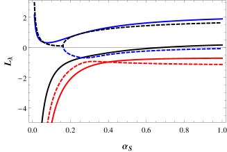
Figure 2: The different branch solutions $L_{\lambda}^{RG}(\alpha_{S},k)$ (solid curves) and $L_{\lambda}^{OPT}(\alpha_{S},k)$ (dashed curves), $k=1,2,3$, at $\delta^{3}$ (four-loop) order: left: $n_{f}=3$, right: $n_{f}=2$. Distinct branches appear to join within some $\alpha_{S}$ range where they actually become complex-conjugated, since only their real parts are plotted within this range.

In Fig. 2 we illustrate for $n_{f}=3$ (resp. left) and $n_{f}=2$ (resp. right) the different RG and OPT branches obtained at four loops, respectively as $L_{\lambda}^{RG}(\alpha_{S},k)$, $L_{\lambda}^{OPT}(\alpha_{S},k)$, where the number of solutions are at most $k=1,..3$ at four loops. The clearest situation is the one for $n_{f}=3$, where the two AF-matching RG and OPT branches (namely the two curves with the lowest $L_{\lambda}$ values for any $\alpha_{S}>0$ in Fig. 2) are real for any $\alpha_{S}>0$ and intersect at a unique value, that determines unambiguously the solution, compare last line in Table 2. Similar properties hold for all considered cases at lower orders. Next in Fig. 2 (right) for $n_{f}=2$, two of the OPT branches unconveniently become complex (conjugate)-valued within the range $0.25\lesssim\alpha_{S}\lesssim 0.33$ (so that their real parts shown here appear joined). Nevertheless one can still unambiguously select the correct AF-matching OPT branch, that is the one intersecting with the AF-matching RG branch, so that the correct solution is again unique.

V.2 Five-loop and six-loop results

Up to four loops, all the perturbative coefficients and RG quantities entering our evaluation have been known exactly for some time. Thanks to the recently calculated five-loop vacuum anomalous dimensionga05l , Eq.(62), and the very recent complete calculationmaier0919 of the four-loop nonlogarithmic coefficient $c_{44}(n_{f})$, given in Eq.(26), all the relevant perturbative coefficients needed at five loops are exactly available for the spectral density, Eq.(32). Thus we can extend our evaluation for the physically relevant $n_{f}=2,3$ values to five-loop order, correspondingly including up to five-loop contributions in the RG $\beta$ and $\gamma_{m}$ functions within the optimization, after performing consistently the $\delta$-expansion in Eq. (13) to order $\delta^{4}$. As mentioned above it is also useful to estimate the sensitivity of our results to the well-defined approximation Eq.(25) neglecting in $c_{44}$ the (subdominant) four-loop singlet contributions. Furthermore, higher-order coefficients are (partly) determinable solely from perturbative RG invariance, a feature that we can exploit to consider also (approximate) six-loop results (RGOPT order $\delta^{5}$). More precisely all the presently known five-loop RG coefficients, together with the complete four-loop coefficients, allow to determine exactly the six-loop coefficients $c_{6k}$, $0\leq k\leq 4$ of $\ln^{6-k}(m/\mu)$ of Eq.(16). While the single logarithmic term ($k=5$) would need the presently unknown six-loop vacuum energy anomalous dimension as well as the five-loop nonlogarithmic coefficient $c_{55}$. The explicit expressions of the $c_{6k}$ are given in Eq.(71) in Appendix. Consequently from Eq.(31) all the six-loop logarithmic terms, $\rho_{6k}L_{\lambda}^{6-k}$, $k=1,5$ of the spectral density in Eq. (32) are exactly predicted (see Eq.(72)), except for its last unknown nonlogarithmic coefficient. As we will examine below, the six-loop results, although being approximate, are quite important to assess a more reliable determination of the condensate, due to the occurence of rather unwelcome instabilities for the strictly five-loop results.

V.2.1 Five-loop and six-loop $n_{f}=2$ results

We examine now in some details our procedure and results for $n_{f}=2$, with quite similar features given more briefly below for $n_{f}=3$, except when important differences need to be mentioned. For $n_{f}=2$, at five loops we obtain one real solution that appears at first sight the closest to the lower (four-loop) results, namely: $L_{\tilde{\lambda}}=-0.5699,{\tilde{\alpha}_{S}}=0.5963$, which gives $\langle\bar{q}q\rangle^{1/3}_{RGI}\simeq-0.863\bar{\Lambda}_{2}$, obtained using the RG equation at five-loops. (Very close results are obtained if using instead the RG equation at four loops). Without further inquiries one would conclude from this result that the five-loops RGOPT produces an anomalously large shift of the condensate value, as compared with the seemingly well-stabilized three- and four-loop results $\sim-(0.78-0.77)$ in Table 1. A directly related issue is the anomalously large optimized coupling that corresponds to this solution, $\alpha_{S}\sim 0.6$, in contrast with the regularly decreasing coupling obtained at increasing orders up to four loops, in Tables 1, 2.
However, upon applying our general criteria to select the correct solutions, a more careful examination shows that this solution cannot be correct, since it is not sitting on the perturbative AF-matching branch, in contrast to what occurs systematically at lower orders. This feature can be checked rather easily by perturbatively expanding at first order the four different branch solutions for RG and OPT Eqs. respectively, that both give quartic equations in $L_{\lambda}\equiv\ln(\lambda/\mu)$ at five-loops (thus respectively giving $L_{\lambda}^{RG}(\alpha_{S},k)$, $L_{\lambda}^{OPT}(\alpha_{S},k)$ with $k=1,..4$), and examining which one(s) exhibit the perturbative AF-matching behavior, and whether the latter are matching the optimized $L_{\tilde{\lambda}},\tilde{\alpha}_{S}$ values obtained at the intersecting solution(s). Equivalently it can be seen more pictorially in Fig. 3, illustrating the different branches and (some of) their intersecting solutions (these branches are shown in a somewhat restricted but physically relevant range of $L_{\lambda}$ and $\alpha_{S}$): in contrast with the four-loop results in Fig. 2, the RG branches now also become complex, similarly to the OPT branches, within a rather important $\alpha_{S}$ range: $0.27\lesssim\alpha_{S}\lesssim 0.56$, and the only real intersection occuring at $\alpha_{S}\simeq 0.596,L_{\tilde{\lambda}}\simeq-0.57$ (visible near the top-right of Fig. 3) sits on RG and OPT branches that are not linked to the correct AF behavior.

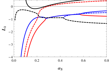
Figure 3: Some of the different RG (solid curves) and OPT (dashed curves) branches, respectively $L_{\lambda}^{RG}(\alpha_{S})$, $L_{\lambda}^{OPT}(\alpha_{S})$ at $\delta^{4}$ (five-loop) order for $n_{f}=2$. Distinct branches appear to join within some $\alpha_{S}$ range where they actually become complex conjugate, since only their real parts are plotted within this range.

Therefore, at five-loop order the RG and OPT AF-matching branch do not have a real-valued common intersection: a feature which somewhat complicates our investigation as compared with lower orders. This large perturbation, sufficiently destabilizing the regular trend observed at lower orders to suppress real AF-matching solutions, has two distinct, clearly identified origins. The first feature (but having a rather moderate impact on final results) is that the five-loop vacuum anomalous dimension coefficient ga05l is much larger relative to lower orders, moreover varying very much with $n_{f}$ (compare $\Gamma^{0}_{4}$ in Eq.(62) with $\Gamma^{0}_{3}$ in Eq.(61) in Appendix). (In contrast, as illustrated below, going from the four-loop to the five-loop $\beta$-function for the RG equation has a very modest impact, which can be traced to the moderate numerical changes of adding five-loop RG coefficients to $\beta(\alpha_{S})$, $\gamma_{m}(\alpha_{S})$ functions). Note that $\Gamma^{0}_{4}$ enters the five-loop condensate $L_{m}$ coefficient $c_{54}(n_{f})$, but it is not the sole contribution: the net effect from $\Gamma^{0}_{4}$ is typically that $|c_{54}(n_{f})/c_{50}(n_{f})|\sim 10$ roughly, which may be compared qualitatively with the similar four-loop quantities giving $|c_{43}/c_{40}|\sim 3$. But the second feature, that upon inspection happens to be the principal reason why the AF-matching solution is pushed into the complex domain, is that the discontinuities from Eq.(30) entail also a relatively large term $\sim\pi^{4}$, appearing for the first time at five-loop order in $\rho(\lambda,a_{s})$, within the nonlogarithmic coefficient. More precisely, it is the last term of Eq.(34), modifying the relevant original perturbative coefficient, $c_{54}(n_{f})$ in Eq. (16) by about $60\%$, while all other coefficients are more moderately affected by the discontinuity contributions. Simply ignoring this contribution would be clearly inconsistent, and we will examine below how to better circumvent those problems.
Note on Fig. 3 that the AF-matching RG and OPT branches have not disappeared but just became complex (conjugate) valued within a certain $\alpha_{S}$ range, rather unfortunately where the sought intersecting solution is expected. Indeed one can determine precisely the complex-conjugated solution that sits on the AF-matching branch: using the four-loop RG equation, we obtain: $L_{\tilde{\lambda}}\simeq-0.778\pm 0.303i,\tilde{\alpha}_{S}\simeq 0.358\pm 0.0537i$, that gives for the (RG invariant) condensate: $\simeq-(0.801\pm 0.0195i)\bar{\Lambda}(2)$ (see Table 3 for more details). Accordingly the correct AF-matching branch, although complex-valued in the relevant range, happens to give a corresponding condensate value with a small imaginary part, and with a real part in smoother continuity with the four-loop real solution. Also the corresponding (real part of the) optimal coupling $\tilde{\alpha}_{S}$ is more reasonably smaller than for the (wrong) naive real solution above. Very similar results are obtained if using rather the five-loop RG equation (see Table 3).

At this stage without further investigation one may just take the real part as the physically relevant result, and interpret the imaginary parts as a rough estimate of the theoretical uncertainties of the results (although this is presumably not the best possible prescription to estimate the intrinsic uncertainties). But given that the unwelcome occurence of nonreal solutions is only a consequence of solving exactly the RG and OPT polynomial equations in $L_{\lambda}$, and that it is seemingly not far from a real solution at five loops, one can more appropriately attempt to recover real solutions by a variant of the procedure. Accordingly a first possibility is simply to (perturbatively) approximate the sought optimized solutions at five loops. Alternatively another possibility is to proceed to next (six-loop) order: at least this is possible in the approximation of neglecting the nonlogarithmic six-loop coefficient, being the only contribution not presently derivable from already known lower order results (as explained above at the beginning of SubSec. V.2). Let us examine in turn those two possibilities.

V.2.2 Perturbatively truncated five-loop RG solutions

At five loops, instead of solving exactly the relevant RG and/or OPT optimization Eqs.(12), (14), one can consider more perturbative approximations, as long as those remain consistent with the original perturbative order considered. Indeed the RG Eq.(12) generates terms of formally higher order than five loops: more precisely it is easy to see that at five loops Eq.(12) acting on the five-loop ($\alpha_{S}^{4}$) spectral density Eq.(32) involves up to $\alpha_{S}^{9}$ terms, due to the highest five-loop RG contributions $\propto b_{4}\alpha_{S}^{6}$, $\gamma_{4}\alpha_{S}^{5}$ respectively. But $b_{4}$, $\gamma_{4}$ appear first at order $\alpha_{S}^{5}$, $\alpha_{S}^{4}$ respectively. Accordingly a presumably sensible procedure is to truncatergopt_Lam the RG equation, suppressing higher-order terms in $\alpha_{S}$ until possibly recovering a real common RG and OPT solution. At the same time if suppressing too many higher-order terms one loses the consistency with the RG content required at a given (here four- or five-loop) order. A similar reasoning shows that the next order six-loop RG coefficients, $b_{5},\gamma_{5}$ (presently not known), would enter first respectively the $\alpha_{S}^{6}$, $\alpha_{S}^{5}$ coefficients of the RG equation.
Therefore it appears sensible to truncate any $\alpha_{S}^{k}$, $k\geq 6$ in the result of Eq. (12), that would be anyway affected by presently unknown higher orders. Further truncating the $\alpha_{S}^{5}$ term implies, however, losing any dependence from the five-loop $b_{4}$ (while it still involves the five-loop $\gamma_{4}$ one). Accordingly we found instructive to consider the effects of successive truncations, progressively suppressing the highest $\alpha_{S}^{9}$ down to $\alpha_{S}^{6}$ (or even possibly $\alpha_{S}^{5}$) terms and comparing. This is done below, with all results compiled in Table 3 obtained by optimizing the spectral density $\rho(\lambda,\alpha_{S})$ and keeping only the AF-matching branch solution (unique at a given order).

Table 3: $n_{f}=2$ results at RGOPT $\delta^{4}$ (five-loops) and partial $\delta^{5}$ (six-loops) for the (RG invariant) condensate $\langle\bar{q}q\rangle^{1/3}_{RGI}/\bar{\Lambda}_{2}$ and the corresponding optimal values of the spectral parameter $\tilde{\lambda}$, coupling $\tilde{\alpha}_{S}$, and scale $\tilde{\mu}$, from optimizing $\rho(\lambda,\alpha_{S})$ with Eqs. (14), (12). We compare the results of (perturbatively consistent) successive RG equation truncations. $\bar{\Lambda}_{2}$ is normalized by Eq. (37) when the four-loop RG equation is used or by its five-loop extension when the five-loop RG equation is used.

RGOPT[$\rho(\lambda,\alpha_{S})$]
$\delta^{k}$, RG order	$\ln\frac{\tilde{\lambda}}{\mu}$	$\tilde{\alpha}_{S}$	$\frac{-\langle\bar{q}q\rangle^{1/3}_{RGI}}{\bar{\Lambda}_{2}}$	$\frac{\mu}{\bar{\Lambda}_{2}}$
$\delta^{4}$, RG 4-loop (full)	$-0.77785\pm 0.30316i$	$0.35785\pm 0.053706i$	$0.80084\pm 0.019516i$	$3.6418$
$\delta^{4}$, RG 5-loop (full)	$-0.78815\pm 0.31499i$	$0.35181\pm 0.0501i$	$0.80104\pm 0.019553i$	$3.7403$
$\delta^{4}$, RG 5-loop ($\alpha_{S}^{\bcancel{k\geq 9}}$)	$-0.80175\pm 0.3081i$	$0.35384\pm 0.043583i$	$0.80101\pm 0.019379i$	$3.7596$
$\delta^{4}$, RG 4-loop ($\alpha_{S}^{\bcancel{k\geq 8}}$)	$-0.81664\pm 0.29248i$	$0.35958\pm 0.036002i$	$0.80033\pm 0.018530i$	$3.7292$
$\delta^{4}$, RG 5-loop ($\alpha_{S}^{\bcancel{k\geq 8}}$)	$-0.8151\pm 0.28951i$	$0.36097\pm 0.036464i$	$0.8009\pm 0.018641i$	$3.7094$
$\delta^{4}$, RG 4-loop ($\alpha_{S}^{\bcancel{k\geq 7}}$)	$-0.83759\pm 0.25140i$	$0.37539\pm 0.024696i$	$0.80048\pm 0.015453i$	$3.5816$
$\delta^{4}$, RG 5-loop ($\alpha_{S}^{\bcancel{k\geq 7}}$)	$-0.83618\pm 0.250i$	$0.37603\pm 0.025177i$	$0.80121\pm 0.01559i$	$3.5728$
$\delta^{4}$, RG 4-loop ($\alpha_{S}^{\bcancel{k\geq 6}}$)	$-0.93852\pm 0.17354i$	$0.40216\pm 0.01192i$	$0.79914\pm 0.0004024i$	$3.3298$
$\delta^{4}$, RG 5-loop ($\alpha_{S}^{\bcancel{k\geq 6}}$)	$-0.93840\pm 0.17332i$	$0.40223\pm 0.011871i$	$0.79994\pm 0.0004919i$	$3.3292$
$\delta^{5}$, RG 5-loop (full)	$-1.0846$	$0.32689$	$0.77133$	$4.3737$
$\delta^{5}$, RG 5-loop ($\alpha_{S}^{\bcancel{k\geq 6}}$)	$-1.1422$	$0.33778$	$0.77260$	$4.1671$

From the $n_{f}=2$ results of Table 3, at five loops it appears not that easy to recover real solutions: upon truncating terms progressively starting from highest order ones, the results do not change much at first, although there is a slow but clear decrease of the corresponding imaginary parts. Also, despite the not small $Im[L_{\tilde{\lambda}}]$ values, the resulting condensate has much smaller imaginary parts, and real parts remain very stable, differing relatively only by ${\cal O}(10^{-3})$ for the different truncations. Similarly, for all cases there are tiny differences between the results using the four-loop or five-loop RG equation. The $\tilde{\alpha}_{S}$ value are also more reasonably perturbative, and close to the real four-loop results of Table 1. Truncating maximally the RG equation (namely by all terms $\alpha_{S}^{k\geq 6}$, but that still involves all the five-loop RG coefficients), the correct (AF-matching) solution has a tiny imaginary part, so that its real part may be considered reliable, giving $\langle\bar{q}q\rangle^{1/3}_{RGI}\simeq-(0.800\pm 0.0005i)\bar{\Lambda}_{2}$. Note that if further truncating the RG equation, one not only loses the consistent RG content at five-loop order, but the corresponding RG equation no longer gives any AF-matching branch.

V.2.3 Approximate (partial) six-loop RGOPT

As sketched above, the second alternative is to proceed at next (six-loop) order of Eq.(32), with the $\ln^{6-k}(\lambda)$ coefficients given explicitly in Appendix (see Eqs.(71), (72)). The motivation, apart simply from the fact that most of the six-loop coefficients are readily exploitable from RG properties, is that the discontinuities (30) entail additional contributions $\propto\pi^{4}$ (see the last terms in Eq.(31)), that tend to partially balance the instability triggered by $\pi^{4}$ discontinuity terms appearing first at five-loop order. At this point it is worth remarking that such features are generically expected from Eq.(30): typically in rgoqq1 we have calculated the spectral density for the Gross-Neveu (GN) $O(N)$ model GN in the large-$N$ limit, to very high perturbative orders, that exhibits a clear pattern: the RGOPT solutions at increasing orders converge slowly towards the exact result (known for the GN model), those solutions being destabilized each time novel $\pi^{2k}$ contributions appear first, at increasing orders . However, if keeping only fixed $\pi^{2k}$ terms (namely discarding $\pi^{2k+2}$, etc, terms appearing at higher orders), remarkably at sufficiently high fixed order all the $\pi^{2k}$ terms cancel, and the exact GN spectral density is obtained rgoqq1 .

For the QCD spectral density such exact cancellations are not expected, moreover obviously we are quite limited in trying to reach still higher orders. But inspired from these properties it is worth comparing two available successive orders (five and six loops), that actually rely on the same five-loop RG content, since as we recall, five-loop RG properties predict most of the six-loop coefficients of $\rho(\lambda)$ (all except the nonlogarithmic one, $\rho_{66}$ in Eq.(32). Accordingly one should keep in mind that it remains an approximation to the complete six-loop results, since $\rho_{66}$ involves the presently unknown six-loop vacuum anomalous dimension and the five-loop nonlogarithmic coefficient $c_{55}$. Therefore we simply set $\rho_{66}$ to zero in our numerics (neglecting also consistently the other nonlogarithmic contributions, generated at six loops from the discontinuities (31). We will argue below that this approximation should moderately deviate from the complete six-loop results.

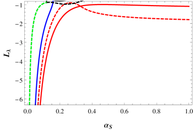
Figure 4: Some of the relevant RG (solid curves) and OPT (dashed curves) branches, respectively $L_{\lambda}^{RG}(\alpha_{S})$, $L_{\lambda}^{OPT}(\alpha_{S})$ at $\delta^{5}$ (6-loop) order for $n_{f}=2$.

For $n_{f}=2$ the corresponding partial six-loop RGOPT results are given in the last two lines of Table 3, also considering the (maximal) RG consistent truncation. As one can see a real solution is recovered at six loops, moreover the two AF-matching RG and OPT branches remain real for all the physically relevant $\alpha_{S}$ range, and their intersection occur for a substantially smaller $\tilde{\alpha}_{S}$ value as compared to five loops. This is illustrated also in Fig. 4, zooming on the RG and OPT branches in the relevant range of $L_{\lambda},\alpha_{S}$, which looks qualitatively more similar to the four-loop $n_{f}=3$ case. It is striking that the resulting condensate value is much closer to the four-loop results, that is not a numerical accident but is more essentially the effect of partially balancing at six loops the instability from the large $\pi^{4}$ terms occuring first at five loops.

V.2.4 Summary of $n_{f}=2$ results

As a tentative summary of the previous $n_{f}=2$ investigation:

• At five loops, the impact of both large five-loop vacuum energy anomalous dimensions and (more importantly) the first occurence of $\pi^{4}$ terms from (30), are strong enough to destabilize the regular features observed at lower orders up to four loops. Consequently one fails to obtain a strictly real AF-matching solution. Yet the five-loop results from successive truncations of unmandatory higher order terms in the RG equation are very consistent, reflecting a good stability. Also the imaginary parts are small enough (especially for the maximal truncation of $\alpha_{S}^{k\geq 6}$, see Table 3) and can be included within the theoretical uncertainties.

• Next, going to six loops restores a real unique AF-matching solution, that results from a partial balance of the destabilizing $\pi^{4}$ terms. This solution has very regular properties and happens to be very close to the four-loop results.

These properties are more generically confirmed from comparison with the other relevant values $n_{f}=3$, or $n_{f}=0$, as illustrated next.

V.3 Five- and six-loop $n_{f}=3$ results

Table 4: $n_{f}=3$ results at five- and six-loops: same captions as in Table 3.

RGOPT[$\rho(\lambda,\alpha_{S})$]
$\delta^{k}$, RG order	$\ln\frac{\tilde{\lambda}}{\mu}$	$\tilde{\alpha}_{S}$	$\frac{-\langle\bar{q}q\rangle^{1/3}_{RGI}}{\bar{\Lambda}_{3}}$	$\frac{\mu}{\bar{\Lambda}_{3}}$
$\delta^{4}$, RG 4-loop (full)	$-0.92148\pm 0.29624i$	$0.36925\pm 0.051547i$	$0.76927\pm 0.016561i$	$3.9124$
$\delta^{4}$, RG 5-loop (full)	$-0.93013\pm 0.3038i$	$0.36465\pm 0.04859i$	$0.76838\pm 0.016134i$	$3.9911$
$\delta^{4}$, RG 4-loop ($\alpha_{S}^{\bcancel{k\geq 6}}$)	$-1.064\pm 0.13845i$	$0.42391\pm 0.012618i$	$0.77089\pm 0.0024578i$	$3.4384$
$\delta^{4}$, RG 5-loop ($\alpha_{S}^{\bcancel{k\geq 6}}$)	$-1.0639\pm 0.13833i$	$0.42394\pm 0.012593i$	$0.76975\pm 0.0023702i$	$3.4297$
$\delta^{5}$, RG 5-loop (full)	$-1.2340$	$0.33863$	$0.74042$	$4.6923$
$\delta^{5}$, RG 5-loop ($\alpha_{S}^{\bcancel{k\geq 6}}$)	$-1.2618$	$0.3449$	$0.74076$	$4.5578$

For $n_{f}=3$ at five loops, very similarly to $n_{f}=2$ there is one real RGOPT solution appearing at first the closest to the four-loop real results, using the RG equation at five loops: $L_{\tilde{\lambda}}\simeq-0.693411$, $\tilde{\alpha}_{S}\simeq 0.598$. This gives for the RG invariant condensate: $\simeq-0.813\bar{\Lambda}_{3}$, thus a large shift from four-loop results of Table 2. But again upon examining the AF branches these do not match with this real solution, and the correct AF-matching but complex-valued branch gives a more reasonable result, with small imaginary parts and real part closer to four-loop real results (see Table 4).
Similarly to $n_{f}=2$ we have performed a systematic analysis of all possible RG consistent truncations. We illustrate in Table 4 the more relevant results, omitting intermediate case details. Overall the behavior is much similar to $n_{f}=2$: at five loops one fails to recover strictly real AF-matching solutions, but the maximal truncation (discarding $\alpha_{S}^{k\geq 6}$, not loosing the five-loop RG content) gives very small imaginary parts, and we will take the real part and add appropriate uncertainties in our final estimate.
Next, similarly to the $n_{f}=2$ results, at six-loop order one recovers a real AF-matching solution given in the last two lines in Table 4, with very regular properties and close to the four-loop results of Table 2.

V.4 Impact of approximated five-loop contributions

We now consider the approximation, defined in subsection IV.2 and relevant for $n_{f}=2,3$, of using for the four-loop nonlogarithmic coefficient $c_{44}$ our expression in Eq. (25) derived from the related nonsinglet four-loop scalar two-point correlatorPiSns4l . We recall that at the level of the optimized spectral density, this affects results only via the five-loop single logarithmic coefficient $c_{54}$. Since the previous results in subSec.V.2 including the very recently determinedmaier0919 exact $c_{44}$ coefficient Eq. (26) are accordingly more complete, we will not include the variations resulting from this approximation within our uncertainty estimates. Nevertheless, given that the more exact five-loop results above are somewhat prevented by instabilities from producing real solutions, it is instructive to study their sensitivity upon such a well-defined approximation. The corresponding results are shown in Table 5 for $n_{f}=2$ and $n_{f}=3$ at five- and six-loops.

Very similarly to the results obtained with the full $c_{44}$, at five loops the RGOPT gives nonreal AF-matching solutions, but with small imaginary parts. Accordingly in Table 5 the results are not too different from the ones from using the exact $c_{44}$ in Tables 3, 4, except that the imaginary parts are somewhat smaller. For $n_{f}=3$, real AF-matching solutions are recovered upon maximal truncations consistent with RG at five loops. At six loops real AF-matching solutions are also recovered, and these differ from the ones with exact $c_{44}$ in Tables 3, 4 by about $\sim 1\%$ ($\sim 2\%$) lower in $\bar{\Lambda}$ units for $n_{f}=2$ ($n_{f}=3$) respectively. All these features are consistent with the fact that the loss of real solution at five loops is essentially due to the occurence of relatively large $\pi^{4}$ terms, while the $\sim 4\%$ ($\sim 7\%$) for $n_{f}=2$ ($n_{f}=3$) decrease in the approximated $c_{44}$ Eq.(25), as compared with the complete one Eq.(26), has a more moderate impact.
We conclude that the approximation neglecting the four-loop singlet contributions within $c_{44}$ produces a change in the final condensate magnitude $|\langle\bar{q}q\rangle|^{1/3}$ that is about $\sim 1\%(2\%)$ smaller in magnitude respectively for $n_{f}=2$ ($n_{f}=3$), which again reflects a good overall stability.

Table 5: $n_{f}=2$ and $n_{f}=3$ results at five and six loops using the approximate $c^{IS}_{44}$ coefficient from Eq.(25). Same captions as in Tables 4.

RGOPT[$\rho(\lambda,\alpha_{S})$]
$\delta^{k}$, RG order	$\ln\frac{\tilde{\lambda}}{\mu}$	$\tilde{\alpha}_{S}$	$\frac{-\langle\bar{q}q\rangle^{1/3}_{RGI}}{\bar{\Lambda}_{2}}$	$\frac{\mu}{\bar{\Lambda}_{2}}$
$n_{f}=2$:
$\delta^{4}$, RG 4-loop (full)	$-0.71996\pm 0.23156i$	$0.37549\pm 0.05979i$	$0.79341\pm 0.0099350i$	$3.4177$
$\delta^{4}$, RG 5-loop (full)	$-0.74047\pm 0.24939i$	$0.36580\pm 0.053884i$	$0.79353\pm 0.0098374i$	$3.5523$
$\delta^{4}$, RG 4-loop ($\alpha_{S}^{\bcancel{k\geq 6}}$)	$-0.92679\pm 0.10146i$	$0.39942\pm 0.0074906i$	$0.79090\pm 0.0015884i$	$3.3590$
$\delta^{4}$, RG 5-loop ($\alpha_{S}^{\bcancel{k\geq 6}}$)	$-0.926667\pm 0.10103i$	$0.39949\pm 0.0074377i$	$0.79166\pm 0.0016397i$	$3.3583$
$\delta^{5}$, RG 5-loop (full)	$-1.15411$	$0.32270$	$0.75896$	$4.4605$
$n_{f}=3$:	$\ln\frac{\tilde{\lambda}}{\mu}$	$\tilde{\alpha}_{S}$	$\frac{-\langle\bar{q}q\rangle^{1/3}_{RGI}}{\bar{\Lambda}_{3}}$	$\frac{\mu}{\bar{\Lambda}_{3}}$
$\delta^{4}$, RG 4-loop (full)	$-0.77002\pm 0.19327i$	$0.40513\pm 0.082108i$	$0.75375\pm 0.0019729i$	$3.3255$
$\delta^{4}$, RG 5-loop (full)	$-0.79824\pm 0.18251i$	$0.40213\pm 0.067656i$	$0.75291\pm 0.00097752i$	$3.4381$
$\delta^{4}$, RG 4-loop ($\alpha_{S}^{\bcancel{k\geq 6}}$)	$-1.1570$	$0.42880$	$0.76070$	$3.3996$
$\delta^{4}$, RG 5-loop ($\alpha_{S}^{\bcancel{k\geq 6}}$)	$-1.1572$	$0.42885$	$0.75957$	$3.3905$
$\delta^{5}$, RG 5-loop (full)	$-1.3589$	$0.33097$	$0.71983$	$4.8713$

V.5 The condensate in the quenched approximation

One can also easily extend our calculations formally for $n_{f}=0$: actually a quark of mass $m$, setting the overall scale in Eq.(16), ’dressed’ at higher orders by pure gauge interactions, is still understood in this case, and the perturbative removal of the quarks entering at three loops in Fig.1 and higher orders may be viewed as a perturbative analog of the ’quenched’ approximation, which has its own theoretical interest, and can be compared with lattice simulations as we will examine. Specializing our calculations to the quenched approximation from the known exact $n_{f}$ dependence in all relevant perturbative and RG coefficients, one simply takes $n_{f}=0$ everywhere consistently. Proceeding as previously described, from the first NLO (two-loop) nontrivial order up to five loops, gives the results in Table 6.

Table 6: $n_{f}=0$ (quenched approximation) results up to five loops: same captions as Table 1.

$\delta^{k}$ order	$\ln\frac{\tilde{\lambda}}{\mu}$	$\tilde{\alpha}_{S}$	$\frac{-\langle\bar{q}q\rangle^{1/3}_{RGI}}{\bar{\Lambda}_{0}}$	$\frac{\tilde{\mu}}{\bar{\Lambda}_{0}}$
$\delta$, RG 1-loop	$-\frac{179}{1452}$	$\frac{11\pi}{40}\simeq 0.86394$	$1.0072$	$1.9370$
$\delta$, RG 2-loop	$-0.27548$	$0.49747$	$0.9122$	$2.4945$
$\delta^{2}$, RG 2-loop	$-0.54201$	$0.47091$	$0.85679$	$2.5795$
$\delta^{2}$, RG 3-loop	$-0.54434$	$0.41691$	$0.83522$	$2.8224$
$\delta^{3}$, RG 3-loop	$-0.63438$	$0.39314$	$0.83741$	$2.9713$
$\delta^{3}$, RG 4-loop	$-0.60347$	$0.38002$	$0.83508$	$3.0687$
$\delta^{4}$, RG 4-loop	$-0.54077$	$0.39241$	$0.85253$	$2.9764$
$\delta^{4}$, RG 5-loop	$-0.45296$	$0.42275$	$0.86069$	$2.8045$

The solutions in Table 6 for the quenched case, up to five-loop order included, are all located on the real AF-matching branch (which is unique at a given order), although when using five-loop RG in the very last line, the solution is located very close to the border of non-AF-matching branches. We observe that the condensate magnitude $|\langle\bar{q}q\rangle|^{1/3}$ is driven to about $\sim 2.5\%$ higher values when going from four to five loops, as similarly observed above for $n_{f}=2,3$ in Tables 3, 4. As above mentioned this is essentially traced to the instability from the first occurence of $\pi^{4}$ discontinuity term at five loops.
Although in this quenched case one obtains at five loops a real solution upon using the complete RG, it is also instructive to examine the trend obtained from successive RG truncations, or alternatively when performing the calculation at six loops, giving the results in Table 7.

Table 7: $n_{f}=0$ results at five and sixloops: same captions as in Tables 3.

RGOPT[$\rho(\lambda,\alpha_{S})$]
$\delta^{k}$, RG order	$\ln\frac{\tilde{\lambda}}{\mu}$	$\tilde{\alpha}_{S}$	$\frac{-\langle\bar{q}q\rangle^{1/3}_{RGI}}{\bar{\Lambda}_{0}}$	$\frac{\mu}{\bar{\Lambda}_{0}}$
$\delta^{4}$, RG 4-loop (full)	$-0.54077$	$0.39241$	$0.85253$	$2.9764$
$\delta^{4}$, RG 5-loop (full)	$-0.45296$	$0.42275$	$0.86069$	$2.8045$
$\delta^{4}$, RG 4-loop ($\alpha_{S}^{\bcancel{k\geq 6}}$)	$-0.70122+0.11373i$	$0.36891-0.0031072i$	$0.84724+0.00030466i$	$3.1610$
$\delta^{4}$, RG 5-loop ($\alpha_{S}^{\bcancel{k\geq 6}}$)	$-0.70089+0.11265i$	$0.36906-0.0030291i$	$0.85101+0.00019590i$	$3.170$
$\delta^{5}$, RG 5-loop (full)	$-0.90052$	$0.30873$	$0.82242$	$3.912$
$\delta^{5}$, RG 5-loop ($\alpha_{S}^{\bcancel{k\geq 6}}$)	$-0.97183$	$0.31740$	$0.82383$	$3.772$

As one can see here it is the effect of RG truncation that pushes the AF-matching solution to (slightly) nonreal values. Comparing these RG-truncated results from Table 7, which have negligible imaginary parts, with the corresponding real solutions using the complete RG in Table 6, gives a useful estimate of the impact of such RG-consistent truncations. Concerning the six-loop results, very similarly to the $n_{f}=2$ and $n_{f}=3$ cases they are real and very regular, and again much closer to the four-loop results in Table 6.

Finally for completeness we have also considered the $n_{f}=1$ case: although it is not very relevant physically, it can be viewed at least as a further consistency crosscheck of our results. We have explored variants similarly to other $n_{f}$ values above but simply summarize here the main results. At four-loop order one obtains the unique real solution:

$$\langle\bar{q}q\rangle^{1/3}_{RGI}(n_{f}=1,\mbox{4-loop})=-0.8039\bar{\Lambda}_{1}$$ (39)

which appears very close to the ’average’ of $n_{f}=0$ and $n_{f}=2$ four-loop results. At five-loops, using four- or five-loop RG, the real solution is no longer on the AF-matching branch, similarly to the $n_{f}=2,3$ cases. The unique AF-matching solution obtained from truncating $\alpha_{S}^{k\geq 6}$ in the RG equation gives:

$$\langle\bar{q}q\rangle^{1/3}_{RGI}(n_{f}=1,\mbox{truncated RG 5-loop})=-(0.8271\pm 0.0007\,i)\bar{\Lambda}_{1}$$ (40)

Finally at six-loops a real solution is recovered, giving

$$\langle\bar{q}q\rangle^{1/3}_{RGI}(n_{f}=1,\mbox{RG five-loop})=-0.7984\bar{\Lambda}_{1}.$$ (41)

Similarly to $n_{f}=0,2,3$ cases, once more the five-loop results produce a substantial $\sim 2.8\%$ increase of the condensate as compared to four-loops results, while the six-loop results are very close to the latter.

V.6 Evaluating theoretical uncertainties

Comparing the different above results from $n_{f}=0$ to $n_{f}=3$, it is tempting to consider the manifestly more stable results obtained at four loops and six loops as a likely better approximation than the more sensibly shifted five-loop results. Note indeed that if discarding the latter, the combined 4-loop and 6-loop results would provide a seemingly very accurate determination. But since the six-loop results are only partial, we more conservatively combine all those results within our estimate of uncertainties. More precisely we take the average between the four-, five- and six-loop results as our central values and their differences as our theoretical uncertainties (taking at five loops the real parts of the results having the smallest imaginary parts, that are consequently more reliable). Then we estimate the uncertainties linearly from the complete range spanned by maximal and minimal values.

For $n_{f}=0$, for which real solutions occur at all RGOPT successive orders considered, we obtain

$$\langle\bar{q}q\rangle^{1/3}_{RGI}(n_{f}=0)\simeq-(0.840_{-0.016}^{+0.020})\bar{\Lambda}_{0},$$ (42)

where we give only a three digits accuracy given the uncertainties.

For $n_{f}=2$, proceeding similarly we obtain

$$\langle\bar{q}q\rangle^{1/3}_{RGI}(n_{f}=2)\simeq-(0.781_{-0.009}^{+0.019})\bar{\Lambda}_{2}.$$ (43)

And finally for $n_{f}=3$:

$$\langle\bar{q}q\rangle^{1/3}_{RGI}(n_{f}=3)\simeq-(0.751_{-.010}^{+0.019})\bar{\Lambda}_{3}.$$ (44)

Eqs (42),(43), (44) constitute our primary results, as these do not depend on any extra theoretical or experimental input besides the basic perturbative content used in the calculation and the RGOPT method. Now, to make contact with other independent determinations of the quark condensate, often conventionally given at the standard scale $\mu\simeq 2$ GeV for reference, one needs to perform a (perturbative) renormalization scale evolution. One should keep in mind that, in contrast with the above results, such RG evolution unavoidably also entails $\alpha_{s}$ (and other related) uncertainties.

VI $\langle\bar{q}q\rangle(\mu=2\,\rm GeV)$ and comparison with other determinations

To evolve perturbatively the condensate from our results above, the simplest procedure is to take the values obtained for the scale-invariant condensate (38), within uncertainties, Eqs.(42)-(44) and extract from these the condensate at another chosen (perturbative) scale $\mu^{\prime}$, using again (38) at five-loop order, now taking $g\equiv 4\pi\alpha_{S}(\mu^{\prime})$, after evolving $\alpha_{S}(\mu)$ at five-loop order of Eq.(37) towards the conventional scale $\mu^{\prime}=2$ GeV. The overall reliability of this (perturbative) evolution is to be assessed on the ground that the primary RGOPT results above at four-, five- and six-loops are obtained at reasonably perturbative optimized scale values ($3.3\Lambda_{\overline{MS}}\lesssim\tilde{\mu}\lesssim 4.8\Lambda_{\overline{MS}}$ (compare Tables 1-4). It is more appropriate to separate the discussion below for different $n_{f}$ values, since those do not have all the same reliability status (also when comparing our results with other independent determinations of the condensate) as we discuss next. We consider successively $n_{f}=3$, $n_{f}=2$, and $n_{f}=0$ (quenched approximation).

VI.1 $n_{f}=3$

For $n_{f}=3$, one can use very reliable $\alpha_{S}$ determinations in the perturbative range. We also account properly for the charm quark mass threshold effectsmatching4l on $\alpha_{S}(\mu\sim m_{c})$. From the most recent world average $\alpha_{S}(m_{Z})$ value PDG :

$$\alpha_{S}(m_{Z})=0.1179\pm 0.0010,$$ (45)

we obtain in a first stage, accounting for threshold effects at $\mu\sim m_{b}$ and $\mu\sim m_{c}$ :

$$\bar{\Lambda}(n_{f}=3)=(331\pm 16)\,\mbox{MeV}$$ (46)

and

$$\alpha_{S}(2\,\mbox{GeV})=0.3007\pm 0.008.\;\;$$ (47)

Then using Eq. (38) applied to Eq.(44) leads to

$$\langle\bar{q}q\rangle^{1/3}_{n_{f}=3}(2\,{\rm GeV})=-(0.826_{-.011}^{+.021})\bar{\Lambda}_{3}\;.$$ (48)

Thus combining Eq.(46) with (48) leads to

$$\langle\bar{q}q\rangle^{1/3}_{n_{f}=3}(2\,{\rm GeV},\rm\bar{\Lambda}^{wa}_{3})\simeq-(273^{+7}_{-4}\pm 13)\,{\rm MeV}\,$$ (49)

where the first error is our rather conservative theoretical RGOPT uncertainty from Eq.(48) and the second one is from $\bar{\Lambda}(3)$ uncertainty. (Since these two uncertainties have very different origin we do not combine them). It is worth remarking at this point that Eq. (48) is only slightly shifted with respect to our previous (average of three- and four-loop RGOPT) result rgoqq1 , while the central value and uncertainties in Eq.(49) (compare Eq.(6.6) of rgoqq1 ) are principally affected by the slight decrease of the most recent $\alpha_{S}$ world average with substantial increase of uncertainties (see PDG for detailed explanations on these features).
To compare with other independent determinations, first the most precise $n_{f}=3$ lattice determination we are aware of, in the chiral limit, is $\langle\bar{q}q\rangle^{1/3}_{n_{f}=3}(2\rm GeV)=-(245\pm 5\pm 8)$ MeV Lattqqn3 . Our results are thus marginally compatible with the latter, within uncertainties of both results. Note, however, that various recent lattice results vary in a wider range for $n_{f}=3$, as compiled from LattFLAG19 : from $214\pm 6\pm 24$ Lattqqn3_low to $290\pm 15$ Lattqqn3_high . This is largely due to the still difficult required extrapolation of lattice results to the chiral limit, which for the $SU(3)$ case is affected by large uncertainties. A recent very precise $n_{f}=3$ lattice calculationLattqqn3_corr , using time-moments of heavy-strange pseudoscalar correlator, has obtained $\langle\bar{s}s\rangle^{1/3}(\mbox{2 GeV})\sim-(296\pm 11)$ MeV. Since it is not in the chiral limit, it should not be directly compared with our result, given the large strange quark mass involved. Indeed as our $n_{f}=3$ results are based on a relatively accurate RGOPT determination (44), and (49) obtained from a reliable $\bar{\Lambda}(3)$ world average, they appear useful independent determinations since being in the strict chiral limit, thus relevant to possibly assess the actual impact from explicit chiral symmetry breaking by the strange quark mass, by comparison with other determinations that include the latter, like Lattqqn3_corr .

VI.2 $n_{f}=2$

For $n_{f}=2$, one cannot directly link our results to the true phenomenological perturbative range values of $\alpha_{S}$ as above. Nevertheless, given that the (optimized) coupling values obtained in Table 1, 3 are reasonably perturbative, we can consider a perturbative (five-loop) RG evolution (consistently performed in a simplified QCD picture where the strange and heavier quarks are all infinitely massive, i.e. ‘integrated out’). To give a final (numerical) determination of the condensate, we need a value for $\bar{\Lambda}(n_{f}=2)$. To our knowledge there are not so many nonperturbative results for $\bar{\Lambda}(2)$ (as compared with the numerous studies for $n_{f}=3$), and those results mostly originate from lattice calculations. We therefore rely on a lattice determinationLam2_latt_ALPHA (that best fulfill the reliability criteria of the review LattFLAG19 ), obtained from the Schrödinger functional method:

$$\bar{\Lambda}(n_{f}=2)=(310\pm 20)\,\mbox{MeV}.$$ (50)

One should keep in mind, however, that somewhat larger uncertainties are obtained if taking more conservatively all presently available lattice resultsLam2_latt_ALPHA ; Lam2_latt_other , as compiled in LattFLAG19  . After RG evolution up to 2 GeV we obtain accordingly from Eq.(43):

$$\langle\bar{q}q\rangle^{1/3}_{n_{f}=2}(2\,{\rm GeV})=-(0.863_{-.010}^{+.021})\bar{\Lambda}_{2}.$$ (51)

(Notice that this strictly $n_{f}=2$ result, thus with the strange and heavier quarks integrated out, correspondingly has $\alpha_{S}(\mu)$ values not consistent with the phenomenological values of Eq.(47): instead we find $\alpha_{S}^{n_{f}=2}(\mbox{2 GeV})\simeq 0.262\pm.008$). Combining (51) with Eq. (50) leads to 

$$\langle\bar{q}q\rangle^{1/3}_{n_{f}=2}(2{\rm GeV},\rm\bar{\Lambda}_{2})\simeq-(267^{+7}_{-4}\pm 18)\,{\rm MeV}\,,$$ (52)

where again the first error range is our RGOPT uncertainty from Eq.(51) while the second one is from the $\bar{\Lambda}(2)$ uncertainty. Since lattice uncertainties are mostly statistical and systematic, while ours are theoretical, it is not obvious to combine these in a sensible manner and we keep more conservatively separate uncertainties.
To compare our result (52) with other recent determinations, first the presumably most precise $n_{f}=2$ lattice determination to date is also from the spectral density SDlatt_recent : $\langle\bar{q}q\rangle^{1/3}_{n_{f}=2}(\mu=2{\rm GeV})=-(261\pm 6\pm 8)$, where the first error is statistical and the second is systematic. Our results are thus very compatible within uncertainties. Note, however, that the above quoted lattice value SDlatt_recent was obtained by fixing the scale with the kaon decay constant $F_{K}$, determined in the quenched approximation. Overall, recent $n_{f}=2$ lattice determinations of the condensate in the chiral limit from several independent methods are much more precise than those for $n_{f}=3$. We quote the estimate recently performed in LattFLAG19 , by combining results from SDlatt_recent ; qqlatt_n2 : $|\langle\bar{q}q\rangle|^{1/3}_{n_{f}=2}=-(266\pm 10)$ MeV, where the uncertainties include both systematic and statistical ones.

One may also compare with recent results from spectral sum rules qqSRlast : $\langle\bar{u}u\rangle^{1/3}(\equiv\langle\bar{d}d\rangle^{1/3})(\mbox{2 GeV})\simeq-(276\pm 7)$ MeV. But keeping in mind that the latter sum rules actually determine precisely the current quark masses, so that the $\langle\bar{u}u\rangle$ value is indirectly extracted from using the GMOR relation (1). Accordingly the comparison is not strictly for the chiral limit. In this context, even though the overall reliability of $\bar{\Lambda}(2)$ is not yet at the level of $\bar{\Lambda}(3)$, the results (43) and (52) constitute reasonably accurate independent determinations in the chiral limit. Indeed, given that the present $n_{f}=2$ lattice results for the condensate are quite accurate, it is tempting alternatively to combine the latter with our firmer result Eq.(43), in order to rather determine a new independent estimate of $\bar{\Lambda}(2)$: taking the above quoted estimate of the condensate given by LattFLAG19 , this gives

$$\bar{\Lambda}(n_{f}=2)=(308^{+4}_{-6}\pm 12)\mbox{MeV}.$$ (53)

VI.3 $n_{f}=0$ (quenched approximation)

Finally for completeness we also give results for the quenched approximation ($n_{f}=0$). In this case we evolve $\alpha_{S}(\mu)$ and use Eq. (38) at five loops but in the appropriate $n_{f}=0$ approximation. As previously we need $\bar{\Lambda}(n_{f}=0)$, available from various different approaches with lattice simulations. We rely on the average performed in LattFLAG19 , combining different precise lattice resultslattLam0 :

$$\bar{\Lambda}(n_{f}=0)=(257\pm 7)\,\mbox{MeV}.$$ (54)

As stressed in LattFLAG19 , it is worth noting that this value is obtained by using the same value as for $n_{f}=2$ and $n_{f}=2+1$ of the basic lattice scale, defined from the quark static potential, $r_{0}=0.472\mbox{fm}$, which for $n_{f}=0$ amounts merely to a defining convention for $\bar{\Lambda}(n_{f}=0)$.
Next the RG evolution from Eq. (56) leads to

$$\langle\bar{q}q\rangle^{1/3}_{n_{f}=0}(2{\rm GeV})=-(0.932_{-.018}^{+.022})\bar{\Lambda}_{0}.$$ (55)

Combining (54) with Eq. (55) we obtain

$$\langle\bar{q}q\rangle^{1/3}_{n_{f}=0}(2{\rm GeV},\rm\bar{\Lambda}_{0})=-(240^{+6}_{-5}\pm 6)\,{\rm MeV}\,.$$ (56)

It appears to us not easy to compare (56) with other determinations, since most phenomenological determinations of the condensate are obviously obtained for $n_{f}\geq 2$. Concerning lattice simulations, most of the modern calculations no longer use the quenched approximation, performing simulations with fully dynamical sea quarks, while too old results in the quenched approximation are presumably affected by rather large uncertainties. To our knowledge, there is one precise, often quoted latest quenched simulation resultqqlattn0 :

$$\langle\bar{q}q\rangle^{1/3}_{n_{f}=0}(2{\rm GeV},lattice)=-(250\pm 3)\,{\rm MeV}\,.$$ (57)

So our result (56) appears consistent with the latter within uncertainties. We stress, however, that our study of the quenched case $n_{f}=0$ is merely motivated as a consistency crosscheck of our method, since the quenched approximation is anyway not very realistic.

VI.4 Further discussion on $\langle\bar{q}q\rangle(n_{f})$ dependence

Comparing all our results for $n_{f}=0,2,3$ at the same perturbative orders, it appears that the ratio of the quark condensate to $\bar{\Lambda}^{3}$ has a sizable but moderate dependence on the number of flavors $n_{f}$: there is a clear trend that $|\langle\bar{q}q\rangle^{1/3}|(n_{f})/\bar{\Lambda}(n_{f})$ decreases regularly, roughly linearly by about $4\%$ for $n_{f}\to n_{f}+1$ (that is clear at least from the studied $n_{f}\leq 3$ cases). Naively (perturbatively) the moderate dependence on $n_{f}$ is expected (as long as $n_{f}$ is not large), since it only appears explicitly at three-loop order. Nevertheless it does not imply a similar decrease of the absolute condensate values, as those depend on $\bar{\Lambda}(n_{f})$, that appears rather to increase with $n_{f}$ for $n_{f}\leq 3$ (at least if considering the low lattice $\bar{\Lambda}(0)$ value (54, but it is not so clear from comparing $\bar{\Lambda}(2)$ and $\bar{\Lambda}(3)$ given all the present uncertainties in their values). Concerning the $n_{f}=3$ to $n_{f}=2$ condensate ratio, various lattice results have still rather large uncertainties at present LattFLAG19 but some recent results are more compatible with a ratio unityss_uulattice ; Lattqqn3_corr . The spectral sum rules prediction for the ratio is also not very precise ss_uuSR ; ss_uuSRlast : $\langle\bar{s}s\rangle/\langle\bar{u}u\rangle=0.74^{+0.34}_{-0.12}$, (see also the recent review qqSRrev18 ). Since our results are by construction valid in the strict chiral limit, taken at face value they indicate that the possibly larger difference obtained by some other determinations LattFLAG19 ; qqflav is more likely due to the explicit breaking from the large strange quark mass, rather than an intrinsically strong $n_{f}$ dependence of the condensate in the exact chiral limit.

VII Summary and Conclusion

We have reconsidered our variational RGOPT approach applied to the spectral density of the Dirac operator, the latter being obtained in a first stage from the perturbative logarithmic discontinuities of the quark condensate in the $\overline{MS}$ scheme. This construction allows successive sequences of nontrivial variationally optimized results in the strict chiral limit, from two- to five-loop levels using exactly known perturbative content, and partially up to six loops, the latter more approximately relying on the six-loop content exactly predictable from five-loop renormalization group properties. The results Eqs. (42)-(44) are those that we consider the firmer, while latter results in Eqs. (52),(49) are further affected by present uncertainties in perturbative evolution and $\bar{\Lambda}$ values. Eqs. (42)-(44) show a very good stability and empirical convergence, although the strictly five-loop results exhibit some instabilities with respect to both four- and six-loop results. Those instabilities are traced to specific features of the spectral density, namely the occurence at growing orders of new large $\pi^{2k}$ discontinuity contributions that tend to destabilize the original perturbative coefficients when first appearing at a given order. For all the considered cases from $n_{f}=0$ (quenched approximation) to $n_{f}=3$, it is striking that the six-loop results are very close to the four-loop ones, both exhibiting very stable properties. It appears convincing to us that the systematically $\sim 2\%$ higher values of $|\langle\bar{q}q\rangle|^{1/3}_{RGI}(n_{f})$ obtained at five-loop RGOPT order are largely an artifact of the instability from the $\pi^{4}$ discontinuity terms appearing first at five-loop order. Nevertheless we incorporate more conservatively the differences between four-, five- and six-loop results as intrinsic theoretical uncertainties, which are of order $\pm 2\%$. Notice that, if less conservatively discarding the presumably less reliable strictly five-loop results from our averages, the lowest values in Eqs. (42)-(44) are favored, with much smaller uncertainties. In any case the final condensate values and uncertainties in Eqs.(49), (52) are more affected by the present uncertainties on the basic QCD scale $\bar{\Lambda}$, both for $n_{f}=2$ and $n_{f}=3$. (To possibly get rid of $\bar{\Lambda}$ uncertainties, particularly for $n_{f}=2$, one could in principle apply RGOPT directly to a more physical RG invariant quantity, like $\langle\bar{q}q\rangle_{RGI}/F^{3}_{\pi}$, combining the present analysis with the one in rgopt_alphas for $F_{\pi}$: but this involves somewhat nontrivial issues and is left for future investigation).

In conclusion the chiral condensate values obtained in our analysis are very compatible, within uncertainties, with the most precise recent lattice determinations for all considered $n_{f}$ values. Our results for $n_{f}=3$ are perhaps of particular interest, given that other independent determinations are either not in the chiral limit or, concerning lattice results, are affected by still rather important uncertainties in the chiral extrapolationLattFLAG19 . Finally our results indicate a moderate flavor dependence of the $\langle\bar{q}q\rangle^{1/3}_{n_{f}}/\bar{\Lambda}_{n_{f}}$ values in the chiral limit for $n_{f}\leq 3$.

Appendix A RG and other perturbative quantities

In this appendix we give for completeness all the relevant quantities related to perturbative RG properties used in our calculations. The RG coefficients up to five loops for a general gauge theory were obtained in complete analytical form respectively in Refs.beta5l for the beta function and gam5l for the anomalous mass dimension. We do not repeat those expressions explicitly here, referring to these articles. Note simply that we mainly use the normalization $g\equiv 4\pi\alpha_{S}(\mu)\equiv 4\pi^{2}a_{s}(\mu)$, such that

$$\beta(g)\equiv\frac{{\rm d}g}{{\rm d}\ln\mu}=-2\sum_{k}b_{k}g^{k+2},\;\;\gamma_{m}(g)=\sum_{k}\gamma_{k}g^{k+1},$$ (58)

where our $b_{i}$, $\gamma_{i}$ expressions are related as $b_{k}=\beta_{k}(4\pi^{2})^{-1-k}$, $\gamma_{k}=2(4\pi^{2})^{-1-k}\gamma_{k}$ with respect e.g. to the first refs. in beta5l , gam5l respectively.

A.1 Vacuum energy anomalous dimension

Next, in our normalization conventions the anomalous dimension of the vacuum energy, $\Gamma^{0}(a_{s})$ entering Eq.(17), is given to five-loop order as

$$\Gamma^{0}(a_{s})=-2\times(\frac{3}{16\pi^{2}})\left[1+\sum_{k=1}^{4}a_{s}\Gamma^{0}_{k}+{\cal O}(a_{s}^{5})\right]$$ (59)

with the coefficients up to three loops determined long ago vac_anom3 :

$$\Gamma^{0}_{1}=\frac{4}{3},\;\;\Gamma^{0}_{2}=\frac{457}{72}-\frac{5}{12}n_{l}-\frac{29}{12}n_{h}-\frac{2}{3}z_{3},$$ (60)

and the four-loop $\Gamma^{0}_{3}$ and five-loop $\Gamma^{0}_{4}$ coefficients, obtained in full analytical form in ref.ga05l , are given explicitly respectively in Eqs. (3.4), (3.5) of ga05l , for $n_{f}\equiv n_{l}+n_{h}$ quark flavors and $n_{h}=1$ heavy quark. For completeness we give here their relevant expressions adapted to our case (in numerical form for short), where in practice we consider $n_{l}=0$ and $n_{h}(\equiv n_{f})$ massive degenerate quarks:

$$\Gamma^{0}_{3}(n_{l},n_{h})\simeq 33.6625+0.18139n_{h}^{2}-32.5586n_{h}$$ (61)

$$+0.214632n_{h}n_{l}-4.96507n_{l}+0.0332417n_{l}^{2},$$

and

$$\Gamma^{0}_{4}(n_{l},n_{h})\simeq 242.021+0.0185562n_{h}^{3}+17.6037n_{h}^{2}+0.03715n_{h}^{2}n_{l}$$ (62)

$$-43.3192n_{l}+1.0631n_{l}^{2}+0.0000376492n_{l}^{3}$$

$$-299.998n_{h}+18.6668n_{h}n_{l}+0.0186315n_{h}n_{l}^{2}.$$

A.2 Perturbative condensate and spectral density

Next, the coefficients of the perturbative quark condensate, Eq.(16), were given at three loops in Eq.(19). Using Eqs.(17) with Eq.(8) we determine the relevant coefficients at four-loop and higher orders:

$$c_{40} =\frac{1}{54}(81-2n_{f})(57-2n_{f})$$ (63)

$$c_{41} =-\frac{1}{81}(18171+20n_{f}^{2}-1353n_{f})$$

$$c_{42} =\frac{1}{8\times 81}\left[226647-30690n_{h}-18378n_{l}+632n_{h}^{2}+832n_{h}n_{l}+200n_{l}^{2}-72(57+28n_{f})z_{3}\right]$$

$$c_{43} =\frac{1}{32\times 729}\left[4n_{h}^{2}(4752z_{3}-5935)-4n_{l}^{2}(3024z_{3}+751)+8n_{l}n_{h}(864z_{3}-3343)\right.$$

$$\left.-12n_{f}(2304a_{4}+96l_{z2}-5040z_{4})+12n_{l}(22428z_{3}+53093)-12n_{h}(30060z_{3}+9720z_{5}-124373)\right.$$

$$\left.+9(87552a_{4}+3648l_{z2}+10368z_{3}-68400z_{4}-81840z_{5}-854633)\right]$$

where $n_{f}=n_{l}+n_{h}$, $l_{z2}=\ln^{2}(2)(\ln^{2}(2)-6z_{2})$, $z_{i}=\zeta(i)$.
In numerical approximation this gives

$$c_{40} =85.5-5.11111n_{f}+0.0740741n_{f}^{2}$$ (64)

$$c_{41} =-224.333+16.7037n_{f}-0.246914n_{f}^{2}$$

$$c_{42} =342.151-51.1008n_{h}-32.1008n_{l}+0.975309n_{h}^{2}+0.308642n_{l}^{2}++1.28395n_{h}n_{l}$$

$$c_{43} =-375.082+42.6214n_{h}+43.5949n_{l}-0.0382074n_{h}^{2}-0.790268n_{h}n_{l}-0.752061n_{l}^{2}\,,$$

while the complete expression for the last nonlogarithmic four-loop coefficient $c_{44}$ is given explicitly in Eq.(26).
Similarly we obtain for the five-loop logarithmic coefficients:

$$c_{50}=-\frac{1}{4\times 135}(81-2n_{f})(57-2n_{f})(49-2n_{f})$$ (65)

$$c_{51}=-\frac{1}{8\times 81}(-952101+40n_{f}^{3}-3898n_{f}^{2}+112749n_{f})$$ (66)

$$c_{52} =\frac{1}{16\times 243}\left(2150625n_{h}-95963n_{h}^{2}+1264n_{h}^{3}-146134n_{h}n_{l}\right.$$ (67)

$$\left.+2928n_{h}^{2}n_{l}-50171n_{l}^{2}+2064n_{h}n_{l}^{2}+400n_{l}^{3}\right.$$

$$\left.-144n_{f}(-869+28n_{f})z_{3}+3(515779n_{l}+72(-56554+931z_{3}))\right)$$

$$729\times 4^{3}\,c_{53} =32n_{h}^{3}(648z_{3}-773)-32n_{l}^{3}(324z_{3}+125)$$ (68)

$$+9\left(-(768a_{4}+32l_{z2})(57-2n_{f})(49-2n_{f})\right.$$

$$\left.+116448z_{3}+1675800z_{4}+1292280z_{5}+23864201\right)$$

$$+n_{h}(-4320(27n_{f}-836)z_{5}+6310872z_{3}-1455840z_{4}-50009817)$$

$$+96n_{l}n_{h}^{2}(324z_{3}-557)+n_{l}n_{h}(-131328z_{3}+43200z_{4}+3132538)$$

$$-15n_{l}(608040z_{3}+97056z_{4}-50256z_{5}+1871063)$$

$$+n_{h}^{2}(-761616z_{3}+21600z_{4}+2316653)$$

$$+n_{l}^{2}(-32736n_{h}+630288z_{3}+21600z_{4}+815885)$$

$$243\times 2\times 4^{3}\;c_{54} =-243\times 4^{3}\,(49-2n_{f})c_{44}$$ (69)

$$+n_{h}^{3}(48z_{3}-1728z_{4}+875)+n_{l}^{3}(48z_{3}-1728z_{4}+1451)$$

$$+n_{h}^{2}n_{l}\left(144z_{3}-5184z_{4}+3201\right)$$

$$+n_{h}n_{l}^{2}\left(144z_{3}-5184z_{4}+3777\right)$$

$$+n_{h}n_{l}\left(-144z_{3}(81z_{3}+2735)+128736z_{4}+268992z_{5}-48600z_{6}-\frac{9903989}{18}\right)$$

$$+n_{h}^{2}\left(-72z_{3}(162z_{3}+3191)+96444z_{4}+173376z_{5}-48600z_{6}-\frac{16643189}{36}\right)$$

$$+n_{l}^{2}\left(-164088z_{3}+32292z_{4}+95616z_{5}-\frac{3164789}{36}\right)$$

$$+n_{h}\left(-162816a_{4}-6784l_{z2}+12z_{3}(39228z_{3}+407969)-932766z_{4}\right.$$

$$\left.-8087688z_{5}+262800z_{6}+3213000z_{7}+\frac{54045443}{6}\right)$$

$$+n_{l}\left(-162816a_{4}-6784l_{z2}+12(134429-12990z_{3})z_{3}\right.$$

$$\left.+638958z_{4}-461448z_{5}-927900z_{6}-95256z_{7}+\frac{21934883}{6}\right)$$

$$+1170432a_{4}+48768l_{z2}+12z_{3}(8031z_{3}+1007870)-5759550z_{4}$$

$$-27852768z_{5}+10192050z_{6}+8641836z_{7}-\frac{145813179}{8}\;,$$

where we conveniently expressed $c_{54}$ in terms of the four-loop nonlogarithmic $c_{44}$ coefficient. In numerical approximation we obtain:

$$c_{50} =-418.95+42.1444n_{f}-1.38519n_{f}^{2}+0.0148148n_{f}^{3}$$ (70)

$$c_{51} =1469.29-173.995n_{f}+6.01543n_{f}^{2}-0.0617284n_{f}^{3}$$

$$c_{52} =-3079.72+436.666n_{f}-14.1506n_{f}^{2}+0.102881n_{f}^{3}$$

$$+n_{h}(155.167-11.7778n_{f}+0.222222n_{f}^{2})$$

$$c_{53} =5102.45-852.446n_{h}-843.205n_{l}+61.7769n_{h}n_{l}$$

$$+27.7449n_{h}^{2}+34.032n_{l}^{2}-0.344719n_{h}^{2}n_{l}$$

$$-0.701646n_{h}n_{l}^{2}+0.00406919n_{h}^{3}-0.352858n_{l}^{3}$$

$$c_{54} =(n_{f}-24.50)c_{44}-617.146+309.613n_{h}+144.324n_{l}$$

$$-16.7381n_{h}^{2}-4.8565n_{l}^{2}-21.5946n_{h}n_{l}$$

$$-0.0719093n_{h}^{2}n_{l}-0.0533908n_{h}n_{l}^{2}-0.0301426n_{h}^{3}-0.0116241n_{l}^{3}$$

It is straightforward to apply the RG Eq.(8) to obtain similarly the six-loop logarithmic coefficients $c_{6k}$ of $L_{m}^{6-k}$. To avoid unnecessarily lengthy expressions it is convenient to equivalently express the $c_{6k}$ as functions of the above lower order perturbative and RG coefficients: with the same normalization as in Eq.(16), with an overall $3/(2\pi^{2})m^{3}a_{s}^{5}$ factor at six-loops, they read:

$$c_{60}=-\frac{8\pi^{2}}{3}\,(2b_{0}+\gamma_{0}),$$

$$c_{61}=-\frac{4\pi^{2}}{5}\,\left(4(2b_{0}+\gamma_{0})c_{51}+5c_{50}\gamma_{0}+8\pi^{2}\,c_{40}(3b_{1}+2\gamma_{1})\right)$$

$$c_{62}=-4\pi^{2}\left[(2b_{0}+\gamma_{0})c_{52}+\gamma_{0}c_{51}-2\pi^{2}\big{(}(3b_{1}+2\gamma_{1})c_{41}+2c_{40}\gamma_{1}\big{)}\right.$$

$$\left.-16\pi^{4}c_{30}(b_{2}+\gamma_{2})\right]$$

$$c_{63}=-\frac{4}{3}\pi^{2}\,\left[3\gamma_{0}c_{52}+4(2b_{0}+\gamma_{0})c_{53}+4\pi^{2}\left(2(3b_{1}+2\gamma_{1})c_{42}+3\gamma_{1}c_{41}\right.\right.$$

$$\left.\left.+4\pi^{2}(3c_{30}\gamma_{2}+4c_{31}(b_{2}+\gamma_{2})+8\pi^{2}c_{20}(b_{3}+2\gamma_{3})\,)\;\right)\;\right],$$

$$c_{64}=4\pi^{2}\,\left[-2(2b_{0}+\gamma_{0})c_{54}-\gamma_{0}c_{53}-4\pi^{2}\left((3b_{1}+2\gamma_{1})c_{43}+\gamma_{1}c_{42}\right)\right.$$

$$\left.-16\pi^{4}\left(2c_{32}(b_{2}+\gamma_{2})+c_{31}\gamma_{2}\right)\right.$$

$$\left.-64\pi^{6}\left((b_{3}+2\gamma_{3})c_{21}+\gamma_{3}c_{20}\right)+512\pi^{8}\gamma_{4}\right].$$ (71)

Next from Eq. (30), (31) it is straightforward to derive the corresponding six-loop coefficients of the spectral density in the normalization of Eq. (32), that we give here for completeness:

$$\rho_{61} =3c_{60},$$ (72)

$$\rho_{62} =\frac{5}{2}c_{61},$$

$$\rho_{63} =2c_{62}-\frac{5\pi^{2}}{2}c_{60},$$

$$\rho_{64} =\frac{3}{2}c_{63}-\frac{5\pi^{2}}{4}c_{61},$$

$$\rho_{65} =c_{64}-\frac{\pi^{2}}{2}c_{62}+\frac{3\pi^{4}}{16}c_{60},$$

$$\rho_{66} =\frac{1}{2}c_{65}-\frac{\pi^{2}}{8}c_{63}+\frac{\pi^{4}}{32}c_{61}.$$

Note that from standard RG properties, only $c_{65}$ (and therefore only the nonlogarithmic coefficient $\rho_{66}$ of $\rho(\lambda)$ in Eq.(72)) depend on the presently unknown six-loop vacuum energy $\Gamma^{0}_{5}$ and nonlogarithmic five-loop coefficient $c_{55}$. Accordingly, as explained in the main text, we simply ignore $c_{65}$ and $\rho_{66}$ in our six-loop analysis.

A.3 RG invariant perturbative subtraction

Next, we also derive for completeness the coefficients entering the subtraction function $S(m,g)$ defined in Eqs.(27), (28), such that $m\langle\bar{q}q\rangle-S(m,g)$ defines a (finite) condensate obeying the homogenous RG equation Eq.(8) up to five loops, that can be useful for different purposes. We obtain after some algebra

$$s_{0}=\frac{1}{8\pi^{2}(b_{0}-2\,\gamma_{0})}=-\frac{6}{(15+2n_{f})}\,,$$

$$s_{1}=(2\gamma_{0})^{-1}\left(4\pi^{2}(b_{1}-2\,\gamma_{1})\,s_{0}-\frac{\Gamma^{0}_{1}}{8\pi^{2}}\right)=\frac{633+n_{f}}{48(15+2n_{f})},$$

$$s_{2}=\left(2\gamma_{0}+b_{0}\right)^{-1}\left((4\pi^{2})^{2}(b_{2}-2\gamma_{2})\,s_{0}-2(4\pi^{2})\gamma_{1}\,s_{1}-\frac{\Gamma^{0}_{2}}{8\pi^{2}}\right)$$

$$=\frac{n_{h}(-24519+33408z_{3})+n_{l}(1401+33408z_{3})-746n_{l}n_{h}-2101n_{h}^{2}+1355n_{l}^{2}-27(4151+320z_{3})}{144\,(15+2nf)(-81+2\,n_{f})}\,,$$

$$s_{3}=\left(2\gamma_{0}+2b_{0}\right)^{-1}\left((4\pi^{2})^{3}(b_{3}-2\,\gamma_{3})\,s_{0}-2(4\pi^{2})^{2}\gamma_{2}\,s_{1}-4\pi^{2}(2\gamma_{1}+b_{1})s_{2}-\frac{\Gamma^{0}_{3}}{8\pi^{2}}\right),$$

$$s_{4}=\left(2\gamma_{0}+3b_{0}\right)^{-1}\left((4\pi^{2})^{4}(b_{4}-2\gamma_{4})\,s_{0}-2(4\pi^{2})^{3}\gamma_{3}s_{1}-(4\pi^{2})^{2}(2\gamma_{2}+b_{2})\,s_{2}-2(4\pi^{2})(\gamma_{1}+b_{1})\,s_{3}-\frac{\Gamma^{0}_{4}}{8\pi^{2}}\right)$$ (73)

where we give both generic compact expressions and their particular QCD values, the latter for the four-loop $s_{3}$ and five-loop $s_{4}$ coefficients given numerically to $10^{-6}$ accuracy as:

$$s_{3}= \frac{32}{(-81+2n_{f})(-57+2n_{f})(15+2n_{f})}\times$$ (74)

$$\left(2485.78+1045.17n_{h}-1314.62n_{l}+436.946n_{h}n_{l}\right.$$

$$\left.+351.286n_{h}^{2}+85.66n_{l}^{2}-8.6872n_{h}^{3}-2.56879n_{l}^{3}\right.$$

$$\left.-19.9432n_{h}^{2}n_{l}-13.8248n_{h}n_{l}^{2}+0.00262828n_{h}^{2}n_{l}^{2}\right.$$

$$\left.+0.0573077n_{h}^{3}n_{l}-0.0538034n_{h}n_{l}^{3}+0.0282158n_{h}^{4}-0.0273397n_{l}^{4}\right),$$

$$s_{4}= \frac{16}{(-49+2n_{f})(-81+2n_{f})(-57+2n_{f})(15+2n_{f})}\times$$ (75)

$$\left(-1947880.+0.0102918n_{h}^{6}+13.0258n_{h}^{5}+0.0432323n_{h}^{5}n_{l}\right.$$

$$\left.+682641.\,n_{l}-98179.9n_{l}^{2}+3437.72n_{l}^{3}+42.1262n_{l}^{4}\right.$$

$$\left.-1.59314n_{l}^{5}-0.00822672n_{l}^{6}-943.625n_{h}^{4}+50.5099n_{h}^{4}n_{l}\right.$$

$$\left.+0.0617844n_{h}^{4}n_{l}^{2}+19279.\,n_{h}^{3}-2788.75n_{h}^{3}n_{l}+71.782n_{h}^{3}n_{l}^{2}\right.$$

$$\left.+0.0206508n_{h}^{3}n_{l}^{3}-105289.\,n_{h}^{2}+41995.6n_{h}^{2}n_{l}-2704.5n_{h}^{2}n_{l}^{2}\right.$$

$$\left.+42.5442n_{h}^{2}n_{l}^{3}-0.0308082n_{h}^{2}n_{l}^{4}-723426.n_{h}-203469.n_{h}n_{l}\right.$$

$$\left.+26154.4n_{h}n_{l}^{2}-817.246n_{h}n_{l}^{3}+6.65319n_{h}n_{l}^{4}-0.0308418n_{h}n_{l}^{5}\right).$$

References

- (1) M. Gell-Mann, R. J. Oakes and B. Renner, Phys. Rev. 175, 2195 (1968).
- (2) S. Aoki et al. [Flavour Lattice Averaging Group], arXiv:1902.08191 [hep-lat].
- (3) See e.g. H. G. Dosch and S. Narison, Phys. Lett. B 417, 173 (1998); M. Jamin, Phys. Lett. B 538, 71 (2002).
- (4) S. Narison, Phys. Lett. B 738, 346 (2014) [arXiv:1401.3689 [hep-ph]].
- (5) M. A. Shifman, A. I. Vainshtein, and V. I. Zakharov, Nucl. Phys. B147, 385 (1979).
- (6) Y. Nambu and G. Jona-Lasinio, Phys. Rev. 122, 345 (1961).
- (7) S. P. Klevansky, Rev. Mod. Phys. 64, 649 (1992); T. Hatsuda and T. Kunihiro, Phys. Rept. 247, 221 (1994).
- (8) C. D. Roberts and S. M. Schmidt, Prog. Part. Nucl. Phys. 45, S1 (2000); R. Alkofer and L. von Smekal, Phys. Rept. 353, 281 (2001).
- (9) P. Maris, C. D. Roberts, and P. C. Tandy, Phys. Lett. B 420, 267 (1998); P. Maris and C. D. Roberts, Phys. Rev. C 56, 3369 (1997).
- (10) K. Langfeld, H. Markum, R. Pullirsch, C. D. Roberts, and S. M. Schmidt, Phys. Rev. C 67, 065206 (2003).
- (11) D. R. Campagnari, E. Ebadati, H. Reinhardt and P. Vastag, Phys. Rev. D 94, no. 7, 074027 (2016) [arXiv:1608.06820 [hep-ph]].
- (12) See e.g. D. Becirevic and V. Lubicz, Phys. Lett. B 600, 83 (2004); P. Hernandez, K. Jansen, L. Lellouch, and H. Wittig, J. High Energy Phys. 0107, 018 (2001); A. Duncan, S. Pernice, and J. Yoo, Phys. Rev. D 65, 094509 (2002).
- (13) E. Marinari, G. Parisi, and C. Rebbi, Phys. Rev. Lett. 47, 1795 (1981).
- (14) L. Del Debbio, L. Giusti, M. Lüscher, R. Petronzio, and N. Tantalo, J. High Energy Phys. 0602, 011 (2006); L. Giusti, and M. Lüscher, J. High Energy Phys. 03 (2009) 013; H. Fukaya, S. Aoki, T.W. Chiu, S. Hashimoto, T. Kaneko, J. Noaki, T. Onogi, and N. Yamada, Phys. Rev. Lett. 104, 122002 (2010) [Erratum-ibid. 105, 159901 (2010)].
- (15) G. P. Engel, L. Giusti, S. Lottini and R. Sommer, Phys. Rev. D 91, no. 5, 054505 (2015) [arXiv:1411.6386 [hep-lat]].
- (16) T. Banks and A. Casher, Nucl. Phys. B169, 103 (1980);
- (17) H. Leutwyler and A. V. Smilga, Phys. Rev. D 46 (1992) 5607.
- (18) A. V. Smilga and J. Stern, Phys. Lett. B 318, 531 (1993); K. Zyablyuk, J. High Energy Phys. 0006, 025 (2000).
- (19) See e.g. for a recent review, M. Faber and R. Höllwieser, Prog. Part. Nucl. Phys. 97, 312 (2017) [arXiv:1908.09740 [hep-lat]].
- (20) J. Gasser and H. Leutwyler, Annals Phys. 158, 142 (1984); Nucl. Phys. B250, 465 (1985).
- (21) J. Bijnens and T. A. Lahde, Phys. Rev. D 71 (2005) 094502; J. Bijnens and G. Ecker, Ann. Rev. Nucl. Part. Sci. 64, 149 (2014) [arXiv:1405.6488 [hep-ph]].
- (22) S. Descotes-Genon, L. Girlanda, and J. Stern, J. High Energy Phys. 01 2000 041; S. Descotes-Genon and J. Stern, Phys. Lett. B 488, 274 (2000); S. Descotes-Genon, N. H. Fuchs, L. Girlanda, and J. Stern, Eur. Phys. J. C 34, 201 (2004); V. Bernard, S. Descotes-Genon, and G. Toucas, J. High Energy Phys. 01 (2011) 107; V. Bernard, S. Descotes-Genon, and G. Toucas, J. High Energy Phys. 1206, 051 (2012); M. Kolesar and J. Novotny, Eur. Phys. J. C 78, no. 3, 264 (2018) [arXiv:1709.08543 [hep-ph]].
- (23) J.-L. Kneur and A. Neveu, Phys. Rev. D 81, 125012 (2010).
- (24) J.-L. Kneur and A. Neveu, Phys. Rev. D 85, 014005 (2012).
- (25) J.-L. Kneur and A. Neveu, Phys. Rev. D 88, 074025 (2013).
- (26) J. L. Kneur and A. Neveu, Phys. Rev. D 92, no. 7, 074027 (2015) [arXiv:1506.07506 [hep-ph]].
- (27) J.-L. Kneur and M. B. Pinto, Phys. Rev. Lett. 116, no. 3, 031601 (2016) [arXiv:1507.03508 [hep-ph]]; Phys. Rev. D 92, no. 11, 116008 (2015) [arXiv:1508.02610 [hep-ph]].
- (28) G. N. Ferrari, J. L. Kneur, M. B. Pinto and R. O. Ramos, Phys. Rev. D 96, no. 11, 116009 (2017) [arXiv:1709.03457 [hep-ph]].
- (29) J. L. Kneur, M. B. Pinto and T. E. Restrepo, Phys. Rev. D 100, no. 11, 114006 (2019) [arXiv:1908.08363 [hep-ph]].
- (30) P. A. Baikov, K. G. Chetyrkin and J. H. Kühn, Phys. Rev. Lett. 118, no. 8, 082002 (2017); [arXiv:1606.08659 [hep-ph]]; T. Luthe, A. Maier, P. Marquard and Y. Schröder, JHEP 1607, 127 (2016); [arXiv:1606.08662 [hep-ph]]; F. Herzog, B. Ruijl, T. Ueda, J. A. M. Vermaseren and A. Vogt, JHEP 1702, 090 (2017) [arXiv:1701.01404 [hep-ph]]; T. Luthe, A. Maier, P. Marquard and Y. Schröder, JHEP 1710, 166 (2017); [arXiv:1709.07718 [hep-ph]]; K. G. Chetyrkin, G. Falcioni, F. Herzog and J. A. M. Vermaseren, JHEP 1710, 179 (2017) Addendum: [JHEP 1712, 006 (2017)] [arXiv:1709.08541 [hep-ph]].
- (31) P. A. Baikov, K. G. Chetyrkin and J. H. Kühn, JHEP 1410, 076 (2014); [arXiv:1402.6611 [hep-ph]]; T. Luthe, A. Maier, P. Marquard and Y. Schröder, JHEP 1701, 081 (2017); [arXiv:1612.05512 [hep-ph]];
- (32) P. A. Baikov and K. G. Chetyrkin, PoS RADCOR 2017, 025 (2018).
- (33) V.I. Yukalov, Theor. Math. Phys. 28, 652 (1976); W.E. Caswell, Ann. Phys. (N.Y) 123, 153 (1979); I.G. Halliday and P. Suranyi, Phys. Lett. B 85, 421 (1979); P. M. Stevenson, Phys. Rev. D 23, 2916 (1981); Nucl. Phys. B203, 472 (1982); J. Killinbeck, J. Phys. A 14, 1005 (1981); R.P. Feynman and H. Kleinert, Phys. Rev. A 34, 5080 (1986); A. Okopinska, Phys. Rev. D 35, 1835 (1987); A. Duncan and M. Moshe, Phys. Lett. B 215, 352 (1988); H.F. Jones and M. Moshe, Phys. Lett. B 234, 492 (1990); A. Neveu, Nucl. Phys. B, Proc. Suppl. B18, 242 (1991); V. Yukalov, J. Math. Phys (N.Y.) 32, 1235 (1991); S. Gandhi, H.F. Jones and M. Pinto, Nucl. Phys. B359, 429 (1991); C. M. Bender et al., Phys. Rev. D 45, 1248 (1992); S. Gandhi and M.B. Pinto, Phys. Rev. D 46, 2570 (1992); H. Yamada, Z. Phys. C 59, 67 (1993); K.G. Klimenko, Z. Phys. C 60, 677 (1993); A.N. Sissakian, I.L. Solovtsov, and O.P. Solovtsova, Phys. Lett. B 321, 381 (1994); H. Kleinert, Phys. Rev. D 57, 2264 (1998); Phys. Lett. B 434, 74 (1998); Phys. Rev. D 60, 085001 (1999); Mod. Phys. Lett. B 17, 1011 (2003).
- (34) C. Arvanitis, F. Geniet, M. Iacomi, J.-L. Kneur, and A. Neveu, Int. J. Mod. Phys. A 12, 3307 (1997).
- (35) C. Arvanitis, F. Geniet, J. L. Kneur, and A. Neveu, Phys. Lett. B 390, 385 (1997).
- (36) J.-L. Kneur, Phys. Rev. D 57, 2785 (1998).
- (37) R. Seznec and J. Zinn-Justin, J. Math. Phys. 20, 1398 (1979); J.C. Le Guillou and J. Zinn-Justin, Ann. Phys. 147, 57 (1983); J. Zinn-Justin, arXiv:1001.0675.
- (38) R. Guida, K. Konishi, and H. Suzuki, Ann. Phys. (N.Y.) 241, 152 (1995); 249, 109 (1996).
- (39) H. Kleinert, Mod. Phys. Lett. B 17, 1011 (2003); B. Hamprecht and H. Kleinert, Phys. Rev. D 68, 065001 (2003); B. Kastening, Phys. Rev. A 68, 061601 (2003); Phys.Rev. A 69, 043613 (2004).
- (40) J.-L. Kneur, A. Neveu, and M. B. Pinto, Phys. Rev. A 69, 053624 (2004).
- (41) K. G. Chetyrkin and V. P. Spiridonov, Sov. J. Nucl. Phys. 47, 522 (1988);
- (42) K. G. Chetyrkin and J. H. Kühn, Nucl. Phys. B432, 337 (1994); K. G. Chetyrkin and A. Maier, J. High Energy Phys. 01 (2010) 092.
- (43) K. G. Chetyrkin and A. Maier (private communication, 2010).
- (44) J. A. M. Vermaseren, S. A. Larin, and T. van Ritbergen, Phys. Lett. B 405, 327 (1997). K. G. Chetyrkin, Nucl. Phys. B710, 499 (2005); M. Czakon Nucl. Phys. B710, 485 (2005).
- (45) A. Maier and P. Marquard (private communication, Sept. 2019).
- (46) K. G. Chetyrkin, J. H. Kuhn and M. Steinhauser, Nucl. Phys. B 505, 40 (1997); [hep-ph/9705254].
- (47) K. G. Chetyrkin, R. Harlander and M. Steinhauser, Phys. Rev. D 58, 014012 (1998) [hep-ph/9801432]; A. Maier, P. Maierhofer and P. Marquard, Nucl. Phys. B 797, 218 (2008) [arXiv:0711.2636 [hep-ph]].
- (48) K. G. Chetyrkin, J. H. Kuhn and C. Sturm, Eur. Phys. J. C 48, 107 (2006) [hep-ph/0604234].
- (49) C. Sturm, JHEP 0809, 075 (2008) doi:10.1088/1126-6708/2008/09/075 [arXiv:0805.3358 [hep-ph]].
- (50) K. Nakayama, H. Fukaya and S. Hashimoto, Phys. Rev. D 98, no. 1, 014501 (2018) [arXiv:1804.06695 [hep-lat]].
- (51) See the QCD review chapter by J. Huston, K. Rabbertz and G. Zanderighi in M. Tanabashi et al. [Particle Data Group], Phys. Rev. D 98, no. 3, 030001 (2018).
- (52) D. J. Gross and A. Neveu, Phys. Rev. D 10, 3235 (1974).
- (53) K.G. Chetyrkin, B.A. Kniehl and M. Steinhauser, Phys. Rev. Lett. 79 (1997) 2184 [hep-ph/9706430]; Nucl. Phys. B510, 61 (1998); K. G. Chetyrkin, J.H Kühn and C. Sturm, Nucl. Phys. B744, 121 (2006).
- (54) K. G. Chetyrkin, J. H. Kuhn and M. Steinhauser, Comput. Phys. Commun. 133, 43 (2000); F. Herren and M. Steinhauser, Comput. Phys. Commun. 224 (2018) 333 [arXiv:1703.03751 [hep-ph]].
- (55) A. Bazavov et al. [MILC Collaboration], PoS CD 09, 007 (2009) [arXiv:0910.2966 [hep-ph]].
- (56) H. Fukaya et al. [JLQCD and TWQCD Collaborations], Phys. Rev. D 83, 074501 (2011) [arXiv:1012.4052 [hep-lat]].
- (57) S. Aoki et al. [PACS-CS Collaboration], Phys. Rev. D 79, 034503 (2009) [arXiv:0807.1661 [hep-lat]].
- (58) C. T. H. Davies et al. [HPQCD Collaboration], Phys. Rev. D 100, no. 3, 034506 (2019) [arXiv:1811.04305 [hep-lat]].
- (59) P. Fritzsch, F. Knechtli, B. Leder, M. Marinkovic, S. Schaefer, R. Sommer and F. Virotta, Nucl. Phys. B 865, 397 (2012) [arXiv:1205.5380 [hep-lat]].
- (60) B. Blossier et al. [ETM Collaboration], Phys. Rev. D 82, 034510 (2010) [arXiv:1005.5290 [hep-lat]]; K. Jansen et al. [ETM Collaboration], JHEP 1201, 025 (2012) [arXiv:1110.6859 [hep-ph]]; F. Karbstein, M. Wagner and M. Weber, Phys. Rev. D 98, no. 11, 114506 (2018) [arXiv:1804.10909 [hep-ph]].
- (61) F. Karbstein, A. Peters and M. Wagner, JHEP 1409, 114 (2014) doi:10.1007/JHEP09(2014)114 [arXiv:1407.7503 [hep-ph]].
- (62) K. Cichy, E. Garcia-Ramos and K. Jansen, JHEP 1310, 175 (2013) [arXiv:1303.1954 [hep-lat]]; R. Baron et al. [ETM Collaboration], JHEP 1008, 097 (2010) [arXiv:0911.5061 [hep-lat]]; B. B. Brandt, A. Jüttner and H. Wittig, JHEP 1311, 034 (2013) [arXiv:1306.2916 [hep-lat]].
- (63) S. Capitani, M. Lüscher, R. Sommer and H. Wittig, Nucl. Phys. B 544, 669 (1999) Erratum: [Nucl. Phys. B 582, 762 (2000)] [hep-lat/9810063]; M. Gockeler, R. Horsley, A. C. Irving, D. Pleiter, P. E. L. Rakow, G. Schierholz and H. Stuben, Phys. Rev. D 73, 014513 (2006) [hep-ph/0502212]; N. Brambilla, X. Garcia i Tormo, J. Soto and A. Vairo, Phys. Rev. Lett. 105, 212001 (2010) Erratum: [Phys. Rev. Lett. 108, 269903 (2012)] [arXiv:1006.2066 [hep-ph]]; M. Kitazawa, T. Iritani, M. Asakawa, T. Hatsuda and H. Suzuki, Phys. Rev. D 94, no. 11, 114512 (2016) [arXiv:1610.07810 [hep-lat]]; K. I. Ishikawa, I. Kanamori, Y. Murakami, A. Nakamura, M. Okawa and R. Ueno, JHEP 1712, 067 (2017) [arXiv:1702.06289 [hep-lat]].
- (64) T. W. Chiu and T. H. Hsieh, Nucl. Phys. B 673, 217 (2003) [hep-lat/0305016].
- (65) C. T. H. Davies, C. McNeile, A. Bazavov, R. J. Dowdall, K. Hornbostel, G. P. Lepage and H. Trottier, PoS ConfinementX, 042 (2012).
- (66) C. A. Dominguez, N. F. Nasrallah, R. Rontsch and K. Schilcher, J. High Energy Phys. 0805, 020 (2008).
- (67) S. Narison and R. Albuquerque, Phys. Lett. B 694, 217 (2010); R. M. Albuquerque, S. Narison, and M. Nielsen, Phys. Lett. B 684, 236 (2010).
- (68) P. Gubler and D. Satow, Prog. Part. Nucl. Phys. 106, 1 (2019) [arXiv:1812.00385 [hep-ph]].