Reconfigurable radiofrequency filters based on versatile soliton microcombs

The rapidly maturing integrated Kerr microcombs show significant potential for microwave photonics. Yet, state-of-the-art microcomb based radiofrequency (RF) filters have required programmable pulse shapers xue2014programmable ; xu2019advanced ; xu2019high , which inevitably increase the system cost, footprint, and complexity. Here, by leveraging the smooth spectral envelope of single solitons, we demonstrate for the first time microcomb based RF filters free from any additional pulse shaping. More importantly, we achieve all-optical reconfiguration of the RF filters by exploiting the intrinsically rich soliton configurations. Specifically, we harness the perfect soliton crystals karpov2019dynamics to multiply the comb spacing thereby dividing the filter passband frequencies. Also, a completely novel approach based on the versatile interference patterns of two solitons within one round-trip wang2017universal , enables wide reconfigurability of RF passband frequencies according to their relative azimuthal angles. The proposed schemes demand neither an interferometric setup nor another pulse shaper for filter reconfiguration, providing a practical route towards chipscale, widely reconfigurable microcomb based RF filters.

Thanks to the ever-maturing photonic integration, RF photonic systems and subsystems have been brought to new heightcapmany2007microwave ; marpaung2019integrated , in terms of footprint, scalability, and potentially cost-effectiveness. Particularly, RF filtering towards chip-scale is a key enabling function sancho2012integrable ; metcalf2016integrated ; zhuang2015programmable ; marpaung2013si ; eggleton2019brillouin ; fandino2017monolithic ; xue2014programmable ; xu2019advanced ; xu2019high . Paradigm demonstrations include the integration of the basic filtering blocks, such as delay lines sancho2012integrable , optical spectral shaper metcalf2016integrated , programmable mesh topologies zhuang2015programmable , ring resonators marpaung2013si , as well as the use of stimulated Brillouin scattering (SBS) in waveguides eggleton2019brillouin . Recently, an all-integrated RF photonic filter has been shown in a monolithic platform fandino2017monolithic . Among others, RF filters constructed from tapped delay line (TDL) structures attract great attention. They can be classified into two types capmany2006tutorial , depending on whether the filtering profile is given by the physical path delays zhuang2015programmable ; fandino2017monolithic or the light source spectra supradeepa2012comb ; sancho2012integrable ; metcalf2016integrated ; maram2019discretely ; xue2014programmable ; xu2019advanced ; xu2019high . While the former approach is straightforward, a multi-wavelength source combined with dispersive propagation also functions as a TDL filter. This greatly simplifies the structure complexity of a finite impulse response (FIR) filter, as only a single dispersive delay line is needed. Nevertheless, the main complexity is then shifted to the multi-wavelength source. Electro-optic combs supradeepa2012comb ; metcalf2016integrated ; zhu2017novel or mode-locked lasers maram2019discretely are generally adopted as light sources, which remain expensive and bulky options.

Integrated optical Kerr combs (microcombs) have appeared as an interesting alternative. Indeed, microcombs have already been applied not only to filter RF signals xue2014programmable ; xu2019advanced ; xu2019high , but also for various RF photonic processing, such as true-time delay beamforming xue2018microcomb , RF channelization xu2018broadband , and analog computation tan2019microwave . The large comb spacing of microcombs also enhances RF filters with broader Nyquist zone (spur free range), lower latency xue2014programmable , less dispersion induced fading, as well as larger number counts of equivalent delay lines xu2019advanced , unparalleled by other approaches. However, so far all these microcomb based RF filters have been implemented on either dark pulses xue2014programmable ; xue2015mode or complex soliton crystal states xu2019advanced ; xu2019high . Additional programmable pulse shaping modules are inevitably required to equalize or smooth the comb spectral shape. Thus, the system complexity is significantly increased while the potential for low-cost and high-volume applications is compromised. To date, harnessing the smooth ${\rm sech^{2}}$ spectral envelope of single soliton herr2014temporal ; stern2018battery ; raja2019electrically or other regulated dissipative Kerr soliton (DKS) states for photonic RF filtering is yet to be investigated. Given the fact that single-soliton microcombs have facilitated a myriad of applications, ranging from Tb/s coherent communication marin2017microresonator , ultrafast ranging suh2018soliton , dual-comb spectroscopy suh2016microresonator , astronomical spectrometer calibration obrzud2019microphotonic , to microwave synthesis 2019arXiv190110372L , a great benefit for RF filtering can be expected.

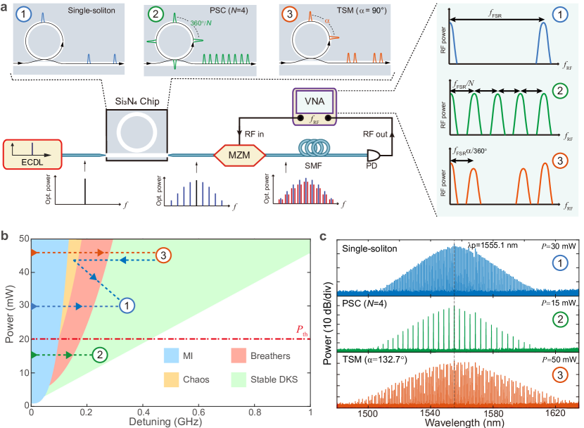
Figure 1: Schematic diagram of reconfigurable soliton based RF photonic filters and their underlying microcomb generation. a, The conceptual setup consists of four parts: microcomb generation, RF signal upconversion, dispersive propagation, and photodetection. ECDL: external cavity diode laser; MZM: Mach-Zehnder modulator; SMF: single mode fiber; PD: photodiode; VNA: vector network analyzer. Various RF filters are synthesized based on versatile soliton microcombs: (1) single-soliton based RF filter with passband centered at $f_{\mathrm{FSR}}$ (blue); (2) $N-$PSC (perfect soliton crystals of $N$ equally spaced solitons within one round-trip) based RF filters with passband centered at $f_{\mathrm{FSR}}/N$ (green, $N=4$ is shown); (3) Two-soliton microcomb (TSM) based RF filters with passband centered at $f_{\mathrm{FSR}}{\alpha}/360^{\circ}$ (orange), where $\alpha$ is the relative azimuthal angle between two solitons ($\alpha=90^{\circ}$ is shown). b, Simulated stability diagram of the Lugiato–Lefever equation (LLE) involving the experimental avoided mode crossing (AMX) condition. Four different stability regions are listed: modulation instability (MI, blue), breathers (red), spatio-temporal and transient chaos (chaos, yellow), and stable dissipative Kerr soliton (DKS, green). PSC and TSM/single-soliton spectra are obtained by distinct approaches. PSC states are accessed under the threshold power to avoid the chaos region. Single-soliton or TSM states are accessed above the threshold power, by either directly falling to the states or backward tuning from higher number of solitons. c, Examples of experimentally generated spectra at resonance of ${1555.1\leavevmode\nobreak\ {\rm nm}}$: (1) single-soliton, (2) PSC (N=4), and (3) TSM ($\alpha=132.7^{\circ}$). The corresponding pump power is also shown for each microcomb generation.

In this paper, we demonstrate for the first time, to our knowledge, soliton microcomb based RF photonic filters without any external pulse shaping. In addition, the synthesized RF filters can be all-optically reconfigured through the internal versatile soliton states. Specifically, we trigger, in a deterministic fashion, the perfect soliton crystals (PSC) to multiply the comb spacing karpov2019dynamics ; 2019arXiv191000114H , thereby dividing the RF passband frequencies. Moreover, a completely new regime of filter reconfiguration is achieved based on versatile two-soliton microcombs (TSM). The spectral interference of two solitons is functionally equivalent to an interferometric setup, shifting the filter passband frequency via modification of the angle between them. A proof-of-concept filter reconfiguration experiment is also shown using TSM based RF filters. The internal exploitation of abundant and regulated soliton formats of microresonator effectively bypasses the need of another programmable pulse shaper and interferometric setup for RF filter tuning xue2014programmable ; xu2019advanced . Thus, the proposed scheme dramatically reduces the system complexity and form factor of microcomb based RF filters, and are readily applicable to the current radar systems, 5G wireless, and satellite communications.

Figure 1a illustrates the conceptual setup for soliton microcomb based RF filters. Firstly, a telecom C-band continuous wave (CW) laser initiates microcomb generation, where each comb line serves as the RF filter tap. By modulating the RF signals from a vector network analyzer (VNA) on an electro-optic Mach-Zehnder modulator (MZM), the RF signals are broadcast to each microcomb mode. Then the upconverted signals are propagated through a spool of single mode fiber (SMF) to acquire incremental delay between filter taps. Finally, the signals are converted back to RF domain in a fast photodetector (PD). The detailed experimental setup is described in the Methods. This arrangement exactly corresponds to a TDL filter, where the power of each comb line $p_{k}$ is the tap weight, and the delay is determined by the comb spacing $f_{m}$ and the accumulated dispersion $\phi_{2}=-{\beta_{2}}L$ (the product of SMF second-order dispersion $\beta_{2}$ and fiber length $L$). When the filter tap weights take the ${\rm sech^{2}}$ envelope of a single-soliton comb (case 1), the RF filter response is given as (see Supplementary Information):

$$H({f_{\mathrm{RF}}})\sim\cos(2\pi^{2}{\phi_{2}}{f_{\mathrm{RF}}^{2}})\sum_{n=-\infty}^{\infty}G(f_{\mathrm{RF}}-n{f_{\mathrm{FSR}}})$$ (1)

where $f_{\mathrm{FSR}}$ and $G(f_{\mathrm{RF}})$ are respectively defined as $1/(2\pi{\phi_{2}}{f_{m}})$ and $2\frac{T}{T_{0}}\frac{f_{\mathrm{RF}}}{f_{\mathrm{FSR}}}{\operatorname{sinh}^{-1}(\frac{T}{T_{0}}\frac{f_{\mathrm{RF}}}{f_{\mathrm{FSR}}})}$, with $T=1/f_{m}$ the repetition period, and $T_{0}$ the soliton pulse width. $f_{\mathrm{RF}}$ denotes the RF frequency. Notice that higher order dispersion of SMF is neglected here to give a more intuitive picture. The overall RF filter response can be seen as a periodic function of lineshape $G(f_{\mathrm{RF}})$ with RF free spectral range (FSR) of $f_{\mathrm{FSR}}$, modulated by a envelope due to the double-sideband (DSB) modulation scheme being used. As the tap weights are all-positive, the passband frequencies of the RF filters are at every multiples of $f_{\mathrm{FSR}}$, including a DC response. Throughout this letter, we focus on the first passband.

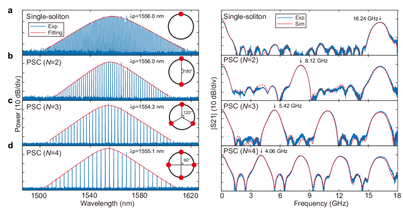
Figure 2: Single-soliton/PSC spectra and their corresponding RF photonic filters. Through deterministic accessing PSC states of different resonances, the RF filter passbands can be divided correspondingly. Left column: microcomb spectra (blue: experiment, red: ${\rm sech^{2}}$ fitting); Right column: corresponding normalized RF filter responses (blue: experiment, red: simulation). a, RF filter centered at ${16.24\leavevmode\nobreak\ {\rm GHz}}$ based on single-soliton from resonance of ${1556.0\leavevmode\nobreak\ {\rm nm}}$; b-d, RF filters centered at ${8.12\leavevmode\nobreak\ {\rm GHz}}$, ${5.42\leavevmode\nobreak\ {\rm GHz}}$, and ${4.06\leavevmode\nobreak\ {\rm GHz}}$ based on ${2-}$, ${3-}$, ${4-}$times PSC, generated at resonances of ${1556.0\leavevmode\nobreak\ {\rm nm}}$, ${1554.3\leavevmode\nobreak\ {\rm nm}}$, ${1555.1\leavevmode\nobreak\ {\rm nm}}$, respectively. The insets of left column illustrate soliton distribution inside the microresonator: a single-soliton; b-d equally spaced solitons (PSC) with adjacent angles of $180^{\circ}$, $120^{\circ}$, and $90^{\circ}$, respectively $(360^{\circ}/N,N=2,3,4)$.

Besides, by exploiting the rich soliton states of microresonator, the RF filters can be easily reconfigured at no additional cost nor complexity. Among soliton crystal structurescole2017soliton ; wang2018robust , the defect-free PSC is of particular interest, as $N(N\in N_{+}\mid N\geq 2)$ equally-spaced solitons (case 2) within one roundtrip time simply multiplies the initial comb spacing by $N$-times. This imparts $N$-times division of the filter passband frequencies, while preserving the filter bandwidth. The automatic PSC control is equivalent to the Talbot-based processer for discrete programming the RF filters in ref maram2019discretely . Less intuitively, all-optical reshaping of the RF filters can also be achieved via versatile TSM spectra (case 3). Two solitons residing in one period induce sinusoid interference on the ${\rm sech^{2}}$ spectral shape of a soliton, modulating the tap weights of the TDL filter. This rewrites the RF filter response as (see Supplementary Information):

$$H({f_{\mathrm{RF}}})\sim\cos(2\pi^{2}{\phi_{2}}{f_{\mathrm{RF}}^{2}})[\sum_{n=-\infty}^{\infty}2G(f_{\mathrm{RF}}-n{f_{\mathrm{FSR}}})$$ (2)

$$G(f_{\mathrm{RF}}-(n-\frac{{\alpha}}{2\pi})f_{\mathrm{FSR}})+G(f_{\mathrm{RF}}-(n+\frac{{\alpha}}{2\pi})f_{\mathrm{FSR}})]$$

where $\alpha$ is the relative azimuthal angle between two solitons (expressed in radian for calculation). Clearly, new RF passbands of halved amplitude appear due to two-soliton interference, which are displaced at both sides from the initial response according to the azimuthal angle between them. Thus, the RF filter passbands can slide inside $f_{\mathrm{FSR}}$ by modifying the relative soliton angles. Unlike ref xu2019advanced in which the authors artificially introduce the sinusoidal modulation via programming the spectral carving, we alleviate the need for a pulse shaper and realize sinusoidal modulation by directly generating a series of TSM spectra. This novel scheme achieves for the first time wideband reconfiguration of RF filters without either interferometric configuration or additional pulse shaping.

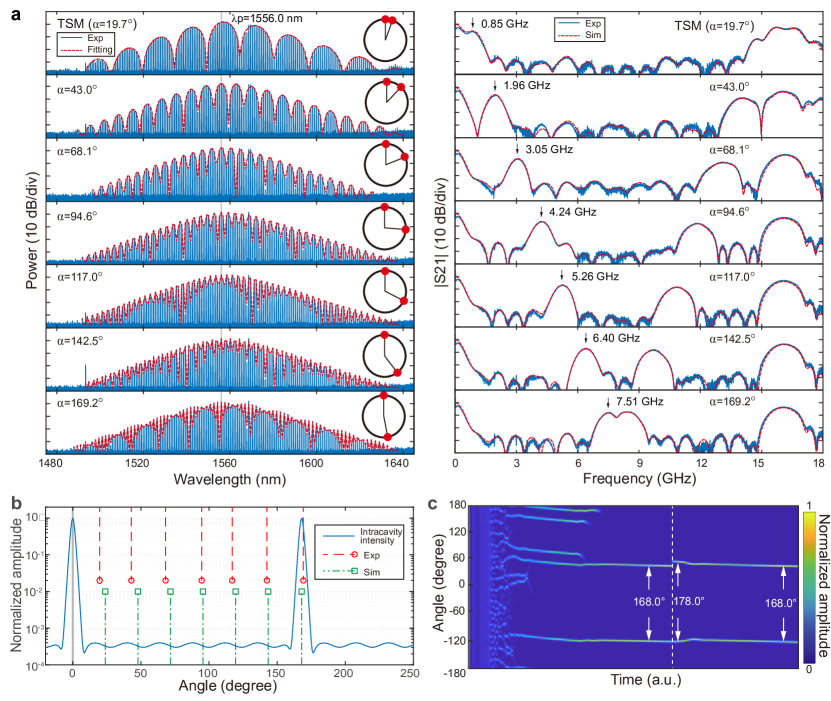
Figure 3: TSM spectra and their corresponding RF photonic filters, together with TSM simulation investigation. By accessing different two-soliton states, the RF filters can be all-optically reconfigured. a, Left column: TSM spectra at resonance of ${1555.96\leavevmode\nobreak\ {\rm nm}}$ (blue: experiment, red: envelope fitting). The insets illustrate two soliton distribution inside the microresonator: the angles between them are $19.7^{\circ}$, $43.0^{\circ}$, $68.1^{\circ}$, $94.6^{\circ}$, $117.0^{\circ}$, $142.5^{\circ}$, and $169.2^{\circ}$, respectively. Right column: corresponding normalized RF filter responses (blue: experiment, red: simulation) with passbands at ${0.85}$, ${1.96}$, ${3.05}$, ${4.24}$, ${5.26}$, ${6.40}$, and ${7.51\leavevmode\nobreak\ {\rm GHz}}$, respectively. b, Simulation of TSM relative azimuthal angles. One example of the simulated TSM intracavity intensity profile (blue), where AMX induced background modulation is observed. The red and green lines respectively indicate measured and simulated possible relative angles between two solitons. c, Simulation of the intracavity waveform evolution of TSM for robustness test. First, TSM state with relative angle of $168.0^{\circ}$ is excited by scanning the pump over the resonance. Once the TSM becomes stable, a $10.0^{\circ}$ perturbation is introduced to one of the solitons at white dashed line. The relative angle will re-stabilize to the original angle of $168.0^{\circ}$ after a period of free running.

The soliton microcombs used for RF filtering are generated from an ${104\leavevmode\nobreak\ {\rm GHz}}$ ultra-low loss integrated silicon nitride (Si₃N₄) microresonator (Q $\sim 1\times 10^{7}$), fabricated by the photonic Damascene reflow process liu2018ultralow . By employing the frequency-comb-assisted diode laser spectroscopy, the detailed properties of resonances and the integrated group velocity dispersion (GVD) of the microresonator are measured (see Supplementary Information). Strong avoided mode crossings (AMX) are observed around ${1565\leavevmode\nobreak\ {\rm nm}}$, which lead to the modulation of intracavity CW background, thereby resulting in the ordering of the DKS pulses wang2017universal and the formation of soliton crystals karpov2019dynamics ; cole2017soliton ; wang2018robust . Figure 1b shows the simulated stability diagram (see Methods), which consists of modulation instability (MI), breathers, chaos (spatio-temporal chaos and transient chaos), and stable DKS states. Additionally, it has been revealed that the pump power level is critical for whether the PSC or stochastic DKS states are formed karpov2019dynamics . In our case, the threshold pump power $P_{\mathrm{th}}$ is found to be around $20\leavevmode\nobreak\ {\rm mW}$ in the bus waveguide. When the laser scanning route is operated below threshold pump power, PSC states can be accessed without crossing the chaos region. Contrarily, DKS states with stochastic soliton number are accessed above the threshold power. Experimentally, the single soliton and TSM states are obtained by either directing falling to the states or backward tuning from the states with higher soliton number guo2017universal . Thus, through controlling the pump power and resonance frequency, various soliton microcombs (single-soliton, PSC, and TSM) can be obtained on demand to produce the desired RF filter responses. For example, Figure 1c shows three distinct optical spectra obtained from the resonance of ${1555.1\leavevmode\nobreak\ {\rm nm}}$: single soliton, PSC ($N=4$), and TSM ($\alpha=132.7^{\circ}$), respectively.

Figure 2 depicts the RF photonic filters using single soliton and various PSC microcombs. The single-soliton based RF filter (Figure 2a) is centered at ${16.24\leavevmode\nobreak\ {\rm GHz}}$, with main-to-sidelobe suppression ratio (MSMR) of ${23.2\leavevmode\nobreak\ {\rm dB}}$. Further, various PSC states are deterministically obtained at different resonances under the threshold power, thereby all-optically reconfiguring the corresponding RF filters. The comb spacing multiplication via PSC results in the division of the corresponding RF passbands. RF filters centered at ${8.12\leavevmode\nobreak\ {\rm GHz}}$, ${5.42\leavevmode\nobreak\ {\rm GHz}}$, and ${4.06\leavevmode\nobreak\ {\rm GHz}}$ (Figure 2b-d) are experimentally synthesized through $2$, $3$, and $4$ equally spaced solitons, with MSMR of ${22.6\leavevmode\nobreak\ {\rm dB}}$, ${25.6\leavevmode\nobreak\ {\rm dB}}$, and ${20.4\leavevmode\nobreak\ {\rm dB}}$, respectively. All these RF filters achieve MSMR over ${20\leavevmode\nobreak\ {\rm dB}}$ without additional programmable spectral shaping. The MSMR here are limited by the smoothness of the optical spectra supradeepa2012comb , as several AMX can be seen in the microcombs. Nevertheless, all these microcombs preserve well the $sech^{2}$ envelope, and remained smooth after amplification. In addition, the measured RF filter responses are in excellent agreement with simulations, by taking into account of third-order dispersion ($\beta_{3}$) of SMF (see Methods). The bandwidth of the RF filters are respectively ${1060\leavevmode\nobreak\ {\rm MHz}}$, ${755\leavevmode\nobreak\ {\rm MHz}}$, ${690\leavevmode\nobreak\ {\rm MHz}}$, and ${645\leavevmode\nobreak\ {\rm MHz}}$, which scale inversely with their center frequencies, also due to the third-order dispersion of SMF xue2014programmable .

Figure 3a shows the TSM spectra and their corresponding RF filter responses, pumped at resonance of ${1556.0\leavevmode\nobreak\ {\rm nm}}$. According to Eq. (2), the first passband frequencies of RF filters scale linearly with the relative angles between two solitons, so that the filter reconfiguration is achieved. In the experiment, TSM spectra with relative angles of $19.7^{\circ}$, $43.0^{\circ}$, $68.1^{\circ}$, $94.6^{\circ}$, $117.0^{\circ}$, $142.5^{\circ}$, and $169.2^{\circ}$ are obtained, where the angles are extracted from the fitting of the microcomb spectral envelope (see Methods). The measured RF filters are correspondingly centered at ${0.85\leavevmode\nobreak\ {\rm GHz}}$, ${1.96\leavevmode\nobreak\ {\rm GHz}}$, ${3.05\leavevmode\nobreak\ {\rm GHz}}$, ${4.24\leavevmode\nobreak\ {\rm GHz}}$, ${5.26\leavevmode\nobreak\ {\rm GHz}}$, ${6.40\leavevmode\nobreak\ {\rm GHz}}$, and ${7.51\leavevmode\nobreak\ {\rm GHz}}$, confirming the linear relation with the soliton angle. As in the case of PSC, a slight broadening of the filter passband width from ${490\leavevmode\nobreak\ {\rm MHz}}$ to ${620\leavevmode\nobreak\ {\rm MHz}}$ is attributed to the third-order dispersion of SMF. Overall, the RF filters obtained at resonance ${1555.96\leavevmode\nobreak\ {\rm nm}}$ could vary from DC to ${8.1\leavevmode\nobreak\ {\rm GHz}}$ ($f_{\mathrm{FSR}}/2$) with maximum grid of ${1.2\leavevmode\nobreak\ {\rm GHz}}$, while roughly preserving the filter bandwidth in the meantime. The granularity of TSM based RF filters can be further reduced to less than ${1\leavevmode\nobreak\ {\rm GHz}}$ by exploiting adjacent resonances of ${1556.0\leavevmode\nobreak\ {\rm nm}}$ (see Supplementary Information).

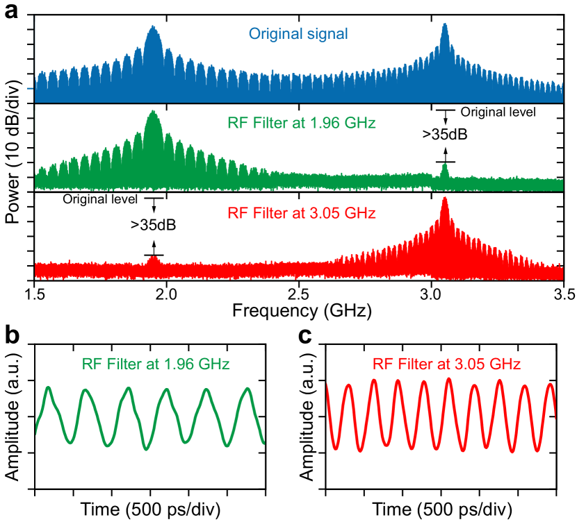
Figure 4: Proof-of-concept experiment using TSM based RF filters. Two PSK signals with ${40\leavevmode\nobreak\ {\rm Mb/s}}$ modulation at ${1.96\leavevmode\nobreak\ {\rm GHz}}$ and ${20\leavevmode\nobreak\ {\rm Mb/s}}$ modulation at ${3.05\leavevmode\nobreak\ {\rm GHz}}$, are filtered by the TSM based RF filters centered at ${1.96\leavevmode\nobreak\ {\rm GHz}}$ and ${3.05\leavevmode\nobreak\ {\rm GHz}}$, respectively. a Electrical spectra (from top to bottom) of original signal, signal after ${1.96\leavevmode\nobreak\ {\rm GHz}}$ filter, and signal after ${3.05\leavevmode\nobreak\ {\rm GHz}}$ filter. b Waveform after ${1.96\leavevmode\nobreak\ {\rm GHz}}$ filter. c Waveform after ${3.05\leavevmode\nobreak\ {\rm GHz}}$ filter.

Importantly, the possible angles between two solitons are determined by the overall AMX profile, and are rather robust to both laser power and frequency detuning, thereby deterministically dictating the filter passband frequencies to be either one of those shown in Figure 3a. To gain insights of the relative angles between two solitons, we also perform perturbed Lugiato–Lefever equation (LLE) simulation to investigate the TSM formations (see Methods). The blue curve in Figure 3b shows one example of the steady state two-soliton temporal intracavity profile. Due to the AMX effect, periodic intensity modulation is observed upon the CW background. It is clearly seen that the soliton can only be excited at specific parameter gradients wang2017universal , as manifested by the green dashed lines which correspond to the stationary solutions obtained in simulation. These possible soliton angles are in good agreement with experimental results, indicated as red dashed lines. To further test the robustness of the angle between two solitons, an external perturbation is deliberately introduced on their relative angle. Figure 3c illustrates the dynamical evolution of the two-soliton formation. The simulation is initiated as a standard laser scanning scheme to kick out two solitons. Once the simulation reaches stable two-soliton solution (relative angle of $168.0^{\circ}$), one of the solitons is dragged from its original position by a $10.0^{\circ}$ on purpose. After a period of free running, the two solitons converge back to their original relative positions, again at $168.0^{\circ}$ apart. This confirms the regulation of two solitons under AMX background modulation.

A proof-of-concept RF filter reconfiguration experiment is also illustrated in Figure 4 using TSM based RF filters (see Methods). Two superimposed phase-shift keying (PSK) signals in which a ${40\leavevmode\nobreak\ {\rm Mb/s}}$ modulation at ${1.96\leavevmode\nobreak\ {\rm GHz}}$ tone and a ${20\leavevmode\nobreak\ {\rm Mb/s}}$ modulation at ${3.05\leavevmode\nobreak\ {\rm GHz}}$ tone, are prepared as input test signals. The RF filters are then respectively reconfigured at ${1.96\leavevmode\nobreak\ {\rm GHz}}$ and ${3.05\leavevmode\nobreak\ {\rm GHz}}$ to filter the input signals, by triggering the TSM spectra of corresponding soliton angles. At the output of the RF filters, nearly complete rejection of either one of the PSK signals is observed on the electrical spectra (Figure 4a), where the extinction ratio exceeds ${35\leavevmode\nobreak\ {\rm dB}}$ for both cases. Figure 4b-c show the filtered output RF waveforms. The periodicity of the output temporal traces corroborate the filtering of the original RF signals.

In conclusion, we demonstrate reconfigurable soliton based RF photonic filters using simple approaches. Contrary to previous demonstrations where pulse shapers are necessitate to obtain descent passband responses xue2014programmable ; xu2019advanced ; xu2019high , the proposed schemes are intrinsically well-shaped with the smooth spectral envelope of solitons. More importantly, we harness various intrinsic DKS states of microresonator, like PSC and TSM, for RF filter reconfiguration at no additional cost. The diversity and regularization of soliton formats in microresonator are investigated in the favor of RF photonic filters. To certain extent, these inherent soliton states could be in place of substantial efforts made in the past for reconfiguring the comb based RF filters, such as using interferometric architecture supradeepa2012comb ; xue2014programmable , programmable pulse shaping zhu2017novel ; xu2019advanced , or Talbot-based signal processor maram2019discretely . Nevertheless, subjected to the same challenges of any other comb based RF filters, our current filters are not yet optimized in terms of the link performance. While the noise reduction and gain enhancement could be achieved using high power-handling balanced detectors kim2014comb . Besides, the recent advancement on the integration between laser chip and microresonator stern2018battery ; raja2019electrically , as well as replacing the SMF with a highly dispersive integrated waveguide sancho2012integrable , can be further connected to the current work for miniaturization. To conclude, our work significantly reduces the system complexity, size, and cost of the microcomb based RF filters, while preserving their wide reconfigurability. The proposed schemes set as a stepping stone for chipscale, cost-effective, and widely reconfigurable microcomb based RF filters.

Methods

Experimental setup: A C-band tunable CW laser is amplified by an Erbium-doped fiber amplifier (EDFA) with amplified spontaneous emission (ASE) filtered, polarization aligned at the TE mode, and then coupled to the ${\rm Si_{3}N_{4}}$ microresonator for soliton microcomb generation. The input and output coupling of the chip is achieved via lensed fibers of around ${30\%}$ fiber-chip-fiber coupling efficiency. The soliton microcombs are initiated by scanning the pump over the resonances, with the assistance of an arbitrary function generator (AFG) herr2014temporal . The residual pump of generated microcombs are then filtered by a tunable fiber Bragg grating (FBG), while a circulator is inserted in between to avoid back-reflection. ${10\%}$ of light is tapped to an optical spectrum analyzer (OSA) to record the microcomb spectra. The other ${90\%}$ of the light is amplified, and polarization managed, before sending to a ${30\leavevmode\nobreak\ {\rm GHz}}$ bandiwdth MZM. RF signals from the VNA are applied to the MZM in DSB modulation format. The modulated spectra are then propagated through a spool of ${4583.8\leavevmode\nobreak\ {\rm m}}$ SMF to acquire dispersive delays, and finally beats at a ${18\leavevmode\nobreak\ {\rm GHz}}$ PD to convert the signals back to the RF domain. The length of SMF is measured by a commercial optical time-domain reflectometer (OTDR).

For the system demonstration, a ${12\leavevmode\nobreak\ {\rm GSa/s}}$ arbitrary waveform generator (AWG) is used to prepare the input RF signals. ${40\leavevmode\nobreak\ {\rm Mb/s}}$ PSK signal modulated at ${1.96\leavevmode\nobreak\ {\rm GHz}}$ tone and ${20\leavevmode\nobreak\ {\rm Mb/s}}$ PSK signal modulated at ${3.05\leavevmode\nobreak\ {\rm GHz}}$ tone, are generated separately from the two channels of the AWG. After adding the two streams of signals in a combiner, the composite signal is then sent through the TSM based RF filters, tuned at ${1.96\leavevmode\nobreak\ {\rm GHz}}$ and ${3.05\leavevmode\nobreak\ {\rm GHz}}$, respectively. The output spectra are measured by a electrical spectrum analyzer (ESA), while the waveforms are measured using a high-speed real-time oscilloscope.

Si₃N₄ microresonator: The Si₃N₄ microresonator used in the experiment is a ring structure with radius of $217\leavevmode\nobreak\ {\rm\mu m}$. Its waveguide cross section (width $\times$ height), is made to be $1500\leavevmode\nobreak\ {\rm nm}\times 750\leavevmode\nobreak\ {\rm nm}$. The microresonator is coupled with a bus waveguide, which possesses the same cross section as the ring to realize high coupling idealityliu2018ultralow . To achieve critical coupling for the resonances, the gap distance between the ring and bus waveguide is designed to be $690\leavevmode\nobreak\ {\rm nm}$. In our experiment, the pumped resonances are around $1556\leavevmode\nobreak\ {\rm nm}$, where both the intrinsic linewidths and coupling strengths are approximately $20\leavevmode\nobreak\ {\rm MHz}$ (see Supplementary Information). With respect to the reference resonance of $\omega_{0}/2\pi=192.8\leavevmode\nobreak\ {\rm THz}$, the dispersion parameters of microresonator are measured: FSR of microresonator $D_{1}/2\pi\approx 103.9\leavevmode\nobreak\ {\rm GHz}$, second-order dispersion term $D_{2}/2\pi\approx 1.28\leavevmode\nobreak\ {\rm MHz}$, and negligible third-order dispersion term $D_{3}/2\pi\sim\mathcal{O}(1)\leavevmode\nobreak\ {\rm kHz}$ (see Supplementary Information).

LLE Simulation: The simulation performed in this work is based on the perturbed LLE model:

$$\frac{\partial A(\phi,t)}{\partial t}= -(\frac{\kappa}{2}+j(\omega_{0}-\omega_{p}))A(\phi,t)+j\frac{D_{2}}{2}\frac{\partial^{2}A(\phi,t)}{\partial\phi^{2}}$$ (3)

$$+jg|A(\phi,t)|^{2}A(\phi,t)+\sqrt{\kappa_{\mathrm{ex}}}s_{\mathrm{in}}$$

where $A(\phi,t)$ is the temporal envelope of the intracavity field. $\kappa=\kappa_{\mathrm{ex}}+\kappa_{0}$ is the total cavity loss rate, where $\kappa_{\mathrm{ex}}$ is the coupling rate, and $\kappa_{0}$ is the internal loss rate. $\omega_{0}$ and $\omega_{p}$ denote the angular frequencies of the pumped resonance and the CW pump laser, respectively. $g$ is the Kerr frequency shift per photon, defined as $g=\hbar\omega_{0}^{2}cn_{2}/n_{0}^{2}V_{\mathrm{eff}}$, where $n_{0}$ is the effective group refractive index, $n_{2}$ is the nonlinear optical index, and $V_{\mathrm{eff}}$ is the effective mode volume. $D_{2}$ corresponds to the second-order dispersion term, and $|s_{\mathrm{in}}|^{2}$ is the pump power. To involve the AMX effect, an additional frequency detuning $\Delta_{k}$ is introduced at the $k$-th mode, so that the frequency of the $k$-th mode becomes $\omega_{k}=\omega_{0}+D_{1}k+D_{2}k^{2}/2+\Delta_{k}$ (see Supplementary Information). Here in simulation, the dispersion is limited to $D_{2}$, and the Raman and thermal effects are not taken into account. According to the dispersion measurement and the generated microcomb spectra, the parameters for the AMX in the simulation are set as $k=15$ and $\Delta_{k}/2\pi=100\leavevmode\nobreak\ \mathrm{MHz}$, enabling the modulation of the CW intracavity background for the trapping of soliton temporal positions. Note that the strength of the AMX here is estimated to introduce the regularizability of solitons, but without disturbing their formationskarpov2019dynamics . Other parameters used in the simulation are retrieved from the characterization, that is, $D_{1}/2\pi=103.9\leavevmode\nobreak\ \mathrm{GHz}$, $D_{2}/2\pi=1.28\leavevmode\nobreak\ \mathrm{MHz}$, $\kappa_{\mathrm{ex}}/{2\pi}=\kappa_{0}/{2\pi}=\kappa/{4\pi}=20\leavevmode\nobreak\ \mathrm{MHz}$.

The simulation of stability chart is obtained by initializing the numerical model with single-soliton solution at various pump power and detuning conditions karpov2019dynamics . Four different states are found: MI, breathers, spatiotemporal and transient chaos, and stable DKS states. The threshold pump power, separating the PSC and stochastic DKS formations, is estimated from both the simulation and experimental results. For the TSM simulation, the numerical model is operated under standard CW laser pump scanning from blue-detuned to red-detuned side, until it reaches the stable TSM states. All the possible angles of TSM are recorded. To test the robustness of the TSM azimuthal angle, the model is initialized with one of the exact two-soliton solution but deliberately perturbed by $10^{\circ}$ angle deviation. Two solitons are gradually re-stabilized at its original azimuthal angle after a period of free runing.

RF filter response fitting: As the generated microcomb spectra are broader than the amplifying bandwidth of EDFA, we also measured the optical spectra after the EDFA, in order to extract the TDL filter tap weights. The third-order dispersion $\beta_{3}$ of SMF is taken into account for the fitting of RF responses, which can be formulated as zhu2017novel :

$$H({f_{\mathrm{RF}}})\sim\sum_{k}{p_{k}}\cos(2\pi^{2}{\phi_{2}}{f_{\mathrm{RF}}^{2}}+4\pi^{3}{\phi_{3}}k{f_{m}^{2}}{f_{\mathrm{RF}}})\times$$ (4)

$$\exp(j{4\pi^{2}}{\phi_{2}}k{f_{m}}{f_{\mathrm{RF}}}+j{4\pi^{3}}{\phi_{3}}{k^{2}}{f_{m}^{2}}{f_{\mathrm{RF}}}+j\frac{4}{3}{\pi^{3}}{\phi_{3}}{f_{m}^{3}})$$

where $\phi_{3}=-{\beta_{3}}L$. In accordance with typical values of SMF dispersion, ${\beta_{2}}=-20.2\leavevmode\nobreak\ {\rm ps^{2}/km}$ and ${\beta_{3}}=0.117\leavevmode\nobreak\ {\rm ps^{3}/km}$ at $1550\leavevmode\nobreak\ {\rm nm}$ are estimated for all the above fittings of RF filters. The simulation results are in excellent agreement with experimental RF filter responses.

TSM spectral fitting: First, we extract the power of each comb mode of experimental TSM spectra, and indexed them with respect to the pump mode. Pump mode is rejected and amplitude rescaling is considered as a fitting parameter. Note that the amount of spectral red-shift due to Raman effect is also estimated in fitting, by displacing the center of ${\rm sech^{2}}$ soliton spectra from the pump comb mode. Then, the rescaling parameter and red-shift are estimated to best fit the experimental data with the TSM spectral power equation (see Supplementary Information), thereby retrieving the azimthual angle $\alpha$ between two solitons. Excellent match between simulations and experimental spectra are obtained.

Funding Information: This work was supported by Contract HR0011-15-C-0055 (DODOS) from the Defense Advanced Research Projects Agency (DARPA), Microsystems Technology Office (MTO), and by the Air Force Office of Scientific Research, Air Force Material Command, USAF under Award No. FA9550-19-1-0250, and by Swiss National Science Foundation under grant agreement No. 176563 (BRIDGE), No.165933 and No. 159897.

Acknowledgments: The Si₃N₄ microresonator samples were fabricated in the EPFL center of MicroNanoTechnology (CMi).

Data Availability Statement: The code and data used to produce the plots within this work will be released on the repository Zenodo upon publication of this preprint.

References

- (1) Xue, X. et al. Programmable single-bandpass photonic rf filter based on kerr comb from a microring. Journal of Lightwave Technology 32, 3557–3565 (2014). URL https://doi.org/10.1109/jlt.2014.2312359.
- (2) Xu, X. et al. Advanced adaptive photonic rf filters with 80 taps based on an integrated optical micro-comb source. Journal of Lightwave Technology 37, 1288–1295 (2019). URL https://doi.org/10.1109/jlt.2019.2892158.
- (3) Xu, X. et al. High performance rf filters via bandwidth scaling with kerr micro-combs. APL Photonics 4, 026102 (2019). URL https://doi.org/10.1063/1.5080246.
- (4) Karpov, M. et al. Dynamics of soliton crystals in optical microresonators. Nature Physics 1–7 (2019). URL https://doi.org/10.1038/s41567-019-0635-0.
- (5) Wang, Y. et al. Universal mechanism for the binding of temporal cavity solitons. Optica 4, 855–863 (2017). URL https://doi.org/10.1364/optica.4.000855.
- (6) Capmany, J. & Novak, D. Microwave photonics combines two worlds. Nature photonics 1, 319 (2007). URL https://doi.org/10.1038/nphoton.2007.89.
- (7) Marpaung, D., Yao, J. & Capmany, J. Integrated microwave photonics. Nature photonics 13, 80 (2019). URL https://doi.org/10.1038/s41566-018-0310-5.
- (8) Sancho, J. et al. Integrable microwave filter based on a photonic crystal delay line. Nature communications 3, 1075 (2012). URL https://doi.org/10.1038/ncomms2092.
- (9) Metcalf, A. J. et al. Integrated line-by-line optical pulse shaper for high-fidelity and rapidly reconfigurable rf-filtering. Optics express 24, 23925–23940 (2016). URL https://doi.org/10.1364/oe.24.023925.
- (10) Zhuang, L., Roeloffzen, C. G., Hoekman, M., Boller, K.-J. & Lowery, A. J. Programmable photonic signal processor chip for radiofrequency applications. Optica 2, 854–859 (2015). URL https://doi.org/10.1364/optica.2.000854.
- (11) Marpaung, D. et al. Si 3 n 4 ring resonator-based microwave photonic notch filter with an ultrahigh peak rejection. Optics express 21, 23286–23294 (2013). URL https://doi.org/10.1364/oe.21.023286.
- (12) Eggleton, B. J., Poulton, C. G., Rakich, P. T., Steel, M. J. & Bahl, G. Brillouin integrated photonics. Nature Photonics 1–14 (2019). URL https://doi.org/10.1038/s41566-019-0498-z.
- (13) Fandiño, J. S., Muñoz, P., Doménech, D. & Capmany, J. A monolithic integrated photonic microwave filter. Nature Photonics 11, 124 (2017). URL https://doi.org/10.1038/nphoton.2016.233.
- (14) Capmany, J., Ortega, B. & Pastor, D. A tutorial on microwave photonic filters. Journal of Lightwave Technology 24, 201–229 (2006). URL https://doi.org/10.1109/jlt.2005.860478.
- (15) Supradeepa, V. et al. Comb-based radiofrequency photonic filters with rapid tunability and high selectivity. Nature Photonics 6, 186 (2012). URL https://doi.org/10.1038/nphoton.2011.350.
- (16) Maram, R., Onori, D., Azaña, J. & Chen, L. R. Discretely programmable microwave photonic filter based on temporal talbot effects. Optics express 27, 14381–14391 (2019). URL https://doi.org/10.1364/oe.27.014381.
- (17) Zhu, X., Chen, F., Peng, H. & Chen, Z. Novel programmable microwave photonic filter with arbitrary filtering shape and linear phase. Optics express 25, 9232–9243 (2017). URL https://doi.org/10.1364/oe.25.009232.
- (18) Xue, X. et al. Microcomb-based true-time-delay network for microwave beamforming with arbitrary beam pattern control. Journal of Lightwave Technology 36, 2312–2321 (2018). URL https://doi.org/10.1109/jlt.2018.2803743.
- (19) Xu, X. et al. Broadband rf channelizer based on an integrated optical frequency kerr comb source. Journal of Lightwave Technology 36, 4519–4526 (2018). URL https://doi.org/10.1109/jlt.2018.2819172.
- (20) Tan, M. et al. Microwave and rf photonic fractional hilbert transformer based on a 50ghz kerr micro-comb. Journal of Lightwave Technology (2019). URL https://doi.org/10.1109/jlt.2019.2946606.
- (21) Xue, X. et al. Mode-locked dark pulse kerr combs in normal-dispersion microresonators. Nature Photonics 9, 594 (2015). URL https://doi.org/10.1038/nphoton.2015.137.
- (22) Herr, T. et al. Temporal solitons in optical microresonators. Nature Photonics 8, 145 (2014). URL https://doi.org/10.1038/nphoton.2013.343.
- (23) Stern, B., Ji, X., Okawachi, Y., Gaeta, A. L. & Lipson, M. Battery-operated integrated frequency comb generator. Nature 562, 401 (2018). URL https://doi.org/10.1038/s41586-018-0598-9.
- (24) Raja, A. S. et al. Electrically pumped photonic integrated soliton microcomb. Nature communications 10, 680 (2019). URL https://doi.org/10.1038/s41467-019-08498-2.
- (25) Marin-Palomo, P. et al. Microresonator-based solitons for massively parallel coherent optical communications. Nature 546, 274 (2017). URL https://doi.org/10.1038/nature22387.
- (26) Suh, M.-G. & Vahala, K. J. Soliton microcomb range measurement. Science 359, 884–887 (2018). URL https://doi.org/10.1126/science.aao1968.
- (27) Suh, M.-G., Yang, Q.-F., Yang, K. Y., Yi, X. & Vahala, K. J. Microresonator soliton dual-comb spectroscopy. Science 354, 600–603 (2016). URL https://doi.org/10.1126/science.aah6516.
- (28) Obrzud, E. et al. A microphotonic astrocomb. Nature Photonics 13, 31 (2019). URL https://doi.org/10.1038/s41566-018-0309-y.
- (29) Liu, J. et al. Nanophotonic soliton-based microwave synthesizers. arXiv e-prints arXiv:1901.10372 (2019). URL https://arxiv.org/abs/1901.10372.
- (30) He, Y., Ling, J., Li, M. & Lin, Q. Perfect soliton crystals on demand. arXiv e-prints arXiv:1910.00114 (2019). URL https://arxiv.org/abs/1910.00114.
- (31) Cole, D. C., Lamb, E. S., Del’Haye, P., Diddams, S. A. & Papp, S. B. Soliton crystals in kerr resonators. Nature Photonics 11, 671 (2017). URL https://doi.org/10.1038/s41566-017-0009-z.
- (32) Wang, W. et al. Robust soliton crystals in a thermally controlled microresonator. Optics letters 43, 2002–2005 (2018). URL https://doi.org/10.1364/ol.43.002002.
- (33) Liu, J. et al. Ultralow-power chip-based soliton microcombs for photonic integration. Optica 5, 1347–1353 (2018). URL https://doi.org/10.1364/optica.5.001347.
- (34) Guo, H. et al. Universal dynamics and deterministic switching of dissipative kerr solitons in optical microresonators. Nature Physics 13, 94 (2017). URL https://doi.org/10.1038/nphys3893.
- (35) Kim, H.-J., Leaird, D. E., Metcalf, A. J. & Weiner, A. M. Comb-based rf photonic filters based on interferometric configuration and balanced detection. Journal of Lightwave Technology 32, 3478–3488 (2014). URL https://doi.org/10.1109/jlt.2014.2326410.