Layered Superconductor in a Magnetic Field: Breakdown of the Effective Masses Model

Abstract

We theoretically study the upper critical magnetic fields at zero temperature in a quasi-two-dimensional (Q2D) superconductor in the parallel and perpendicular fields, $H_{c2}^{\parallel}(0)$ and $H_{c2}^{\perp}$(0), respectively. We find that $H_{c2}^{\parallel}(0)\approx 0.75\ |dH_{c2}^{\parallel}/dT|_{T_{c}}T_{c}$ and that $H_{c2}^{\perp}(0)\approx 0.59\ |dH_{c2}^{\perp}/dT|_{T_{c}}T_{c}$, where $|dH_{c2}^{\parallel}/dT|_{T_{c}}$ and $|dH_{c2}^{\perp}/dT|_{T_{c}}$ are the corresponding Ginzburg-Landau slopes of the upper critical magnetic fields. Our results demonstrate the breakdown of the so-called effective mass model in Q2D case and may be partially responsible for the experimentally observed deviations from the effective mass model in a number of layered superconductors, including $MgB_{2}$.

The upper critical magnetic field, $H_{c2}(T)$, is known to be one of the most important properties of the type-II superconductors. It destroys superconductivity due to the orbital Meissner currents in case, where we can disregard the Pauli spin-splitting paramagnetic effects. The Ginzburg-Landau (GL) theory gave tools to calculate a slope of the $H_{c2}(T)$ [1] in the vicinity of superconducting transition temperature, $(T_{c}-T)/T_{c}\ll 1$. On the other hand, at zero temperature, the upper critical magnetic field was calculated for an isotropic $3D$ superconductor in Ref.[2]. Temperature dependence of $H_{c2}(T)$ in a whole temperature region in an isotropic $3D$ superconductor was calculated later in Ref.[3]. Important generalization of the GL theory to the case of anisotropic superconductors was obtained in Ref.[4], where the so-called effective mass model was implicitly introduced. The effective mass model, partially based on the results obtained in Ref. [4] in the GL region, states more: ratios of the upper critical magnetic fields measured along fixed different directions do not much depend on temperature. Recently observed experimental temperature dependencies of anisotropy of the upper critical fields in layered compound MB₂ [5] and other materials are prescribed exclusively to many-band effects (see introductory part of review [6]).

The goal of our Letter is to consider the orbital effect in a parallel magnetic field in a Q2D conductor at zero temperature, where we explicitly take into account a Q2D anisotropy of the electron spectrum. In contrast to Refs.[1-4,6], we demonstrate that, in a Q2D case in a parallel magnetic field, the solution of the so-called gap equation can not be expresses as some exponential function. Moreover, we show that the above mentioned solution even changes a sign with changing space coordinate. This leads to unusual value of the corresponding coefficient, $0.75$, in the equation,

$$H_{c2}^{\parallel}(0)\approx 0.75\ |dH_{c2}^{\parallel}/dT|_{T_{c}}T_{c}\ ,$$ (1)

for a parallel magnetic field. We recall that, for a perpendicular magnetic field the corresponding solution is exponential one and gives much smaller coefficient - $0.59$ [7]:

$$H_{c2}^{\perp}(0)\approx 0.59\ |dH_{c2}^{\perp}/dT|_{T_{c}}T_{c}\ .$$ (2)

Note that Eqs.(1) and (2) directly break the effective mass model, since the corresponding coefficients, $0.75$ and $0.59$ are not close to each other. We also stress that, while deriving Eqs.(1) and (2), we do not take into account quantum effects of electron motion in a magnetic field [8-10].

In the Letter, we consider a layered superconductor with the following realistic Q2D electron spectrum:

$$\epsilon({\bf p})=\frac{1}{2m}(p^{2}_{x}+p^{2}_{y})-2t_{\perp}\cos(p_{z}c^{*})\ ,$$

$$t_{\perp}\ll\epsilon_{F}\ ,\ \ \ \ \epsilon_{F}=\frac{p^{2}_{F}}{2m}=\frac{mv^{2}_{F}}{2}\ ,$$ (3)

where $m$ - the electron in-plane mass, $t_{\perp}$ - the integral of overlapping of electron wave functions in a perpendicular to the conducting planes direction; $\epsilon_{F},\ p_{F}$, and $v_{F}$ are the Fermi energy, Fermi momentum, and Fermi velocity, correspondingly; $\hbar\equiv 1$. In a parallel to the conducting planes magnetic field,

$${\bf H}=(0,H,0)\ ,\ \ \ \ {\bf A}=(0,0,-Hx)\ ,$$ (4)

we make use of the so-called Peierls substitution method:

$$p_{x}\rightarrow-i\biggl{(}\frac{\partial}{\partial x}\biggl{)},\ \ p_{y}\rightarrow-i\biggl{(}\frac{\partial}{\partial y}\biggl{)},$$

$$c^{*}p_{z}\rightarrow-ic^{*}\biggl{(}\frac{\partial}{\partial z}\biggl{)}-\biggl{(}\frac{\omega_{c}}{v_{F}}\biggl{)}x,\ \ \omega_{c}(H)=\frac{ev_{F}c^{*}H}{c}.$$ (5)

Under such conditions the electron orbital Hamiltonian in a magnetic field can be written in the following way:

$$\hat{H}=-\frac{1}{2m}\biggl{(}\frac{\partial^{2}}{\partial x^{2}}+\frac{\partial^{2}}{\partial y^{2}}\biggl{)}-2t_{\perp}\cos\biggl{(}-ic^{*}\frac{\partial}{\partial z}-\frac{\omega_{c}}{v_{F}}x\biggl{)}.$$ (6)

As directly follows from Eq.(6), electron wave functions can be represented as

$$\Psi^{\pm}_{\epsilon}(x,y,z)=\exp[\pm ip^{0}_{x}(p_{y})x]\ \exp(ip_{y}y)\ \exp(ip_{z}z)$$

$$\times\Phi_{\epsilon}^{\pm}(x,p_{y},p_{z}),\ \ p^{0}_{x}(p_{y})=\sqrt{p_{F}^{2}-p^{2}_{y}},$$ (7)

where for main part of the Fermi surface of the Q2D electrons (3)

$$p^{0}_{x}(p_{y})\sim p_{F}.$$ (8)

Eq.(8) allows us to use quasi-classical approximation for the electron Hamiltonian (6) and electron wave function (7):

$$\frac{1}{2m}\biggl{[}\frac{p^{2}_{F}-p^{2}_{y}}{2m}\pm 2ip^{0}_{x}(p_{y})\frac{d}{dx}+\frac{p^{2}_{y}}{2m}-2t_{\perp}\cos\biggl{(}p_{z}c^{*}$$

$$-\frac{\omega_{c}}{v_{F}}x\biggl{)}\biggl{]}\ \Phi_{\epsilon}^{\pm}(x,p_{y},p_{z})=(\epsilon+\epsilon_{F})\ \Phi_{\epsilon}^{\pm}(x,p_{y},p_{z}),$$ (9)

where energy $\epsilon$ is counted from the Fermi level. It is easy to rewrite Eq.(9) in more convenient way:

$$\biggl{[}\pm iv^{0}_{x}(p_{y})\frac{d}{dx}-2t_{\perp}\cos\biggl{(}p_{z}c^{*}-\frac{\omega_{c}}{v_{F}}x\biggl{)}\biggl{]}\Phi_{\epsilon}^{\pm}(x,p_{y},p_{z})$$

$$=\epsilon\ \Phi_{\epsilon}^{\pm}(x,p_{y},p_{z}),\ \ \ v^{0}_{x}(p_{y})=p^{0}_{x}(p_{y})/m.$$ (10)

As discussed above, we consider the case of relatively small magnetic fields and high enough temperatures, where quantum effects of electron motion between the conducting planes in a magnetic field [8-10] are negligible. In this case, we can consider in Eq.(10) only the first order terms with respect to the magnetic field. As a result of this procedure, we obtain,

$$-2t_{\perp}\cos\biggl{(}p_{z}c^{*}-\frac{\omega_{c}}{v_{F}}x\biggl{)}\approx-2t_{\perp}\cos(p_{z}c^{*})$$

$$-\biggl{(}\frac{2t_{\perp}\omega_{c}x}{v_{F}}\biggl{)}\sin(p_{z}c^{*}),$$ (11)

and, therefore, Eq.(10) can be represented as

$$\biggl{[}\pm iv^{0}_{x}(p_{y})\frac{d}{dx}-2t_{\perp}\cos(p_{z}c^{*})-\biggl{(}\frac{2t_{\perp}\omega_{c}x}{v_{F}}\biggl{)}\sin(p_{z}c^{*})$$

$$-\mu_{B}\sigma H\biggl{]}\ \Phi_{\epsilon}^{\pm}(x,p_{y},p_{z};\sigma)=\epsilon\ \Phi_{\epsilon}^{\pm}(x,p_{y},p_{z};\sigma),$$ (12)

where we take into account also the Pauli spin-splitting effects in the field for spin up ($\sigma=+1$) and spin down ($\sigma=-1$), $\mu_{B}$ is the Bohr magneton. Eq.(12) can be exactly solved:

$$\Phi_{\epsilon}^{\pm}(x,p_{y},p_{z};\sigma)=\exp\biggl{(}\mp i\frac{\epsilon x}{v^{0}_{x}}\bigg{)}\exp\biggl{[}\mp i\frac{2t_{\perp}\cos(p_{z}c^{*})x}{v^{0}_{x}}\biggl{]}$$

$$\times\exp\biggl{(}\mp\frac{\mu_{B}\sigma x}{v^{0}_{x}}\biggl{)}\exp\biggl{[}\mp i\frac{t_{\perp}\omega_{c}x^{2}}{v^{0}_{x}v_{F}}\sin(p_{z}c^{*})\biggl{]}\ .$$ (13)

For Hamiltonian (12), we have the following differential equations to determine the electron Green’s functions in the mixed $(x,p_{y},p_{z})$ representation [11,12]:

$$\biggl{[}i\omega_{n}\mp iv^{0}_{x}(p_{y})\frac{d}{dx}+2t_{\perp}\cos(p_{z}c^{*})+\biggl{(}\frac{2t_{\perp}\omega_{c}x}{v_{F}}\biggl{)}\sin(p_{z}c^{*})$$

$$+\mu_{B}\sigma H\biggl{]}g_{i\omega_{n}}^{\pm}(x,p_{y},p_{z},\sigma)=\delta(x-x_{1})\ .$$ (14)

In Eq.(14), $\omega_{n}$ is the so-called Matsubara frequency [12]. Let us solve Eq.(14) analytically. As a result, for the Green’s functions we obtain:

$$g^{\pm}_{i\omega_{n}}(x,x_{1};p_{y},p_{z};\sigma)=-i\frac{sgn(\omega_{n})}{v_{x}(p_{y})}\exp\biggl{[}\mp\frac{\omega_{n}(x-x_{1})}{v_{x}(p_{y})}\biggl{]}$$

$$\times\exp\biggl{[}\pm i\frac{2t_{\perp}\cos(p_{z}c^{*})(x-x_{1})}{v^{0}_{x}}\biggl{]}\exp\biggl{[}\frac{\mp i\mu_{B}\sigma H(x-x_{1})}{v_{x}(p_{y})}\biggl{]}$$

$$\times\exp\biggl{[}\pm i\frac{t_{\perp}\omega_{c}(x^{2}-x^{2}_{1})}{v^{0}_{x}v_{F}}\sin(p_{z}c^{*})\biggl{]}.$$ (15)

Let us derive the so-called linearized Gor’kov’s equation [12] for non-uniform superconductivity to determine superconducting transition temperature as a function of a magnetic field, $T_{c}(H)$. As a result, we obtain

$$\Delta(x)=\frac{g}{2}\biggl{<}\int^{\infty}_{|x-x_{1}|=d|\sin\alpha|}\frac{2\pi Tdx_{1}}{v_{F}\sin\alpha\sinh\biggl{(}\frac{2\pi T|x-x_{1}|}{v_{F}\sin\alpha}\biggl{)}}$$

$$\times J_{0}\biggl{[}\frac{2t_{\perp}\omega_{c}}{v^{2}_{F}\sin\alpha}(x^{2}-x^{2}_{1})\biggl{]}\cos\biggl{[}\frac{2\mu_{B}H(x-x_{1})}{v_{F}\sin\alpha}\biggl{]}\ \Delta(x_{1})\biggl{>}_{\alpha}\ ,$$ (16)

where $<...>_{\alpha}$ stands for averaging over angle $\alpha$, $g$ is the effective electron-electron interactions constant, $d$ is the cut-off distance, $J_{0}(...)$ is the zero-order Bessel function. To show that Eq.(16) does not contain singularity at $\alpha=0$, below we introduce new variable of integration, $x_{1}=z\sin\alpha+x$, and rewrite Eq.(16) in the following more convenient way:

$$\Delta(x)=g\biggl{<}\int^{\infty}_{d}\frac{2\pi Tdz}{v_{F}\sinh\biggl{(}\frac{2\pi Tz}{v_{F}}\biggl{)}}\cos\biggl{[}\frac{2\mu_{B}Hz}{v_{F}}\biggl{]}$$

$$\times J_{0}\biggl{\{}\frac{2t_{\perp}\omega_{c}}{v^{2}_{F}}[z(2x+z\sin\alpha)]\biggl{\}}\ \Delta(x+z\sin\alpha)\biggl{>}_{\alpha}.$$ (17)

Let us first derive the GL slope of the parallel upper critical magnetic field from Eq.(17). To this end, we expend the Bessel function and the superconducting gap with respect to small parameter $z\ll v_{F}/(\pi T_{c})$:

$$J_{0}\biggl{\{}\frac{2t_{\perp}\omega_{c}}{v^{2}_{F}}[z(z\sin\alpha+2x)]\biggl{\}}\approx 1-\frac{4t^{2}_{\perp}\omega^{2}_{c}}{v^{4}_{F}}x^{2}z^{2}\ ,$$

$$\Delta(x+z\sin\alpha)\approx\frac{1}{2}z^{2}\sin^{2}\alpha\frac{d^{2}\Delta(x)}{dx^{2}}\ .$$ (18)

After substituting (18) into integral of Eq.(17) and averaging over angle $\alpha$ we obtain:

$$\Delta(x)\biggl{[}\frac{1}{g}-\int_{d}^{\infty}\frac{2\pi Tdz}{v_{F}\sinh\biggl{(}\frac{2\pi Tz}{v_{F}}\biggl{)}}\biggl{]}$$

$$-\frac{1}{4}\frac{d^{2}\Delta(x)}{dx^{2}}\int_{0}^{\infty}\frac{2\pi T_{c}z^{2}dz}{v_{F}\sinh\biggl{(}\frac{2\pi T_{c}z}{v_{F}}\biggl{)}}$$

$$+x^{2}\Delta(x)\frac{4t^{2}_{\perp}\omega^{2}_{c}}{v^{4}_{F}}\int_{0}^{\infty}\frac{2\pi T_{c}z^{2}dz}{v_{F}\sinh\biggl{(}\frac{2\pi T_{c}z}{v_{F}}\biggl{)}}=0\ ,$$ (19)

where $T_{c}$ is superconducting transition temperature in the absence of magnetic field, which satisfies the following equation:

$$\frac{1}{g}=\int_{d}^{\infty}\frac{2\pi T_{c}dz}{v_{F}\sinh\biggl{(}\frac{2\pi T_{c}z}{v_{F}}\biggl{)}}\ .$$ (20)

Here, we also take into account that [13]:

$$\int^{\infty}_{0}\frac{x^{2}dx}{\sinh(x)}=\frac{7}{3}\zeta(3)\ ,$$ (21)

where $\zeta(x)$ is the Riemann zeta-function, and introduce the parallel and perpendicular GL coherence lengths,

$$\xi_{\parallel}=\frac{\sqrt{7\zeta(3)}v_{F}}{4\sqrt{2}\pi T_{c}},\ \ \ \xi_{\perp}=\frac{\sqrt{7\zeta(3)}t_{\perp}c^{*}}{2\sqrt{2}\pi T_{c}},$$ (22)

correspondingly. Now differential gap Eq.(19) can be rewritten as:

$$-\xi^{2}_{\parallel}\frac{d^{2}\Delta(x)}{dx^{2}}+\biggl{(}\frac{2\pi H}{\phi_{0}}\biggl{)}^{2}\xi^{2}_{\perp}x^{2}\Delta(x)-\tau\Delta(x)=0,$$ (23)

where $\phi_{0}=\frac{\pi c}{e}$ is the magnetic flux quantum, $\tau=\frac{T_{c}-T}{T_{c}}$. It is important that Eq.(23) can be analytically solved [1] and expression for the GL upper critical field slope can be analytically written:

$$H^{\parallel}_{c2}=\tau\biggl{(}\frac{\phi_{0}}{2\pi\xi_{\parallel}\xi_{\perp}}\biggl{)}=\tau\biggl{[}\frac{8\pi^{2}cT^{2}_{c}}{7\zeta(3)ev_{F}t_{\perp}c^{*}}\biggl{]}.$$ (24)

Below, we consider the general Eq.(17) to determine the so-called superconducting nucleus and the parallel upper critical magnetic field at zero temperature. To this end, we rewrite Eq.(17) for $T=0$:

$$\Delta(x)=g\biggl{<}\int^{\infty}_{d}\ \frac{dz}{z}\ J_{0}\biggl{\{}\frac{2t_{\perp}\omega_{c}}{v^{2}_{F}}[z(2x+z\sin\alpha)]\biggl{\}}$$

$$\times\cos\biggl{[}\frac{2\mu_{B}Hz}{v_{F}}\biggl{]}\ \Delta(x+z\sin\alpha)\biggl{>}_{\alpha}.$$ (25)

Note that Eq.(25) is rather general, since it contains not only orbital destructive effects against superconductivity in a magnetic fields but also the spin-splitting Pauli effects against singlet $s$-wave superconductivity. In this Letter, we are interested only in the orbital effects and will disregard the spin-splitting ones. In this case, it is convenient to introduce the following new variables,

$$\tilde{z}=\frac{\sqrt{2t_{\perp}\omega_{c}}}{v_{F}}z,\ \ \ \tilde{x}=\frac{\sqrt{2t_{\perp}\omega_{c}}}{v_{F}}x,$$ (26)

and rewrite Eq.(25) using new variables as

$$\Delta(\tilde{x})=g\biggl{<}\int^{\infty}_{\frac{\sqrt{2t_{\perp}\omega_{c}}}{v_{F}}d}\ \frac{d\tilde{z}}{\tilde{z}}\ J_{0}[\tilde{z}(2\tilde{x}+\tilde{z}\sin\alpha)]$$

$$\times\Delta(\tilde{x}+\tilde{z}\sin\alpha)\biggl{>}_{\alpha}.$$ (27)

We stress that solution of Eq.(27) (i.e., the so-called superconducting nucleus [1,2]) corresponds to the parallel upper critical magnetic field at zero temperature. Numerical solution of Eq.(27) (see Fig.1) gives the following result for the parallel upper magnetic critical fields in terms of the GL slope (24):

$$H^{\parallel}_{c2}(0)\approx 0.75\biggl{[}\frac{8\pi^{2}cT^{2}_{c}}{7\zeta(3)ev_{F}t_{\perp}c^{*}}\biggl{]}=0.75\ |dH_{c2}^{\parallel}/dT|_{T_{c}}T_{c}\ .$$ (28)

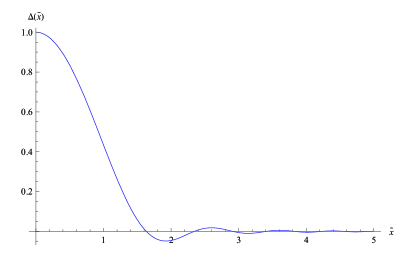
Figure 1: Solution of Eq.(27) for the Q2D conductor (3) in the parallel magnetic field (4) is shown. We pay attention to the fact that the solution is not of the Gaussian form, moreover it changes its sign several times with changing variable $\tilde{x}$.

Here, we consider the perpendicular upper critical magnetic field of the Q2D superconductor (3). Therefore, in this case, we choose magnetic field and vector potential in the the following form:

$${\bf H}=(0,0,H),\ \ \ {\bf H}=(0,Hx,0).$$ (29)

Using exactly the same steps and procedures as before for the parallel field, it is possible to obtain for the perpendicular field the following linearized Gor’kov’s equation [2,12] for non-uniform superconductivity:

$$\Delta(x)=g\biggl{<}\int^{\infty}_{d}\frac{2\pi Tdz}{v_{F}\sinh\biggl{(}\frac{2\pi Tz}{v_{F}}\biggl{)}}\cos\biggl{[}\frac{2\mu_{B}Hz}{v_{F}}\biggl{]}$$

$$\times\cos\biggl{\{}\frac{eH}{c}[z\sin\alpha(2x+z\cos\alpha)]\biggl{\}}\ \Delta(x+z\cos\alpha)\biggl{>}_{\alpha}.$$ (30)

Then, by means of the same method, as for the parallel magnetic field described in detail above, we obtain the similar GL equation in the perpendicular magnetic field (29):

$$-\xi^{2}_{\parallel}\frac{d^{2}\Delta(x)}{dx^{2}}+\biggl{(}\frac{2\pi H}{\phi_{0}}\biggl{)}^{2}\xi^{2}_{\parallel}x^{2}\Delta(x)-\tau\Delta(x)=0.$$ (31)

Analytic solution of the Eq.(31) results in the following formula for the GL slope of the perpendicular upper critical magnetic field:

$$H^{\perp}_{c2}=\tau\biggl{(}\frac{\phi_{0}}{2\pi\xi^{2}_{\parallel}}\biggl{)}=\tau\biggl{[}\frac{16\pi^{2}cT^{2}_{c}}{7\zeta(3)ev_{F}^{2}}\biggl{]}.$$ (32)

Repeating analogous analysis, as for the parallel magnetic field, we can write equation to determine the perpendicular upper critical magnetic field in the form:

$$\Delta(x)=g\biggl{<}\int^{\infty}_{d}\ \frac{dz}{z}\ \cos\biggl{\{}\frac{eH}{c}[z\sin\alpha(2x+z\cos\alpha)]\biggl{\}}$$

$$\times\Delta(x+z\cos\alpha)\biggl{>}_{\alpha},$$ (33)

which after introducing new variables,

$$\tilde{z}=\sqrt{\frac{eH}{c}}z,\ \ \ \tilde{x}=\sqrt{\frac{eH}{c}}x,$$ (34)

reduces to

$$\Delta(\tilde{x})=g\biggl{<}\int^{\infty}_{\sqrt{\frac{eH}{c}}d}\ \frac{d\tilde{z}}{\tilde{z}}\ \cos[\tilde{z}\sin\alpha(2\tilde{x}+\tilde{z}\cos\alpha)]$$

$$\times\Delta(\tilde{x}+\tilde{z}\cos\alpha)\biggl{>}_{\alpha}.$$ (35)

It is possible to prove that $\Delta(\tilde{x})=\exp(-\tilde{x}^{2})$ is the solution of Eq.(35) which gives the following value of the perpendicular upper critical magnetic field:

$$H^{\perp}_{c2}(0)\approx 0.59\biggl{[}\frac{16\pi^{2}cT^{2}_{c}}{7\zeta(3)ev_{F}^{2}}\biggl{]}=0.59\ |dH_{c2}^{\perp}/dT|_{T_{c}}T_{c}\ .$$ (36)

Let us discuss the possible applicability of the derived above Eqs.(28) and (36), which predict an increase of the Q2D anisotropy, $\gamma(T)=\biggl{[}\frac{H^{\parallel}_{c2}(T)}{H^{\perp}_{c2}(T)}\biggl{]}$, with decreasing temperature:

$$\lim_{T\rightarrow 0}\gamma(T)=\lim_{T\rightarrow 0}\biggl{[}\frac{H^{\parallel}_{c2}(T)}{H^{\perp}_{c2}(T)}\biggl{]}=1.27\lim_{T\rightarrow T_{c}}\gamma(T).$$ (37)

Note that, first of all, in the Letter, we consider the case of a clean Q2D superconductor, which is opposite to the so-called Lawrence-Doniach model [14,15]. Therefore, in our case, $\xi_{\perp}\gg c^{*}$ [see Eqs.(3) and (22)]. Secondly, the calculated orbital effect is supposed to be stronger than the Pauli spin-splitting effects [16-18] in a magnetic field and, thus, there are no conditions for the appearance of the Fulde-Ferrell-Larkin-Ovchinnikov phase [18-20]. We pay attention that there exists important high-temperature superconductor, $MgB_{2}$, where the above discussed conditions are fulfilled (see, for example, Refs. [21,22]) and where the above mentioned increase of $\gamma(T)$ is experimentally observed [5,6]. Our point of view is that this phenomena in $MgB_{2}$ is partially due to the effect, suggested in this Letter, and partially - due to the many-band effects [6,23,24], suggested for its explanation earlier.

In conclusion, we stress that all calculations for a Q2D superconductor in a magnetic field have been performed in the framework of the Fermi liquid theory [1]. In Q2D case, it is always possible to do, unlike Q1D one [25].

^∗Also at: L.D. Landau Institute for Theoretical Physics, RAS, 2 Kosygina Street, Moscow 117334, Russia.

References

• (1) See, for example, book A.A. Abrikosov, Fundamentals of Theory of Metals (Elsevier Science, Amsterdam, 1988).
• (2) L.P. Gor’kov, Sov. Phys. JETP, 37(10), 42 (1960).
• (3) N.R. Werthamer, E. Helfand, and P.C. Hohenberg, Phys. Rev. 147295 (1966).
• (4) L.P. Gor’kov and T.K. Melik-Barkhudarov, ZhETF, 45, 1493 (1964) [Sov. Phys. JETP, 18, 1031 (1964)].
• (5) V.G. Kogan and S.L. Bud’ko, Physica C 385, 131 (2003).
• (6) See, for example, review V.G. Kogan and R. Prozorov, Rep. Prog. Phys. 75, 114502 (2012).
• (7) See, for example, Takafumi Kita, Phys. Rev. B 68, 184503 (2003).
• (8) A.G. Lebed, JETP Lett. 44, 114 (1986) [Pis’ma Zh. Eksp. Teor. Fiz. 44, 89 (1986)].
• (9) N. Dupuis, G. Montambaux, and C.A.R. Sa de Melo, Phys. Rev. Lett. 70, 2613 (1993).
• (10) A.G. Lebed and K. Yamaji, Phys. Rev. Lett. 80, 2697 (1998).
• (11) L.P. Gor’kov and A.G. Lebed, J. Phys. (Paris) Lett. 45, L433 (1984).
• (12) A.A. Abrikosov, L.P. Gor’kov, and I.E. Dzyaloshinskii, Methods of Quantum Field Theory in Statistical Mechanics (Dover, New York, 1963).
• (13) I.S. Gradshteyn and I.M. Ryzhik, Table of Integrals, Series, and Products (6-th edition, Academic Press, London, United Kingdom, 2000).
• (14) L.N. Bulaevskii and A.A. Guseinov, Pis’ma Zh. Eksp. Teor. Fiz. 19, 742 (1974) [JETP Lett. 19, 382 (1974)].
• (15) R.A. Klemm, A. Luther, and M.R. Beasley, Phys. Rev. B 12, 877 (1975).
• (16) A.M. Clogston, Phys. Rev. Lett. 9, 266 (1962).
• (17) B.S. Chandrasekhar, Appl. Phys. Lett. 1, 7 (1962).
• (18) See, for example, A.G. Lebed, Phys. Rev. B 97, 144504 (2018).
• (19) P. Fulde and R.A. Ferrell, Phys. Rev. 135, A550 (1964).
• (20) A.I. Larkin and Yu.N. Ovchinnikov, Zh. Eksp. Teor. Fiz. 47, 1136 (1964) [Sov. Phys. JETP, 20, 762(1965)].
• (21) M.R. Eskildsen, M. Kugler, G. Levy, S. Tanaka, J. Jun, S.M. Kazakov, J. Karpinski, and O. Fischer, Physica C 385, 169 (2003).
• (22) J.C. Loudon, S. Yazdi, T.Kasama, N.D. Zhigadlo, and J. Karpinski, Phys. Rev. B 91, 054505 (2015).
• (23) P. Miranovic, K. Machida and V.G. Kogan, J. Phys. Soc. Jpn 72, 221 (2003).
• (24) T. Dahm and N. Schopoll, Phys. Rev. Lett. 91, 017001 (2003).
• (25) A.G. Lebed, Pis ma v ZhETF, 106, 491 (2017) [JETP Lett., 106, 509 (2017)].