Finite-Time Analysis of Round-Robin Kullback-Leibler Upper Confidence Bounds for Optimal Adaptive Allocation with Multiple Plays and Markovian Rewards

Abstract

We study an extension of the classic stochastic multi-armed bandit problem which involves multiple plays and Markovian rewards in the rested bandits setting. In order to tackle this problem we consider an adaptive allocation rule which at each stage combines the information from the sample means of all the arms, with the Kullback-Leibler upper confidence bound of a single arm which is selected in round-robin way. For rewards generated from a one-parameter exponential family of Markov chains, we provide a finite-time upper bound for the regret incurred from this adaptive allocation rule, which reveals the logarithmic dependence of the regret on the time horizon, and which is asymptotically optimal. For our analysis we devise several concentration results for Markov chains, including a maximal inequality for Markov chains, that may be of interest in their own right. As a byproduct of our analysis we also establish asymptotically optimal, finite-time guarantees for the case of multiple plays, and i.i.d. rewards drawn from a one-parameter exponential family of probability densities. Additionally, we provide simulation results that illustrate that calculating Kullback-Leibler upper confidence bounds in a round-robin way, is significantly more efficient than calculating them for every arm at each round, and that the expected regrets of those two approaches behave similarly.

1 Introduction

In this paper we study a generalization of the stochastic multi-armed bandit problem, where there are $K$ independent arms, and each arm $a\in[K]=\{1,\ldots,K\}$ is associated with a parameter $\theta_{a}\in{{\mathbb{R}}}$, and modeled as a discrete time stochastic process governed by the probability law $\operatorname{\mathbb{P}}_{\theta_{a}}$. A time horizon $T$ is prescribed, and at each round $t\in[T]=\{1,\ldots,T\}$ we select $M$ arms, where $1\leq M\leq K$, without any prior knowledge of the statistics of the underlying stochastic processes. The $M$ stochastic processes that correspond to the selected arms evolve by one time step, and we observe this evolution through a reward function, while the stochastic processes for the rest of the arms stay frozen, i.e. we consider the rested bandits setting. Our goal is to select arms in such a way so as to make the cumulative reward over the whole time horizon $T$ as large as possible. For this task we are faced with an exploitation versus exploration dilemma. At each round we need to decide whether we are going to exploit the best $M$ arms according to the information that we have gathered so far, or we are going to explore some other arms which do not seem to be so rewarding, just in case that the rewards we have observed so far deviate significantly from the expected rewards. The answer to this dilemma is usually coming by calculating indices for the arms and ranking them according to those indices, which should incorporate both information on how good an arm seems to be as well as on how many times it has been played so far. Here we take an alternative approach where instead of calculating the indices for all the arms at each round, we just calculate the index for a single arm in a round-robin way.

1.1 Contributions

1. We first consider the case that the $K$ stochastic processes are irreducible Markov chains, coming from a one-parameter exponential family of Markov chains. The objective is to play as much as possible the $M$ arms with the largest stationary means, although we have no prior information about the statistics of the $K$ Markov chains. The difference of the best possible expected rewards coming from those $M$ best arms and the expected reward coming from the arms that we played is the regret that we incur. To minimize the regret we consider an index based adaptive allocation rule, Algorithm 1, which is based on sample means and Kullback-Leibler upper confidence bounds for the stationary expected rewards using the Kullback-Leibler divergence rate. We provide a finite-time analysis, Theorem 1, for this KL-UCB adaptive allocation rule which shows that the regret depends logarithmically on the time horizon $T$, and matches exactly the asymptotic lower bound, Corollary 1.

2. In order to make the finite-time guarantee possible we devise several deviation lemmata for Markov chains. An exponential martingale for Markov chains is proven, Lemma 1, which leads to a maximal inequality for Markov chains, Lemma 2. In the literature there are several approaches that use martingale techniques either to derive Hoeffding inequalities for Markov chains Glynn and Ormoneit, (2002); Moulos, (2020), or more generally to study concentration of measure for Markov chains Marton, 1996a ; Marton, 1996b ; Marton, (1998); Samson, (2000); Marton, (2003); Chazottes et al., (2007); Kontorovich and Ramanan, (2008); Paulin, (2015). Nonetheless, they’re all based either on Dynkin’s martingale or on Doob’s martingale, combined with coupling ideas, and there is no evidence that they can lead to maximal inequalities. Moreover, a Chernoff bound for Markov chains is devised, Lemma 3, and its relation with the work of Moulos and Anantharam, (2019) is discussed in Remark 5.

3. We then consider the case that the $K$ stochastic processes are i.i.d. processes, each corresponding to a density coming from a one-parameter exponential family of densities. We establish, Theorem 2, that Algorithm 1 still enjoys the same finite-time regret guarantees, which are asymptotically optimal. The case where Theorem 2 follows directly from Theorem 1 is discussed in Remark 3. The setting of single plays is studied in Cappé et al., (2013), but with a much more computationally intense adaptive allocation rule.

4. In Section 6 we provide simulation results illustrating the fact that round-robin KL-UCB adaptive allocation rules are much more computationally efficient than KL-UCB adaptive allocation rules, and similarly round-robin UCB adaptive allocation rules are more computationally efficient than UCB adaptive allocation rules, while the expected regrets, in each family of algorithms, behave in a similar way. This brings to light round-robin schemes as an appealing practical alternative to the mainstream schemes that calculate indices for all the arms at each round.

1.2 Motivation

Multi-armed bandits provide a simple abstract statistical model that can be applied to study real world problems such as clinical trials, ad placement, gambling, adaptive routing, resource allocation in computer systems etc. We refer the interested reader to the survey of Bubeck and Cesa-Bianchi, (2012) for more context, and to the recent books of Lattimore and Szepesvári, (2019); Slivkins, (2019). The need for multiple plays can be understood in the setting of resource allocation. Scheduling jobs to a single CPU is an instance of the multi-armed bandit problem with a single play at each round, where the arms correspond to the jobs. If there are multiple CPUs we get an instance of the multi-armed bandit problem with multiple plays. The need of a richer model which allows the presence of Markovian dependence is illustrated in the context of gambling, where the arms correspond to slot-machines. It is reasonable to try to model the assertion that if a slot-machine produced a high reward the $n$-th time played, then it is very likely that it will produce a much lower reward the $(n+1)$-th time played, simply because the casino may decide to change the reward distribution to a much stingier one if a big reward was just produced. This assertion requires, the reward distributions to depend on the previous outcome, which is precisely captured by the Markovian reward model. Moreover, we anticipate this to be an important problem attempting to bridge classical stochastic bandits, controlled Markov chains (MDPs), and non-stationary bandits.

1.3 Related Work

The cornerstone of the multi-armed bandits literature is the pioneering work of Lai and Robbins, (1985), which studies the problem for the case of i.i.d. rewards and single plays. Lai and Robbins, (1985) introduce the change of measure argument to derive a lower bound for the problem, as well as round robin adaptive allocation rules based on upper confidence bounds which are proven to be asymptotically optimal. Anantharam et al., 1987a extend the results of Lai and Robbins, (1985) to the case of i.i.d. rewards and multiple plays, while Agrawal, (1995) considers index based allocation rules which are only based on sample means and are computationally simpler, although they may not be asymptotically optimal. The work of Agrawal, (1995) inspired the first finite-time analysis for the adaptive allocation rule called UCB by Auer et al., (2002), which is though asymptotically suboptimal. The works of Cappé et al., (2013); Garivier and Cappé, (2011); Maillard et al., (2011) bridge this gap by providing the KL-UCB adaptive allocation rule, with finite-time guarantees which are asymptotically optimal. Additionally, Komiyama et al., (2015) study a Thompson sampling algorithm for multiple plays and binary rewards, and they establish a finite-time analysis which is asymptotically optimal. Here we close the problem of multiple plays and rewards coming from an exponential family of probability densities by showing finite-time guarantees which are asymptotically optimal, via adaptive allocation rules which are much more efficiently computable than their precursors.

The study of Markovian rewards and multiple plays in the rested setting, is initiated in the work of Anantharam et al., 1987b . They report an asymptotic lower bound, as well as a round robin upper confidence bound adaptive allocation rule which is proven to be asymptotically optimal. However, it is unclear if the statistics that they use in order to derive the upper confidence bounds, in their Theorem 4.1, can be recursively computed, and the practical applicability of their results is therefore questionable. In addition, they don’t provide any finite-time analysis, and they use a different type of assumption on their one-parameter family of Markov chains. In particular, they assume that their one-parameter family of transition probability matrices is log-concave in the parameter, equation (4.1) in Anantharam et al., 1987b , while we assume that it is a one-parameter exponential family of transition probability matrices. Tekin and Liu, (2010, 2012) extend the UCB adaptive allocation rule of Auer et al., (2002), to the case of Markovian rewards and multiple plays. They provide a finite-time analysis, but their regret bounds are suboptimal. Moreover they impose a different type of assumption on their configuration of Markov chains. They assume that the transition probability matrices are reversible, so that they can apply Hoeffding bounds for Markov chains from Gillman, (1993); Lezaud, (1998). In a recent work Moulos, (2020) developed a Hoeffding bound for Markov chains, which does not assume any conditions other than irreducibility, and using this he extended the analysis of UCB to an even broader class of Markov chains. One of our main contributions is to bridge this gap and provide a KL-UCB adaptive allocation rule, with a finite-time guarantee which is asymptotically optimal. In a different line of work Ortner et al., (2012); Tekin and Liu, (2012) consider the restless bandits Markovian reward model, in which the state of each arm evolves according to a Markov chain independently of the player’s action. Thus in the restless setting the state that we next observe is now dependent on the amount of time that elapses between two plays of the same arm.

2 Problem Formulation

2.1 One-Parameter Family of Markov Chains

We consider a one-parameter family of irreducible Markov chains on a finite state space $S$. Each member of the family is indexed by a parameter $\theta\in{{\mathbb{R}}}$, and is characterized by an initial distribution $q_{\theta}=[q_{\theta}(x)]_{x\in S}$, and an irreducible transition probability matrix $P_{\theta}=[P_{\theta}(x,y)]_{x,y\in S}$, which give rise to a probability law $\operatorname{\mathbb{P}}_{\theta}$. There are $K\geq 2$ arms, with overall parameter configuration ${\boldsymbol{\theta}}=(\theta_{1},\ldots,\theta_{K})\in{{\mathbb{R}}}^{K}$, and each arm $a\in[K]=\{1,\ldots,K\}$ evolves internally as the Markov chain with parameter $\theta_{a}$ which we denote by $\{X_{n}^{a}\}_{n\in{{\mathbb{Z}_{\geq 0}}}}$. There is a common noncostant real-valued reward function on the state space $f:S\to{{\mathbb{R}}}$, and successive plays of arm $a$ result in observing samples from the stochastic process $\{Y_{n}^{a}\}_{n\in{{\mathbb{Z}_{\geq 0}}}}$, where $Y_{n}^{a}=f(X_{n}^{a})$. In other words, the distribution of the rewards coming from arm $a$ is a function of the Markov chain with parameter $\theta_{a}$, and thus it can have more complicated dependencies. As a special case, if we pick the reward function $f$ to be injective, then the distribution of the rewards is Markovian.

For $\theta\in{{\mathbb{R}}}$, due to irreducibility, there exists a unique stationary distribution for the transition probability matrix $P_{\theta}$ which we denote with $\pi_{\theta}=[\pi_{\theta}(x)]_{x\in S}$. Furthermore, let $\mu(\theta)=\sum_{x\in S}f(x)\pi_{\theta}(x)$ be the stationary mean reward corresponding to the Markov chain parametrized by $\theta$. Without loss of generality we may assume that the $K$ arms are ordered so that,

$$\mu(\theta_{1})\geq\ldots\geq\mu(\theta_{N})>\mu(\theta_{N+1})\ldots=\mu(\theta_{M})=\ldots=\mu(\theta_{L})>\mu(\theta_{L+1})\geq\ldots\geq\mu(\theta_{K}),$$

for some $N\in\{0,\ldots,M-1\}$ and $L\in\{M,\ldots,K\}$, where $N=0$ means that $\mu(\theta_{1})=\ldots=\mu(\theta_{M}),~{}L=K$ means that $\mu(\theta_{M})=\ldots=\mu(\theta_{K})$, and we set $\mu(\theta_{0})=\infty$ and $\mu(\theta_{K+1})=-\infty$.

2.2 Regret Minimization

We fix a time horizon $T$, and at each round $t\in[T]=\{1,\ldots,T\}$ we play a set $\phi_{t}$ of $M$ distinct arms, where $1\leq M\leq K$ is the same through out the rounds, and we observe rewards $\{Z_{t}^{a}\}_{a\in[K]}$ given by,

$$Z_{t}^{a}=\begin{cases}Y_{N_{a}(t)}^{a},&\text{if}~{}a\in\phi_{t}\\ 0,&\text{if}~{}a\not\in\phi_{t},\end{cases}$$

where $N^{a}(t)=\sum_{s=1}^{t}I\{a\in\phi_{s}\}$ is the number of times we played arm $a$ up to time $t$. Using the stopping times $\tau_{n}^{a}=\inf\{t\geq 1:N^{a}(t)=n\}$, we can also reconstruct the $\{Y_{n}^{a}\}_{n\in{{\mathbb{Z}_{>0}}}}$ process, from the observed $\{Z_{t}^{a}\}_{t\in{{\mathbb{Z}_{>0}}}}$ process, via the identity $Y_{n}^{a}=Z_{\tau_{n}^{a}}^{a}$. Our play $\phi_{t}$ is based on the information that we have accumulated so far. In other words, the event $\{\phi_{t}=A\}$, for $A\subseteq[K]$ with $|A|=M$, belongs to the $\sigma$-field generated by $\phi_{1},\{Z_{1}^{a}\}_{a\in[K]},\ldots,\phi_{t-1},\{Z_{t-1}^{a}\}_{a\in[K]}$. We call the sequence ${\boldsymbol{\phi}}=\{\phi_{t}\}_{t\in{{\mathbb{Z}}}_{>0}}$ of our plays an adaptive allocation rule. Our goal is to come up with an adaptive allocation rule ${\boldsymbol{\phi}}$, that achieves the greatest possible expected value for the sum of the rewards,

$$S_{T}=\sum_{t=1}^{T}\sum_{a\in[K]}Z_{t}^{a}=\sum_{a\in[K]}\sum_{n=1}^{N^{a}(T)}Y_{n}^{a},$$

which is equivalent to minimizing the expected regret,

$$R_{\boldsymbol{\theta}}^{\boldsymbol{\phi}}(T)=T\sum_{a=1}^{M}\mu(\theta_{a})-\operatorname{\mathbb{E}}_{\boldsymbol{\theta}}^{\boldsymbol{\phi}}[S_{T}].$$ (1)

2.3 Asymptotic Lower Bound

A quantity that naturally arises in the study of regret minimization for Markovian bandits is the Kullback-Leibler divergence rate between two Markov chains, which is a generalization of the usual Kullback-Leibler divergence between two probability distributions. We denote by ${D\left({\theta}\;\middle\|\;{\lambda}\right)}$ the Kullback-Leibler divergence rate between the Markov chain with parameter $\theta$ and the Markov chain with parameter $\lambda$, which is given by,

$${D\left({\theta}\;\middle\|\;{\lambda}\right)}=\sum_{x,y\in S}\log\frac{P_{\theta}(x,y)}{P_{\lambda}(x,y)}\pi_{\theta}(x)P_{\theta}(x,y),$$ (2)

where we use the standard notational conventions $\log 0=\infty,~{}\log\frac{\alpha}{0}=\infty~{}\text{if}~{}\alpha>0$, and $0\log 0=0\log\frac{0}{0}=0$. Indeed note that, if $P_{\theta}(x,\cdot)=p_{\theta}(\cdot)$ and $P_{\lambda}(x,\cdot)=p_{\lambda}(\cdot)$, for all $x\in S$, i.e. in the special case that the Markov chains correspond to IID processes, then the Kullback-Leibler divergence rate ${D\left({\theta}\;\middle\|\;{\lambda}\right)}$ is equal to the Kullback-Leibler divergence ${D\left({p_{\theta}}\;\middle\|\;{p_{\lambda}}\right)}$ between $p_{\theta}$ and $p_{\lambda}$,

$${D\left({\theta}\;\middle\|\;{\lambda}\right)}=\sum_{x,y\in S}\log\frac{p_{\theta}(y)}{p_{\lambda}(y)}p_{\theta}(x)p_{\theta}(y)=\sum_{y\in S}\log\frac{p_{\theta}(y)}{p_{\theta}(y)}p_{\theta}(y)={D\left({p_{\theta}}\;\middle\|\;{p_{\lambda}}\right)}.$$

Under some regularity assumptions on the one-parameter family of Markov chains, Anantharam et al., 1987b in their Theorem 3.1 are able to establish the following asymptotic lower bound on the expected regret for any adaptive allocation rule ${\boldsymbol{\phi}}$ which is uniformly good across all parameter configurations,

$$\liminf_{T\to\infty}\frac{R_{\boldsymbol{\theta}}^{\boldsymbol{\phi}}(T)}{\log T}\geq\sum_{b=L+1}^{K}\frac{\mu(\theta_{M})-\mu(\theta_{b})}{{D\left({\theta_{b}}\;\middle\|\;{\theta_{M}}\right)}}.$$ (3)

A further discussion of this lower bound, as well as an alternative derivation can be found in Appendix D,

The main goal of this work is to derive a finite time analysis for an adaptive allocation rule which is based on Kullback-Leibler divergence rate indices, that is asymptotically optimal. We do so for the one-parameter exponential family of Markov chains, which forms a generalization of the classic one-parameter exponential family generated by a probability distribution with finite support.

2.4 One-Parameter Exponential Family Of Markov Chains

Let $S$ be a finite state space, $f:S\to{{\mathbb{R}}}$ be a nonconstant reward function on the state space, and $P$ an irreducible transition probability matrix on $S$, with associated stationary distribution $\pi$. $P$ will serve as the generator stochastic matrix of the family. Let $\mu(0)=\sum_{x\in S}f(x)\pi(x)$ be the stationary mean of the Markov chain induced by $P$ when $f$ is applied. By tilting exponentially the transitions of $P$ we are able to construct new transition matrices that realize a whole range of stationary means around $\mu(0)$ and form the exponential family of stochastic matrices. Let $\theta\in{{\mathbb{R}}}$, and consider the matrix $\tilde{P}_{\theta}(x,y)=P(x,y)e^{\theta f(y)}$. Denote by $\rho(\theta)$ its spectral radius. According to the Perron-Frobenius theory, see Theorem 8.4.4 in the book of Horn and Johnson, (2013), $\rho(\theta)$ is a simple eigenvalue of $\tilde{P}_{\theta}$, called the Perron-Frobenius eigenvalue, and we can associate to it unique left $u_{\theta}$ and right $v_{\theta}$ eigenvectors such that they are both positive, $\sum_{x\in S}u_{\theta}(x)=1$ and $\sum_{x\in S}u_{\theta}(x)v_{\theta}(x)=1$. Using them we define the member of the exponential family which corresponds to the natural parameter $\theta$ as,

$$P_{\theta}(x,y)=\frac{v_{\theta}(y)}{v_{\theta}(x)}\exp\left\{\theta f(y)-\Lambda(\theta)\right\}P(x,y),$$ (4)

where $\Lambda(\theta)=\log\rho(\theta)$ is the log-Perron-Frobenius eigenvalue. It can be easily seen that $P_{\theta}(x,y)$ is indeed a stochastic matrix, and its stationary distribution is given by $\pi_{\theta}(x)=u_{\theta}(x)v_{\theta}(x)$. The initial distribution $q_{\theta}$ associated to the parameter $\theta$, can be any distribution on $S$, since the KL-UCB adaptive allocation rule that we devise, and its guarantees, will be valid no matter the initial distributions.

Example 1 (Two-state chain).

Let $S=\{0,1\}$, and consider the transition probability matrix, $P$, representing two coin-flips, $\operatorname{Bernoulli}(p)$ when we’re in state $0$, and $\operatorname{Bernoulli}(q)$ when we’re in state $1$. We require that $P$ is irreducible, so $p\in(0,1]$ and $q\in[0,1)$.

$$P=\begin{bmatrix}1-p&p\\ 1-q&q\end{bmatrix}$$

The exponential family of transition probability matrices generated by $P$ and $f(x)=2x-1$ is given by,

$$P_{\theta}=\frac{1}{\rho(\theta)}\begin{bmatrix}(1-p)e^{-\theta}&\rho(\theta)-(1-p)e^{-\theta}\\ \rho(\theta)-qe^{\theta}&qe^{\theta}\end{bmatrix},$$

where,

$$\rho(\theta)=\frac{(1-p)e^{-\theta}+qe^{\theta}+\sqrt{((1-p)e^{-\theta}-qe^{\theta})^{2}+4p(1-q)}}{2}.$$

In the special case that $p=q$, we get back the typical exponential family of $\operatorname{Bernoulli}(p_{\theta})$ coin-flips, with

$$1-p_{\theta}=\frac{(1-p)e^{-\theta}}{(1-p)e^{-\theta}+pe^{\theta}}.$$

Exponential families of Markov chains date back to the work of Miller, (1961). For a short overview of one-parameter exponential families of Markov chains, as well as proofs of the following properties, we refer the reader to Section 2 in Moulos and Anantharam, (2019). The log-Perron-Frobenius eigenvalue $\Lambda(\theta)$ is a convex analytic function on the real numbers, and through its derivative, $\dot{\Lambda}(\theta)$, we obtain the stationary mean $\mu(\theta)$ of the Markov chain with transition matrix $P_{\theta}$ when $f$ is applied, i.e. $\dot{\Lambda}(\theta)=\mu(\theta)=\sum_{x\in S}f(x)\pi_{\theta}(x)$. When $\Lambda(\theta)$ is not the linear function $\theta\mapsto\mu(0)\theta$, the log-Perron-Frobenius eigenvalue, $\Lambda(\theta)$, is strictly convex and thus its derivative $\dot{\Lambda}(\theta)$ is strictly increasing, and it forms a bijection between the natural parameter space, ${{\mathbb{R}}}$, and the mean parameter space, ${\mathcal{M}}=\dot{\Lambda}({{\mathbb{R}}})$, which is a bounded open interval.

The Kullback-Leibler divergence rate from (2), when instantiated for the exponential family of Markov chains, can be expressed as,

$${D\left({\theta}\;\middle\|\;{\lambda}\right)}=\Lambda(\lambda)-\Lambda(\theta)-\dot{\Lambda}(\theta)(\lambda-\theta),$$

which is convex and differentiable over ${{\mathbb{R}}}\times{{\mathbb{R}}}$. Since $\dot{\Lambda}:{{\mathbb{R}}}\to{\mathcal{M}}$ forms a bijection from the natural parameter space, ${{\mathbb{R}}}$, to the mean parameter space, ${\mathcal{M}}$, with some abuse of notation we will write ${D\left({\mu}\;\middle\|\;{\nu}\right)}$ for ${D\left({\dot{\Lambda}^{-1}(\mu)}\;\middle\|\;{\dot{\Lambda}^{-1}(\nu)}\right)}$, where $\mu,\nu\in{\mathcal{M}}$. Furthermore, ${D\left({\cdot}\;\middle\|\;{\cdot}\right)}:{\mathcal{M}}\times{\mathcal{M}}\to{{\mathbb{R}}}_{\geq 0}$ can be extended continuously, to a function ${D\left({\cdot}\;\middle\|\;{\cdot}\right)}:\bar{{\mathcal{M}}}\times\bar{{\mathcal{M}}}\to{{\mathbb{R}}}_{\geq 0}\cup\{\infty\}$, where $\bar{{\mathcal{M}}}$ denotes the closure of ${\mathcal{M}}$. This can even further be extended to a convex function on ${{\mathbb{R}}}\times{{\mathbb{R}}}$, by setting ${D\left({\mu}\;\middle\|\;{\nu}\right)}=\infty$ if $\mu\not\in\bar{{\mathcal{M}}}$ or $\nu\not\in\bar{{\mathcal{M}}}$. For fixed $\nu\in{{\mathbb{R}}}$, the function $\mu\mapsto{D\left({\mu}\;\middle\|\;{\nu}\right)}$ is decreasing for $\mu\leq\nu$ and increasing for $\mu\geq\nu$. Similarly, for fixed $\mu\in{{\mathbb{R}}}$, the function $\nu\mapsto{D\left({\mu}\;\middle\|\;{\nu}\right)}$ is decreasing for $\nu\leq\mu$ and increasing for $\nu\geq\mu$.

3 A Maximal Inequality for Markov Chains

Here we present an exponential martingale for Markov chains, which in turn leads to a maximal inequality. For proofs, and a Chernoff bound for Markov chains we refer the interested reader to Appendix A.

Lemma 1 (Exponential martingale for Markov chains).

Let $\{X_{n}\}_{n\in{{\mathbb{Z}}}_{\geq 0}}$ be a Markov chain over the finite state space $S$ with an irreducible transition matrix $P$ and initial distribution $q$. Let $f:S\to{{\mathbb{R}}}$ be a nonconstant real-valued function on the state space. Fix $\theta\in{{\mathbb{R}}}$ and define,

$$M_{n}^{\theta}=\frac{v_{\theta}(X_{n})}{v_{\theta}(X_{0})}\exp\left\{\theta(f(X_{1})+\ldots+f(X_{n}))-n\Lambda(\theta)\right\}.$$ (5)

Then $\{M_{n}^{\theta}\}_{n\in{{\mathbb{Z}_{>0}}}}$ is a martingale with respect to the filtration $\{{\mathcal{F}}_{n}\}_{n\in{{\mathbb{Z}_{>0}}}}$, where ${\mathcal{F}}_{n}$ is the $\sigma$-field generated by $X_{0},\ldots,X_{n}$.

The following definition is the technical condition that we will require for our maximal inequality.

Definition 1 (Doeblin’s type of condition).

Let $P$ be a transition probability matrix on the finite state space $S$. For a nonempty set of states $A\subset S$, we say that $P$ is $A$-Doeblin if, the submatrix of $P$ with rows and columns in $A$ is irreducible, and for every $x\in S-A$ there exists $y\in A$ such that $P(x,y)>0$.

Example 1 (continued).

For this example $P$ being $\{0\}$-Doeblin means that $p,q\in[0,1)$, but already irreducibility imposed the constraints $p\in(0,1]$ and $q\in[0,1)$, hence the only additional constraint is $p\neq 1$.

Remark 1.

Our Definition 1 is inspired by the classic Doeblin’s Theorem, see Theorem 2.2.1 in Stroock, (2014). Doeblin’s Theorem states that, if the transition probability matrix $P$ satisfies Doeblin’s condition (namely there exists $\epsilon>0$, and a state $y\in S$ such that for all $x\in S$ we have $P(x,y)\geq\epsilon$), then $P$ has a unique stationary distribution $\pi$, and for all initial distributions $q$ we have geometric convergence to stationarity, i.e. $\|qP^{n}-\pi\|_{1}\leq 2(1-\epsilon)^{n}$. Doeblin’s condition, according to our Definition 1, corresponds to $P$ being $\{y\}$-Doeblin for some $y\in S$.

Lemma 2 (Maximal inequality for irreducible Markov chains satisfying Doeblin’s condition).

Let $\{X_{n}\}_{n\in{{\mathbb{Z}}}_{\geq 0}}$ be an irreducible Markov chain over the finite state space $S$ with transition matrix $P$, initial distribution $q$, and stationary distribution $\pi$. Let $f:S\to{{\mathbb{R}}}$ be a non-constant function on the state space. Denote by $\mu(0)=\sum_{x\in S}f(x)\pi(x)$ the stationary mean when $f$ is applied, and by $\bar{Y}_{n}=\frac{1}{n}\sum_{k=1}^{n}Y_{k}$ the empirical mean, where $Y_{k}=f(X_{k})$. Assume that $P$ is $\left(\operatorname*{arg\,min}_{x\in S}f(x)\right)$-Doeblin. Then for all $\epsilon>1$ we have

$$\operatorname{\mathbb{P}}\left(\bigcup_{k=1}^{n}\left\{\mu(0)\geq\bar{Y}_{k}~{}\text{and}~{}k{D\left({\bar{Y}_{k}}\;\middle\|\;{\mu(0)}\right)}\geq\epsilon\right\}\right)\leq C_{-}e\lceil\epsilon\log n\rceil e^{-\epsilon},$$

where $C_{-}=C_{-}(P,f)$ is a positive constant depending only on the transition probability matrix $P$ and the function $f$.

Remark 2.

If we only consider values of $\epsilon$ from a bounded subset of $(1,\infty)$, then we don’t need to assume that $P$ is $\left(\operatorname*{arg\,min}_{x\in S}f(x)\right)$-Doeblin, and the constant $C_{-}$ will further depend on this bounded subset. But in the analysis of the KL-UCB adaptive allocation rule we will need to consider values of $\epsilon$ that increase with the time horizon $T$, therefore we have to impose the assumption that $P$ is $\left(\operatorname*{arg\,min}_{x\in S}f(x)\right)$-Doeblin, so that $C_{-}$ has no dependencies on $\epsilon$.

i.i.d. versions of this maximal inequality have found applicability not only in multi-armed bandit problems, but also in the case of context tree estimation, Garivier and Leonardi, (2011), indicating that our Lemma 2 may be of interest for other applications as well.

4 The Round-Robin KL-UCB Adaptive Allocation Rule for Multiple Plays and Markovian Rewards

For each arm $a\in[K]$ we define the empirical mean at the global time $t$ as,

$$\bar{Y}_{a}(t)=(Y_{1}^{a}+\ldots+Y_{N_{a}(t)}^{a})/N_{a}(t),$$ (6)

and its local time counterpart as,

$$\bar{Y}_{n}^{a}=(Y_{1}^{a}+\ldots+Y_{n}^{a})/n,$$

with their link being $\bar{Y}_{n}^{a}=\bar{Y}_{a}(\tau_{n}^{a})$, where $\tau_{n}^{a}=\inf\{t\geq 1:N_{a}(t)=n\}$. At each round $t$ we calculate a single upper confidence bound index,

$$U_{a}(t)=\sup\left\{\mu\in{\mathcal{M}}:{D\left({\bar{Y}_{a}(t)}\;\middle\|\;{\mu}\right)}\leq\frac{g(t)}{N_{a}(t)}\right\},$$ (7)

where $g(t)$ is an increasing function, and we denote its local time version by,

$$U_{n}^{a}(t)=\sup\left\{\mu\in{\mathcal{M}}:{D\left({\bar{Y}_{n}^{a}}\;\middle\|\;{\mu}\right)}\leq\frac{g(t)}{n}\right\}.$$

Note that $U_{a}(t)$ is efficiently computable via a bisection method due to the monotonicity of ${D\left({\bar{Y}_{a}(t)}\;\middle\|\;{\cdot}\right)}$. It is straightforward to check, using the definition of $U_{n}^{a}(t)$, the following two relations,

$$\bar{Y}_{n}^{a}\leq U_{n}^{a}(t)~{}\text{for all}~{}n\leq t,$$ (8)

$$U_{n}^{a}(t)~{}\text{is increasing in}~{}t\geq n~{}\text{for fixed}~{}n.$$ (9)

Furthermore, in Appendix B we study the concentration properties of those upper confidence indices and of the sample means, using the concentration results for Markov chains from Section 3. The idea of calculating indices in a round robin way, dates back to the seminal work of Lai and Robbins, (1985). Here we exploit this idea, which seems to have been forgotten over time in favor of algorithms that calculate indices for all the arms at each round, and we augment it with the usage of the upper confidence bounds in (7), which are efficiently computable, see Section 6 for simulation results, as opposed to the statistics in Theorem 4.1 from Anantharam et al., 1987b . Moreover, this combination of a round-robin scheme and the indices in (7) is amenable to a finite-time analysis, see Appendix C.

Parameters: number of arms $K\geq 2$, time horizon $T\geq K$, number of plays $1\leq M\leq K$,

KL divergence rate function ${D\left({\cdot}\;\middle\|\;{\cdot}\right)}:\bar{{\mathcal{M}}}\times\bar{{\mathcal{M}}}\to{{\mathbb{R}}}_{\geq 0}$, increasing function $g:{{\mathbb{Z}_{>0}}}\to{{\mathbb{R}}}$, parameter $\delta\in(0,1/K)$ ;

Initializaton: In the first $K$ rounds pull each arm $M$ times and set $\bar{Y}_{a}(K)=(Y_{1}^{a}+\ldots+Y_{M}^{a})/M$, for $a=1,\ldots,K$ ;

for $t=K,\ldots,T-1$ do

       Let $W_{t}=\{a\in[K]:N_{a}(t)\geq\lceil\delta t\rceil\}$;

Pick any subset of arms $L_{t}\subseteq W_{t}$ such that:

•  

  $|L_{t}|=M$;

 

and $\displaystyle\min_{a\in L_{t}}\bar{Y}_{a}(t)\geq\sup_{b\in W_{t}-L_{t}}\bar{Y}_{b}(t)$;

       Let $b\equiv t+1\pmod{K}$, with $b\in[K]$;

       Let $\displaystyle U_{b}(t)=\sup\left\{\mu\in{\mathcal{M}}:{D\left({\bar{Y}_{b}(t)}\;\middle\|\;{\mu}\right)}\leq\frac{g(t)}{N_{b}(t)}\right\}$;

       if $b\in L_{t}$ or $\displaystyle\min_{a\in L_{t}}\bar{Y}_{a}(t)\geq U_{b}(t)$ then

            Pull the $M$ arms in $\phi_{t+1}=L_{t}$;

      else

            Pick any $\displaystyle a\in\operatorname*{arg\,min}_{a\in L_{t}}\bar{Y}_{a}(t)$;

             Pull the $M$ arms in $\phi_{t+1}=(L_{t}\setminus\{a\})\cup\{b\}$;

            

       end if

      

end for

Algorithm 1 The round-robin KL-UCB adaptive allocation rule.

Proposition 1.

For each $t\geq K$ we have that $|W_{t}|\geq M$, and so Algorithm 1 is well defined.

Theorem 1 (Markovian rewards and multiple plays: finite-time guarantees).

Let $P$ be an irreducible transition probability matrix on the finite state space $S$, and $f:S\to{{\mathbb{R}}}$ be a real-valued reward function, such that $P$ is $\left(\operatorname*{arg\,min}_{x\in S}f(x)\right)$-Doeblin. Assume that the $K$ arms correspond to the parameter configuration ${\boldsymbol{\theta}}\in{{\mathbb{R}}^{K}}$ of the exponential family of Markov chains, as described in Equation 4. Without loss of generality assume that the $K$ arms are ordered so that,

$$\mu(\theta_{1})\geq\ldots\geq\mu(\theta_{N})>\mu(\theta_{N+1})\ldots=\mu(\theta_{M})=\ldots=\mu(\theta_{L})>\mu(\theta_{L+1})\geq\ldots\geq\mu(\theta_{K}).$$

Fix $\epsilon\in\left(0,\min(\mu(\theta_{N})-\mu(\theta_{M}),\mu(\theta_{M})-\mu(\theta_{L+1}))\right)$. The KL-UCB adaptive allocation rule for Markovian rewards and multiple plays, Algorithm 1, with the choice $g(t)=\log t+3\log\log t$, enjoys the following finite-time upper bound on the regret,

$$R_{\boldsymbol{\theta}}^{\boldsymbol{\phi}}(T)\leq\sum_{b=L+1}^{K}\frac{\mu(\theta_{M})-\mu(\theta_{b})}{{D\left({\mu(\theta_{b})}\;\middle\|\;{\mu(\theta_{M})-\epsilon}\right)}}\log T+c_{1}\sqrt{\log T}+c_{2}\log\log T+c_{3}\sqrt{\log\log T}+c_{4},$$

where $c_{1},c_{2},c_{3},c_{4}$ are constants with respect to $T$, which are given more explicitly in the analysis.

Corollary 1 (Asymptotic optimality).

In the context of Theorem 1 the KL-UCB adaptive allocation rule, Algorithm 1, is asymptotically optimal, and,

$$\lim_{T\to\infty}\frac{R_{\boldsymbol{\theta}}^{\boldsymbol{\phi}}(T)}{\log T}=\sum_{b=L+1}^{K}\frac{\mu(\theta_{M})-\mu(\theta_{b})}{{D\left({\mu(\theta_{b})}\;\middle\|\;{\mu(\theta_{M})}\right)}}.$$

5 The Round-Robin KL-UCB Adaptive Allocation Rule for Multiple Plays and i.i.d. Rewards

As a byproduct of our work in Section 4 we further obtain a finite-time regret bound, which is asymptotically optimal, for the case of multiple plays and i.i.d. rewards, from an exponential family of probability densities.

We first review the notion of an exponential family of probability densities, for which the standard reference is Brown, (1986). Let $(X,{\mathcal{X}},\rho)$ be a probability space. A one-parameter exponential family is a family of probability densities $\{p_{\theta}:\theta\in\Theta\}$ with respect to the measure $\rho$ on $X$, of the form,

$$p_{\theta}(x)=\exp\{\theta f(x)-\Lambda(\theta)\}h(x),$$ (10)

where $f:X\to{{\mathbb{R}}}$ is called the sufficient statistic, is ${\mathcal{X}}$-measurable, and there is no $c\in{{\mathbb{R}}}$ such that $f(x)\stackrel{{\scriptstyle\rho-a.s.}}{{=}}c,~{}h:X\to{{\mathbb{R}}_{\geq 0}}$ is called the carrier density, and is a density with respect to $\rho$, and $\Lambda$ is called the log-Moment-Generating-Function and is given by $\Lambda(\theta)=\log\int_{X}e^{\theta f(x)}h(x)\rho(dx)$, which is finite for $\theta$ in the natural parameter space $\Theta=\{\theta\in{{\mathbb{R}}}:\int_{X}e^{\theta f(x)}h(x)\rho(dx)<\infty\}$. The log-MGF, $\Lambda(\theta)$, is strictly convex and its derivative forms a bijection between the natural parameters, $\theta$, and the mean parameters, $\mu(\theta)=\int_{X}f(x)p_{\theta}(x)\rho(dx)$. The Kullback-Leibler divergence between $p_{\theta}$ and $p_{\lambda}$, for $\theta,\lambda\in\Theta$, can be written as ${D\left({\theta}\;\middle\|\;{\lambda}\right)}=\Lambda(\lambda)-\Lambda(\theta)-\dot{\Lambda}(\theta)(\lambda-\theta)$.

For this section, each arm $a\in[K]$ with parameter $\theta_{a}$ corresponds to the i.i.d. process $\{X_{n}^{a}\}_{n\in{{\mathbb{Z}_{>0}}}}$, where each $X_{n}^{a}$ has density $p_{\theta_{a}}$ with respect to $\rho$, which gives rise to the i.i.d. reward process $\{Y_{n}^{a}\}_{n\in{{\mathbb{Z}_{>0}}}}$, with $Y_{n}^{a}=f(X_{n}^{a})$.

Remark 3.

When there is a finite set $S\in{\mathcal{X}}$ such that $\rho(S)=1$, then the exponential family of probability densities in Equation 10, is just a special case of the exponential family of Markov chains in Equation 4, as can be seen by setting $P(x,\cdot)=h(\cdot)$, for all $x\in S$. Then $v_{\theta}(x)=1$ for all $x\in S$, the log-Perron-Frobenius eigenvalue coincides with the log-MGF, and $\Theta={{\mathbb{R}}}$. Therefore, Theorem 1 already resolves the case of multiple plays and i.i.d. rewards from an exponential family of finitely supported densities.

Theorem 2 (i.i.d. rewards and multiple plays: finite-time guarantees).

Let $(X,{\mathcal{X}},\rho)$ be a probability space, $f:X\to{{\mathbb{R}}}$ a ${\mathcal{X}}$-measurable function, and $h:X\to{{\mathbb{R}}_{\geq 0}}$ a density with respect to $\rho$. Assume that the $K$ arms correspond to the parameter configuration ${\boldsymbol{\theta}}\in\Theta^{K}$ of the exponential family of probability densities, as described in Equation 10. Without loss of generality assume that the $K$ arms are ordered so that,

$$\mu(\theta_{1})\geq\ldots\geq\mu(\theta_{N})>\mu(\theta_{N+1})\ldots=\mu(\theta_{M})=\ldots=\mu(\theta_{L})>\mu(\theta_{L+1})\geq\ldots\geq\mu(\theta_{K}).$$

Fix $\epsilon\in\left(0,\min(\mu(\theta_{N})-\mu(\theta_{M}),\mu(\theta_{M})-\mu(\theta_{L+1}))\right)$. The KL-UCB adaptive allocation rule for i.i.d. rewards and multiple plays, Algorithm 1, with the choice $g(t)=\log t+3\log\log t$, enjoys the following finite-time upper bound on the regret,

$$R_{\boldsymbol{\theta}}^{\boldsymbol{\phi}}(T)\leq\sum_{b=L+1}^{K}\frac{\mu(\theta_{M})-\mu(\theta_{b})}{{D\left({\mu(\theta_{b})}\;\middle\|\;{\mu(\theta_{M})-\epsilon}\right)}}\log T+c_{1}\sqrt{\log T}+c_{2}\log\log T+c_{3}\sqrt{\log\log T}+c_{4},$$

where $c_{1},c_{2},c_{3},c_{4}$ are constants with respect to $T$.

Consequently, the KL-UCB adaptive allocation rule, Algorithm 1, is asymptotically optimal, and,

$$\lim_{T\to\infty}\frac{R_{\boldsymbol{\theta}}^{\boldsymbol{\phi}}(T)}{\log T}=\sum_{b=L+1}^{K}\frac{\mu(\theta_{M})-\mu(\theta_{b})}{{D\left({\mu(\theta_{b})}\;\middle\|\;{\mu(\theta_{M})}\right)}}.$$

Remark 4.

For the special case of single plays, $M=1$, such a finite-time regret bound is derived in Cappé et al., (2013), and here we generalize it for multiple plays, $1\leq M\leq K$. One striking difference is that we consider calculations of KL upper confidence bounds in a round-robin way, as opposed to calculating them for all the arms at each round. But computing KL-UCB indices adds an extra computational overhead, as it entails inverting an increasing function via the bisection method. Thus, our approach has important practical implications as it leads to significantly more efficient algorithms. We verify this via simulations in Section 6.

6 Simulation Results

In the context of Example 1, we set $p=0.49,q=0.45,K=14$, and $T=10^{6}$. We generated the bandit instance $\theta_{1},\ldots,\theta_{K}$ by drawing i.i.d. $N(0,1/16)$ samples. Four adaptive allocation rules were taken into consideration:

1. UCB: at reach round calculate all UCB indices,

   $$U_{a}^{\mathrm{UCB}}(t)=\bar{Y}_{a}(t)+\beta\sqrt{\frac{2\log t}{N_{a}(t)}},~{}\text{for}~{}a=1,\ldots,K.$$

2. Round-Robin UCB: at reach round calculate a single UCB index,

   $$U_{b}^{\mathrm{UCB}}(t)=\bar{Y}_{b}(t)+\beta\sqrt{\frac{2\log t}{N_{b}(t)}},~{}\text{only for}~{}b\equiv t+1\pmod{K}.$$

3. KL-UCB: at reach round calculate all KL-UCB indices,

   $$U_{a}^{\mathrm{KL-UCB}}(t)=\sup\left\{\mu\in{\mathcal{M}}:{D\left({\bar{Y}_{a}(t)}\;\middle\|\;{\mu}\right)}\leq\frac{\log t+3\log\log t}{N_{a}(t)}\right\},~{}\text{for}~{}a=1,\ldots,K.$$

4. Round-Robin KL-UCB: at reach round calculate a single KL-UCB index,

   $$U_{b}^{\mathrm{KL-UCB}}(t)=\sup\left\{\mu\in{\mathcal{M}}:{D\left({\bar{Y}_{b}(t)}\;\middle\|\;{\mu}\right)}\leq\frac{\log t+3\log\log t}{N_{b}(t)}\right\},~{}\text{only for}~{}b\equiv t+1\pmod{K}.$$

For the UCB indices, after some tuning, we picked $\beta=1$ which is significantly smaller than the theoretical values of $\beta$ from Tekin and Liu, (2010, 2012); Moulos, (2020). For each of those adaptive allocation rules $10^{4}$ Monte Carlo iterations were performed in order to estimate the expected regret, and the simulation results are presented in the following plots.

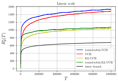
Figure 1: Regret of the various algorithms as a function of time in linear scale.

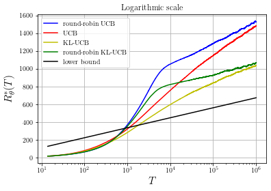
Figure 2: Regret of the various algorithms as a function of time in logarithmic scale.

For our simulations we used the programming language C, to produce highly efficient code, and a personal computer with a 2.6GHz processor and 16GB of memory. We report that the simulation for the Round-Robin KL-UCB adaptive allocation rule was $14.48$ times faster than the simulation for the KL-UCB adaptive allocation rule. This behavior is expected since each calculation of a KL-UCB index induces a significant computation cost as it involves finding the inverse of an increasing function using the bisection method. Additionally, the simulation for the Round-Robin UCB adaptive allocation rule was $3.15$ times faster than the simulation for the KL-UCB adaptive allocation rule, and this is justified from the fact that calculating mathematical functions such as $\log(\cdot)$ and $\sqrt{\cdot}$, is more costly than calculating averages which only involve a division. Our simulation results yield that in practice round-robin schemes are significantly faster than schemes that calculate the indices of all the arms at each round, and the computational gap is increasing with the number of arms $K$, while the behavior of the expected regrets is very similar.

Appendix A Concentration Lemmata for Markov Chains

We first develop a Chernoff bound, which remarkably does not impose any conditions on the Markov chain other than irreducibility, which is though a mandatory requirement for the stationary mean to be well-defined.

Lemma 3 (Chernoff bound for irreducible Markov chains).

Let $\{X_{n}\}_{n\in{{\mathbb{Z}}}_{\geq 0}}$ be an irreducible Markov chain over the finite state space $S$ with transition probability matrix $P$, initial distribution $q$, and stationary distribution $\pi$. Let $f:S\to{{\mathbb{R}}}$ be a nonconstant function on the state space. Denote by $\mu(0)=\sum_{x\in S}f(x)\pi(x)$ the stationary mean when $f$ is applied, and by $\bar{Y}_{n}=\frac{1}{n}\sum_{k=1}^{n}Y_{k}$ the empirical mean, where $Y_{k}=f(X_{k})$. Let $F$ be a closed subset of ${\mathcal{M}}\cap[\mu(0),\infty)$. Then,

$$\operatorname{\mathbb{P}}\left(\bar{Y}_{n}\geq\mu\right)\leq C_{+}e^{-n{D\left({\mu}\;\middle\|\;{\mu(0)}\right)}},~{}\text{for}~{}\mu\in F,$$

where ${D\left({\cdot}\;\middle\|\;{\cdot}\right)}$ stands for the Kullback-Leibler divergence rate in the exponential family of stochastic matrices generated by $P$ and $f$, and $C_{+}=C_{+}(P,f,F)$ is a positive constant depending only on the transition probability matrix $P$, the function $f$ and the closed set $F$.

Proof of Lemma 3..

Using the standard exponential transform followed by Markov’s inequality we obtain that for any $\theta\geq 0$,

$$\operatorname{\mathbb{P}}(\bar{Y}_{n}\geq\mu)\leq\operatorname{\mathbb{P}}(e^{n\theta\bar{Y}_{n}}\geq e^{n\theta\mu})\leq\exp\left\{-n\left(\theta\mu-\frac{1}{n}\log\operatorname{\mathbb{E}}\left[e^{\theta(f(X_{1})+\ldots+f(X_{n}))}\right]\right)\right\}.$$

We can upper bound the expectation from above in the following way,

$$\operatorname{\mathbb{E}}\left[e^{\theta(f(X_{1})+\ldots+f(X_{n}))}\right] =\sum_{x_{0},\ldots,x_{n}\in S}q(x_{0})P(x_{0},x_{1})e^{\theta f(x_{1})}\ldots P(x_{n-1},x_{n})e^{\theta f(x_{n})}$$

$$=\sum_{x_{0},x_{n}\in S}q(x_{0})\tilde{P}_{\theta}^{n}(x_{0},x_{n})$$

$$\leq\frac{1}{\min_{x\in S}v_{\theta}(x)}\sum_{x_{0},x_{n}\in S}q(x_{0})\tilde{P}_{\theta}^{n}(x_{0},x_{n})v_{\theta}(x_{n})$$

$$=\frac{\rho(\theta)^{n}}{\min_{x\in S}v_{\theta}(x)}\sum_{x_{0}\in S}q(x_{0})v_{\theta}(x_{0})$$

$$\leq\max_{x,y\in S}\frac{v_{\theta}(y)}{v_{\theta}(x)}\rho(\theta)^{n},$$

where in the last equality we used the fact that $v_{\theta}$ is a right Perron-Frobenius eigenvector of $\tilde{P}_{\theta}$.

From those two we obtain,

$$\operatorname{\mathbb{P}}(\bar{Y}_{n}\geq\mu)\leq\max_{x,y\in S}\frac{v_{\theta}(y)}{v_{\theta}(x)}\exp\left\{-n(\theta\mu-\Lambda(\theta))\right\},$$

and if we plug in $\theta_{\mu}=\dot{\Lambda}^{-1}(\mu)$, which is a nonnegative real number since $\mu\in F\subseteq{\mathcal{M}}\cap[\mu(0),\infty)$, we obtain,

$$\operatorname{\mathbb{P}}(\bar{Y}_{n}\geq\mu)\leq\max_{x,y\in S}\frac{v_{\theta_{\mu}}(y)}{v_{\theta_{\mu}}(x)}\exp\left\{-n{D\left({\mu}\;\middle\|\;{\mu(0)}\right)}\right\},$$

We assumed that $F$ is closed, and moreover $F$ is bounded since it is a subset of the bounded open interval ${\mathcal{M}}$. Therefore, $F$ is compact, and so $\dot{\Lambda}^{-1}(F)$ is compact as well. Then due to the fact that $\theta\mapsto v_{\theta}(x)/v_{\theta}(y)$ is continuous, from Lemma 2 in Moulos and Anantharam, (2019), we deduce that,

$$\sup_{\theta\in\dot{\Lambda}^{-1}(F)}\max_{x,y\in S}\frac{v_{\theta}(y)}{v_{\theta}(x)}<\infty,$$

which we define to be the finite constant $C_{+}$ of Lemma 3, and which may only depend on $P,f$ and $F$. ∎

Remark 5.

This bound is a variant of Theorem 1 in Moulos and Anantharam, (2019), where the authors derive a Chernoff bound under some structural assumptions on the transition probability matrix $P$ and the function $f$. In our Lemma 3, following their techniques, we derive a Chernoff bound without any assumptions, relying though on the fact that $\mu$ lies in a closed subset of the mean parameter space.

Next, we proceed with the proofs of the lemmata in Section 3.

Proof of Lemma 1..

$$\operatorname{\mathbb{E}}(M_{n+1}^{\theta}\mid{\mathcal{F}}_{n}) =M_{n}^{\theta}\frac{e^{-\Lambda(\theta)}}{v_{\theta}(X_{n})}\operatorname{\mathbb{E}}(v_{\theta}(X_{n+1})e^{\theta f(X_{n+1})}\mid{\mathcal{F}}_{n})$$

$$=M_{n}^{\theta}\frac{e^{-\Lambda(\theta)}}{v_{\theta}(X_{n})}\sum_{x\in S}v_{\theta}(x)e^{\theta f(x)}P(X_{n},y)$$

$$=M_{n}^{\theta}\frac{e^{-\Lambda(\theta)}}{v_{\theta}(X_{n})}\sum_{x\in S}\tilde{P}_{\theta}(X_{n},x)v_{\theta}(x)$$

$$=M_{n}^{\theta},$$

where in the last equality we used the fact that $v_{\theta}$ is a right Perron-Frobenius eigenvector of $\tilde{P}_{\theta}$. ∎

Proof of Lemma 2..

Our proof extends the argument from Lemma 11 in  Cappé et al., (2013), which deals with IID random variables. In order to handle the Markovian dependence we need to use the exponential martingale for Markov chains from Lemma 1, as well as continuity results for the right Perron-Frobenius eigenvector.

Following the proof strategy used to establish the law of the iterated logarithm, we split the range of the union $[n]$ into chunks of exponentially increasing sizes. Denote by $\alpha>1$ the growth factor, to be specified later, and let $n_{m}=\lfloor\alpha^{m}\rfloor$ be the end point of the $m$-th chunk, with $n_{0}=0$. An upper bound on the number of chunks is $M=\lceil\log n/\log\alpha\rceil$, and so we have that

$$\bigcup_{k=1}^{n}\left\{\mu(0)\geq\bar{Y}_{k},~{}k{D\left({\bar{Y}_{k}}\;\middle\|\;{\mu(0)}\right)}\geq\epsilon\right\} \subseteq\bigcup_{m=1}^{M}\bigcup_{k=n_{m-1}+1}^{n_{m}}\left\{\mu(0)\geq\bar{Y}_{k},k{D\left({\bar{Y}_{k}}\;\middle\|\;{\mu(0)}\right)}\geq\epsilon\right\}$$

$$\subseteq\bigcup_{m=1}^{M}\bigcup_{k=n_{m-1}+1}^{n_{m}}\left\{\mu(0)\geq\bar{Y}_{k},{D\left({\bar{Y}_{k}}\;\middle\|\;{\mu(0)}\right)}\geq\frac{\epsilon}{n_{m}}\right\}.$$

Let $\mu_{m}=\inf\{\mu<\mu(0):{D\left({\mu}\;\middle\|\;{\mu(0)}\right)}\leq\epsilon/n_{m}\}$, and $\theta_{m}=\dot{\Lambda}^{-1}(\mu_{m})<\dot{\Lambda}^{-1}(\mu(0))=0$ so that $\theta_{m}\mu_{m}-\Lambda(\theta_{m})={D\left({\mu_{m}}\;\middle\|\;{\mu(0)}\right)}$. Then,

$$\left\{\mu(0)\geq\bar{Y}_{k},~{}{D\left({\bar{Y}_{k}}\;\middle\|\;{\mu(0)}\right)}\geq\frac{\epsilon}{n_{m}}\right\} \subseteq\left\{\bar{Y}_{k}\leq\mu_{m}\right\}$$

$$=\left\{e^{\theta_{m}k\bar{Y}_{k}-k\Lambda(\theta_{m})}\geq e^{k(\theta_{m}\mu_{m}-\Lambda(\theta_{m}))}\right\}$$

$$=\left\{M_{k}^{\theta_{m}}\geq\frac{v_{\theta_{m}}(X_{k})}{v_{\theta_{m}}(X_{0})}e^{k{D\left({\mu_{m}}\;\middle\|\;{\mu(0)}\right)}}\right\}$$

$$\subseteq\left\{M_{k}^{\theta_{m}}\geq\frac{v_{\theta_{m}}(X_{k})}{v_{\theta_{m}}(X_{0})}e^{(n_{m-1}+1){D\left({\mu_{m}}\;\middle\|\;{\mu(0)}\right)}}\right\}.$$

At this point we use the assumption that $P$ is $\left(\operatorname*{arg\,min}_{x\in S}f(x)\right)$-Doeblin in order to invoke Proposition 1 from Moulos and Anantharam, (2019), which in our setting states that there exists a constant $C_{-}=C_{-}(P,f)\geq 1$ such that,

$$\frac{1}{C_{-}}\leq\inf_{\theta\in{{\mathbb{R}}}_{\leq 0},x,y\in S}\frac{v_{\theta}(y)}{v_{\theta}(x)}.$$

This gives us the inclusion,

$$\left\{M_{k}^{\theta_{m}}\geq\frac{v_{\theta_{m}}(X_{k})}{v_{\theta_{m}}(X_{0})}e^{(n_{m-1}+1){D\left({\mu_{m}}\;\middle\|\;{\mu(0)}\right)}}\right\}\subseteq\left\{M_{k}^{\theta_{m}}\geq\frac{e^{(n_{m-1}+1){D\left({\mu_{m}}\;\middle\|\;{\mu(0)}\right)}}}{C_{-}}\right\}.$$

In Lemma 1 we have established that $M_{k}^{\theta_{m}}$ is a positive martingale, which combined with a maximal inequality for martingales due to Ville, (1939) (see Exercise 4.8.2 in Durrett, (2019) for a modern reference), yields that,

$$\operatorname{\mathbb{P}}\left(\bigcup_{k=n_{m-1}+1}^{n_{m}}\left\{M_{k}^{\theta_{m}}\geq\frac{e^{(n_{m-1}+1){D\left({\mu_{m}}\;\middle\|\;{\mu(0)}\right)}}}{C_{-}}\right\}\right) \leq C_{-}e^{-(n_{m-1}+1){D\left({\mu_{m}}\;\middle\|\;{\mu(0)}\right)}}$$

$$\leq C_{-}e^{-\epsilon\frac{n_{m-1}+1}{n_{m}}}\leq C_{-}e^{-\frac{\epsilon}{\alpha}}.$$

To conclude, we pick the growth factor $\alpha=\epsilon/(\epsilon-1)$, and we upper bound the number of chunks by $M\leq\lceil\epsilon\log n\rceil$. ∎

Appendix B Concentration Properties of Upper Confidence Bounds and Sample Means

Lemma 4.

For every arm $a=1,\ldots,K$, and $t\geq 3$, we have that,

$$\operatorname{\mathbb{P}}_{\theta_{a}}\left(\min_{n=1,\ldots,t}U_{n}^{a}(t)\leq\mu(\theta_{a})\right)\leq\frac{4eC_{-}^{a}}{t\log t},$$ (11)

where $C_{-}^{a}$ is the constant prescribed in Lemma 2, when the maximal inequality is applied to the Markov chain with parameter $\theta_{a}$.

Proof.

$$\operatorname{\mathbb{P}}_{\theta_{a}}\left(\min_{n=1,\ldots,t}U_{n}^{a}(t)\leq\mu(\theta_{a})\right) \leq\operatorname{\mathbb{P}}_{\theta_{a}}\left(\bigcup_{n=1}^{t}\{\mu(\theta_{a})>\bar{Y}_{n}^{a}~{}\text{and}~{}n{D\left({\bar{Y}_{n}^{a}}\;\middle\|\;{\mu(\theta_{a})}\right)}\geq g(t)\}\right)$$

$$\leq C_{-}^{a}e\lceil g(t)\log t\rceil e^{-g(t)}\leq 4C_{-}^{a}e(\log t)^{2}e^{-g(t)}=\frac{4eC_{-}^{a}}{t\log t},$$

where for the first inequality we used Equation 8 and the definition of $U_{n}^{a}(t)$, while for the second inequality we used Lemma 2. ∎

Lemma 5.

For every arm $a=1,\ldots,K$, and for $\mu(\lambda)>\mu(\theta_{a})$,

$$\sum_{n=1}^{\infty}\operatorname{\mathbb{P}}_{\theta_{a}}(\mu(\lambda)\leq U_{n}^{a}(T)) \leq\frac{g(T)}{{D\left({\mu(\theta_{a})}\;\middle\|\;{\mu(\lambda)}\right)}}+1+8\sigma_{\theta_{a},\lambda}^{2}\left(\frac{{\dot{D}\left({\mu(\theta_{a})}\;\middle\|\;{\mu(\lambda)}\right)}}{{D\left({\mu(\theta_{a})}\;\middle\|\;{\mu(\lambda)}\right)}}\right)^{2}$$ (12)

$$\qquad+2\sqrt{2\pi\sigma_{\theta_{a},\lambda}^{2}}\sqrt{\frac{{\dot{D}\left({\mu(\theta_{a})}\;\middle\|\;{\mu(\lambda)}\right)}^{2}}{{D\left({\mu(\theta_{a})}\;\middle\|\;{\mu(\lambda)}\right)}^{3}}}\sqrt{g(T)},$$

where $\sigma_{\theta,\lambda}^{2}=\sup_{\theta\in[\theta_{a},\lambda]}\ddot{\Lambda}(\theta)\in(0,\infty)$, and ${\dot{D}\left({\mu(\theta_{a})}\;\middle\|\;{\mu(\lambda)}\right)}=\frac{d{D\left({\mu}\;\middle\|\;{\mu(\lambda)}\right)}}{d\mu}\mid_{\mu=\mu(\theta_{a})}$.

Proof.

The proof is based on the argument given in Appendix A.2 of Cappé et al., (2013), adapted though for the case of Markov chains. If $\mu(\lambda)\leq U_{n}^{a}(T)$, and $\bar{Y}_{n}^{a}\leq\mu(\lambda)$, then ${D\left({\bar{Y}_{n}^{a}}\;\middle\|\;{\mu(\lambda)}\right)}\leq g(T)/n$. Let $\mu_{x}=\inf\{\mu\leq\mu(\lambda):{D\left({\mu}\;\middle\|\;{\mu(\lambda)}\right)}\leq x\}$. This in turn implies that ${D\left({\bar{Y}_{n}^{a}}\;\middle\|\;{\mu(\lambda)}\right)}\leq{D\left({\mu_{g(T)/n}}\;\middle\|\;{\mu(\lambda)}\right)}$, and using the monotonicity of $\mu\mapsto{D\left({\mu}\;\middle\|\;{\mu(\lambda)}\right)}$ for $\mu\leq\mu(\lambda)$, we further have that $\bar{Y}_{n}^{a}\geq\mu_{g(T)/n}$. This argument shows that,

$$\operatorname{\mathbb{P}}_{\theta_{a}}(\mu(\lambda)\leq U_{n}^{a}(T))\leq\operatorname{\mathbb{P}}_{\theta_{a}}(\mu_{g(T)/n}\leq\bar{Y}_{n}^{a}).$$

Therefore,

$$\sum_{n=1}^{\infty}\operatorname{\mathbb{P}}_{\theta_{a}}(\mu(\lambda)\leq U_{n}^{a}(T))\leq\frac{g(T)}{{D\left({\mu(\theta_{a})}\;\middle\|\;{\mu(\lambda)}\right)}}+1+\sum_{n=n_{0}+1}^{\infty}\operatorname{\mathbb{P}}_{\theta_{a}}(\mu_{g(T)/n}\leq\bar{Y}_{n}^{a}),$$

where $n_{0}=\left\lceil\frac{g(T)}{{D\left({\mu(\theta_{a})}\;\middle\|\;{\mu(\lambda)}\right)}}\right\rceil$.

Fix $n\geq n_{0}+1$. Then ${D\left({\mu(\theta_{a})}\;\middle\|\;{\mu(\lambda)}\right)}>g(T)/n$, and therefore $\mu_{g(T)/n}>\mu(\theta_{a})$. Furthermore note that $\mu_{g(T)/n}$ is increasing to $\mu(\lambda)$ as $n$ increases, therefore $\mu_{g(T)/n}$ lives in the closed interval $[\mu(\theta_{a}),\mu(\lambda)]$, and we can apply Lemma 3 for the Markov chain that corresponds to the parameter $\theta_{a}$,

$$\operatorname{\mathbb{P}}_{\theta_{a}}(\bar{Y}_{n}^{a}\geq\mu_{g(T)/n})\leq C_{+}^{a}e^{-n{D\left({\mu_{g(T)/n}}\;\middle\|\;{\mu(\theta_{a})}\right)}}.$$

Thus we are left with the task of controlling the sum,

$$\sum_{n=n_{0}+1}^{\infty}e^{-n{D\left({\mu_{g(T)/n}}\;\middle\|\;{\mu(\theta_{a})}\right)}}.$$

First note that by definition $\mu_{g(T)/n}$ is increasing in $n$, therefore ${D\left({\mu_{g(T)/n}}\;\middle\|\;{\mu(\theta_{a})}\right)}$ is positive and increasing in $n$, hence we can perform the following integral bound,

$$\sum_{n=n_{0}+1}^{\infty}e^{-n{D\left({\mu_{g(T)/n}}\;\middle\|\;{\mu(\theta_{a})}\right)}} \leq\int_{\frac{g(T)}{{D\left({\mu(\theta_{a})}\;\middle\|\;{\mu(\lambda)}\right)}}}^{\infty}e^{-s{D\left({\mu_{g(T)/s}}\;\middle\|\;{\mu(\theta_{a})}\right)}}ds$$

$$=g(T)\int_{0}^{{D\left({\mu(\theta_{a})}\;\middle\|\;{\mu(\lambda)}\right)}}\frac{1}{x^{2}}e^{-\frac{g(T)}{x}{D\left({\mu_{x}}\;\middle\|\;{\mu(\theta_{a})}\right)}}dx.$$ (13)

The function $\mu\mapsto{D\left({\mu}\;\middle\|\;{\mu(\lambda)}\right)}$ is convex thus,

$${D\left({\mu}\;\middle\|\;{\mu(\lambda)}\right)}\geq{D\left({\mu(\theta_{a})}\;\middle\|\;{\mu(\lambda)}\right)}+{\dot{D}\left({\mu(\theta_{a})}\;\middle\|\;{\mu(\lambda)}\right)}(\mu-\mu(\theta_{a})),$$

where ${\dot{D}\left({\mu(\theta_{a})}\;\middle\|\;{\mu(\lambda)}\right)}=\frac{d{D\left({\mu}\;\middle\|\;{\mu(\lambda)}\right)}}{d\mu}\mid_{\mu=\mu(\theta_{a})}$. Plugging in $\mu=\mu_{x}\geq\mu(\theta_{a})$, for $x\in[0,{D\left({\mu(\theta_{a})}\;\middle\|\;{\mu(\lambda)}\right)}]$, we obtain

$${D\left({\mu(\theta_{a})}\;\middle\|\;{\mu(\lambda)}\right)}-x\leq{\dot{D}\left({\mu(\theta_{a})}\;\middle\|\;{\mu(\lambda)}\right)}(\mu(\theta_{a})-\mu_{x}).$$ (14)

From Lemma 8 in Moulos and Anantharam, (2019) we have that,

$${D\left({\mu_{x}}\;\middle\|\;{\mu(\theta_{a})}\right)}\geq\frac{(\mu_{x}-\mu(\theta_{a}))^{2}}{2\sigma_{\theta_{a},\lambda}^{2}},$$ (15)

where $\sigma_{\theta_{a},\lambda}^{2}=\sup_{\theta\in[\theta_{a},\lambda]}\ddot{\Lambda}(\theta)\in(0,\infty)$.

Combining Equation 14 and Equation 15 we deduce that,

$${D\left({\mu_{x}}\;\middle\|\;{\mu(\theta_{a})}\right)}\geq\left(\frac{{D\left({\mu(\theta_{a})}\;\middle\|\;{\mu(\lambda)}\right)}-x}{\sqrt{2}\sigma_{\theta_{a},\lambda}{\dot{D}\left({\mu(\theta_{a})}\;\middle\|\;{\mu(\lambda)}\right)}}\right)^{2}.$$

Now we use this bound and break the integral in Equation 13 in two regions, $I_{1}=[0,{D\left({\mu(\theta_{a})}\;\middle\|\;{\mu(\lambda)}\right)}/2]$ and $I_{2}=[{D\left({\mu(\theta_{a})}\;\middle\|\;{\mu(\lambda)}\right)}/2,{D\left({\mu(\theta_{a})}\;\middle\|\;{\mu(\lambda)}\right)}]$. In the first region we use the fact that $x\leq{D\left({\mu(\theta_{a})}\;\middle\|\;{\mu(\lambda)}\right)}/2$ to deduce that,

$$\int_{I_{1}}\frac{1}{x^{2}}e^{-\frac{g(T)}{x}{D\left({\mu_{x}}\;\middle\|\;{\mu(\theta_{a})}\right)}}dx \leq\int_{I_{1}}\frac{1}{x^{2}}\exp\left\{-\frac{g(T)}{8\sigma_{\theta_{a},\lambda}^{2}x}\left(\frac{{D\left({\mu(\theta_{a})}\;\middle\|\;{\mu(\lambda)}\right)}}{{\dot{D}\left({\mu(\theta_{a})}\;\middle\|\;{\mu(\lambda)}\right)}}\right)^{2}\right\}dx$$

$$\leq\frac{8\sigma_{\theta_{a},\lambda}^{2}}{g(T)}\left(\frac{{\dot{D}\left({\mu(\theta_{a})}\;\middle\|\;{\mu(\lambda)}\right)}}{{D\left({\mu(\theta_{a})}\;\middle\|\;{\mu(\lambda)}\right)}}\right)^{2}.$$

In the second region we use the fact that ${D\left({\mu(\theta_{a})}\;\middle\|\;{\mu(\lambda)}\right)}/2\leq x\leq{D\left({\mu(\theta_{a})}\;\middle\|\;{\mu(\lambda)}\right)}$ to deduce that,

$$\int_{I_{2}}\frac{1}{x^{2}}e^{-\frac{g(T)}{x}{D\left({\mu_{x}}\;\middle\|\;{\mu(\theta_{a})}\right)}}dx \leq\int_{I_{2}}\frac{4\exp\left\{-\frac{(x-{D\left({\mu(\theta_{a})}\;\middle\|\;{\mu(\lambda)}\right)})^{2}}{2\Sigma_{\theta_{a},\lambda}}\right\}}{{D\left({\mu(\theta_{a})}\;\middle\|\;{\mu(\lambda)}\right)}^{2}}dx$$

$$\leq\int_{-\infty}^{{D\left({\mu(\theta_{a})}\;\middle\|\;{\mu(\lambda)}\right)}}\frac{4\exp\left\{-\frac{(x-{D\left({\mu(\theta_{a})}\;\middle\|\;{\mu(\lambda)}\right)})^{2}}{2\Sigma_{\theta_{a},\lambda}}\right\}}{{D\left({\mu(\theta_{a})}\;\middle\|\;{\mu(\lambda)}\right)}^{2}}dx$$

$$=\frac{2\sqrt{2\pi\sigma_{\theta_{a},\lambda}^{2}}}{\sqrt{g(T)}}\sqrt{\frac{{\dot{D}\left({\mu(\theta_{a})}\;\middle\|\;{\mu(\lambda)}\right)}^{2}}{{D\left({\mu(\theta_{a})}\;\middle\|\;{\mu(\lambda)}\right)}^{3}}},$$

where $\Sigma_{\theta_{a},\lambda}=\frac{\sigma_{\theta_{a},\lambda}^{2}{\dot{D}\left({\mu(\theta_{a})}\;\middle\|\;{\mu(\lambda)}\right)}^{2}{D\left({\mu(\theta_{a})}\;\middle\|\;{\mu(\lambda)}\right)}}{g(T)}$. ∎

Lemma 6.

For every arm $a=1,\ldots,K$,

$$\operatorname{\mathbb{P}}_{\theta_{a}}\left(\max_{n=\lceil\delta t\rceil,\ldots,t}|\bar{Y}_{n}^{a}-\mu(\theta_{a})|\geq\epsilon\right)\leq\frac{c\eta^{\delta t}}{1-\eta},~{}\text{for}~{}\delta\in(0,1),~{}\epsilon>0,$$ (16)

where $\eta=\eta({\boldsymbol{\theta}},\epsilon)\in(0,1)$, and $c=c({\boldsymbol{\theta}},\epsilon)$ are constants with respect to $t$.

Proof.

Using the same technique as in the proof of Lemma 3, we have that for any $\theta\geq 0$ and any $\eta\leq 0$,

$$\operatorname{\mathbb{P}}_{\theta_{a}}\left(\max_{n=\lceil\delta t\rceil,\ldots,t}|\bar{Y}_{n}^{a}-\mu(\theta_{a})|\geq\epsilon\right) \leq\sum_{n=\lceil\delta t\rceil}^{\infty}\max_{x,y\in S}\frac{v_{\theta}^{a}(y)}{v_{\theta}^{a}(x)}e^{-n(\theta(\mu(\theta_{a})+\epsilon)-\Lambda_{a}(\theta))}$$

$$\qquad+\sum_{n=\lceil\delta t\rceil}^{\infty}\max_{x,y\in S}\frac{v_{\eta}^{a}(y)}{v_{\eta}^{a}(x)}e^{-n(\eta(\mu(\theta_{a})-\epsilon)-\Lambda_{a}(\eta))},$$

where by $\Lambda_{a}(\theta)$ we denote the log-Perron-Frobenious eigenvalue generated by $P_{\theta_{a}}$, and similarly by $v_{\theta}^{a}$ the corresponding right Perron-Frobenius eigenvector.

By picking $\theta=\theta_{\epsilon}^{a}$ large enough, and $\eta=\eta_{\epsilon}^{a}$ small enough, we can ensure that $\theta(\mu(\theta_{a})+\epsilon)-\Lambda_{a}(\theta)>0$, and $\eta(\mu(\theta_{a})-\epsilon)-\Lambda_{a}(\eta)>0$, and so there are constants $\eta=\eta({\boldsymbol{\theta}},\epsilon)\in(0,1)$ and $c=c({\boldsymbol{\theta}},\epsilon)$, such that for any $a=1,\ldots,K$,

$$\operatorname{\mathbb{P}}_{\theta_{a}}\left(\max_{n=\lceil\delta t\rceil,\ldots,t}|\bar{Y}_{n}^{a}-\mu(\theta_{a})|\geq\epsilon\right)\leq c\sum_{n=\lceil\delta t\rceil}^{\infty}\eta^{n}\leq\frac{c\eta^{\delta t}}{1-\eta}.$$

∎

Appendix C Analysis of Algorithm 1

As a proxy for the regret we will use the following quantity which involves directly the number of times each arm $a\in\{1,\ldots,N\}$ hasn’t been played, and the number of times each arm $b\in\{L+1,\ldots,K\}$ has been played,

$$\tilde{R}_{\boldsymbol{\theta}}^{\boldsymbol{\phi}}(T)=\sum_{a=1}^{N}(\mu(\theta_{a})-\mu(\theta_{M}))\operatorname{\mathbb{E}}_{\boldsymbol{\theta}}^{\boldsymbol{\phi}}[T-N_{a}(T)]\\ +\sum_{b=L+1}^{K}(\mu(\theta_{M})-\mu(\theta_{b}))\operatorname{\mathbb{E}}_{\boldsymbol{\theta}}^{\boldsymbol{\phi}}[N_{b}(T)].$$ (17)

For the IID case $\tilde{R}_{\boldsymbol{\theta}}^{\boldsymbol{\phi}}(T)=R_{\boldsymbol{\theta}}^{\boldsymbol{\phi}}(T)$, and in the more general Markovian case $\tilde{R}_{\boldsymbol{\theta}}^{\boldsymbol{\phi}}(T)$ is just a constant term apart from the expected regret $R_{\boldsymbol{\theta}}^{\boldsymbol{\phi}}(T)$. Note that a feature that makes the case of multiple plays more delicate than the case of single plays, even for IID rewards, is the presence of the first summand in Equation 17. For this we also need to analyze the number of times each of the best $N$ arms hasn’t been played.

Lemma 7.

$$\left|R_{\boldsymbol{\theta}}^{\boldsymbol{\phi}}(T)-\tilde{R}_{\boldsymbol{\theta}}^{\boldsymbol{\phi}}(T)\right|\leq\sum_{a=1}^{K}R_{a}\cdot\sum_{x\in S}|f(x)|,$$

where $R_{a}=\operatorname{\mathbb{E}}_{\theta_{a}}\left[\inf\{n\geq 1:X_{n+1}^{a}=X_{1}^{a}\}\right]<\infty$.

We start the analysis by establishing the relation between the expected regret, Equation 1, and its proxy, Equation 17. For this we will need the following lemma.

Lemma 8 (Lemma 2.1 in Anantharam et al., 1987b ).

Let $\{X_{n}\}_{n\in{{\mathbb{Z}_{\geq 0}}}}$ be a Markov chain on a finite state space $S$, with irreducible transition probability matrix $P$, stationary distribution $\pi$, and initial distribution $q$. Let ${\mathcal{F}}_{n}$ be the $\sigma$-field generated by $X_{0},\ldots,X_{n}$. Let $\tau$ be a stopping time with respect to the filtration $\{{\mathcal{F}}_{n}\}_{n\in{{\mathbb{Z}_{\geq 0}}}}$ such that $\operatorname{\mathbb{E}}[\tau]<\infty$. Define $N(x,n)$ to be the number of visits to state $x$ from time $1$ to time $n$, i.e. $N(x,n)=\sum_{k=1}^{n}I\{X_{k}=x\}$. Then

$$\left|\operatorname{\mathbb{E}}[N(x,\tau)]-\pi(x)\operatorname{\mathbb{E}}[\tau]\right|\leq R,~{}\text{for}~{}x\in S,$$

where $R=\operatorname{\mathbb{E}}[\inf\{n\geq 1:X_{n+1}=X_{1}\}]<\infty$.

Proof of Lemma 7..

First note that,

$$S_{T}=\sum_{a=1}^{K}\sum_{x\in S}f(x)N_{a}(x,N_{a}(T)).$$

For each $a\in[K]$, using first the triangle inequality, and then Lemma 8 for the stopping time $N_{a}(T)$, we obtain,

$$\left|\sum_{x\in S}f(x)(\operatorname{\mathbb{E}}_{\boldsymbol{\theta}}^{\boldsymbol{\phi}}[N_{a}(x,N_{a}(T))]-\pi_{\theta_{a}}(x)\operatorname{\mathbb{E}}_{\boldsymbol{\theta}}^{\boldsymbol{\phi}}[N_{a}(T)])\right|$$

$$\qquad\leq\sum_{x\in S}|f(x)|\left|\operatorname{\mathbb{E}}_{\boldsymbol{\theta}}^{\boldsymbol{\phi}}[N_{a}(x,N_{a}(T))]-\pi_{\theta_{a}}(x)\operatorname{\mathbb{E}}_{\boldsymbol{\theta}}^{\boldsymbol{\phi}}[N_{a}(T)]\right|$$

$$\qquad\leq R_{a}\cdot\sum_{x\in S}|f(x)|.$$

Hence summing over $a\in[K]$, and using the triangle inequality, we see that,

$$\left|S_{T}-\sum_{a=1}^{K}\mu(\theta_{a})\operatorname{\mathbb{E}}_{\boldsymbol{\theta}}^{\boldsymbol{\phi}}[N_{a}(T)]\right|\leq\sum_{a=1}^{K}R_{a}\cdot\sum_{x\in S}|f(x)|.$$

To conclude the proof note that,

$$T\sum_{a=1}^{M}\mu(\theta_{a})-\sum_{a=1}^{K}\mu(\theta_{a})\operatorname{\mathbb{E}}_{\boldsymbol{\theta}}^{\boldsymbol{\phi}}[N_{a}(T)]$$

$$\qquad=\sum_{a=1}^{N}\mu(\theta_{a})\operatorname{\mathbb{E}}_{\boldsymbol{\theta}}^{\boldsymbol{\phi}}[T-N_{a}(T)]+\mu(\theta_{M})(M-N)-\mu(\theta_{M})\sum_{a=N+1}^{K}\operatorname{\mathbb{E}}_{\boldsymbol{\theta}}^{\boldsymbol{\phi}}[N_{a}(T)]$$

$$\qquad\qquad+\sum_{b=L+1}^{K}(\mu(\theta_{M})-\mu(\theta_{b}))\operatorname{\mathbb{E}}_{\boldsymbol{\theta}}^{\boldsymbol{\phi}}[N_{b}(T)]$$

$$\qquad=\sum_{a=1}^{N}(\mu(\theta_{a})-\mu(\theta_{M}))\operatorname{\mathbb{E}}_{\boldsymbol{\theta}}^{\boldsymbol{\phi}}[T-N_{a}(T)]+\sum_{b=L+1}^{K}(\mu(\theta_{M})-\mu(\theta_{b}))\operatorname{\mathbb{E}}_{\boldsymbol{\theta}}^{\boldsymbol{\phi}}[N_{b}(T)],$$

where in the last equality we used the fact that $\sum_{a=1}^{N}\operatorname{\mathbb{E}}_{\boldsymbol{\theta}}^{\boldsymbol{\phi}}[N_{a}(T)]+\sum_{a=N+1}^{K}\operatorname{\mathbb{E}}_{\boldsymbol{\theta}}^{\boldsymbol{\phi}}[N_{a}(T)]=TM$. ∎

Next we show that Algorithm 1 is well-defined.

Proof of Proposition 1..

Recall that $\sum_{a\in[K]}N_{a}(t)=tM$, and so there exists an arm $a_{1}$ such that $N_{a_{1}}(t)\geq tM/K$. Then $\sum_{a\in[K]-\{a_{1}\}}N_{a}(t)\geq t(M-1)$, and so there exists an arm $a_{2}\neq a_{1}$ such that $N_{a_{2}}(t)\geq t(M-1)/(K-1)$. Inductively we can see that there exist $M$ distinct arms $a_{1},\ldots,a_{M}$ such that $N_{a_{i}}(t)\geq t(M-i+1)/(K-i+1)\geq t/K>\delta t$, for $i=1,\ldots,M$. ∎

C.1 Sketch for the rest of the analysis

Due to Lemma 7, it suffices to upper bound the proxy for the expected regret given in Equation 17. Therefore, we can break the analysis in two parts: upper bounding $\operatorname{\mathbb{E}}_{\boldsymbol{\theta}}^{\boldsymbol{\phi}}[T-N_{a}(T)]$, for $a=1,\ldots,N$, and upper bounding $\operatorname{\mathbb{E}}_{\boldsymbol{\theta}}^{\boldsymbol{\phi}}[N_{b}(T)]$, for $b=L+1,\ldots,K$.

For the first part, we show in Appendix C that the expected number of times that an arm $a\in\{1,\ldots,N\}$ hasn’t been played, is of the order of $O(\log\log T)$.

Lemma 9.

For every arm $a=1,\ldots,N$,

$$\operatorname{\mathbb{E}}_{\boldsymbol{\theta}}^{\boldsymbol{\phi}}[T-N_{a}(T)]\leq\frac{4e\gamma^{2}NC\left\lceil\frac{2\log\gamma}{\log\frac{1}{\delta}}\right\rceil}{\log\gamma}\log\log T+\gamma^{r_{0}}+\frac{c\gamma^{2}\eta^{\delta}K}{(1-\eta)(1-\eta^{\delta})^{3}},$$

where $\gamma,r_{0},\eta,c$ and $C$ are constants with respect to $T$.

For the second part, if $b\in\{L+1,\ldots,K\}$, and $b\in\phi_{t+1}$, then there are three possibilities:

1. $L_{t}\subseteq[L]$, and $|\bar{Y}_{a}(t)-\mu(\theta_{a})|\geq\epsilon$ for some $a\in L_{t}$,

2. $L_{t}\subseteq[L]$, and $|\bar{Y}_{a}(t)-\mu(\theta_{a})|<\epsilon$ for all $a\in L_{t}$, and $b\in\phi_{t+1}$,

3. $L_{t}\cap\{L+1,\ldots,K\}\neq\emptyset$.

This means that,

$$\operatorname{\mathbb{E}}_{\boldsymbol{\theta}}^{\boldsymbol{\phi}}[N_{b}(T)] \leq M+\sum_{t=K}^{T-1}\operatorname{\mathbb{P}}_{\boldsymbol{\theta}}^{\boldsymbol{\phi}}\left(L_{t}\subseteq[L],~{}\text{and}~{}|\bar{Y}_{a}(t)-\mu(\theta_{a})|\geq\epsilon~{}\text{for some}~{}a\in L_{t}\right)$$

$$\quad+\sum_{t=K}^{T-1}\operatorname{\mathbb{P}}_{\boldsymbol{\theta}}^{\boldsymbol{\phi}}\left(L_{t}\subseteq[L],~{}\text{and}~{}|\bar{Y}_{a}(t)-\mu(\theta_{a})|<\epsilon~{}\text{for all}~{}a\in L_{t},~{}\text{and}~{}b\in\phi_{t+1}\right)$$

$$\quad+\sum_{t=K}^{T-1}\operatorname{\mathbb{P}}_{\boldsymbol{\theta}}^{\boldsymbol{\phi}}(L_{t}\cap\{L+1,\ldots,K\}\neq\emptyset),$$

and we handle each of those three terms separately.

We show that the first term is upper bounded by $O(1)$.

Lemma 10.

$$\sum_{t=K}^{T-1}\operatorname{\mathbb{P}}_{\boldsymbol{\theta}}^{\boldsymbol{\phi}}\left(L_{t}\subseteq[L],~{}\text{and}~{}|\bar{Y}_{a}(t)-\mu(\theta_{a})|\geq\epsilon~{}\text{for some}~{}a\in L_{t}\right)\leq\frac{cL\eta^{\delta K}}{(1-\eta)(1-\eta^{\delta})},$$

where $c$ and $\eta$ are constant with respect to $T$.

The second term is of the order of $O(\log T)$, and it is the term that causes the overall logarithmic regret.

Lemma 11.

$$\sum_{t=K}^{T-1}\operatorname{\mathbb{P}}_{\boldsymbol{\theta}}^{\boldsymbol{\phi}}\left(L_{t}\subseteq[L],~{}\text{and}~{}|\bar{Y}_{a}(t)-\mu(\theta_{a})|<\epsilon~{}\text{for all}~{}a\in L_{t},~{}\text{and}~{}b\in\phi_{t+1}\right)$$

$$\qquad\leq\frac{\log T+3\log\log T}{{D\left({\mu(\theta_{b})}\;\middle\|\;{\mu(\theta_{M})-\epsilon}\right)}}+1+8\sigma_{\mu(\theta_{a}),\mu(\theta_{M})-\epsilon}^{2}\left(\frac{{\dot{D}\left({\mu(\theta_{b})}\;\middle\|\;{\mu(\theta_{M})-\epsilon}\right)}}{{D\left({\mu(\theta_{b})}\;\middle\|\;{\mu(\theta_{M})-\epsilon}\right)}}\right)^{2}$$

$$\qquad\qquad+2\sqrt{2\pi\sigma_{\mu(\theta_{a}),\mu(\theta_{M})-\epsilon}^{2}}\sqrt{\frac{{\dot{D}\left({\mu(\theta_{b})}\;\middle\|\;{\mu(\theta_{M})-\epsilon}\right)}^{2}}{{D\left({\mu(\theta_{b})}\;\middle\|\;{\mu(\theta_{M})-\epsilon}\right)}^{3}}}\left(\sqrt{\log T}+\sqrt{3\log\log T}\right),$$

where $\sigma_{\mu(\theta_{a}),\mu(\theta_{M})-\epsilon}^{2}$, and ${\dot{D}\left({\mu(\theta_{b})}\;\middle\|\;{\mu(\theta_{M})-\epsilon}\right)}=\frac{d{D\left({\mu}\;\middle\|\;{\mu(\theta_{M})-\epsilon}\right)}}{d\mu}\mid_{\mu=\mu(\theta_{b})}$, are constants with respect to $T$.

Finally, we show that the third term is upper bounded by $O(\log\log T)$.

Lemma 12.

$$\sum_{t=K}^{T-1}\operatorname{\mathbb{P}}_{\boldsymbol{\theta}}^{\boldsymbol{\phi}}(L_{t}\cap\{L+1,\ldots,K\}\neq\emptyset)\leq\frac{4e\gamma^{2}LC\left\lceil\frac{2\log\gamma}{\log\frac{1}{\delta}}\right\rceil}{\log\gamma}\log\log T+\gamma^{r_{0}}+\frac{c\gamma^{2}\eta^{\delta}K}{(1-\eta)(1-\eta^{\delta})^{3}},$$

where $\gamma,r_{0},\eta,c$ and $C$ are constants with respect to $T$.

This concludes the proof of Theorem 1, modulo the four bounds of this subsection which are established in the next subsection.

C.2 Proofs for the four bounds

For the rest of the analysis we define the following events which describe good behavior of the sample means and the upper confidence bounds. For $\gamma,r\in\mathbb{Z}_{>1}$ let,

$$A_{r} =\bigcap_{a\in[K]}\bigcap_{\gamma^{r-1}\leq t\leq\gamma^{r+1}}\left\{\max_{n=\lceil\delta t\rceil,\ldots,t}|\bar{Y}_{n}^{a}-\mu(\theta_{a})|<\epsilon\right\},$$

$$B_{r} =\bigcap_{a\in[N]}\bigcap_{\gamma^{r-1}\leq t\leq\gamma^{r+1}}\left\{\min_{n=1,\ldots,\lceil\delta t\rceil-1}U_{n}^{a}(t)>\mu(\theta_{N})\right\},$$

$$C_{r} =\bigcap_{a\in[L]}\bigcap_{\gamma^{r-1}\leq t\leq\gamma^{r+1}}\left\{\min_{n=1,\ldots,\lceil\delta t\rceil-1}U_{n}^{a}(t)>\mu(\theta_{a})\right\}.$$

Indeed, the following bounds, which rely on the concentration results of Section 3, suggest that those events will happen with some good probability.

Lemma 13.

$$\operatorname{\mathbb{P}}_{\boldsymbol{\theta}}(A_{r}^{c})\leq\frac{cK\eta^{\delta\gamma^{r-1}}}{(1-\eta)(1-\eta^{\delta})},\quad\operatorname{\mathbb{P}}_{\boldsymbol{\theta}}(B_{r}^{c})\leq\frac{4eNC\left\lceil\frac{2\log\gamma}{\log\frac{1}{\delta}}\right\rceil}{(r-1)\gamma^{r-1}\log\gamma},\quad\operatorname{\mathbb{P}}_{\boldsymbol{\theta}}(C_{r}^{c})\leq\frac{4eLC\left\lceil\frac{2\log\gamma}{\log\frac{1}{\delta}}\right\rceil}{(r-1)\gamma^{r-1}\log\gamma},$$

where $\eta\in(0,1),~{}c$ and $C$ are constants with respect to $r$.

Proof.

The first bound follows directly from Equation 16 and a union bound.

For the second bound, let $p=\left\lceil\frac{2\log\gamma}{\log\frac{1}{\delta}}\right\rceil$, so that $\left\lfloor\frac{\gamma^{r-1}}{\delta^{p}}\right\rfloor\geq\gamma^{r+1}$. For $i=0,\ldots,p$ let $t_{i}=\left\lfloor\frac{\gamma^{r-1}}{\delta^{i}}\right\rfloor$, and define,

$$D_{i}=\bigcap_{a\in[N]}\left\{\min_{n=1,\ldots,t_{i}}U_{n}^{a}(t)>\mu(\theta_{a})\right\}.$$

From Equation 11 we see that,

$$\operatorname{\mathbb{P}}_{{\boldsymbol{\theta}}}(D_{i}^{c})\leq\frac{4eN\max_{a\in[N]}C_{-}^{a}}{t_{i}\log t_{i}}\leq\frac{4eN\max_{a\in[N]}C_{-}^{a}}{(r-1)\gamma^{r-1}\log\gamma},$$

where $C_{-}^{a}$ is the constant from Lemma 2.

Fix $a\in[N]$, and $\gamma^{r-1}\leq t\leq\gamma^{r+1}$. There exists $i\in\{0,\ldots,p-1\}$ such that $t_{i}\leq t\leq t_{i+1}$, and so $t_{i}>\delta t_{i}-1\geq\delta t-1$, which gives that $t_{i}\geq\lceil\delta t\rceil-1$. On $D_{i}$, due to Equation 9, we have that,

$$\min_{n=1,\ldots,\lceil\delta t\rceil-1}U_{n}^{a}(t)\geq\min_{n=1,\ldots,\lceil\delta t\rceil-1}U_{n}^{a}(t_{i})\geq\min_{n=1,\ldots,t_{i}}U_{n}^{a}(t_{i})>\mu(\theta_{a})\geq\mu(\theta_{N}).$$

Therefore,

$$\operatorname{\mathbb{P}}_{\boldsymbol{\theta}}(B_{r}^{c})\leq\sum_{i=0}^{p-1}\operatorname{\mathbb{P}}_{\boldsymbol{\theta}}(D_{i}^{c})\leq\frac{4eNp\max_{a\in[N]}C_{-}^{a}}{(r-1)\gamma^{r-1}\log\gamma}.$$

The third bound is established along the same lines. ∎

In order to establish Lemma 9 we need the following lemma which states that, on $A_{r}\cap B_{r}$, an event of sufficiently large probability according to Lemma 13, all the best $N$ arms are played.

Lemma 14 (Lemma 5.3 in Anantharam et al., 1987a ).

Fix $\gamma\geq\lceil(1-K\delta)^{-1}\rceil+2$, and let $r_{0}=\lceil\log_{\gamma}\frac{2K}{1-K\delta-\gamma^{-1}}\rceil+2$. For any $r\geq r_{0}$, on $A_{r}\cap B_{r}$ we have that $[N]\subset\phi_{t+1}$ for all $\gamma^{r}\leq t\leq\gamma^{r+1}$.

Proof of Lemma 9..

$$\operatorname{\mathbb{E}}_{\boldsymbol{\theta}}^{\boldsymbol{\phi}}[T-N_{a}(T)] \leq\gamma^{r_{0}}+\sum_{r=r_{0}}^{\lceil\log_{\gamma}(T-1)\rceil-1}\sum_{\gamma^{r}\leq t\leq\gamma^{r+1}}\operatorname{\mathbb{P}}_{\boldsymbol{\theta}}^{\boldsymbol{\phi}}(a\not\in\phi_{t+1})$$

$$\leq\gamma^{r_{0}}+\sum_{r=r_{0}}^{\lceil\log_{\gamma}(T-1)\rceil-1}\sum_{\gamma^{r}\leq t\leq\gamma^{r+1}}(\operatorname{\mathbb{P}}_{\boldsymbol{\theta}}(A_{r}^{c})+\operatorname{\mathbb{P}}_{\boldsymbol{\theta}}(B_{r}^{c}))$$

$$\leq\gamma^{r_{0}}+\sum_{r=r_{0}}^{\lceil\log_{\gamma}(T-1)\rceil-1}\left(\frac{cK\gamma^{r+1}\eta^{\delta\gamma^{r-1}}}{(1-\eta)(1-\eta^{\delta})}+\frac{4e\gamma^{2}NC\left\lceil\frac{2\log\gamma}{\log\frac{1}{\delta}}\right\rceil}{(r-1)\log\gamma}\right),$$

where the second inequality follows from Lemma 14, and the third from Lemma 13. Now we use a simple logarithmic upper bound on the harmonic number to obtain,

$$\sum_{r=r_{0}}^{\lceil\log_{\gamma}(T-1)\rceil-1}\frac{1}{r-1}\leq\sum_{r=3}^{\lceil\log_{\gamma}(T-1)\rceil-1}\frac{1}{r-1}\leq\log\log_{\gamma}T\leq\log\log T.$$

Finally, we can upper bound the other summand by a constant, with respect to $T$, in the following way,

$$\sum_{r=r_{0}}^{\lceil\log_{\gamma}(T-1)\rceil-1}\gamma^{r-1}\eta^{\delta\gamma^{r-1}}\leq\sum_{k=1}^{\infty}k\eta^{\delta k}=\frac{\eta^{\delta}}{(1-\eta^{\delta})^{2}}.$$

∎

Proof of Lemma 10..

Using Equation 16 it is straightforward to see that

$$\operatorname{\mathbb{P}}_{\boldsymbol{\theta}}^{\boldsymbol{\phi}}\left(L_{t}\subseteq[L],~{}\text{and}~{}|\bar{Y}_{a}(t)-\mu(\theta_{a})|\geq\epsilon~{}\text{for some}~{}a\in L_{t}\right)\leq\frac{cL\eta^{\delta t}}{1-\eta},$$

and the conclusion follows by summing the geometric series. ∎

Proof of Lemma 11..

Assume that $L_{t}\subseteq[L]$, and $|\bar{Y}_{a}(t)-\mu(\theta_{a})|<\epsilon$ for all $a\in L_{t}$, and $b\in\phi_{t+1}$. Then it must be the case that $b\equiv t+1\pmod{K},~{}b\not\in L_{t}$, and $U_{b}(t)>\min_{a\in L_{t}}\bar{Y}_{a}(t)>\min_{a\in L_{t}}\mu(\theta_{a})-\epsilon\geq\mu(\theta_{M})-\epsilon$. This shows that,

$$\operatorname{\mathbb{P}}_{\boldsymbol{\theta}}^{\boldsymbol{\phi}}\left(L_{t}\subseteq[L],~{}\text{and}~{}|\bar{Y}_{a}(t)-\mu(\theta_{a})|<\epsilon~{}\text{for all}~{}a\in L_{t},~{}\text{and}~{}b\in\phi_{t+1}\right)$$

$$\qquad\leq\operatorname{\mathbb{P}}_{\boldsymbol{\theta}}^{\boldsymbol{\phi}}(b\in\phi_{t+1},~{}\text{and}~{}U_{b}(t)>\mu(\theta_{M})-\epsilon).$$

Furthermore,

$$\sum_{t=K}^{T-1}\operatorname{\mathbb{P}}_{\boldsymbol{\theta}}^{\boldsymbol{\phi}}(b\in\phi_{t+1},~{}\text{and}~{}U_{b}(t)>\mu(\theta_{M})-\epsilon)$$

$$\qquad=\sum_{t=K}^{T-1}\sum_{n=M+1}^{M+T-K}\operatorname{\mathbb{P}}_{\boldsymbol{\theta}}^{\boldsymbol{\phi}}(\tau_{n}^{b}=t+1,~{}\text{and}~{}U_{n}^{b}(t)>\mu(\theta_{M})-\epsilon)$$

$$\qquad\leq\sum_{t=K}^{T-1}\sum_{n=M+1}^{M+T-K}\operatorname{\mathbb{P}}_{\boldsymbol{\theta}}^{\boldsymbol{\phi}}(\tau_{n}^{b}=t+1,~{}\text{and}~{}U_{n}^{b}(T)>\mu(\theta_{M})-\epsilon)$$

$$\qquad=\sum_{n=M+1}^{M+T-K}\sum_{t=K}^{T-1}\operatorname{\mathbb{P}}_{\boldsymbol{\theta}}^{\boldsymbol{\phi}}(\tau_{n}^{b}=t+1,~{}\text{and}~{}U_{n}^{b}(T)>\mu(\theta_{M})-\epsilon)$$

$$\qquad\leq\sum_{n=M+1}^{M+T-K}\operatorname{\mathbb{P}}_{\theta_{b}}(U_{n}^{b}(T)>\mu(\theta_{M})-\epsilon),$$

where in the first inequality we used Equation 9. Now the conclusion follows from Equation 12. ∎

In order to establish Lemma 12 we need the following lemma which states that, on $A_{r}\cap C_{r}$, an event of sufficiently large probability according to Lemma 13, only arms from $\{1,\ldots,L\}$ have been played at least $\lceil\delta t\rceil$ times and have a large sample mean.

Lemma 15 (Lemma 5.3 B in Anantharam et al., 1987a ).

Fix $\gamma\geq\lceil(1-K\delta)^{-1}\rceil+2$, and let $r_{0}=\lceil\log_{\gamma}\frac{2K}{1-K\delta-\gamma^{-1}}\rceil+2$. For any $r\geq r_{0}$, on $A_{r}\cap C_{r}$ we have that $L_{t}\subseteq[L]$ for all $\gamma^{r}\leq t\leq\gamma^{r+1}$.

Proof of Lemma 12..

From Lemma 15 we see that,

$$\sum_{t=K}^{T-1}\operatorname{\mathbb{P}}_{\boldsymbol{\theta}}^{\boldsymbol{\phi}}(L_{t}\cap\{L+1,\ldots,K\}\neq\emptyset)\leq\gamma^{r_{0}}+\sum_{r=r_{0}}^{\lceil\log_{\gamma}(T-1)\rceil-1}\sum_{\gamma^{r}\leq t\leq\gamma^{r+1}}(\operatorname{\mathbb{P}}_{\boldsymbol{\theta}}(A_{r}^{c})+\operatorname{\mathbb{P}}_{\boldsymbol{\theta}}(C_{r}^{c})).$$

The rest of the calculations are similar with the proof of Lemma 9. ∎

Proof of Corollary 1..

In the finite-time regret bound of Theorem 1 we divide by $\log T$, let $T$ go to $\infty$, and then let $\epsilon$ go to $0$ in order to get,

$$\limsup_{T\to\infty}\frac{R_{\boldsymbol{\theta}}^{\boldsymbol{\phi}}(T)}{\log T}\leq\sum_{b=L+1}^{K}\frac{\mu(\theta_{M})-\mu(\theta_{b})}{{D\left({\mu(\theta_{b})}\;\middle\|\;{\mu(\theta_{M})}\right)}}.$$

The conclusion now follows by using the asymptotic lower bound from Equation 3. ∎

Proof of Theorem 2..

The proof of Theorem 2 follows along the lines the proof of Theorem 1, by replacing instances of entries of the right Perron-Frobenius eigenvector $v_{\theta}(x)$ with one, and is thus omitted. ∎

Appendix D General Asymptotic Lower Bound

Recall from Subsection 2.1 the general one-parameter family of Markov chains $\{\operatorname{\mathbb{P}}_{\theta}:\theta\in\Theta\}$, where each Markovian probability law $\operatorname{\mathbb{P}}_{\theta}$ is characterized by an initial distribution $q_{\theta}$ and a transition probability matrix $P_{\theta}$. For this family we assume that,

$$P_{\theta}~{}\text{is irreducible for all}~{}\theta\in\Theta.$$ (18)

$$P_{\theta}(x,y)>0\;\Rightarrow\;P_{\lambda}(x,y)>0,~{}\text{for all}~{}\theta,\lambda\in\Theta,~{}x,y\in S.$$ (19)

$$q_{\theta}(x)>0\;\Rightarrow\;q_{\lambda}(x),~{}\text{for all}~{}\theta,\lambda\in\Theta,~{}x\in S.$$ (20)

In general it is not necessary that the parameter space $\Theta$ is the whole real line, but it is assumed to satisfy the following denseness condition. For all $\lambda\in\Theta$ and all $\delta>0$, there exists $\lambda^{\prime}\in\Theta$ such that,

$$\mu(\lambda)<\mu(\lambda^{\prime})<\mu(\lambda)+\delta.$$ (21)

Furthermore, the Kullback-Leibler divergence rate is assumed to satisfy the following continuity property. For all $\epsilon>0$, and for all $\theta,\lambda\in\Theta$ such that $\mu(\lambda)>\mu(\theta)$, there exists $\delta>0$ such that,

$$\mu(\lambda)<\mu(\lambda^{\prime})<\mu(\lambda)+\delta\;\Rightarrow\;|{D\left({\theta}\;\middle\|\;{\lambda}\right)}-{D\left({\theta}\;\middle\|\;{\lambda^{\prime}}\right)}|<\epsilon.$$ (22)

An adaptive allocation rule ${\boldsymbol{\phi}}$ is called uniformly good if,

$$R_{\boldsymbol{\theta}}^{\boldsymbol{\phi}}(T)=o(T^{\alpha}),~{}\text{for all}~{}{\boldsymbol{\theta}}\in\Theta^{K},~{}\text{and all}~{}\alpha>0.$$

Under those conditions Anantharam et al., 1987b establish the following asymptotic lower bound.

Theorem 3 (Theorem 3.1 from Anantharam et al., 1987b ).

Assume that the one-parameter family of Markov chains on the finite state space $S$, together with the reward function $f:S\to{{\mathbb{R}}}$, satisfy conditions (18), (19), (20), (21), and (22). Let ${\boldsymbol{\phi}}$ be a uniformly good allocation rule. Fix a parameter configuration ${\boldsymbol{\theta}}\in\Theta^{K}$, and without loss of generality assume that,

$$\mu(\theta_{1})\geq\ldots\geq\mu(\theta_{N})>\mu(\theta_{N+1})\ldots=\mu(\theta_{M})=\ldots=\mu(\theta_{L})>\mu(\theta_{L+1})\geq\ldots\geq\mu(\theta_{K}).$$

Then for every $b=L+1,\ldots,K$,

$$\frac{1}{{D\left({\theta_{b}}\;\middle\|\;{\theta_{M}}\right)}}\leq\liminf_{T\to\infty}\frac{\operatorname{\mathbb{E}}_{\boldsymbol{\theta}}^{\boldsymbol{\phi}}\left[N_{b}(T)\right]}{\log T}.$$

Consequently,

$$\sum_{b=L+1}^{K}\frac{\mu(\theta_{M})-\mu(\theta_{b})}{{D\left({\theta_{b}}\;\middle\|\;{\theta_{M}}\right)}}\leq\liminf_{T\to\infty}\frac{R_{\boldsymbol{\theta}}^{\boldsymbol{\phi}}(T)}{\log T}.$$

Lower bounds on the expected regret of multi-armed bandit problems are established using a change of measure argument, which relies on the adaptive allocation rule being uniformly good. Lai and Robbins, (1985) gave the prototypical change of measure argument, for the case of i.i.d. rewards, and Anantharam et al., 1987b extended this technique for the case of Markovian rewards. Here we give an alternative simplified proof using the data processing inequality, an idea introduced in Kaufmann et al., (2016); Combes and Proutiere, (2014) for the i.i.d. case.

We first set up some notation. Denote by ${\mathcal{F}}_{T}$ the $\sigma$-field generated by the random variables $\phi_{1},\ldots,\phi_{T},\{X_{n}^{1}\}_{n=0}^{N_{1}(T)},\ldots,\{X_{n}^{K}\}_{n=0}^{N_{K}(T)}$, and let $\operatorname{\mathbb{P}}_{\boldsymbol{\theta}}^{\boldsymbol{\phi}}\mid_{{\mathcal{F}}_{T}}$ be the restriction of the probability distribution $\operatorname{\mathbb{P}}_{\boldsymbol{\theta}}^{\boldsymbol{\phi}}$ on ${\mathcal{F}}_{T}$. For two probability distributions $\operatorname{\mathbb{P}}$ and $\operatorname{\mathbb{Q}}$ over the same measurable space we define the Kullback-Leibler divergence between $\operatorname{\mathbb{P}}$ and $\operatorname{\mathbb{Q}}$ as

$${D\left({\operatorname{\mathbb{P}}}\;\middle\|\;{\operatorname{\mathbb{Q}}}\right)}=\begin{cases}\operatorname{\mathbb{E}}_{\operatorname{\mathbb{P}}}\left[\log\frac{d\operatorname{\mathbb{P}}}{d\operatorname{\mathbb{Q}}}\right],&\text{if}~{}\operatorname{\mathbb{P}}\ll\operatorname{\mathbb{Q}},\\ \infty,&\text{otherwise},\end{cases}$$

where $\frac{d\operatorname{\mathbb{P}}}{d\operatorname{\mathbb{Q}}}$ denotes the Radon-Nikodym derivative, when $\operatorname{\mathbb{P}}$ is absolutely continuous with respect to $\operatorname{\mathbb{Q}}$. Note that we have used the same notation as for the Kullback-Leibler divergence rate between two Markov chains, but it should be clear from the arguments whether we refer to the divergence or the divergence rate. For $p,q\in[0,1]$, the binary Kullback-Leibler divergence is denoted by

$${D_{2}\left({p}\;\middle\|\;{q}\right)}=p\log\frac{p}{q}+(1-p)\log\frac{1-p}{1-q}.$$

The following lemma, from Moulos, (2019), will be crucial in establishing the lower bound.

Lemma 16 (Lemma 1 in Moulos, (2019)).

Let ${\boldsymbol{\theta}},{\boldsymbol{\lambda}}\in\Theta^{K}$ be two parameter configurations. Let $\tau$ be a stopping time with respect to $({\mathcal{F}}_{t})_{t\in{{\mathbb{Z}_{>0}}}}$, with $\operatorname{\mathbb{E}}_{\boldsymbol{\theta}}^{\boldsymbol{\phi}}[\tau],~{}\operatorname{\mathbb{E}}_{\boldsymbol{\lambda}}^{\boldsymbol{\phi}}[\tau]<\infty$. Then

$${D\left({\operatorname{\mathbb{P}}_{\boldsymbol{\theta}}^{\boldsymbol{\phi}}\mid_{{\mathcal{F}}_{\tau}}}\;\middle\|\;{\operatorname{\mathbb{P}}_{\boldsymbol{\lambda}}^{\boldsymbol{\phi}}\mid_{{\mathcal{F}}_{\tau}}}\right)}\leq\sum_{a=1}^{K}{D\left({q_{\theta_{a}}}\;\middle\|\;{q_{\lambda_{a}}}\right)}+\sum_{a=1}^{K}\left(\operatorname{\mathbb{E}}_{\boldsymbol{\theta}}^{\boldsymbol{\phi}}[N_{a}(\tau)]+R_{\theta_{a}}\right){D\left({\theta_{a}}\;\middle\|\;{\lambda_{a}}\right)},$$

where $R_{\theta_{a}}=\operatorname{\mathbb{E}}_{\theta_{a}}\>\left[\inf\{n\geq 1:X_{n+1}^{a}=X_{1}^{a}\}\right]<\infty$, the first summand is finite due to (20), and the second summand is finite due to (19).

Proof of Theorem 3..

Fix $b\in\{L+1,\ldots,K\}$, and $\epsilon>0$. Due to Equation 21 and Equation 22, there exists $\lambda\in\Theta$ such that

$$\mu(\theta_{M})<\mu(\lambda),~{}\text{and}~{}|{D\left({\theta_{b}}\;\middle\|\;{\theta_{M}}\right)}-{D\left({\theta_{b}}\;\middle\|\;{\lambda}\right)}|<\epsilon.$$

We consider the parameter configuration ${\boldsymbol{\lambda}}=(\lambda_{1},\ldots,\lambda_{K})$ given by,

$$\lambda_{a}=\begin{cases}\theta_{a},&\text{if}~{}a\neq b,\\ \lambda,&\text{if}~{}a=b.\end{cases}$$

Using Lemma 16 we obtain,

$${D\left({\operatorname{\mathbb{P}}_{\boldsymbol{\theta}}^{\boldsymbol{\phi}}\mid_{{\mathcal{F}}_{T}}}\;\middle\|\;{\operatorname{\mathbb{P}}_{\boldsymbol{\lambda}}^{\boldsymbol{\phi}}\mid_{{\mathcal{F}}_{T}}}\right)}\leq{D\left({q_{\theta_{b}}}\;\middle\|\;{q_{\lambda}}\right)}+R_{\theta_{b}}{D\left({\theta_{b}}\;\middle\|\;{\lambda}\right)}+\operatorname{\mathbb{E}}_{\boldsymbol{\theta}}^{\boldsymbol{\phi}}\left[N_{b}(T)\right]{D\left({\theta_{b}}\;\middle\|\;{\lambda}\right)}.$$

From the data processing inequality, see the book of Cover and Thomas, (2006), we have that for any event ${\mathcal{E}}\in{\mathcal{F}}_{T}$,

$${D_{2}\left({\operatorname{\mathbb{P}}_{\boldsymbol{\theta}}^{\boldsymbol{\phi}}({\mathcal{E}})}\;\middle\|\;{\operatorname{\mathbb{P}}_{\boldsymbol{\lambda}}^{\boldsymbol{\phi}}({\mathcal{E}})}\right)}\leq{D\left({\operatorname{\mathbb{P}}_{\boldsymbol{\theta}}^{\boldsymbol{\phi}}\mid_{{\mathcal{F}}_{T}}}\;\middle\|\;{\operatorname{\mathbb{P}}_{\boldsymbol{\lambda}}^{\boldsymbol{\phi}}\mid_{{\mathcal{F}}_{T}}}\right)}.$$

We select ${\mathcal{E}}=\{N_{b}(T)\geq\sqrt{T}\}$. Then using Markov’s inequality, and the fact that ${\boldsymbol{\phi}}$ is uniformly good we obtain for any $\alpha>0$,

$$\operatorname{\mathbb{P}}_{\boldsymbol{\theta}}^{\boldsymbol{\phi}}({\mathcal{E}})\leq\frac{\operatorname{\mathbb{E}}_{\boldsymbol{\theta}}^{\boldsymbol{\phi}}[N_{b}(T)]}{\sqrt{T}}=\frac{o(T^{\alpha})}{\sqrt{T}},\quad\operatorname{\mathbb{P}}_{\boldsymbol{\lambda}}^{\boldsymbol{\phi}}({\mathcal{E}}^{c})\leq\frac{\operatorname{\mathbb{E}}_{\boldsymbol{\lambda}}^{\boldsymbol{\phi}}[T-N_{b}(T)]}{T-\sqrt{T}}=\frac{o(T^{\alpha})}{T-\sqrt{T}}.$$

Using those two inequalities we see that,

$$\liminf_{T\to\infty}\frac{{D_{2}\left({\operatorname{\mathbb{P}}_{\boldsymbol{\theta}}^{\boldsymbol{\phi}}({\mathcal{E}})}\;\middle\|\;{\operatorname{\mathbb{P}}_{\boldsymbol{\lambda}}^{\boldsymbol{\phi}}({\mathcal{E}})}\right)}}{\log T}=\liminf_{T\to\infty}\frac{\log\frac{1}{\operatorname{\mathbb{P}}_{\boldsymbol{\lambda}}^{\boldsymbol{\phi}}({\mathcal{E}}^{c})}}{\log T}\geq\lim_{T\to\infty}\frac{\log\frac{T-\sqrt{T}}{o(T^{\alpha})}}{\log T}=1.$$

Therefore,

$$\liminf_{T\to\infty}\frac{\operatorname{\mathbb{E}}_{\boldsymbol{\theta}}^{\boldsymbol{\phi}}[N^{b}(T)]}{\log T}\geq\frac{1}{{D\left({\theta_{b}}\;\middle\|\;{\lambda}\right)}}\geq\frac{1}{{D\left({\theta_{b}}\;\middle\|\;{\theta_{M}}\right)}+\epsilon},$$

and the first part of Theorem 3 follows by letting $\epsilon$ go to $0$. The second part follows from Lemma 7, and Equation 17. ∎

References

• Agrawal, (1995) Agrawal, R. (1995). Sample mean based index policies with $O(\log n)$ regret for the multi-armed bandit problem. Adv. in Appl. Probab., 27(4):1054–1078.
• (2) Anantharam, V., Varaiya, P., and Walrand, J. (1987a). Asymptotically efficient allocation rules for the multiarmed bandit problem with multiple plays. I. I.I.D. rewards. IEEE Trans. Automat. Control, 32(11):968–976.
• (3) Anantharam, V., Varaiya, P., and Walrand, J. (1987b). Asymptotically efficient allocation rules for the multiarmed bandit problem with multiple plays. II. Markovian rewards. IEEE Trans. Automat. Control, 32(11):977–982.
• Auer et al., (2002) Auer, P., Cesa-Bianchi, N., and Fischer, P. (2002). Finite-time Analysis of the Multiarmed Bandit Problem. Mach. Learn., 47(2-3):235–256.
• Brown, (1986) Brown, L. D. (1986). Fundamentals of statistical exponential families with applications in statistical decision theory, volume 9 of Institute of Mathematical Statistics Lecture Notes—Monograph Series. Institute of Mathematical Statistics, Hayward, CA.
• Bubeck and Cesa-Bianchi, (2012) Bubeck, S. and Cesa-Bianchi, N. (2012). Regret Analysis of Stochastic and Nonstochastic Multi-armed Bandit Problems. Foundations and Trends® in Machine Learning, 5(1):1–122.
• Cappé et al., (2013) Cappé, O., Garivier, A., Maillard, O.-A., Munos, R., and Stoltz, G. (2013). Kullback-Leibler upper confidence bounds for optimal sequential allocation. Ann. Statist., 41(3):1516–1541.
• Chazottes et al., (2007) Chazottes, J.-R., Collet, P., Külske, C., and Redig, F. (2007). Concentration inequalities for random fields via coupling. Probab. Theory Related Fields, 137(1-2):201–225.
• Combes and Proutiere, (2014) Combes, R. and Proutiere, A. (2014). Unimodal bandits without smoothness.
• Cover and Thomas, (2006) Cover, T. M. and Thomas, J. A. (2006). Elements of information theory. Wiley-Interscience [John Wiley & Sons], Hoboken, NJ, second edition.
• Durrett, (2019) Durrett, R. (2019). Probability: Theory and Examples. Cambridge University Press, Cambridge, fifth edition.
• Garivier and Cappé, (2011) Garivier, A. and Cappé, O. (2011). The KL-UCB Algorithm for Bounded Stochastic Bandits and Beyond. In Kakade, S. M. and von Luxburg, U., editors, Proceedings of the 24th Annual Conference on Learning Theory, volume 19 of Proceedings of Machine Learning Research, pages 359–376, Budapest, Hungary. PMLR.
• Garivier and Leonardi, (2011) Garivier, A. and Leonardi, F. (2011). Context tree selection: A unifying view. Stochastic Processes and their Applications, 121(11):2488 – 2506.
• Gillman, (1993) Gillman, D. (1993). A Chernoff bound for random walks on expander graphs. In 34th Annual Symposium on Foundations of Computer Science (Palo Alto, CA, 1993), pages 680–691. IEEE Comput. Soc. Press, Los Alamitos, CA.
• Glynn and Ormoneit, (2002) Glynn, P. W. and Ormoneit, D. (2002). Hoeffding’s inequality for uniformly ergodic Markov chains. Statist. Probab. Lett., 56(2):143–146.
• Horn and Johnson, (2013) Horn, R. A. and Johnson, C. R. (2013). Matrix analysis. Cambridge University Press, Cambridge, second edition.
• Kaufmann et al., (2016) Kaufmann, E., Cappé, O., and Garivier, A. (2016). On the Complexity of Best-arm Identification in Multi-armed Bandit Models. J. Mach. Learn. Res., 17(1):1–42.
• Komiyama et al., (2015) Komiyama, J., Honda, J., and Nakagawa, H. (2015). Optimal Regret Analysis of Thompson Sampling in Stochastic Multi-Armed Bandit Problem with Multiple Plays. In Proceedings of the 32nd International Conference on International Conference on Machine Learning - Volume 37, ICML’15, page 1152–1161. JMLR.org.
• Kontorovich and Ramanan, (2008) Kontorovich, L. and Ramanan, K. (2008). Concentration inequalities for dependent random variables via the martingale method. Ann. Probab., 36(6):2126–2158.
• Lai and Robbins, (1985) Lai, T. L. and Robbins, H. (1985). Asymptotically efficient adaptive allocation rules. Adv. in Appl. Math., 6(1):4–22.
• Lattimore and Szepesvári, (2019) Lattimore, T. and Szepesvári, C. (2019). Bandit Algorithms.
• Lezaud, (1998) Lezaud, P. (1998). Chernoff-type bound for finite Markov chains. Ann. Appl. Probab., 8(3):849–867.
• Maillard et al., (2011) Maillard, O.-A., Munos, R., and Stoltz, G. (2011). A Finite-Time Analysis of Multi-armed Bandits Problems with Kullback-Leibler divergences. In Kakade, S. M. and von Luxburg, U., editors, Proceedings of the 24th Annual Conference on Learning Theory, volume 19 of Proceedings of Machine Learning Research, pages 497–514, Budapest, Hungary. PMLR.
• (24) Marton, K. (1996a). Bounding $\overline{d}$-distance by informational divergence: a method to prove measure concentration. Ann. Probab., 24(2):857–866.
• (25) Marton, K. (1996b). A measure concentration inequality for contracting Markov chains. Geom. Funct. Anal., 6(3):556–571.
• Marton, (1998) Marton, K. (1998). Measure concentration for a class of random processes. Probab. Theory Related Fields, 110(3):427–439.
• Marton, (2003) Marton, K. (2003). Measure concentration and strong mixing. Studia Sci. Math. Hungar., 40(1-2):95–113.
• Miller, (1961) Miller, H. D. (1961). A convexity property in the theory of random variables defined on a finite Markov chain. Ann. Math. Statist., 32:1260–1270.
• Moulos, (2019) Moulos, V. (2019). Optimal Best Markovian Arm Identification with Fixed Confidence. In Advances in Neural Information Processing Systems (NeurIPS), pages 5605–5614.
• Moulos, (2020) Moulos, V. (2020). A Hoeffding Inequality for Finite State Markov Chains and its Applications to Markovian Bandits. In IEEE International Symposium on Information Theory (ISIT).
• Moulos and Anantharam, (2019) Moulos, V. and Anantharam, V. (2019). Optimal Chernoff and Hoeffding Bounds for Finite State Markov Chains.
• Ortner et al., (2012) Ortner, R., Ryabko, D., Auer, P., and Rémi, M. (2012). Regret Bounds for Restless Markov Bandits. In Algorithmic Learning Theory (ALT).
• Paulin, (2015) Paulin, D. (2015). Concentration inequalities for Markov chains by Marton couplings and spectral methods. Electron. J. Probab., 20:no. 79, 32.
• Samson, (2000) Samson, P.-M. (2000). Concentration of measure inequalities for Markov chains and $\Phi$-mixing processes. Ann. Probab., 28(1):416–461.
• Slivkins, (2019) Slivkins, A. (2019). Introduction to Multi-Armed Bandits. Foundations and Trends® in Machine Learning, 12(1-2):1–286.
• Stroock, (2014) Stroock, D. W. (2014). An introduction to Markov processes, volume 230 of Graduate Texts in Mathematics. Springer, Heidelberg, second edition.
• Tekin and Liu, (2010) Tekin, C. and Liu, M. (2010). Online algorithms for the multi-armed bandit problem with Markovian rewards. In 2010 48th Annual Allerton Conference on Communication, Control, and Computing (Allerton), pages 1675–1682.
• Tekin and Liu, (2012) Tekin, C. and Liu, M. (2012). Online learning of rested and restless bandits. IEEE Trans. Inf. Theor., 58(8):5588–5611.
• Ville, (1939) Ville, J. (1939). Étude critique de la notion de collectif. NUMDAM.