Logic-based switching finite-time stabilization with applications in mechatronic systems

Abstract

This paper investigates the finite time stabilization problem for a class of nonlinear systems with unknown control directions and unstructured uncertainties. The unstructured uncertainties indicate that not only the parameters but also the structure of the system nonlinearities are uncertain. A new adaptive control method is proposed for the considered system. Logic-based switching rule is utilized to tune the controller parameters online to stabilize the system in finite time. Different from the existing adaptive controllers for structured/parametric uncertainties, a new switching barrier Lyapunov method and supervisory functions are introduced to overcome the obstacles caused by unstructured uncertainties and unknown control directions. Both simulations and experiments are conducted on mechatronic systems to verify the effectiveness of the proposed methods.

I Introduction

I-A Background and motivations

Finite time stabilization problem has attracted increasing attention in the past few years. Finite time stabilization means that by designing a proper feedback controller, all the states of the closed loop systems will become exact zero after finite time [1]. However, for asymptotic stabilization, the states will converge to zero in an infinite time. Lots of works [2, 3, 4] have shown that finite time control has some promising features in contrast with asymptotic control. These may lie in: 1) Faster convergence rate and higher precision; 2) Possibility to decouple the stabilization problem from other control objectives [5].

Many interesting results have been obtained for finite time control. The works of [1] finite time output feedback stabilization for strict feedback nonlinear systems. [6] have extended the finite time control to high order stochastic nonlinear systems. A time-varying feedback method is proposed in [7] to achieve prescribed finite time control performance. Namely, the finite convergence time can be determined a prior and is independent of the initial conditions. Recently, the finite time control problem has been investigated for multi-agent and networked systems [8]. Moreover, several real practical applications, such as robot manipulators [9] and servo motor systems [10], [11] have been considered for finite time control.

Unknown control directions are often encountered in real engineering world. It means that the sign of control coefficient is unknown. This will bring difficulties to the controller design because a control effort with wrong direction can drive the states away from the equilibrium point. Nussbaum-gain technique, which was originally introduced in [12], is a common way to handle unknown control direction. Plentiful works [13, 14, 15, 16, 17] have been done on the control of nonlinear systems by incorporating Nussbaum-gain function. Nevertheless, as discussed in [18] and [19], the Nussbaum-gain technique could only achieve asymptotic stability because the constructed Lyapunov function cannot be negative definite.

In fact, there are very few works concentrating on finite time stabilization of nonlinear systems with unknown control directions. Lately, in the framework of backstepping method, a new adaptive control strategy is proposed in [18, 19] and [20] to solve this problem. The idea of the method is to adopt a logic-based switching rule to tune the controller parameters online according to a well-defined supervisory function. Finite time stability can then be achieved despite unknown control directions.

The aforementioned works [18, 20], however, only consider the finite time stabilization problem for nonlinear systems suffering from structured/parametric uncertainties. This means that the structures of the nonlinear uncertain functions are available, but contain some unknown parameters. The structured uncertainties are mainly used to describe the parameter variations in the systems. However, the nonlinear uncertainties are often very complicated in practical systems. Hence, it may be difficult or impossible to obtain the exact form of the uncertainties, and express the uncertainties in a parametric way. This class of uncertainties is often referred to as unstructured/nonparametric uncertainties, which can represent those unknown nonlinearities caused by complex system dynamics and modeling errors. Therefore, a natural question arises:

How to solve the finite time stabilization problem for nonlinear systems with unknown control directions and unstructured uncertainties?

To the best of our knowledge, little effort has been made to answer the above issue. The main challenges may lie in the following aspects:

1) Due to the structure of the nonlinearities is uncertain, the nonlinearities cannot be parameterized. Hence, it is difficult to directly extend the adaptive control scheme presented in [18] and [21] to solve the above problem. Consequently, the design procedures become involved.

2) As previously mentioned, a logic-based switching mechanism has to be adopted to achieve finite time stability due to the possible limitations of the Nussbaum-gain technique. Therefore, the entire closed-loop system will exhibit hybrid feature, which introduces difficulties to the controller design and stability analysis.

I-B Contributions

Motivated by the above thought, this paper focuses on the finite time stabilization problem for a class of nonlinear systems with unknown control directions and unstructured uncertainties. The contributions are mainly in the following aspects.

A new switching adaptive control method is proposed for the considered system. Logic-based switching rule is used to tune the controller parameters online. The proposed method includes two novel techniques:

• Novel switching barrier Lyapunov functions are constructed for the controller design. The barrier will switch according to the logic-based switching rule (see Remark 5).

• By designing some special auxiliary systems, new supervisory functions are presented to guide the logic-based switching (see Remark 7).

Based on the above two new techniques, the states of the hybrid closed-loop systems will be constrained in a compact set despite multiple unknown control directions. Then, constant bounds will be obtained for the unstructured uncertainties. This contributes to the feasibility of the adaptive control scheme such that all the states will reach exact zero in finite time.

Moreover, the proposed methods have some promising features, such as fast convergence speed, small control overshoot, low complexity and strong robustness to unknown control directions.

I-C Organizations

The organization of the paper is as follows. Problem formulation and preliminaries are presented in Section II. Section III concentrates on the finite time controller design. Simulations and experiments are conducted in Sections IV-V. Section VI presents some discussions and conclusions. Proofs are provided in Appendices.

Notations. Given a real number $x$ and a positive constant $\alpha=\frac{p}{q}$ where $p,q$ are coprime. If $p$ is a positive odd integer, then $x^{\alpha}=\mathrm{sign}(x)|x|^{\alpha}.$ If $p$ is a positive even integer, then $x^{\alpha}=|x|^{\alpha}.$ Let $a,b\in\mathbb{R}$, then $a\triangleq b$ means $a$ is defined as $b$. $a:=b$ means $a$ is set as $b$, which is used in algorithm.

II Preliminaries and problem formulation

II-A Problem formulation

Consider the following system

$$\dot{x}_{i} =h_{i}(\overline{x}_{i})x_{i+1}+f_{i}(\overline{x}_{i}),\thinspace i=1,2,...,n-1$$

$$\dot{x}_{n} =h_{n}(\overline{x}_{n})u+f_{n}(\overline{x}_{n}),$$ (1)

$$y =x_{1}$$

where $\overline{x}_{i}=(x_{1},x_{2},...,x_{i})^{\mathrm{T}}\in\mathbb{R}^{i},\thinspace i=1,2,...,n$ are the system states, $y$ is the system output. $f_{i}(\overline{x}_{i}),h_{i}(\overline{x}_{i})(i=1,...,n)$ are all unknown continuously differentiable nonlinear functions. $f_{i}(\overline{x}_{i})$ represents the system nonlinearities and uncertainties such that $f_{i}(0,0,...,0)\equiv 0$. $h_{i}(\overline{x}_{i})$ are the control gains such that their signs are unknown and satisfy $|h_{i}(\overline{x}_{i})|>0$. $u$ denotes the control input.

Remark 1

(More general systems) Note that system (1) is more general than the existing works [11, 18, 19, 22, 23] due to the following reasons:

1) $f_{i}(\overline{x}_{i}),h_{i}(\overline{x}_{i})(i=1,2,...,n)$ represent unstructured uncertainties, i.e., not only parameters in $f_{i}(\overline{x}_{i}),h_{i}(\overline{x}_{i})$ but also the form of $f_{i}(\overline{x}_{i}),h_{i}(\overline{x}_{i})$ are uncertain. In fact, the continuously differentiable nonlinearities $f_{i}(\overline{x}_{i}),h_{i}(\overline{x}_{i})$ only need to satisfy $f_{i}(0,0,...,0)\equiv 0,|h_{i}(\overline{x}_{i})|>0$. This is much more general than structured uncertainties in [18, 20] and [21]. In these references, $f_{i}(\overline{x}_{i}),h_{i}(\overline{x}_{i})$ need to satisfy $|f_{i}(\overline{x}_{i})|\leq(|x_{1}|+\cdots+|x_{i}|)\psi_{i}(\overline{x}_{i},\theta)$ and $0<\underline{h}_{i}\leq|h_{i}(\overline{x}_{i})|\leq\overline{h}_{i}(\overline{x}_{i},\theta)$ where $\psi_{i}(\overline{x}_{i},\theta)$ and $\overline{h}_{i}(\overline{x}_{i},\theta)$ are known smooth functions, $\theta,\underline{h}_{i}$ are unknown parameters.

2) System (1) contains multiple unknown control directions, i.e., for $\forall i=1,2,..,n$, the sign of $h_{i}(\overline{x}_{i})$ is unknown. Moreover, compared with [16] and [24], $|h_{i}(\overline{x}_{i})|$ only needs to be larger than zero, not a positive constant.

According to the above analysis, we can see that very little information is needed for $f_{i}(\overline{x}_{i}),h_{i}(\overline{x}_{i})$. This will bring many difficulties to the controller design. In addition, note that by unstructured/nonparametric uncertainties, it means that it is difficult to obtain the exact form of the uncertainties, and the uncertain functions cannot be parameterized by unknown parameters. However, some crude information of the uncertainties may need to be known. For instance, the nonlinear function $f_{i}(\overline{x}_{i})$ needs to satisfy $f_{i}(0,0,...,0)\equiv 0$. Yet, we can see the structures of the nonlinearities are still uncertain because many kinds of nonlinear functions satisfy $f_{i}(0,0,...,0)\equiv 0$.   □

Now, we are ready to describe the finite time stabilization problem.

Problem 1

(Finite time stabilization problem) Develop an adaptive controller $u(t)$ for system (1) such that

1) All the control signals in the closed loop system are bounded, and;

2) All the states will converge to zero in finite time, $i.e.$, there exists a finite time $T$ such that $x_{i}(t)\rightarrow 0(i=1,2,...,n)$ as $t\rightarrow T^{-}$.

II-B Technical lemmas

Some useful lemmas will be presented, which will be used in the controller design.

Lemma 1

([23]) Consider the following Young’s inequality

$$|x|^{a}|y|^{b}\leq\frac{a}{a+b}\zeta(x,y)|x|^{a+b}+\frac{b}{a+b}\zeta^{-a/b}(x,y)|y|^{a+b}$$

where $x,y\in\mathbb{R}$, $a,b$ are positive constants, $\zeta(x,y)>0$ is any real valued function.

Lemma 2

([23, 25]) Given a real constant $p\geq 1$ being a ratio of two odd integers and real numbers $x,y,z_{i}(i=1,2,...,n)$, we have:

$$|x-y|^{p}\leq 2^{p-1}|x^{p}-y^{p}|;$$

$$|x^{1/p}-y^{1/p}|\leq 2^{1-1/p}|x-y|^{1/p};$$

$$\left(\sum_{i=1}^{n}|z_{i}|\right)^{1/p}\leq\sum_{i=1}^{n}|z_{i}|^{1/p}\leq n^{1-1/p}\left(\sum_{i=1}^{n}|z_{i}|\right)^{1/p}.$$

Lemma 3

(Lemma 11.1 in [26, 27]) Given a continuously differentiable nonlinear function $f(\overline{x}_{n}):\mathbb{R}^{n}\rightarrow\mathbb{R}$ where $\overline{x}_{n}=(x_{1},x_{2},...,x_{n})^{\mathrm{T}}\in\mathbb{R}^{n}$ and $f(0,0,...,0)\equiv 0$, there exists a non-negative smooth function $\psi(\overline{x}_{n}):\mathbb{R}^{n}\rightarrow\mathbb{R}$ such that

$$|f(\overline{x}_{n})|\leq(|x_{1}|+\cdots+|x_{n}|)\psi(\overline{x}_{n}).$$ (2)

Lemma 4

Given four time-varying continuous functions $x(t),y(t),a(t),b(t):[0,+\infty)\rightarrow\mathbb{R}$ such that

$$\dot{x}(t) =-a(t)x^{\gamma}(t)+b(t),$$ (3)

$$\dot{y}(t) \leq-a(t)y^{\gamma}(t)+b(t)$$ (4)

for $\forall t\in[t_{0},t_{1})\subseteq[0,+\infty)$ where $x(t_{0})=y(t_{0})+\varepsilon$. $\varepsilon\geq 0$ and $0<\gamma\leq 1$ are constants with $\gamma$ being a ratio of odd integers, $a(t)>0$ on $[0,+\infty)$. Then, $x(t)\geq y(t)$ for $\forall t\in[t_{0},t_{1})$.

Proof:

Please see Appendix A for detailed proof. ∎

III Finite time stabilization

This section will focus on the finite time stabilization of system (1). It is divided into three parts. In Section III-A, we will mainly present the controller structure, which contains some adaptive parameters. Section III-B will focus on the logic-based switching rule for tuning the adaptive parameters. Main result and stability analysis for the hybrid closed-loop system will be given in Section III-C.

III-A Controller design

It is noted that the high order system (1) can be regarded as a cascade of $n$ first order subsystems. The controller design for this class of system is inspired by backstepping method [21]. The controller $u$ is recursively determined by the following equations:

$$s_{1} \triangleq x_{1},$$ (5)

$$x_{i+1}^{*} \triangleq\hat{\Theta}_{i}(t)\left[-K_{i}s_{i}^{q_{i+1}}-\frac{U_{i}s_{i}^{q_{i+1}}}{(\hat{\chi}_{i}^{2}(t)-s_{i}^{2})^{1+2\alpha}}\right],$$ (6)

$$s_{i+1} \triangleq x_{i+1}^{1/q_{i+1}}-\left(x_{i+1}^{*}\right)^{1/q_{i+1}}(i=1,2,...,n-1),$$ (7)

$$x_{n+1}^{*} \triangleq u\triangleq\hat{\Theta}_{n}(t)\left[-K_{n}s_{n}^{q_{n+1}}-\frac{U_{n}s_{n}^{q_{n+1}}}{(\hat{\chi}_{n}^{2}(t)-s_{n}^{2})^{1+2\alpha}}\right].$$ (8)

$x_{i+1}^{*}(i=1,2,...,n-1)$ are the virtual control efforts for the first order subsystem $\dot{x}_{i}=h_{i}(\overline{x}_{i})x_{i+1}+f_{i}(\overline{x}_{i})$ in (1). $s_{i}(i=1,2,...,n)$ are the virtual control errors which will be regulated to zero in finite time.

The design parameters $q_{i+1}(i=1,2,...,n)$ are determined by $q_{i+1}=\alpha-1+q_{i}$ where $\alpha\in(\frac{1}{2},1)$ is a ratio of odd integers and $q_{1}\triangleq 1$. These parameters are accounting for the power of Lyapunov function which is the key for the finite time stabilization. $K_{i},U_{i}(i=1,...,n)$ are positive design parameters, $\hat{\chi}_{i}(t)$ and $\hat{\Theta}_{i}(t)$ are adaptive parameters explained as follows:

$\hat{\chi}_{i}(t):[0,+\infty)\rightarrow\mathbb{R}(i=1,2,...,n)$ are piecewise constant signals. It will be updated according to the logic-based switching rule in Section 3.2. $\hat{\chi}_{i}(t)(i=1,...,n)$ are used to constrain all the virtual control errors $s_{i}$ and states in a compact set, which is beneficial for dealing with the unstructured uncertainties.

$\hat{\Theta}_{i}(t):[0,+\infty)\rightarrow\mathbb{R}$ is determined by a switching signal $\sigma_{i}(t)$.

$$\hat{\Theta}_{i}(t)=(-1)^{\sigma_{i}(t)}\theta_{i}(\sigma_{i}(t))$$ (9)

where $\sigma_{i}(t):[0,+\infty)\rightarrow\mathbb{N}$ is also a piecewise constant signal, $\theta_{i}(\sigma_{i}):\mathbb{N}\rightarrow\mathbb{R}$ is an increasing function with respect to $\sigma_{i}$ such that $\theta_{i}(0)>0$ and $\theta_{i}(\sigma_{i})\rightarrow+\infty$ as $\sigma_{i}\rightarrow+\infty$. A typical example of $\theta_{i}(\sigma_{i})$ is $\theta_{i}(0)=1,\theta_{i}(1)=2,\theta_{i}(2)=3,...$ The idea of the tuning rule (9) for $\hat{\Theta}_{i}$ is that by changing its sign repeatedly, one may expect to find a correct control direction, $i.e.,$ dealing with the unknown sign of $h_{i}(\overline{x}_{i})$ in (1). The detail switching rule for $\sigma_{i},\hat{\Theta}_{i}$ is also given in Section III-B.

Next, a $n$ step Lyapunov functions analysis will be given according to $x_{i+1}^{*}(i=1,2,...,n)$. This analysis will be helpful for understanding the controller design idea and results in Sections III-B and III-C. It should be noted that all the adaptive parameters $\hat{\chi}_{i},\hat{\Theta}_{i}$ will be assumed to be constants in the following results. This will become clear in Section III-C.

Step 1. Consider the following Lyapunov function

$$V_{1}=\frac{1}{2}\ln\left(\frac{\hat{\chi}_{1}^{2}(t)}{\hat{\chi}_{1}^{2}(t)-s_{1}^{2}}\right)$$ (10)

where $\hat{\chi}_{1}$ is defined in (6) or (8).

Remark 2

When $\hat{\chi}_{1}$ is a positive constant, $V_{1}$ becomes a standard barrier Lyapunov function [28, 29, 30] such that if $|s_{1}|<\hat{\chi}_{1}$, then $V_{1}\rightarrow+\infty$ as $|s_{1}|\rightarrow\hat{\chi}_{1}$. The parameter $\hat{\chi}_{1}$ acts as a barrier for the virtual control error $s_{1}$. The purpose of adopting the barrier Lyapunov function is to constrain $s_{1}$ in the interval $(-\hat{\chi}_{1},\hat{\chi}_{1})$. We can see that if $V_{1}$ is bounded, $s_{1}\in(-\hat{\chi}_{1},\hat{\chi}_{1})$. In addition, in Section 3.3 we will show the parameter $\hat{\chi}_{1}$ remains to be a constant.  □

By (10), we have the following result.

Proposition 1

Suppose $\hat{\chi}_{1}(t)$ is a positive constant and $|s_{1}|<\hat{\chi}_{1}$. Then, by using (6) with $i=1$, $\dot{V}_{1}$ can be expressed as

$$\dot{V}_{1}\leq -a_{1}V_{1}^{\frac{1+\alpha}{2}}-Q_{1}s_{1}^{1+\alpha}-\frac{h_{1}(x_{1})K_{1}\hat{\Theta}_{1}s_{1}^{1+\alpha}}{\hat{\chi}_{1}^{2}-s_{1}^{2}}$$

$$+\frac{U_{1}(F_{1}(x_{1},\hat{\chi}_{1})-h_{1}(x_{1})\hat{\Theta}_{1})s_{1}^{1+\alpha}}{(\hat{\chi}_{1}^{2}-s_{1}^{2})^{2+2\alpha}}+c_{12}s_{2}^{1+\alpha}$$ (11)

where $a_{1},Q_{1},c_{12}$ are positive design parameters, $F_{1}(x_{1},\hat{\chi}_{1})$ is an unknown non-negative function which comes from the unstructured uncertainties in (1).

Proof:

Under the assumption that $\hat{\chi}_{1}(t)$ is a positive constant, differentiating $V_{1}$ with respect to time and using (1) and Lemma 3, we have

$$\dot{V}_{1}\leq \frac{s_{1}(h_{1}x_{2}^{*}+f_{1}(x_{1}))}{\hat{\chi}_{1}^{2}-s_{1}^{2}}+\frac{s_{1}h_{1}(x_{2}-x_{2}^{*})}{\hat{\chi}_{1}^{2}-s_{1}^{2}}$$

$$\leq \frac{s_{1}h_{1}x_{2}^{*}+s_{1}^{2}\psi_{1}(x_{1})}{\hat{\chi}_{1}^{2}-s_{1}^{2}}+\frac{s_{1}h_{1}(x_{2}-x_{2}^{*})}{\hat{\chi}_{1}^{2}-s_{1}^{2}}$$ (12)

where $\psi_{1}(x_{1})$ is an unknown function.

By the inequalities in Lemmas 1-2 and (7), it follows that

$$\dot{V}_{1}\leq \frac{s_{1}h_{1}x_{2}^{*}}{\hat{\chi}_{1}^{2}-s_{1}^{2}}+\frac{U_{1}s_{1}^{2}\left(\psi_{1}/U_{1}\right)}{\hat{\chi}_{1}^{2}-s_{1}^{2}}$$

$$+\frac{h_{1}^{1+q_{2}}c_{11}s_{1}^{1+q_{2}}}{(\hat{\chi}_{1}^{2}-s_{1}^{2})^{1+q_{2}}}+c_{12}s_{2}^{1+q_{2}}$$

$$= \frac{s_{1}h_{1}x_{2}^{*}}{\hat{\chi}_{1}^{2}-s_{1}^{2}}+\frac{U_{1}s_{1}^{1+q_{2}}\overline{F}_{1}(x_{1},\hat{\chi}_{1})}{(\hat{\chi}_{1}^{2}-s_{1}^{2})^{2+2\alpha}}+c_{12}s_{2}^{1+\alpha}$$ (13)

where $c_{11},c_{12}$ are positive known constants, $\overline{F}_{1}(x_{1},\hat{\chi}_{1})=s_{1}^{1-q_{2}}\psi_{1}(\hat{\chi}_{1}^{2}-s_{1}^{2})^{1+2\alpha}/U_{1}+h_{1}^{1+q_{2}}c_{11}(\hat{\chi}_{1}^{2}-s_{1}^{2})^{1+\alpha}$ is an unknown function.

With $i=1$, substituting (6) into (13), we have

$$\dot{V}_{1}\leq -\frac{K_{1}^{\prime}s_{1}^{1+\alpha}}{\hat{\chi}_{1}^{2}-s_{1}^{2}}-\frac{h_{1}K_{1}\hat{\Theta}_{1}s_{1}^{1+\alpha}}{\hat{\chi}_{1}^{2}-s_{1}^{2}}$$

$$+\frac{U_{1}(F_{1}(x_{1},\hat{\chi}_{1})-h_{1}\hat{\Theta}_{1})s_{1}^{1+\alpha}}{(\hat{\chi}_{1}^{2}-s_{1}^{2})^{2+2\alpha}}+c_{12}s_{2}^{1+\alpha}$$ (14)

where $K_{1}^{\prime}$ is a positive parameter and $F_{1}(x_{1},\hat{\chi}_{1})=\overline{F}_{1}(x_{1},\hat{\chi}_{1})+K_{1}^{\prime}(\hat{\chi}_{1}^{2}-s_{1}^{2})^{1+\alpha}/U_{1}$.

Note that $V_{1}\leq\frac{s_{1}^{2}}{2(\hat{\chi}_{1}^{2}-s_{1}^{2})}$ [30] and $\frac{1}{\hat{\chi}_{1}^{2}-s_{1}^{2}}\geq\frac{1}{\hat{\chi}_{1}^{2}}$, then there exists a sufficiently large $K_{1}^{\prime}$ such that $-\frac{K_{1}^{\prime}s_{1}^{1+\alpha}}{\hat{\chi}_{1}^{2}-s_{1}^{2}}\leq-a_{i}V_{i}^{\frac{1+\alpha}{2}}-Q_{i}s_{i}^{1+\alpha}.$ Using this for (14), we can complete the proof. ∎

Step i($2\leq i\leq n$). Consider the following Lyapunov function

$$V_{i}(\overline{x}_{i},t)=\int_{x_{i}^{*}}^{x_{i}}\frac{\upsilon_{i}^{2-q_{i}}(\tau)}{\hat{\chi}_{i}^{2}(t)-\upsilon_{i}^{2}(\tau)}d\tau$$ (15)

where $\upsilon_{i}(\tau)=\tau^{1/q_{i}}-x_{i}^{*1/q_{i}}$, $\hat{\chi}_{i}(t)\in[0,+\infty)\rightarrow\mathbb{R}$ is the adaptive parameter in (6) or (8). Meanwhile, $V_{i}$ has the following properties.

Proposition 2

([11]) Suppose $\hat{\chi}_{i}(t)$ is a positive constant and $|s_{i}|<\hat{\chi}_{i}$. Then, $V_{i}$ has the following properties:

1)

$$0\leq\frac{2^{1-1/q_{i}}}{\hat{\chi}_{i}^{2}}(x_{i}-x_{i}^{*})^{2/q_{i}}\leq V_{i}\leq\frac{2\hat{\chi}_{i}^{2}}{\hat{\chi}_{i}^{2}-s_{i}^{2}};$$ (16)

2) If $x_{i}^{*}$ is bounded, then as $|s_{i}|\rightarrow\hat{\chi}_{i}$, $V_{i}\rightarrow+\infty$.

Remark 3

According to the above result, it can be seen that when $\hat{\chi}_{i}(t)$ is a constant, the Lyapunov function in (15) is also a barrier Lyapunov function like (10). The barrier $\hat{\chi}_{i}$ is used to constrain the virtual control error $s_{i}$.

Next, similar to (11), we have the following result for $\dot{V}_{i}$.

Proposition 3

Suppose $\overline{\hat{\Theta}}_{i}(t),\overline{\hat{\chi}}_{i}(t)$ are both constant vectors and $|s_{i}|<\hat{\chi}_{i}$ where $\overline{\hat{\Theta}}_{i}\triangleq(\hat{\Theta}_{1},\hat{\Theta}_{2},...,\hat{\Theta}_{i})^{\mathrm{T}}$, $\overline{\hat{\chi}}_{i}\triangleq(\hat{\chi}_{1},\hat{\chi}_{2},...,\hat{\chi}_{i})^{\mathrm{T}}$. Then, by using (6) or (8), $\dot{V}_{i}$ can be expressed as

$$\dot{V}_{i}\leq -a_{i}V_{i}^{\frac{1+\alpha}{2}}-Q_{i}s_{i}^{1+\alpha}-\frac{h_{i}(\overline{x}_{i})K_{i}\hat{\Theta}_{i}s_{i}^{1+\alpha}}{\hat{\chi}_{i}^{2}-s_{i}^{2}}$$

$$+\frac{U_{i}s_{i}^{1+\alpha}(F_{i}(\overline{x}_{i},\overline{\hat{\Theta}}_{i-1},\overline{\hat{\chi}}_{i})-h_{i}(\overline{x}_{i})\hat{\Theta}_{i})}{(\hat{\chi}_{i}^{2}-s_{i}^{2})^{2+2\alpha}}$$

$$+\sum_{j=1}^{i-1}c_{ij}s_{j}^{1+\alpha}+c_{i,i+1}s_{i+1}^{1+\alpha}$$ (17)

where $a_{i},Q_{i},c_{ij}(j=1,2,...,i-1,i+1)$ are positive design parameters, $s_{n+1}\triangleq 0$. $F_{i}(\overline{x}_{i},\overline{\hat{\Theta}}_{i-1},\overline{\hat{\chi}}_{i})$ is an unknown non-negative function which comes from the unstructured uncertainties in (1).

Proof:

First, under the assumption that $\overline{\hat{\Theta}}_{i}(t),\overline{\hat{\chi}}_{i}(t)$ are both constant vectors, by resorting to [11], we have

$$\dot{V}_{i}\leq \frac{s_{i}^{2-q_{i}}h_{i}x_{i+1}^{*}}{\hat{\chi}_{i}^{2}-s_{i}^{2}}+\frac{U_{i}s_{i}^{1+\alpha}\overline{F}_{i}(\overline{x}_{i},\overline{\hat{\Theta}}_{i-1},\overline{\hat{\chi}}_{i})}{(\hat{\chi}_{i}^{2}-s_{i}^{2})^{2+2\alpha}}$$

$$+\sum_{j=1}^{i-1}c_{ij}s_{j}^{1+\alpha}+c_{i,i+1}s_{i+1}^{1+\alpha}$$ (18)

where $\overline{F}_{i}(\overline{x}_{i},\overline{\hat{\Theta}}_{i-1},\overline{\hat{\chi}}_{i})$ is an unknown function. Then, substituting (6) or (8) into (18), we get

$$\dot{V}_{i}\leq -\frac{K_{i}^{\prime}s_{i}^{1+\alpha}}{\hat{\chi}_{i}^{2}-s_{i}^{2}}-\frac{h_{i}K_{i}\hat{\Theta}_{i}s_{i}^{1+\alpha}}{\hat{\chi}_{i}^{2}-s_{i}^{2}}$$

$$+\frac{U_{i}s_{i}^{1+\alpha}(F_{i}(\overline{x}_{i},\overline{\hat{\Theta}}_{i-1},\overline{\hat{\chi}}_{i})-h_{i}\hat{\Theta}_{i})}{(\hat{\chi}_{i}^{2}-s_{i}^{2})^{2+2\alpha}}$$

$$+\sum_{j=1}^{i-1}c_{ij}s_{j}^{1+\alpha}+c_{i,i+1}s_{i+1}^{1+\alpha}$$ (19)

where $K_{i}^{\prime}$ is a positive design parameter. By (16) and $\frac{1}{\hat{\chi}_{i}^{2}-s_{i}^{2}}\geq\frac{1}{\hat{\chi}_{i}^{2}}$, there exists a sufficiently large $K_{i}^{\prime}$ such that $-\frac{K_{i}^{\prime}s_{i}^{1+\alpha}}{\hat{\chi}_{i}^{2}-s_{i}^{2}}\leq-a_{i}V_{i}^{\frac{1+\alpha}{2}}-Q_{i}s_{i}^{1+\alpha}.$ Using this for the above inequality, we can complete the proof. ∎

Remark 4

(Controller design idea) Note that $V_{i}(i=1,2,...,n)$ are all barrier Lyapunov functions. By using these functions, we expect to constrain all the virtual control errors $s_{i}$, states and adaptive parameters in a compact set. Thus, there exist unknown positive constants $\overline{F}_{i},\underline{h}_{i}$ such that $F_{i}(\overline{x}_{i},\overline{\hat{\Theta}}_{i-1},\overline{\hat{\chi}}_{i})\leq\overline{F}_{i}$ and $|h_{i}(\overline{x}_{i})|\geq\underline{h}_{i}>0$. Then, (17) can be written as

$$\dot{V}_{i}\leq -a_{i}V_{i}^{\frac{1+\alpha}{2}}-Q_{i}s_{i}^{1+\alpha}-\frac{h_{i}(\overline{x}_{i})K_{i}\hat{\Theta}_{i}s_{i}^{1+\alpha}}{\hat{\chi}_{i}^{2}-s_{i}^{2}}$$

$$+\frac{U_{i}s_{i}^{1+\alpha}(\overline{F}_{i}-h_{i}(\overline{x}_{i})\hat{\Theta}_{i})}{(\hat{\chi}_{i}^{2}-s_{i}^{2})^{2+2\alpha}}+\sum_{j=1}^{i-1}c_{ij}s_{j}^{1+\alpha}+c_{i,i+1}s_{i+1}^{1+\alpha}$$

The unknown functions/unstructured uncertainties $F_{i}(\overline{x}_{i},\overline{\hat{\Theta}}_{i-1},\overline{\hat{\chi}}_{i})$ become an unknown parameter $\overline{F}_{i}$. Then, according to (9), there exists a sufficiently large $\sigma_{i}$ such that $-h_{i}(\overline{x}_{i})K_{i}\hat{\Theta}_{i}<0$ and $\overline{F}_{i}-h_{i}(\overline{x}_{i})\hat{\Theta}_{i}<0$. Hence, the uncertainties can be canceled (see Section 3.3 for details about how the constant bounds for the unknown functions are obtained). In addition, since the unknown complicated function $F_{i}(\overline{x}_{i},\overline{\hat{\Theta}}_{i-1},\overline{\hat{\chi}}_{i})$ is replaced by an unknown parameter $\overline{F}_{i}$, the complexity of the controller is reduced considerably.   □

Remark 5

(Switching barrier Lyapunov function) From the above remark, we can see that the key for the controller design is to constrain all the virtual control errors and states. However, our case is much more difficult than the existing methods [28, 29, 30], where only continuous dynamics are considered. In these references, the state trajectories, controller and adaptive law are all continuous with respect to time. Therefore, by using barrier Lyapunov functions with constant barriers, it is not hard to constrain the states. Yet, in our case, the closed loop nonlinear system is a hybrid system which contains logic-based switching (discrete dynamics). Thus, the existing barrier Lyapunov methods will not be applicable. In fact, very few works have considered the barrier Lyapunov method for hybrid systems.

Specifically, by (7) the virtual control error $s_{i}$ is expressed as $s_{i}=x_{i}^{1/q_{i}}-x_{i}^{*1/q_{i}}$. Since $x_{i}^{*}$ contains $\hat{\Theta}_{i-1}(t)$ by (6), it is discontinuous with respect to time. This implies that $s_{i}$ is also discontinuous with respect to time. Therefore, it is possible that at some time instants, $s_{i}$ will jump outside the barrier $\hat{\chi}_{i}$ if $\hat{\chi}_{i}$ remains to be a constant (see Fig 6 in the simulation example). This implies that the traditional barrier Lyapunov method is not applicable. Therefore, we propose the new Lyapunov functions defined in (15). The novelty here is that the barriers $\hat{\chi}_{i}$ are regarded as adaptive parameters and will be tuned by the logic-based switching rule (see Algorithm 1-4)-b) in Section 3.2). We refer to this kind of Lyapunov functions as switching barrier Lyapunov functions. The logic-based switching rule will guarantee that the barrier $\hat{\chi}_{i}$ is always larger than the virtual control error $s_{i}$. This is an essential difference with the existing barrier Lyapunov methods [28, 29, 30], where the virtual control error $s_{i}$ is continuous and the barrier is a constant.

In Section 3.3, we will prove the switching barrier $\hat{\chi}_{i}$ is bounded and the virtual control errors are constrained, i.e., $|s_{i}|<\hat{\chi}_{i}(i=1,2,...,n)$.   □

III-B Logic-based switching rule

We will present the algorithm for tuning adaptive parameters $\hat{\Theta}_{i},\hat{\chi}_{i}$ for $i\in\{1,2,...,n\}$. First, for $i\in\{1,2,...,n\}$, define the following new supervisory functions $\mathcal{S}_{i}(t)$.

$$\mathcal{S}_{i}(t)=V_{i}(\overline{x}_{i},t)-\eta_{i}(t),$$ (20)

$$\dot{\eta}_{i}=-a_{i}\eta_{i}^{\frac{1+\alpha}{2}}-Q_{i}s_{i}^{1+\alpha}+\sum_{j=1}^{i-1}c_{ij}s_{j}^{1+\alpha}+c_{i,i+1}s_{i+1}^{1+\alpha}$$ (21)

where $V_{i}$ is given by (10) and (15), $s_{i}$ is from (5) or (7) with $s_{n+1}\triangleq 0$, $\eta_{i}$ is an auxiliary variable. $c_{ij}(j=1,2,...,i-1,i+1)$ and $a_{i},Q_{i}$ are positive design parameters.

Based on the above supervisory functions, the logic-based switching rule is shown in Algorithm 1 in Table I.

Next, we will give some remarks on the algorithm.

Remark 6

(Idea of Algorithm 1) The idea of Algorithm 1 is as follows. At each time instant $t$, we verify whether or not the supervisory functions $\mathcal{S}_{i}(t)>0$. If $\mathcal{S}_{i}(t)\leq 0$, the adaptive parameters remain the same; otherwise parameters need to be updated. The update is conducted in the following way. First, $\sigma_{i},\hat{\Theta}_{i}$ are updated. The switching signal $\sigma_{i}$ is increased by one and the adaptive parameter $\hat{\Theta}_{i}$ is updated by (9). Second, $\hat{\chi}_{i}$ needs to be updated. This is because as long as $\hat{\Theta}_{i}$ is updated, the virtual control error $s_{i}$ will change accordingly. This may make $s_{i}$ jump at the switching time. Therefore, the barrier $\hat{\chi}_{i}$ also needs to be updated to guarantee that $\hat{\chi}_{i}$ is always larger than $s_{i}$ when $\hat{\Theta}_{i}$ finishes its updating (see Remark 5). Third, we reset $\eta_{i}$ to make sure it is larger than $V_{i}$ after $\hat{\Theta}_{i},\hat{\chi}_{i}$ have been updated. This will make the supervisory functions $\mathcal{S}_{i}(t)<0$. Then, the above procedures will be repeated. Fig. 1 shows one possible variations of $\hat{\chi}_{i},\sigma_{i},\eta_{i},V_{i}$.

Next, we will explain why the adaptive parameters $\hat{\Theta}_{i},\hat{\chi}_{i}$ are pieceswise constant signals. Note that $\hat{\Theta}_{i},\hat{\chi}_{i}$ are only updated at the switching time, $i.e.$, the time instant that the event $\mathcal{S}_{i}(t)>0$ occurs. When $\mathcal{S}_{i}(t)\leq 0$, $\hat{\Theta}_{i},\hat{\chi}_{i}$ will keep constant. Keeping this in mind, let $t_{s}^{m}(m=0,1,2,...)$ denote the proof. At $t_{s}^{m}$, all the adaptive parameters will be updated and $\eta_{i}$ will be reset to make $\mathcal{S}_{i}(t_{s}^{m})<0$ for $i=1,2,...,n$ (see Algorithm 1-4)). Hence, in the later time the adaptive parameters $\hat{\Theta}_{i},\hat{\chi}_{i}$ will keep constant until the next event $\mathcal{S}_{i}(t)>0$ occurs. Then, parameters will be updated and $\eta_{i}$ will be reset again to make $\mathcal{S}_{i}(t)<0$ (see Fig 1). This indicates that $\hat{\Theta}_{i},\hat{\chi}_{i}$ are pieceswise constant signals. In addition, since $\mathcal{S}_{i}(t_{s}^{m})<0(i=1,2,...,n)$ after the reset of $\eta_{i}$, there exists a small time interval $[t_{s}^{m},t_{s}^{m}+\iota^{m})$ such that $\mathcal{S}_{i}(t)\leq 0$ holds where $\iota^{m}>0$ is a small constant. That is the adaptive parameters $\hat{\Theta}_{i},\hat{\chi}_{i}$ will not change on $[t_{s}^{m},t_{s}^{m}+\iota^{m})$. This also indicates that there exists an increasing switching time sequence. See [18, 19, 31] and [32] for similar idea.

The purpose of Algorithm 1 is to let $\mathcal{S}_{i}(t)=V_{i}(\overline{x}_{i},t)-\eta_{i}(t)\leq 0(i=1,...,n)$ hold forever after a finite number of switchings. Then, we have $\eta_{i}(t)\geq V_{i}(\overline{x}_{i},t)\geq 0(i=1,2,...,n)$ are all non-negative (The finite number of switchings and $V_{i}\geq 0$ will be shown in Claim 1b and its proof in Section 3.3). Then, let $\overline{\eta}\triangleq\sum_{i=1}^{n}\eta_{i}$, from (21) we have

$$\dot{\overline{\eta}}= -\sum_{i=1}^{n}a_{i}\eta_{i}^{\frac{1+\alpha}{2}}-\sum_{i=1}^{n}Q_{i}s_{i}^{1+\alpha}$$

$$+\sum_{i=1}^{n}\sum_{j=1}^{i-1}c_{ij}s_{j}^{1+\alpha}+\sum_{i=1}^{n}c_{i,i+1}s_{i+1}^{1+\alpha}$$

$$= -\sum_{i=1}^{n}a_{i}\eta_{i}^{\frac{1+\alpha}{2}}-\sum_{i=1}^{n}\left(Q_{i}-\sum_{j=i+1}^{n}c_{ji}-c_{i-1,i}\right)s_{i}^{1+\alpha}$$ (22)

where $s_{n+1}\triangleq 0$, $\sum_{j=n+1}^{n}c_{jn}\triangleq 0$, $c_{0i}\triangleq 0$. It can be seen that when $Q_{i}$ is sufficiently large such that $Q_{i}-\sum_{j=i+1}^{n}c_{ji}-c_{i-1,i}>0$, by Lemma 2, we have

$$\dot{\overline{\eta}}\leq -\sum_{i=1}^{n}a_{i}\eta_{i}^{\frac{1+\alpha}{2}}\leq-a^{\prime}\overline{\eta}^{\frac{1+\alpha}{2}}$$ (23)

where $a^{\prime}>0$ is a positive constant. This means $\overline{\eta}$ may converge to zero in finite time. Since $\eta_{i}\geq V_{i}\geq 0$ for $\forall i=1,2,...,n$, this implies that $\eta_{i}$ and $V_{i}$ may also converge to zero in finite time. By (5)-(8), (10), (15) and (16), we can see that all the states will converge to zero in finite time. Please see Claim 1c and its proof in Section 3.3 for details.   □

Initialization

At $t=0$,

1. Set initial values. Set design parameters $\varsigma,\varepsilon$ where $\varsigma>0$ and $\varepsilon>0$ is an arbitrary small constant. Set $m:=0$ and the switching time $t_{s}^{m}:=0$. For $i=1,2,...,n$, set $\sigma_{i}(0):=1$ and compute $\hat{\Theta}_{i}(0)$ by (9); set $\hat{\chi}_{i}(0)>s_{i}(0)$ and $\eta_{i}(0):=V_{i}(0)+\varepsilon$.

2. Output the current $\sigma_{i},\hat{\Theta}_{i},\hat{\chi}_{i}$.

Switching logic

At each time instant $t>0$,

1. Compute supervisory functions. Obtain the current states $\overline{x}_{n}(t)$. For $i=1,2,...,n$, set $\sigma_{i}(t):=\sigma_{i}(t^{-})$, $\hat{\Theta}_{i}(t):=\hat{\Theta}_{i}(t^{-})$, $\hat{\chi}_{i}(t):=\hat{\chi}_{i}(t^{-})$ and compute $V_{i},\eta_{i},\mathcal{S}_{i}$ by (10), (15), (21) and (20);

2. Verify parameters update conditions. For $i=1,2,...,n$, check whether or not $\mathcal{S}_{i}(t)>0$ for some $i\in\{1,2,...,n\}$;

3. If $\mathcal{S}_{i}(t)\leq 0$ for $\forall i=1,2,...,n$, $\hat{\Theta}_{i}$ and $\hat{\chi}_{i}(i=1,2,...,n)$ are not updated and keep constant. Goto 5) to output parameters directly;

4. If $\mathcal{S}_{i}(t)>0$ for some $i\in\{1,2,...,n\}$, $\hat{\Theta}_{i}$ and $\hat{\chi}_{i}(i=1,2,...,n)$ need to be updated. Set the current time instant to the switching time, $i.e.$, set $m:=m+1,t_{s}^{m}:=t$. Then, do the following:

   1. Update $\hat{\Theta}_{i}$. For $i=1,2,...,n$, if $\mathcal{S}_{i}(t_{s}^{m})>0$, set $\sigma_{i}(t_{s}^{m}):=\sigma_{i}(t_{s}^{m})+1$ and update $\hat{\Theta}_{i}(t_{s}^{m})$ by (9); otherwise $\sigma_{i},\hat{\Theta}_{i}$ are not updated;

   2. Update $\hat{\chi}_{i}$. For $i=1,2,...,n$, recompute $s_{i}(t_{s}^{m})$, if $|s_{i}(t_{s}^{m})|\geq|\hat{\chi}_{i}(t_{s}^{m})|$, update $\hat{\chi}_{i}(t_{s}^{m}):=|s_{i}(t_{s}^{m})|+\varsigma$ to make $|s_{i}(t_{s}^{m})|<\hat{\chi}_{i}(t_{s}^{m})$; otherwise $\hat{\chi}_{i}$ is not updated;

   3. Reset $\eta_{i}$. For $i=1,2,...,n$, recompute $V_{i}(\overline{x}_{i}(t_{s}^{m}),t_{s}^{m})$, if $V_{i}(\overline{x}_{i}(t_{s}^{m}),t_{s}^{m})\geq\eta_{i}(t_{s}^{m})$, reset $\eta_{i}(t_{s}^{m}):=V_{i}(\overline{x}_{i}(t_{s}^{m}),t_{s}^{m})+\varepsilon$ to make $\mathcal{S}_{i}(t_{s}^{m})<0$; otherwise $\eta_{i}$ is not updated;

5. Output the current $\sigma_{i},\hat{\Theta}_{i},\hat{\chi}_{i}$.

Algorithm 1 Logic-based switching rule.

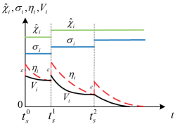
Figure 1: One possible variation of $\hat{\chi}_{i},\sigma_{i},\eta_{i},V_{i}$. $\hat{\chi}_{i},\sigma_{i}$ will keep constant when $V_{i}\leq\eta_{i}$. As long as the event $V_{i}>\eta_{i}$ occurs, the switching will happen and the parameters $\hat{\chi}_{i},\sigma_{i}$ will be updated. Then, $\eta_{i}$ is reset to make $V_{i}<\eta_{i}$ and the previous procedures will be repeated. (For simplicity, $\hat{\Theta}_{i}$ and other variables are not shown in this figure.)

Remark 7

(New supervisory functions) In order to deal with the unstructured uncertainties $h_{i}(\overline{x}_{i}),f_{i}(\overline{x}_{i})$ in each channel of the system (1). The proposed virtual/real control effort $x_{i+1}^{*}$ in (6) or (8) contains adaptive parameters $\hat{\chi}_{i},\hat{\Theta}_{i}$ for $i=1,2,...,n$. Therefore, to guarantee the stability, we need to successively show the boundedness of the parameters $\hat{\chi}_{i},\hat{\Theta}_{i}$ and state $x_{i}$ for $i=1,2,...,n$. This makes the logic-based switching rule in the existing works invalid, where the adaptive parameters may only exist in the last control effort $x_{n+1}^{*}=u$ [18]. Hence, we propose the new supervisory functions (20)-(21) to guide the logic-based switching. The new supervisory functions have the following two major differences from the existing methods, which are important for the boundedness of the adaptive parameters:

1) In the existing works [18, 21], the Lyapunov function is compared with a pre-specified time-varying function. However, for (20), the Lyapunov function $V_{i}$ is compared with a dynamic variable $\eta_{i}$ which is determined by the constructed auxiliary system (21). It relies on the current state information.

2) In [18], only one single supervisory function is used to guide the switching for the adaptive parameters. Yet, in our case, we have used $n$ different supervisory functions $\mathcal{S}_{i}(t)$ to guide the switching for the adaptive parameters in every virtual control effort $x_{i+1}^{*}$.

Note that the new supervisory functions and switching barrier Lyapunov function explained in Remark 5 make the the proposed method has some substantial differences with the existing methods, $e.g.$, [18, 21] and [29]. This is reflected in the stability analysis in Section 3.3, where we propose a new 3-Claims procedure to show the finite time stability.   □

III-C Main result and stability analysis

Based on the analysis in Sections 3.1 and 3.2, we have the following main result.

Theorem 1

Consider the nonlinear system in (1). Then, the controller (5)-(8) with Algorithm 1 can guarantee that:

1) All the signals in the closed-loop system are bounded for $\forall t\in[0,+\infty)$, and;

2) All the states will converge to zero in finite time.

The proof for the above result will be presented in this subsection. According to Remark 6, we can define a switching time sequence $\{0=t_{s}^{0}<t_{s}^{1}<...<t_{s}^{m}<...\leq+\infty\}$ such that

$$t_{s}^{m+1}=\inf\{t|t\geq t_{s}^{m},\mathcal{S}_{i}(t)>0,i\in\{1,2,...,n\}\}.$$ (24)

During time interval $[t_{s}^{m},t_{s}^{m+1})$, the supervisory function satisfies $\mathcal{S}_{i}(t)=V_{i}(\overline{x}_{i},t)-\eta_{i}(t)\leq 0$ for $\forall i=1,2,...,n$. Meanwhile, $\sigma_{i},\hat{\Theta}_{i},\hat{\chi}_{i}(i=1,2,...,n)$ are all constants on $[t_{s}^{m},t_{s}^{m+1})$, i.e., $\sigma_{i}(t)=\sigma_{i}(t_{s}^{m})$, $\hat{\Theta}_{i}(t)=\hat{\Theta}_{i}(t_{s}^{m})$, $\hat{\chi}_{i}(t)=\hat{\chi}_{i}(t_{s}^{m})$ for $\forall t\in[t_{s}^{m},t_{s}^{m+1})$.

The proof will be obtained by proving the following three claims, i.e., Claims 1a, 1b and 1c. Claim 1a tries to show the boundedness of signals in the system if the number of switchings is finite. Next, Claim 1b attempts to show the number of switchings is indeed finite. Finally, Claim 1c proves the finite time stability.

Claim 1a. For any finite integer $m$, we have

1) The closed loop nonlinear system admits continuous solution $\overline{x}_{n}(t)$ on $[t_{s}^{0},t_{s}^{m+1})$;

2) There exists a positive constant $\delta_{i}^{m}$ such that $|s_{i}(t)|\leq\hat{\chi}_{i}(t_{s}^{m})-\delta_{i}^{m}$ for $\forall i=1,2,...,n$ on $[t_{s}^{m},t_{s}^{m+1})$;

3) All the signals in the system are bounded on $[t_{s}^{m},t_{s}^{m+1})$.

Proof:

According to Algorithm 1 and Remark 6, we know during each time interval $[t_{s}^{m},t_{s}^{m+1})$, the initial condition satisfies $|s_{i}(t_{s}^{m})|<\hat{\chi}_{i}(t_{s}^{m})$ and the barrier $\hat{\chi}_{i}$ remains to be constant. Hence, (10) and (15) become traditional barrier Lyapunov functions on each $[t_{s}^{m},t_{s}^{m+1})$. Therefore, according to the theory of barrier Lyapunov functions [28] and the fact that $V_{i}(\overline{x}_{i},t)\leq\eta_{i}(t)$ on each $[t_{s}^{m},t_{s}^{m+1})$, we can show the virtual control error $s_{i}(t)$ is constrained for each $[t_{s}^{m},t_{s}^{m+1})$, $i.e.$, $|s_{i}(t)|\leq\hat{\chi}_{i}(t_{s}^{m})-\delta_{i}^{m}(i=1,2,...,n)$ for $\forall t\in[t_{s}^{m},t_{s}^{m+1})$. Detail proofs are put in Appendix B. ∎

Claim 1b. 1) The number of switchings is finite;

2) The closed loop nonlinear system admits continuous solution $\overline{x}_{n}(t)$ on $[0,+\infty)$;

3) All the signals in the system are bounded on $[0,+\infty)$.

Proof:

Note that from Remark 6 and Claim 1a, we know during each time interval $[t_{s}^{m},t_{s}^{m+1})$, the adaptive paramters keep constant, and $|s_{i}(t)|<\hat{\chi}_{i}(t_{s}^{m})=\hat{\chi}_{i}(t)(i=1,...,n)$ with $t\in[t_{s}^{m},t_{s}^{m+1})$. Thus, $V_{i}\geq 0(i=1,...,n)$ by (10) and Proposition 2. Meanwhile, the propositions in Section 3.1 are all valid for each $[t_{s}^{m},t_{s}^{m+1})$. Keeping this in mind, we will first prove the number of switchings is finite. The proof is divided into the following steps. These steps correspond to the $n$ steps Lyapunov functions analysis in Section 3.1.

Step 1. We will prove $\hat{\chi}_{1},\hat{\Theta}_{1}$ have finite numbers of switchings.

1) Show $\hat{\chi}_{1}(t)$ does not switch on $[t_{s}^{0},t_{s}^{m+1})$.

According to Claim 1a, we know $|s_{1}(t)|\leq\hat{\chi}_{1}(t_{s}^{m})-\delta_{1}^{m}$ on $[t_{s}^{m},t_{s}^{m+1})$ for any finite integer $m$, and $s_{1}(t)=x_{1}(t)$ is continuous on $[t_{s}^{0},t_{s}^{m+1})$. Then, according to Algorithm 1-4) in Switching logic, $\hat{\chi}_{1}$ will not be updated on $[t_{s}^{0},t_{s}^{m+1})$ since $s_{1}(t)$ will never transgress the barrier $\hat{\chi}_{1}(t_{s}^{0})$.

2) Show $\hat{\Theta}_{1}(t)$ has a finite number of switchings.

This is proved by contradiction. If this is not true, then $\hat{\Theta}_{1}$ will switch infinite times.

From Claim 1a and the fact that $\hat{\chi}_{1}(t)=\hat{\chi}_{1}(t_{s}^{0})$ with $t\in[t_{s}^{0},t_{s}^{m+1})$, we have $|s_{1}(t)|=|x_{1}(t)|<\hat{\chi}_{1}(t_{s}^{0})$ is bounded on $[t_{s}^{0},t_{s}^{m+1})$. It follows that on $[t_{s}^{0},t_{s}^{m+1})$, the unstructured uncertainties $h_{1}(x_{1})$ and $F_{1}(x_{1},\hat{\chi}_{1})$ in (11) satisfy

$$|h_{1}(x_{1})|\geq\underline{h}_{1}>0,$$

$$0\leq F_{1}(x_{1},\hat{\chi}_{1})\leq\overline{F}_{1}$$

where $\underline{h}_{1},\overline{F}_{1}$ are unknown constants irrelevant with the number of switchings $m$.

Then, from the tuning rule (9) and the assumption of infinite switchings, we can conclude that there exists a sufficiently large finite integer $m_{1}$ such that at switching time $t_{s}^{m_{1}}$, we have

$$\mathrm{sgn}(\hat{\Theta}_{1}(t_{s}^{m_{1}})) =\mathrm{sgn}(h_{1}(x_{1})),$$

$$-h_{1}K_{1}\hat{\Theta}_{1}(t_{s}^{m_{1}}) \leq-\underline{h}_{1}K_{1}|\hat{\Theta}_{1}(t_{s}^{m_{1}})|<0,$$

$$F_{1}(x_{1},\hat{\chi}_{1})-h_{1}\hat{\Theta}_{1}(t_{s}^{m_{1}}) \leq\overline{F}_{1}-\underline{h}_{1}|\hat{\Theta}_{1}(t_{s}^{m_{1}})|<0$$

This implies that at switching time $t_{s}^{m_{1}}$, (11) will become

$$\dot{V}_{1}\leq -a_{1}V_{1}^{\frac{1+\alpha}{2}}-Q_{1}s_{1}^{1+\alpha}+c_{12}s_{2}^{1+\alpha}$$ (25)

with $a_{1},Q_{1}$ defined in (21).

On the other hand, the auxiliary variable $\eta_{1}(t)$ in (21) satisfies

$$\dot{\eta}_{1}= -a_{1}\eta_{1}^{\frac{1+\alpha}{2}}-Q_{1}s_{1}^{1+\alpha}+c_{12}s_{2}^{1+\alpha}$$ (26)

where $\eta_{1}(t_{s}^{m_{1}})\geq V_{1}(x_{1}(t_{s}^{m_{1}}),t_{s}^{m_{1}})$ according to Algorithm 1-4)-c) in Switching logic.

From Lemma 4 and (25)-(26), we know $V_{1}(x_{1}(t),t)\leq\eta_{1}(t)$ will hold on $[t_{s}^{m_{1}},t_{s}^{m+1})$ for any $m+1>m_{1}$ without resetting $\eta_{1}(t)$. This means that $\hat{\Theta}_{1}$ will not be updated after $t_{s}^{m_{1}}$ which contradicts the fact that $\hat{\Theta}_{1}$ has an infinite number of switchings.

Step 2. We will prove $\hat{\chi}_{2},\hat{\Theta}_{2}$ have finite numbers of switchings.

The proof will be conducted on $[t_{s}^{m_{1}},t_{s}^{m+1})$ where $t_{s}^{m_{1}}$ denotes the time instant when $\hat{\chi}_{1},\hat{\Theta}_{1}$ stop switching and keep constant.

1) Show $\hat{\chi}_{2}(t)$ does not switch on $[t_{s}^{m_{1}},t_{s}^{m+1})$.

Note that $\hat{\Theta}_{1}$ is not updated on $[t_{s}^{m_{1}},t_{s}^{m+1})$. Meanwhile, according to Claim 1a, we know $x_{2}$ is continuous on $[t_{s}^{m_{1}},t_{s}^{m+1})$. Then, by (6) and (7), $s_{2}$ is continuous on $[t_{s}^{m_{1}},t_{s}^{m+1})$. Also by Claim 1a, we have $|s_{2}(t)|\leq\hat{\chi}_{2}(t_{s}^{m})-\delta_{2}^{m}$ on $[t_{s}^{m},t_{s}^{m+1})$ for any finite integer $m$. Therefore, according to Algorithm 1-4) in Switching logic, $\hat{\chi}_{2}$ will not be updated on $[t_{s}^{m_{1}},t_{s}^{m+1})$ since $s_{2}(t)$ will never transgress the barrier $\hat{\chi}_{2}(t_{s}^{m_{1}})$.

2) Show $\hat{\Theta}_{2}(t)$ has a finite number of switchings.

This is proved by contradiction. We suppose $\hat{\Theta}_{2}(t)$ will switch infinite times.

First, since $\hat{\chi}_{2}$ is not updated on $[t_{s}^{m_{1}},t_{s}^{m+1})$, we have $|s_{2}(t)|<\hat{\chi}_{2}(t_{s}^{m_{1}})$ with $t\in[t_{s}^{m_{1}},t_{s}^{m+1})$ by Claim 1a. In addition, from Claim 1a, we know $\hat{\chi}_{2}(t_{s}^{m_{1}})$ is bounded.

Using (26) in Step 1 we know $\eta_{1}$ satisfies

$$\dot{\eta}_{1}= -a_{1}\eta_{1}^{\frac{1+\alpha}{2}}-Q_{1}s_{1}^{1+\alpha}+c_{12}s_{2}^{1+\alpha}$$

$$\leq -a_{1}\eta_{1}^{\frac{1+\alpha}{2}}+c_{12}\hat{\chi}_{2}^{1+\alpha}(t_{s}^{m_{1}})$$

on $[t_{s}^{m_{1}},t_{s}^{m+1})$.

Therefore, it can be concluded that $0\leq V_{1}\leq\eta_{1}$ is bounded by a constant irrelevant with $m$ (see Corollary 1 in [33]). Then, from the barrier Lyapunov function (10), we know $|s_{1}(t)|=|x_{1}(t)|\leq\hat{\chi}_{1}(t_{s}^{0})-\delta_{1}$ with a positive constant $\delta_{1}$ irrelevant with $m$. Also from (6) and (7), we know $x_{2}^{*},x_{2}$ are both bounded by constants irrelevant with $m$.

Hence, we conclude that on $[t_{s}^{m_{1}},t_{s}^{m+1})$, $h_{2}(\overline{x}_{2})$ and $F_{2}(\overline{x}_{2},\hat{\Theta}_{1},\hat{\chi}_{1})$ in (17) satisfy

$$|h_{2}(\overline{x}_{2})|\geq\underline{h}_{2}>0,$$

$$0\leq F_{2}(\overline{x}_{2},\hat{\Theta}_{1},\overline{\hat{\chi}}_{2})\leq\overline{F}_{2}$$

where $\underline{h}_{2},\overline{F}_{2}$ are positive constants irrelevant with $m$. Here, we also use the fact that $\hat{\chi}_{1},\hat{\chi}_{2},\hat{\Theta}_{1}$ are constants on $[t_{s}^{m_{1}},t_{s}^{m+1})$.

Then, from tuning rule (9), there exists a finite integer $m_{2}\geq m_{1}$ such that at switching time $t_{s}^{m_{2}}$, we have

$$\mathrm{sgn}(\hat{\Theta}_{2}(t_{s}^{m_{2}})) =\mathrm{sgn}(h_{2}(\overline{x}_{2})),$$

$$-h_{2}K_{2}\hat{\Theta}_{2}(t_{s}^{m_{2}}) \leq-\underline{h}_{2}K_{2}|\hat{\Theta}_{2}(t_{s}^{m_{2}})|<0,$$

$$F_{2}(\overline{x}_{2},\hat{\Theta}_{1},\overline{\hat{\chi}}_{2})-h_{2}\hat{\Theta}_{2}(t_{s}^{m_{2}}) \leq\overline{F}_{2}-\underline{h}_{2}|\hat{\Theta}_{2}(t_{s}^{m_{2}})|<0$$

This implies that (17) will become

$$\dot{V}_{2}\leq -a_{2}V_{2}^{\frac{1+\alpha}{2}}-Q_{2}s_{2}^{1+\alpha}+c_{21}s_{1}^{1+\alpha}+c_{23}s_{3}^{1+\alpha}$$ (27)

at switching time $t_{s}^{m_{2}}$ with $a_{2},Q_{2}$ defined in (21).

On the other hand, the auxiliary variable $\eta_{2}(t)$ in (21) satisfies

$$\dot{\eta}_{2}= -a_{2}\eta_{2}^{\frac{1+\alpha}{2}}-Q_{2}s_{2}^{1+\alpha}+c_{21}s_{1}^{1+\alpha}+c_{23}s_{3}^{1+\alpha}$$ (28)

where $\eta_{2}(t_{s}^{m_{2}})\geq V(\overline{x}_{2}(t_{s}^{m_{2}}),t_{s}^{m_{2}})$ according to Algorithm 1-5) in Switching logic.

From Lemma 4 and (27)-(28), we know $V_{2}(\overline{x}_{2}(t),t)\leq\eta_{2}(t)$ will hold on $[t_{s}^{m_{2}},t_{s}^{m+1})$ for any $m+1>m_{2}$ without resetting. This means that $\hat{\Theta}_{2}$ will not be updated after $t_{s}^{m_{2}}$ which contradicts the fact that $\hat{\Theta}_{2}$ has an infinite number of proof.

Step i($3\leq i\leq n$). By repeating the above procedures, we can show all the parameters $\hat{\Theta}_{i},\hat{\chi}_{i}(i=1,2,...,n)$ have finite numbers of switchings. Statement 1) in Claim 1b is proved

Next, for Statements 2)-3) in Claim 1b, according to Claim 1a, they hold naturally when the number of switchings is finite. In fact, there must exist a finite integer $m_{n}$ such that the switching time $t_{s}^{m_{n}+1}=+\infty$. The proof is completed. ∎

Claim 1c. All the states will converge to zero in finite time.

Proof:

From Claim 1a, we know $|s_{i}(t)|<\hat{\chi}_{i}(t_{s}^{m})=\hat{\chi}_{i}(t)(i=1,...,n)$ for $\forall t\in[t_{s}^{m},t_{s}^{m+1})$. Then, we have $V_{i}\geq 0(i=1,...,n)$ by (10), (15) and Proposition 2. From Claim 1b, we know the number of switchings is finite. This implies that there exists a finite switching time $t_{s}^{m_{n}}$ where $m_{n}$ is a finite integer and $t_{s}^{m_{n}+1}=+\infty$. When $t\in[t_{s}^{m_{n}},t_{s}^{m_{n}+1})=[t_{s}^{m_{n}},+\infty)$, $0\leq V_{i}\leq\eta_{i}$ holds for $\forall i\in\{1,2,...,n\}$ without resetting $\eta_{i}$. Then, on $[t_{s}^{m_{n}},+\infty)$, by (21)-(23) we have

$$\dot{\overline{\eta}}\leq-a^{\prime}\overline{\eta}^{\gamma}$$

where $a^{\prime}>0$ is a positive parameter, $\gamma\triangleq\frac{1+\alpha}{2}\in(0,1)$.

Therefore, during time interval $[t_{s}^{m_{n}},+\infty)$, we have

$${\color[rgb]{0,0,0}{\color[rgb]{0,0,0}0\leq}} {\color[rgb]{0,0,0}{\color[rgb]{0,0,0}\sum_{i=1}^{n}V_{i}\leq\overline{\eta}}}(t)$$

$$\leq [\overline{\eta}^{1-\gamma}(t_{s}^{m_{n}})-a^{\prime}(1-\gamma)(t-t_{s}^{m_{n}})]^{\frac{1}{1-\gamma}}.$$

Note that by Claim 1b, all the signals including $\overline{\eta}(t_{s}^{m_{n}})$ are bounded on $[0,+\infty)$. Hence, we can conclude that after finite time $t_{s}^{m_{n}}+\frac{\eta^{1-\gamma}(t_{s}^{m_{n}})}{a^{\prime}(1-\gamma)}$, $\overline{\eta}$ and $V_{i}(i=1,2,...,n)$ will converge to zero. By (5)-(8), (10), (15) and (16), we know $s_{1}=x_{1},x_{2}^{*},x_{2},s_{2},x_{3}^{*},x_{3},...,x_{n}$ will also converge to zero in finite time. The proof is completed. ∎

IV Examples

In this section, an illustrative example is presented. Note that some further discussions about convergence speed, control overshoot, controller parameters selection, comparison with existing asymptotic control methods and control of third order nonlinear systems are put in Appendix F in the supplementary file.

Example 1

Given a second order nonlinear system by (1) with $n=2$, we consider the following six cases:

$$\mathrm{Case}\thinspace\mathrm{A}: h_{1}=1,h_{2}=0.8,f_{1}=\overline{f}_{1},f_{2}=\overline{f}_{2};$$

$$\mathrm{Case}\thinspace\mathrm{B}: h_{1}=1,h_{2}=-0.8,f_{1}=\overline{f}_{1},f_{2}=\overline{f}_{2};$$

$$\mathrm{Case}\thinspace\mathrm{C}: h_{1}=1,h_{2}=0.8,f_{1}=5\overline{f}_{1},f_{2}=5\overline{f}_{2};$$

$$\mathrm{Case}\thinspace\mathrm{D}: h_{1}=-1,h_{2}=0.8,f_{1}=\overline{f}_{1},f_{2}=\overline{f}_{2};$$

$$\mathrm{Case}\thinspace\mathrm{E}: h_{1}=-1,h_{2}=-0.8,f_{1}=\overline{f}_{1},f_{2}=\overline{f}_{2};$$

$$\mathrm{Case}\thinspace\mathrm{F}: h_{1}=-1,h_{2}=0.8,f_{1}=f_{1}^{*},f_{2}=f_{2}^{*}$$

where $\overline{f}_{1}\triangleq 0.1\sin(x_{1})x_{1}$; $\overline{f}_{2}\triangleq-4.9\sin(x_{1})+0.05\sin(x_{1})e^{-x_{2}}+0.1\sin(x_{2})x_{2}^{2}.$ $f_{1}^{*}\triangleq-3x_{1}^{2}/2-x_{1}^{3}/2$ and $f_{2}^{*}\triangleq 0.1\sin(x_{2})$. Case A is the nominal case. It can be used to describe the dynamics of a single link robot manipulator [34]. Other five situations represent the variation of control directions and modeling uncertainties. Specifically, Case F indicates that the whole system has been changed into another form. The initial conditions are $x_{1}(0)=0.1,x_{2}(0)=0.2.$ For the controller design, we assume $h_{1},h_{2},f_{1},f_{2}$ are all unknown.

1) Effectiveness of the logic-based switching

The controller is designed by (5)-(8). The controller parameters are set as: $K_{1}=U_{1}=K_{2}=U_{2}=1$, $\alpha=41/49$, $\hat{\chi}_{1}=\hat{\chi}_{2}(0)=2$. $\theta_{1}(0)=\theta_{2}(0)=0.1$ and for $\sigma_{i}(t)\geq 1(i=1,2)$, we have $\theta_{i}(\sigma_{i})=(-1)^{\sigma_{i}(t)}(\iota_{i1}+\iota_{i2}\sigma_{i})$ where $\iota_{i1}=\iota_{i2}=1.$ $\hat{\Theta}_{1},\hat{\Theta}_{2}\text{,$\hat{\chi}_{1}$,$\hat{\chi}_{2}$ }$ are updated by Algorithm 1 with $\varsigma=4,\varepsilon=0.01$, $a_{1}=a_{2}=0.2,$ $Q_{1}=Q_{2}=c_{11}=c_{21}=1$. The control performance is shown in Fig. 5. It can be seen that both states converge to zero in a very short time for the above six situations. This implies that the finite time stability has been achieved despite multiple unknown control directions and unstructured uncertainties.

Next, set $\hat{\chi}_{2}(0)=0.8,\hat{\chi}_{1}(0)=2$. The variations of $s_{i},\hat{\Theta}_{i},\hat{\chi}_{i}(i=1,2)$ are shown in Fig. 6. Note that $s_{1}$ is constrained into the tube $[-2,2]$. This shows the validity of the barrier Lyapunov function $V_{1}$ in (10). Also we can see $s_{2}$ is constrained into the tube $[-0.8,0.8]$ during time interval $[0,1.35)$ and is larger than $\hat{\chi}_{2}(0)=0.8$ at time instant $1.35s$. Therefore, $\hat{\chi}_{2}$ jumps to $4.8$ to contain $s_{2}$ in the later time. The reason for $s_{2}$ jumping outside $0.8$ is that $\hat{\Theta}_{1}$ is updated at $1.35s$. Note that though $s_{2}$ transgresses over the barrier $\hat{\chi}_{2}(0)=0.8$, $s_{1},s_{2}$ still can converge to zero in finite time. All these show the effectiveness of the switching barrier Lyapunov function.

2) Comparision with Nussbaum-gain method

Consider the system described by Example 1. Given a finite time controller by (5)-(8) with the same parameters in Example 1, and another controller designed by Nussbaum-gain technique:

$$u =\mathcal{N}_{2}(\xi_{2})v_{2},$$

$$v_{2} =K_{2}s_{2}+\frac{U_{2}s_{2}}{\hat{\chi}_{2}^{2}-s_{2}^{2}},$$

$$\dot{\xi}_{2} =\frac{s_{2}v_{2}}{\hat{\chi}_{2}^{2}-s_{2}^{2}}$$

where

$$s_{2} =x_{2}-x_{2}^{*},$$

$$x_{2}^{*} =\mathcal{N}_{1}(\xi_{1})v_{1},$$

$$v_{1} =K_{1}s_{1}+\frac{U_{1}s_{1}}{\hat{\chi}_{1}^{2}-s_{1}^{2}},$$

$$\dot{\xi}_{1} =\frac{s_{1}v_{1}}{\hat{\chi}_{1}^{2}-s_{1}^{2}}.$$

$\mathcal{N}_{i}(\xi_{i})(i=1,2)$ are Nussbaum functions such that $\mathcal{N}_{i}(\xi_{i})=\xi_{i}^{2}\cos(\xi_{i}).$ $K_{1},U_{1},K_{2},U_{2},\hat{\chi}_{1},\hat{\chi}_{2}$ are positive design parameters. The parameters are set as: $K_{1}=U_{1}=1,K_{2}=U_{2}=4,\hat{\chi}_{1}=2,\hat{\chi}_{2}=1$. Using these parameters, a satisfactory control performance can be obtained in the nominal case. This controller is a variation of the method in [15], which adapts to the unstructured uncertainties.

Fig. 2 shows the state trajectories and variation of control effort in Case A. We can see that the finite time control method has a faster convergence speed and higher precision than Nussbaum-gain method. In fact, the states by finite time control is around $3.75\times 10^{-5}$ after $6.5s$, while states by Nussbaum-gain method is $0.01$. Moreover, the proposed method has a smaller overshoot and control effort than Nussbaum-gain method. The reason for this may be that the proposed method can find a proper control direction quickly by switching logic.

Next, with the same controller parameters, we consider the control performance in Cases B-F. Fig. 3 shows the state trajectories in Cases B and C. We can see that in both cases, the proposed method has a superior performance with smaller overshoot and faster convergence rate. Fig. 4 demonstrates the state trajectories in Cases D and E, it can be seen that control performance of Nussbaum-gain method deteriorates a lot. For Case F, the Nussbaum-gain method has become highly unstable. All these show the stronger robustness of the proposed method.

Example 2

To further verify the validity of the proposed method, an experiment is conducted. The experimental platform is shown in Fig. LABEL:fig:ex12. It involves the following three main parts: (1) A DC brush motor with an encoder; (2) A STM32F407 control board. The control board samples the actual velocity every millisecond, which aims to realize the velocity closed-loop control. (3) A H bridge drive circuit board. We assume that we do not know the control direction. The controller parameters are set as: $K_{1}=10,K_{2}=12,\theta_{1}(0)=0.5$ and for $\sigma_{1}(t)\geq 1$, we have $\theta_{1}(\sigma_{1})=(-1)^{\sigma_{1}(t)}(\iota_{11}+\iota_{12}\sigma_{1})$, where $\iota_{11}=\iota_{12}=1$. The experimental results are shown in Fig. LABEL:fig:ex3-LABEL:fig:ex4. Fig. LABEL:fig:ex3 shows the tracking performance. Fig. LABEL:fig:ex4 shows the variations of $V,\eta$ and control input. We can see that the system output can track the reference signal accurately. The control parameters can be adaptively adjusted to identify the system control direction. All these show the validity of the proposed method.

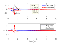
Figure 2: Control performance comparison for Case A.

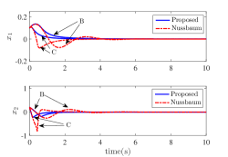
Figure 3: Control performance comparison for Cases B and C.

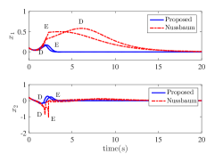
Figure 4: Control performance comparison for Cases D and E.

Figure 5: Control performance for second order system.

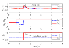
Figure 6: Variations of $s_{i},\hat{\Theta}_{i},\hat{\chi}_{i}(i=1,2)$. It can be seen that $|s_{2}|$ is constrained in the barrier $\hat{\chi}_{2}(t)=0.8$ during time interval $[0,1.35)$ and jump outside the barrier $\hat{\chi}_{2}(t)$ at time instant $1.35s$ due to $\hat{\Theta}_{1}$ is updated. Then, by the proposed method, $\hat{\chi}_{2}$ will switch to $4.8$ to contain $s_{2}$ in the later time to guarantee the finite time stability.

V Conclusions

In this paper, two kinds of logic-based switching adaptive controllers are proposed. The finite time stability can be guaranteed for the nonlinear systems suffering from multiple unknown control directions and unstructured uncertainties. Future work will be focused on extending the presented design approach to general hybrid systems.

Appendix A Proof of Lemma 4

Proof:

This is a variation of Comparison Principle [33]. Subtracting (3) from (4), we have:

$$\dot{e}(t)\leq-a[y^{\gamma}(t)-x^{\gamma}(t)]$$ (29)

where $e(t)\triangleq y(t)-x(t).$ Then, we only need to prove $e(t)\leq 0$ for $\forall t\in[t_{0},t_{1})$. In fact, if this is not true, there must exist a time instant $t^{*}\in[t_{0},+\infty)$ such that $e(t^{*})>0$. Since $e(t_{0})=y(t_{0})-y(t_{0})-\varepsilon=-\varepsilon\leq 0$, we can conclude that there exists a time interval $[\tau_{1},\tau_{2}]\subseteq[t_{0},t^{*}]$ such that $e(\tau_{1})=0$, $e(t)>0$ for $\forall t\in(\tau_{1},\tau_{2}]$. By Mean Value Theorem, there exists a time instant $\tau_{3}\in[\tau_{1},\tau_{2}]$ such that $e(\tau_{3})>0$ and $\dot{e}(\tau_{3})>0$. However, this contradicts (29). It completes the proof. ∎

Appendix B Proof of Claim 1a

The proof is divided into two parts. For the first part, we will show Claim 1a holds with $m=0$. The second part will show Claim 1a is true for any finite integer $m$.

Part I

We will prove the following claim.

Claim 1a^′. Suppose $|s_{i}(t_{s}^{0})|<\hat{\chi}_{i}(t_{s}^{0})$ and $\eta_{i}(t_{s}^{0})>V_{i}(\overline{x}_{i}(t_{s}^{0}),t_{s}^{0})$ for $\forall i=1,2,...,n$, then we have

1) The considered closed loop nonlinear system admits continuous solution $\overline{x}_{n}(t)$ on $[t_{s}^{0},t_{s}^{1})$;

2) There exists a positive constant $\delta_{i}^{0}$ such that $|s_{i}(t)|\leq\hat{\chi}_{i}(t_{s}^{0})-\delta_{i}^{0}$ for $\forall i=1,2,...,n$ on $[t_{s}^{0},t_{s}^{1})$;

3) All the signals in the system are bounded on $[t_{s}^{0},t_{s}^{1})$.

Proof:

The proof is divided into following phases.

1) Prove that the closed loop system admits continuous solution $\overline{x}_{n}(t)$ on $[t_{s}^{0},t^{*})$ with $|s_{i}(t)|<\hat{\chi}_{i}(t_{s}^{0})(i=1,2,...,n)$ and $t_{s}^{0}<t^{*}\leq t_{s}^{1}$.

According to the Initialization in Algorithm 1, we know $|s_{i}(t_{s}^{0})|<\hat{\chi}_{i}(t_{s}^{0})$ and $\eta_{i}(t_{s}^{0})>V_{i}(\overline{x}_{i}(t_{s}^{0}),t_{s}^{0})$. Meanwhile, nonlinear functions $h_{i}(\overline{x}_{i}),f_{i}(\overline{x}_{i})$ in (1) are continuously differentiable and adaptive parameters $\hat{\chi}_{i},\hat{\Theta}_{i}$ are constants on $[t_{s}^{0},t_{s}^{1})$. Then, according to [28] and [35], we know the above statement is true.

2) Prove $t^{*}$ can be extended to $t_{s}^{1}$. That is the closed loop system admits continuous solution $\overline{x}_{n}(t)$ on $[t_{s}^{0},t_{s}^{1})$ with $|s_{i}(t)|<\hat{\chi}_{i}(t_{s}^{0})(i=1,2,...,n)$.

This is proved by contradiction. If this is not true, then $t^{*}<t_{s}^{1}$ and there exists an integer $i^{\prime}\in\{1,2,...,n\}$ such that as $t\rightarrow t^{*}$, $|s_{i^{\prime}}(t)|\rightarrow\hat{\chi}_{i^{\prime}}(t_{s}^{0})$. Meanwhile, $|s_{i}(t)|<\hat{\chi}_{i}(t_{s}^{0})$ for $\forall i=1,2,...,n$ on $[t_{s}^{0},t^{*})$.

Note that from (23), we know $\dot{\overline{\eta}}\leq-a^{\prime}\overline{\eta}^{\frac{1+\alpha}{2}}\leq 0$ where we have used the fact that $\eta_{i}\geq V_{i}\geq 0(i=1,...,n)$ on $[t_{s}^{0},t^{*})$. This means that all the Lyapunov functions $V_{i}(i=1,...,n)$ are bounded. Next, analysis will be taken on each step in the controller design to seek a contradiction.

Step 1. Since $V_{1}$ is bounded, from (10) we conclude that there exists a positive constant $\delta_{1}^{0}$ such that $|s_{1}|\leq\hat{\chi}_{1}(t_{s}^{0})-\delta_{1}^{0}$. Using (6) and (7), we know $x_{2}^{*},x_{2}$ are both bounded.

Step i($2\leq i\leq n$). Due to $x_{i}^{*},V_{i}$ are bounded, from Proposition 2 we know there exists a positive constant $\delta_{i}^{0}$ such that $|s_{i}|\leq\hat{\chi}_{i}(t_{s}^{0})-\delta_{i}^{0}$. Using (6)-(8), we conclude that $x_{i+1}^{*},x_{i+1}$ are both bounded with $x_{n+1}\triangleq 0$.

Therefore, we have $|s_{i}|\leq\hat{\chi}_{i}(t_{s}^{0})-\delta_{i}^{0}$ for $i=1,2,...,n$. This contradicts the fact that there exists an integer $i^{\prime}\in\{1,2,...,n\}$ such that when $t\rightarrow t^{*}$, $|s_{i^{\prime}}(t)|\rightarrow\hat{\chi}_{i^{\prime}}(t_{s}^{0})$. Then, we can conclude that the system has continuous solution on $[t_{s}^{0},t_{s}^{1})$ with $|s_{i}(t)|<\hat{\chi}_{i}(t_{s}^{0})$.

3) Prove Claim 1a^′ is true.

This can be proved by following the line of the above procedures and using the fact that $|s_{i}(t)|<\hat{\chi}_{i}(t_{s}^{0})(i=1,2,...,n)$ on $[t_{s}^{0},t_{s}^{1})$. ∎

Part II

We will prove Claim 1a holds for any finite integer $m$.

According to Claim 1a^′, we know the system admits continuous solution on $[t_{s}^{0},t_{s}^{1})$. Then, by Algorithm 1 and Remark 6, it is not hard to show at switching time $t_{s}^{1}$, we have

1) $s_{i}(t_{s}^{1}),\hat{\chi}_{i}(t_{s}^{1}),\eta_{i}(t_{s}^{1}),V_{i}(\overline{x}_{i}(t_{s}^{1}),t_{s}^{1})$ are all bounded for $\forall i=1,2,...,n$;

2) $|s_{i}(t_{s}^{1})|<|\hat{\chi}_{i}(t_{s}^{1})|$ and $\eta_{i}(t_{s}^{1})>V_{i}(\overline{x}_{i}(t_{s}^{1}),t_{s}^{1})$ for $\forall i=1,2,...,n$.

Then, by regarding $t_{s}^{1}$ as a new initial time and repeating the procedures in Claim 1a^′, we can prove Claim 1a holds with $m=1$. Similarily, we can prove the result for any finite $m$. The proof is completed.

References

- [1] Zhao, Z.-L., & Jiang, Z.-P. (2018). Finite-time output feedback stabilization of lower-triangular nonlinear systems. Automatica, 96, 259-269.
- [2] Li, H., Zhao, S., He, W., & Lu, R. (2019). Adaptive finite-time tracking control of full state constrained nonlinear systems with dead-zone. Automatica, 100, 99-107.
- [3] Yu, J., Shi, P., & Zhao, L. (2018). Finite-time command filtered backstepping control for a class of nonlinear systems. Automatica, 92, 173-180.
- [4] Chen, C., & Sun, Z. (2020). A unified approach to finite-time stabilization of high-order nonlinear systems with an asymmetric output constraint. Automatica, 111, 108581.
- [5] Cao, Y., Ren, W., Casbeer, D., & Schumacher, C. (2016). Finite-time connectivity-preserving consensus of networked nonlinear agents with unknown Lipschitz terms. IEEE Transactions on Automatic Control, 61(6), 1700-1705.
- [6] Zhao, G.-H., Li, J.-C., & Liu, S.-J. (2018). Finite-time stabilization of weak solutions for a class of non-local Lipschitzian stochastic nonlinear systems with inverse dynamics. Automatica, 98, 285-295.
- [7] Song, Y., Wang, Y., Holloway, J., Krstic, M. (2017). Time-varying feedback for regulation of normal-form nonlinear systems in prescribed finite time. Automatica, 83, 243-251.
- [8] Lin, H., Chen, K., & Lin, R. (2019). Finite-time formation control of unmanned vehicles using nonlinear sliding mode control with disturbances. International Journal of Innovative Computing, Information and Control, 15(6), 2341-2353.
- [9] Yang, C., Jiang, Y., He, W., Na, Jiang, Li, Z., & Xu, B. (2018). Adaptive parameter estimation and control design for robot manipulators with finite-time convergence. IEEE Transactions on Industrial Electronics, 65(10), 8112-8123.
- [10] Mishra, J., Wang, L., Zhu, Y., Yu, X., & Jalili, M. (2019). A novel mixed cascaded finite-time switching control design for induction motor. IEEE Transactions on Industrial Electronics, 66(2), 1172-1181.
- [11] Zheng, S., & Li, W. (2019). Fuzzy finite time control for switched systems via adding a barrier power integrator. IEEE Transations on Cybernetics, 49(7), 2693-2706.
- [12] Nussbaum, R. D. (1983). Some remarks on a conjecture in parameter adaptive control. Systems & Control Letters, 3, 243-246
- [13] Chen, Z. (2019). Nussbaum functions in adaptive control with time-varying unknown control coefficients. Automatica, 102, 72-79.
- [14] Li, F., & Liu, Y. (2018). Control design with prescribed performance for nonlinear systems with unknown control directions and nonparametric uncertainties. IEEE Transactions on Automatic Control, 63(10), 3573-3580.
- [15] Liu, Y., & Tong, S. (2017). Barrier Lyapunov functions for Nussbaum gain adaptive control of full state constrained nonlinear systems. Automatica, 76, 143-152.
- [16] Yin, S., Gao, H., Qiu, J., & Kaynak, O. (2017). Adaptive fault-tolerant control for nonlinear system with unknown control directions based on fuzzy approximation. IEEE Transactions on Systems, Man, and Cybernetics: Systems, 47(8), 1909-1917.
- [17] Zhang, J.-X., & Yang, G.-H. (2017). Prescribed performance fault-tolerant control of uncertain nonlinear systems with unknown control directions. IEEE Transactions on Automatic Control, 62(12), 6529-6535.
- [18] Chen, W., Wen, C., & Wu, J. (2018). Global exponential/finite-time stability of nonlinear adaptive switching systems with applications in controlling systems with unknown control direction. IEEE Transactions on Automatic Control, 63(8), 2738-2744.
- [19] Wu, J., Chen, W., & Li, J. (2016). Global finite-time adaptive stabilization for nonlinear systems with multiple unknown control directions. Automatica, 69, 298-307.
- [20] Wu, J., Li, J., Zong, G. D., & Chen, W. S. (2017). Global finite-time adaptive stabilization of nonlinearly parameterized systems with multiple unknown control directions. IEEE Transactions on Systems, Man, and Cybernetics: Systems, 47(7), 1405-1414.
- [21] Fu, J., Ma, R., & Chia, T. (2017). Adaptive finite-time stabilization of a class of uncertain nonlinear systems via logic-based switchings. IEEE Transactions on Automatic Control, 62(11), 5998-6001.
- [22] Huang, J., Wen, C., Wang, W., & Song, Y. (2016). Design of adaptive finite-time controllers for nonlinear uncertain systems based on given transient specifications. Automatica, 69, 395-404.
- [23] Huang, S., & Xiang, Z. (2016). Finite-time stabilization of switched stochastic nonlinear systems with mixed odd and even powers. Automatica, 73, 130-137.
- [24] Liu, X., Zhai, D., Li, T., & Zhang, Q. (2019). Fuzzy-approximation adaptive fault-tolerant control for nonlinear pure-feedback systems with unknown control directions and sensor failures. Fuzzy Sets and Systems, 356, 28-43.
- [25] Qian, C., & Lin, W. (2001). Non-Lipschitz continuous stabilizers for nonlinear systems with uncontrollable unstable linearization. Systems & Control Letters. 42(3), 185-200.
- [26] Chen, Z., & Huang, J. (2015). Stabilization and regulation of nonlinear systems: A Robust and adaptive approach. Springer.
- [27] Lin, W., & Gong, Q. (2003). A remark on partial-state feedback stabilization of cascade systems using small gain theorem. IEEE Transactions on Automatic Control, 48(3), 497-500.
- [28] Tee, K. P., Ge, S. S., & Tay, E. H. (2009). Barrier Lyapunov functions for the control of output-constrained nonlinear systems. Automatica, 45(4), 918-927.
- [29] Yu, J., Zhao, L., Yu, H., & Lin, C. (2019). Barrier Lyapunov functions-based command filtered output feedback control for full-state constrained nonlinear systems. Automatica, 105, 71-79.
- [30] Liu, Y., Lu, S., Tong, S., Chen, X., Chen, C. L., & Li, D. (2018). Adaptive control-based Barrier Lyapunov Functions for a class of stochastic nonlinear systems with full state constraints. Automatica, 87, 83-93.
- [31] Huang, C., & Yu, C. (2018). Tuning function design for nonlinear adaptive control systems with multiple unknown control directions. Automatica, 89, 259-265.
- [32] Hespanha, J., Liberzon, D., & Morse, A. (2003). Hysteresis-based switching algorithms for supervisory control of uncertain systems. Automatica, 39(2), 263-272.
- [33] Khalil, H. K. (2002). Nonlinear systems. Third Edition. Prentice-Hall, Inc. Upper Saddle River, NJ.
- [34] Xing, L., Wen, C., Liu, Z., Su, H., & Cai, J. (2017). Adaptive compensation for actuator failures with event-triggered input. Automatica, 85, 129-136.
- [35] Sontag, E. D. (1998). Mathematical control theory. In Texts in Applied Mathematics: Vol. 6. Deterministic finite-dimensional systems (2nd ed.). New York: Springer-Verlag.