How Much and When Do We Need Higher-order Information in Hypergraphs? A Case Study on Hyperedge Prediction

Abstract.

Hypergraphs provide a natural way of representing group relations, whose complexity motivates an extensive array of prior work to adopt some form of abstraction and simplification of higher-order interactions. However, the following question has yet to be addressed: How much abstraction of group interactions is sufficient in solving a hypergraph task, and how different such results become across datasets? This question, if properly answered, provides a useful engineering guideline on how to trade off between complexity and accuracy of solving a downstream task. To this end, we propose a method of incrementally representing group interactions using a notion of $n$-projected graph whose accumulation contains information on up to $n$-way interactions, and quantify the accuracy of solving a task as $n$ grows for various datasets. As a downstream task, we consider hyperedge prediction, an extension of link prediction, which is a canonical task for evaluating graph models. Through experiments on 15 real-world datasets, we draw the following messages: (a) Diminishing returns: small $n$ is enough to achieve accuracy comparable with near-perfect approximations, (b) Troubleshooter: as the task becomes more challenging, larger $n$ brings more benefit, and (c) Irreducibility: datasets whose pairwise interactions do not tell much about higher-order interactions lose much accuracy when reduced to pairwise abstractions.

1. Introduction

Graphs cover a wide range of applications, but there are domains in which an ordinary graph would fail to capture the relations of entities. Consider a research community, where authors publish papers in groups of more than two. It would involve information loss to represent such groups of collaborators as just pairwise edges as in an ordinary graph. Such interactions are effectively captured by hyperedges, an extended notion of edges that join an arbitrary number of entities. Graphs with hyperedges, referred to as hypergraphs, are everywhere in our offline/online networks. People gather in groups (Sinha et al., 2015), biological phenomena are caused by joint protein interactions (Navlakha and Kingsford, 2010), and web posts contain tags (Zhang, 2019; Ofli et al., 2017).

One of the critical issues in playing with hypergraphs is how to process, simplify, and represent higher-order interactions for a given task. One may make a highly abstract representation of complex multi-way interactions, e.g., (Zhang et al., 2018; Yadati et al., 2018b; Benson et al., 2018a; Xu et al., 2013; Li et al., 2013), while others may use the original hypergraph as it is, e.g., (Sharma et al., 2014; Arya and Worring, 2018; Huang et al., 2015b; Yadati et al., 2018a; Feng et al., 2019; Benson et al., 2018b). Despite the recent advances in processing units and memory devices for high-performance data processing, it is still daunting and computationally intractable to maintain whole group interactions in large-scale hypergraphs and use them for solving a given task.

We are motivated by such a reality and ask the following question: How much abstraction of group interactions is sufficient in solving a given graph task, and how different such results become across datasets that vary in scale, entities, and pattern of interactions? The answers to this question would give us useful engineering guidelines on how to appropriately trade off between complexity in representation of higher-order group interactions and accuracy of solving the task. In seeking to answer this question, we may find a new method that outperforms existing algorithms in literature while maintaining computational tractability. In this paper, we consider the hyperedge prediction task, which is a hypergraph extension of link prediction. Link prediction is a widely accepted means of assessing the validity of graph models (Liben-Nowell and Kleinberg, 2007; Lü and Zhou, 2011; Grover and Leskovec, 2016; Zhou et al., 2017; Santolini and Barabási, 2018; You et al., 2019; Grover et al., 2019).

As an important device to answer our question by solving the hyperedge prediction task, we introduce the $n$-projected graph, $G_{n}$, $n=2,3,\ldots$ for a given hypergraph $G$. This is a modified version of the original hypergraph $G$ so as to contain $n$-way group interactions. By incrementally stacking $n$-projected graphs, we can represent the original hypergraph with up to $n$-way interactions. As expected, as $n$ grows, we reduce the information loss, but the computational cost for processing increases. The notion of projected graphs is not entirely new as adopted in (Zhang et al., 2018; Yadati et al., 2018b; Benson et al., 2018a; Sharma et al., 2014). However, it has been limited to the pairwise relation, which turns out to be the $2$-projected graph, a special case of the $n$-projected graph. We generalize this pairwise relation to $n$-way interactions in $G_{n}$ to quantify and decompose the degree of interactions, constructed as follows: Each edge in $G_{n}$ is weighted by the number of hyperedges in which the node set of size $n$ have appeared together (see Section 4 for details).

The value of the $n$-projected graph is clear by the following example: Suppose that we want to predict whether four people would collaborate or not in the future. It is useful to know how much each pair has collaborated together as in $2$-projected graph. However, collaboration is often formed because a group of three people, who have collaborated as a group, may recruit a fourth person in the future, where $3$-way interaction becomes valuable.

We conduct experiments using 15 datasets spanning 8 domains provided by (Benson et al., 2018a; Stehlé et al., 2011; Mastrandrea et al., 2015; Yin et al., 2017; Leskovec et al., 2007; Fowler, 2006a, b; Sinha et al., 2015). These datasets are highly heterogeneous in terms of scale, pattern of interactions, and interacting entities, ranging from about 1,000 to 2,500,000 hyperedges. We use logistic regression for prediction, where we utilize the features popularly used in link/hyperedge prediction tasks but generalized for $n$-projected graphs. The prediction results would change for different methods, but we experience similar trends. We summarize the key findings of our experiments in what follows:

• Diminishing returns. We systematically analyze the gain of approximating a hypergraph with increasing orders of $n$. Particularly, we find that small orders of $n$ are enough to achieve comparable accuracy with near perfect approximations.

• Troubleshooter. As we explore the outcomes in possible variations of the task, we discover that higher-order helps more in more challenging variations.

• Irreducibility. We search for theoretical interpretations as to why the benefit of higher $n$ is greater in some datasets than in others. These are datasets whose higher-order relations share little information with pairwise relations, thus cannot be reduced to pairwise.

Our source code and appendix are available online at (app, 2020).

2. Related work

Hypergraphs have been used in various domains, including social networks (Tan et al., 2014; Yang et al., 2019), text retrieval (Hu et al., 2008), recommendation (Bu et al., 2010; Zhu et al., 2016), knowledge graphs (Fatemi et al., 2019), bioinformatics (Klamt et al., 2009; Hwang et al., 2008), e-commerce (Li et al., 2018), computer vision (Huang et al., 2015a; Chen et al., 2009) and circuit design (Ouyang et al., 2002; Karypis et al., 1999). Learning tasks based on hypergraphs include clustering (Zhou et al., 2007; Agarwal et al., 2005; Karypis and Kumar, 2000; Huang et al., 2015b), classification (Yadati et al., 2018a; Feng et al., 2019), and hyperedge prediction (Zhang et al., 2018; Yadati et al., 2018b; Benson et al., 2018a; Xu et al., 2013; Li et al., 2013; Sharma et al., 2014; Arya and Worring, 2018; Benson et al., 2018b).

Hypergraph representation. To represent hypergraphs in an abstract manner, one method is to perform dyadic projection, also known as the clique expansion, reflecting two-way node relationships. This leads to usage of powerful tools such as spectral clustering (Zhou et al., 2007). Clique averaging is a similar method (Agarwal et al., 2005) which assigns edge weights differently. Karypis and Kumar (2000) create successively coarser versions of a hypergraph for partitioning. The category of using hypergraphs without modification includes star expansion (Agarwal et al., 2006) that connects each node in a hyperedge to a new node that represents a hyperedge. There are works that directly use hypergraphs with the idea of two resilient distributed datasets (RDDs) (Huang et al., 2015b) and deep learning approaches (Yadati et al., 2018a; Feng et al., 2019).

Representation in hyperedge prediction. We now focus on prior works on hyperedge prediction. There are works that handle hypergraphs just with pairwise relations. Zhang et al. (2018) project a hypergraph into a dyadic graph and uses its adjacency matrix for factorization. Yadati et al. (2018b) propose a deep learning approach with a 2-projected graph as the input. Benson et al. (2018a) compare the performances of various features from the 2-projected graph to predict the co-occurrence of node triples. Xu et al. (2013) learn representations for the distance matrix constructed from dyadic hops. Li et al. (2013) rank hyperedges according to the proximity between two users. Another array of research apply hypergraphs as they are, implying the importance of using higher-order interactions. Sharma et al. (2014) claim that 2-projected graphs fail to capture higher-order relationships. Arya and Worring (2018) represent the whole hypergraph as the matrix of a star-expanded graph (Agarwal et al., 2006) and formulate hyperedge prediction as a matrix completion problem. Benson et al. (2018b) operate on the sequence of sets, a timestamped representation of hyperedges, to generate the next timestamp hyperedge.

In this paper, we propose a parameterized representation framework that generates the entire spectrum of projected graphs and study the impact of the degree of simplification. An additional benefit of $n$-way decomposition as in our $n$-projected graphs is that each degree allows a certain form of uniformity, which enables us to enjoy computational amenity and mathematical tractability at each $n$. Such benefits are verified in other contexts by (Kolda and Bader, 2009; Shashua et al., 2006; Bulò and Pelillo, 2009; Ghoshdastidar and Dukkipati, 2017; Lin et al., 2009).

3. Problem formulation

In this section, we formulate the problem of hyperedge prediction (Sections 3.1 and 3.2), which serves as a tool to evaluate the accuracy of hypergraph abstractions, and introduce possible variations on the problem (Section 3.3).

3.1. Concepts: Hypergraphs

Let $G=(V,E,\omega)$ be a hypergraph where $V$ is a set of nodes and $E\subseteq 2^{V}$ is a set of hyperedges. Each hyperedge $e\in E$ represents a set of $|e|$ nodes that took interaction. We weight each hyperedge by the number of times occurrence, and each hyperedge $e$ has a positive weight $\omega(e)$.

3.2. Problem: Hyperedge prediction

The problem of hyperedge prediction is generally defined as: Given an hypergraph in which hyperedges have timestamps up to $t$, predict the hyperedges that will appear from $t$ until a time point $t^{\prime}>t$ in the future. However, a common practice is to remove some hyperedges from a snapshot of a hypergraph and regard them as the ones in the future (Grover and Leskovec, 2016; Yadati et al., 2018b), since timestamps are unavailable in many real-world data. Furthermore, it is unnecessary to generate all the missing hyperedges from $\mathcal{O}(2^{|V|})$, since the extreme sparsity would lead to poor generalization (Zhang et al., 2018). Thus, we solve a standard binary classification problem (Problem 1), where we use $E^{\prime}$ to indicate the set of hyperedges remaining after some are removed from $E$:

 

Problem 1 (Hyperedge prediction).

• Given:

  • a hypergraph $G=(V,E^{\prime})$

  • a candidate hyperedge set $C\subseteq 2^{V}$ where $C\cap E^{\prime}=\emptyset$

• Decide: whether each subset $c\in C$ belongs to $E$ where $E^{\prime}\subseteq E$.

 

We divide $C$ into a set $C_{p}$ of positive hyperedges in $E$ and a set $C_{n}$ of negative hyperedges not in $E$. That is, $C_{p}\subseteq E$, while $C_{n}\cap E=\emptyset$. Then, the objective is to find a classifier $f:C\rightarrow\{0,1\}$ that is close to the perfect classifier $f^{\star}$, where $f^{\star}(c)=1$ for $c\in C_{p}$ and $f^{\star}(c)=0$ for $c\in C_{n}$.

3.3. Constructing hyperedge candidate set $C$

There are different ways of constructing the candidate set $C$. We thoroughly examine different choices of $C$ since experiments on a single choice could be biased for that particular case.

Hyperedge size. We consider three cases where each candidate $c$ has cardinality $4$, $5$, and $10$, respectively. For each size, we systematically analyze the effect of higher-order interactions.

Negative hyperedges. While positive hyperedges $C_{p}$ can be collected simply by removing a certain proportion of $E$, negative hyperedges $C_{n}$ need to be generated from $2^{V}\setminus E.$ If the nodes in each negative hyperedge are independently sampled, the resulting hyperedge will be unlikely to occur (e.g., total strangers are very unlikely to collaborate), making classification trivial. To avoid this situation, we select nodes that form stars or cliques in the pairwise projected graph as negative hyperedges. From the pairwise perspective, nodes that form a clique are more strongly tied and thus more likely to form a hyperedge than those which form a star. Thus, the task becomes more challenging when $C_{n}$ is generated from cliques.

Class imbalance. Now that we have considered the quality of negative hyperedges, we turn our attention to their quantity: how large should $C_{n}$ be? Since only a few form hyperedges among all possible node sets, it is natural to make $|C_{n}|\geq|C_{p}|$, imposing class imbalance. We set the class ratio $|C_{p}|:|C_{n}|$ to be 1:1, 1:2, 1:5, 1:10, and for some cases, 1:200. Larger imbalance adds more difficulty to finding all $C_{p}$ while being precise as not to falsely predict $C_{n}$.

4. Methods

In this section, we formally define the $n$-projected graph and the $n$-order expansion (Section 4.1), and we describe our prediction model based upon the $n$-order expansion (Section 4.2).

4.1. The n-order expansion

We propose a method of incrementally representing high-order interactions in a given hypergraph, namely the $n$-order expansion. Each increment in the representation is given as the $n$-projected graph (or $n$-pg in short), which captures the interactions of $n$ nodes. We note that there could be other ways of extracting uniform-size interactions, but we choose the $n$-pg since its graphical representation enables the adoption of various principled link prediction features that are widely acknowledged in literature (Adamic and Adar, 2003; Benson et al., 2018a; Liben-Nowell and Kleinberg, 2007; Grover and Leskovec, 2016). Furthermore, it is a generalization of the commonly-used pairwise projected graph, providing conceptual consistency.

Definition 4.1 ($n$-projected graph).

The $\mathbf{n}$-projected graph $G_{n}=(V_{n},E_{n},\omega_{n})$ of a hypergraph $G=(V,E,\omega)$ is defined as follows:

$$V_{n}:=\{v_{n}\subseteq V:|v_{n}|=n-1\},$$

$$E_{n}:=\{(u_{n},v_{n})\in V_{n}^{2}:|u_{n}\cup v_{n}|=n\text{ and }\ \exists e\in E\text{ s.t. }u_{n}\cup v_{n}\subseteq e\},$$

$$\omega_{n}\big{(}(u_{n},v_{n})\big{)}:=\sum\nolimits_{e\in E}\omega(e)\cdot\text{1}\big{[}(u_{n}\cup v_{n})\subseteq e\big{]}.$$

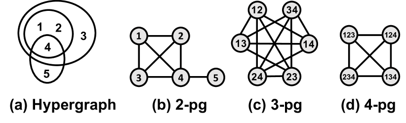
Figure 1. Hypergraph and its $n$-projected graphs ($n$-pgs). Edge weights, dropped for simplicity, reflect $n$-way interactions. For example, edge weight between the 3-pg nodes {1, 2} and {2, 3} is the number of times {1, 2, 3} interacted as a group.

That is, each node $v_{n}$ in the $n$-projected graph $G_{n}$ of a hypergraph $G$ is a size-($n$-$1$) subset of nodes in $G$, and each edge $(u_{n},v_{n})$ represents a size-$n$ subset of nodes in $G$ contained in at least one hyperedge in $G$. The weight of an edge corresponds to the sum of weights of hyperedges in $G$ that contain the size-$n$ subset represented by the edge. In other words, the weight of each edge indicates how often the corresponding $n$ nodes interact as a group and thus how close they are as a group. Notice that the pairwise projected graph is a special case of the $n$-projected graph where $n=2$. Figure 1 gives a visual description.

Based on $n$-projected graphs, we define the $n$-order expansion, our proposed way of incrementally approximating a hypergraph.

Definition 4.2 ($n$-order expansion).

The $\mathbf{n}$-order expansion $G^{(n)}$ of a hypergraph $G$ is a collection of $k$-projected graphs where $k$ varies from $2$ to $n$. That is, $G^{(n)}:=(G_{2},\ldots,G_{n}).$

As $n$ increases, the $n$-order representation $G^{(n)}$ captures more information in $G$, and if $n$ reaches its maximum, $G$ can be reconstructed from $G^{(n)}$. In Section 5, we experimentally study the value of marginal information gain (quantified by prediction accuracy) for each $n$ in the $n$-order expansion in hyperedge prediction.

4.2. Prediction model

In this subsection, we describe the features and classifier that we use for hyperedge prediction.

Features. The $n$-order expansion of a hypergraph $G$ returns a series of $n$-projected graphs, from each of which we extract one among six features. Let $N_{n}(v_{n})$ be the set of neighbors of the node $v_{n}$ in the $n$-projected graph $G_{n}$, and for each subset $c$ of nodes in $G$, let $E_{n}(c):=\{(u_{n},v_{n})\in E_{n}:u_{n}\subseteq c\text{ and }v_{n}\subseteq c\}$ be the set of “inner” edges in $G_{n}$ that represent a subset of $c$. Then, we use the following features extractable from $G_{n}$ for each hyperedge candidate $c\in C$:

$\circ$ Geometric mean (GM):	$x_{n}(c)=\Big{(}\prod_{e_{n}\in E_{n}(c)}\omega_{n}(e_{n})\Big{)}^{\frac{1}{|E_{n}(c)|}}$
$\circ$ Harmonic mean (HM):	$x_{n}(c)=\frac{|E_{n}(c)|}{\sum_{e_{n}\in E_{n}(c)}\omega_{n}(e_{n})^{-1}}$
$\circ$ Arithmetic mean (AM):	$x_{n}(c)=\frac{1}{|E_{n}(c)|}\sum_{e_{n}\in E_{n}(c)}\omega_{n}(e_{n})$
$\circ$ Common neighbors (CN):	$x_{n}(c)=\bigcap_{v_{n}\subseteq c}N_{n}(v_{n})$
$\circ$ Jaccard coefficient (JC):	$x_{n}(c)=\frac{\bigcap_{v_{n}\subseteq c}N_{n}(v_{n})}{\bigcup_{v_{n}\subseteq c}N_{n}(v_{n})}$
$\circ$ Adamic-Adar index (AA):	$x_{n}(c)=\sum\limits_{u_{n}\in\bigcap_{v_{n}\subseteq c}N_{n}(v_{n})}\frac{1}{\log|N_{n}(u_{n})|}$

The first three measures (GM, HM, and AM) are the geometric, harmonic, and arithmetic means of inner edge weights in the $n$-projected graphs. These features are reported to work well in the task of predicting triangles in $2$-projected graphs (Benson et al., 2018a). For the other three measures (CN, JC, and AA), we extend well-known pairwise link prediction features (Newman, 2001; Salton and McGill, 1983; Adamic and Adar, 2003) to larger groups of nodes.

When the input hypergraph is represented in the form of the $n$-order expansion $G^{(n)}$, the features obtained in different projected graphs are concatenated. That is, the features of a subset $c$ of nodes obtained from $G^{(n)}$ are $[x_{2}(c),\ldots,x_{n}(c)]$.

Classifier. We use the above features as the inputs to a logistic regression classifier with L2 regularization, which has been used widely for link and hyperedge prediction (Grover and Leskovec, 2016; Benson et al., 2018a; Liben-Nowell and Kleinberg, 2007). Although complicated classifiers with more parameters, such as deep neural networks, could be used instead, their performance has higher variance and depends more heavily on hyperparameter values. We decide to use the simple classifier to provide stable comparisons of different orders of approximation.

5. Experiments

In this section, we present our experimental results to address our questions on the impact of higher-order interactions in the form of $n$-projected graphs (or simply $n$-pgs throughout this section).

5.1. Setup

We start by explaining our datasets and the experimental setup, followed by our results in each of subsections.

Datasets. We use 15 datasets generated across 8 domains from (Benson et al., 2018a). The numbers of edges and hyperedges in them are summarized in Table 1. Hyperedges in each domain are defined as follows: (a) Email (email-Enron (Klimt and Yang, 2004), email-Eu (Yin et al., 2017)): recipient addresses of an email, (b) Contact (contact-primary-school (Stehlé et al., 2011), contact-high-school (Mastrandrea et al., 2015)): persons that appeared in face-to-face proximity, (c) Drug components (NDC-classes, NDC-substances): classes or substances within a single drug, listed in the National Drug Code Directory, (d) Drug use (DAWN): drugs used by a patient, reported to the Drug Abuse Warning Network, before an emergency visit, (e) US Congress (congress-bills (Fowler, 2006b)): congress members cosponsoring a bill, (f) Online tags (tags-ask-ubuntu, tags-math-sx): tags in a question in Stack Exchange forums, (g) Online threads (tags-ask-ubuntu, tags-math-sx): users answering a question in Stack Exchange forums, and (h) Coauthorship (coauth-MAG-History (Sinha et al., 2015), coauth-MAG-Geology (Sinha et al., 2015), coauth-DBLP): coauthors of a publication. We only consider hyperedges containing at most 10 nodes. It is reported that large hyperedges are rare and less meaningful (Benson et al., 2018a). As mentioned in Section 3.2, the datasets are timestamped but we treat them as weighted hypergraphs with unique hyperedges.

Training and evaluation. For each target hyperedge size (4, 5, 10), we generate positive hyperedges $C_{p}$ by randomly removing hyperedges until $60\%$ of all hyperedges or no hyperedges with the target size are left. We randomly sample the sets of nodes that form cliques and stars in 2-pg as negative hyperedges $C_{n}$ until a certain multiple of positive hyperedges ($\times$ 1, 2, 5, 10, 200) are gathered (see Section 3.3 for details). The positive and negative hyperedges are combined to form the candidate set, i.e., $C=C_{p}\sqcup C_{n}$. The candidate set $C$ is split into train $(50\%)$ and test $(50\%)$ sets. We evaluate classification performance by the area under the precision-recall curve (AUC-PR) (Davis and Goadrich, 2006), a measure sensitive to class imbalance.

Table 1. Dataset statistics. We count the number of unique hyperedges and the number of edges in the 2,3,4-projected graphs. More details are provided in (app, 2020).

Dataset	$|E|$	$|E_{2}|$	$|E_{3}|$	$|E_{4}|$
email-Enron	1,491	1,442	8,916	25,938
email-Eu	24,223	21,465	143,238	440,916
contact-primary-school	12,704	8,317	15,417	2,286
contact-high-school	7,818	5,818	7,110	1,428
NDC-classes	901	3,727	21,885	61,176
NDC-substances	8,167	26,973	234,240	729,012
DAWN	137,417	97,046	1,456,683	4,917,996
congress-bills	57,887	178,647	2,439,960	8,117,514
tags-ask-ubuntu	147,222	132,703	838,107	874,056
tags-math-sx	170,476	91,685	748,644	936,774
threads-ask-ubuntu	166,995	186,955	181,881	116,046
threads-math-sx	595,648	1,083,531	2,184,567	2,174,994
coauth-MAG-History	891,296	723,382	2,101,608	4,226,058
coauth-MAG-Geology	1,189,770	4,241,817	18,870,564	40,067,280
coauth-DBLP	2,454,734	7,123,888	26,398,201	46,071,251

Table 2. Performance gain of $n$ to $(n+1)$-order expansion. Gain is computed as percentage improvement in AUC-PR. For predicting size 4 hyperedges, we use 2 and 3-order expansions. For predicting size 5, we use 2, 3, and 4-order expansions. Increasing the order of expansion gives better performance (marked in bold) in most cases, across datasets and features. Results on every task variation are in (app, 2020).

	Size 4 prediction						Size 5 prediction
	2 to 3 gain (%)						2 to 3 gain (%)						3 to 4 gain (%)
Dataset	GM	HM	AM	CN	JC	AA	GM	HM	AM	CN	JC	AA	GM	HM	AM	CN	JC	AA
email-Enron	12.67	0.49	-0.15	33.89	-1.57	35.78	14.37	22.59	5.95	10.73	-2.98	17.01	-1.53	-0.59	-0.26	5.04	1.59	-2.05
email-Eu	0.69	-0.13	1.67	153.81	9.16	148.09	-2.44	-0.78	4.04	158.79	13.93	157.73	0.64	-0.32	1.23	2.01	18.86	2.31
contact-primary-school	6.42	1.21	49.2	495.94	413.35	484.73	0	0	6.63	708.56	361.79	267.66	0	0	0	0	0	0
contact-high-school	15.16	-0.87	78.62	515.17	455.54	507.13	0	0	14.14	1623.33	221.51	1617.75	0	5.96	3.9	0	104.37	0
NDC-classes	0.18	4.23	-44.70	1.55	10.91	2.25	44.28	16.62	-37.82	0.28	10.07	5.60	6.77	16.95	-2.31	-4.14	2.00	-1.50
NDC-substances	-4.95	-0.02	0.47	0.57	-40.98	-3.54	10.73	2.46	0.16	16.01	-17.02	14.18	158.10	0.02	7.07	-1.81	-0.47	-2.99
DAWN	0.15	0.04	21.34	197.97	30.48	187.62	0.23	3e-4	3.48	220.79	42.80	212.33	0.49	4e-4	14.04	-0.85	17.31	-0.54
congress-bills	7.92	-0.99	14.53	328.76	16.49	294.16	11.84	-0.03	30.86	271.64	48.55	259.22	-0.07	4.98	0.26	0.93	0.57	0.16
tags-ask-ubuntu	0.24	-0.51	23.09	216.47	14.07	192.03	0.07	0.02	20.84	244.72	80.37	225.89	1e-05	-1.13	2.96	0.85	5.50	1.35
tags-math-sx	0.46	0.18	32.38	137.4	46.53	127.25	0.13	0.01	21.35	146.02	60.64	135.54	1e-05	0.63	9.73	0.67	5.86	0.74
threads-ask-ubuntu	2e-3	10.05	2.47	2.34	2.34	1.48	-1e-3	-1.76	6.51	2.56	3.10	1.76	-1e-4	9.62	-0.07	0.01	-0.05	1e-3
threads-math-sx	0.03	0.44	8.52	6.01	5.61	5.10	5e-3	0.42	23.48	6.63	6.56	5.65	1e-3	0.61	0.01	2e-4	-0.15	-4e-6
coauth-MAG-History	4e-3	-8.48	-1.81	1.69	3.00	1.94	0.08	0.13	3.00	2.32	4.43	2.37	0.16	137.94	2.36	-0.23	0.53	-0.10
coauth-MAG-Geology	0.93	0.36	22.93	15.39	19.76	15.34	0.79	3.78	603.02	14.56	20.52	14.65	-30.08	0.17	8.14	-0.10	1.68	0.39
coauth-DBLP	-53.43	0.90	145.31	16.89	21.99	16.73	1.32	3.52	175.24	16.17	22.82	15.44	-24.05	0.58	11.06	-0.08	1.69	0.30
Average	-0.90	0.46	23.60	141.59	67.11	134.41	5.43	3.16	58.73	229.54	58.47	220.85	7.36	11.69	3.88	0.15	10.62	-0.13

5.2. Results and messages

In this subsection, we present our results by summarizing them with three main messages.

 

(M1) More higher-order information leads to better prediction quality, but with diminishing returns.

 

We investigate how the prediction performance changes with increasing $n$ in $n$-order expansions. In particular, we predict hyperedges of size 4 with the features from 2 and 3-order expansions, and hyperedges of size 5 with features from 2, 3, and 4-order expansions. Table 2 summarizes the results, and for readers’ convenience, we also plot the performance averaged across all features in Figure 2.

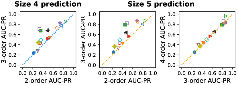
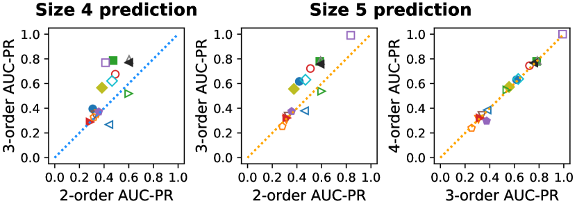
Figure 2. Performance comparison between order $n$ and $n+1$. Performance is averaged across features. Nodes that form cliques (upper) and stars (lower) in 2-pg are used as negative hyperedges. Class imbalance is set to 1:10. While there is overall performance gain, the gain from 3 to 4 is smaller than 2 to 3.

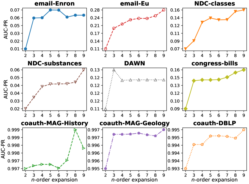
Figure 3. Diminishing returns of $n$-order expansions. We set target size as 10 and observe until 9-order expansions. We exclude datasets that has no edges in any of the projected graphs, and we set the class imbalance to 1:200. We take the average performance across all features except the geometric mean, whose value can become too large in higher-order pgs. As $n$ grows, performance tend to increase. However, gains tend to decrease.

We clearly observe that higher-order expansion gives better performance, where the improvement quantity differs across datasets and features. Performance gaps from $n=2$ to $n=3$, averaged across features, are 61% for size 4 and 94% for size 5, respectively, whereas it is just 6% for size 5 from $n=3$ to $n=4.$ As for the individual features, we see that the gain is larger with neighborhood-based features (CN, JC, AA) than with mean-based features (GM, HM, AM). The mean values are small in higher-order pgs, while neighborhood-based features still retain meaningfully large values. Entries with exactly zero gain (contact datasets) result from the sparsity of size 5 hyperedges (i.e., $<10$). See more details in (app, 2020).

Interestingly, we see the diminishing returns as $n$ increases. To study this, we predict size 10 hyperedges with $n$-order expansions for $n=2,3,\ldots,9.$ Figure 3 shows that, in most datasets, the performances tend to increase significantly from $n=2$ to $n=3$, but marginally for $n\geq 3$. However, somewhat unexpectedly, we also find that some datasets experience a small jump (not as high as that from $n=2$ to $n=3$) from $n=7$ to $n=8$ (NDC-classes, coauth-MAG-History) or from $n=8$ to $n=9$ (NDC-substances, coauth-MAG-Geology, coauth-DBLP). We speculate that it is because knowing 8 or 9-way interactions is often more useful compared to knowing those between 4 to 7-way, for predicting size 10. For illustration, papers with 10 authors would be often made by a group of 9 existing collaborators’ invitation of another author.

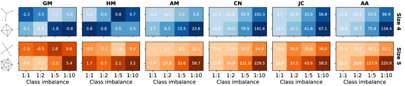
Figure 4. How task difficulty affects the utility of higher-order information. The value in each box is 2 to 3-order gain (%) averaged across datasets. Boxes with larger gain are colored with greater intensity. We see that as task gets harder, higher-order information helps more.

 

(M2) More hardness of the task gives higher values to higher-order information.

 

As discussed in Section  3.3, we adjust the hardness level in hyperedge prediction by varying the negative set $C_{n}$ in terms of negative hyperedge types (stars and cliques) and class imbalances (1:1, 1:2, 1:5, 1:10). We investigate the impact of those variations on the performance gain, summarized in Figure 4. The $y$ axis represents the types of negative hyperedges (stars or cliques), extracted from 2-pg, and the $x$ axis represents different class imbalances.

Regarding the types of negative hyperedges, we see that the gains from $n=2$ to $n=3$ are larger for cliques than stars. As explained in Section 3.3, distinguishing whether a clique is a true hyperedge or not is a much harder task compared to a star. The troubleshooter is 3-pg, that is, to refer to higher-order information. On the impact of class imbalance, again the gain from $n=2$ to $n=3$ is larger, as class imbalance grows. More negative hyperedges imply the increasing hardness in obtaining better precision, while maintaining the same sensitivity, and there are more negative hyperedges that resemble positive hyperedges. In such cases, incorporating 3-pg in addition to 2-pg, provided that it gives more information, helps distinguish fake samples better. Note that in GM, there are reversed tendencies. This is explained by the property of GM (i.e., geometric mean defined in Section 4.2) that a pairwise disconnection makes $x_{n}(c)=0$, i.e., strict stars are easily filtered with only 2-pg, since $x_{2}(c)=0$.

 

(M3) Higher-order information helps more, when (i) higher-order interactions are more frequent, and (ii) higher-order interactions share less information with pairwise ones.

 

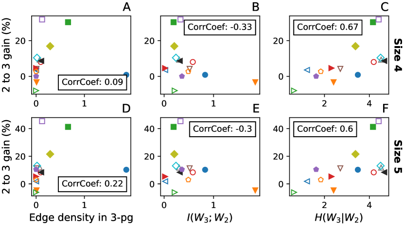
Figure 5. Interpreting the differences of higher-order gain across datasets. Edge density in 3-pg (A, D) and conditional entropy (C, F) has positive correlation with performance gain. Mutual information (B, E) has negative correlation. Plots are shown for cliques with class imbalance of 1:1. Results on all cases are in (app, 2020).

We observe different performance gains across different datasets in the two prior messages. For example, in Table 2, the average gain from $n=2$ to $n=3$ was about 284% in contact-primary-school, while it was merely 6.5% in NDC-classes. We now delve into why they do, for which we measure various statistics, including the edge density and information-theoretic values of some pgs.

(a) Edge density in 3-pg. We first examine edge density in 3-pg, i.e., $\frac{\text{\# edges in 3-pg}}{\text{\# all possible 3-way interactions}}\times 100\%$. This intuitively quantifies the abundance of 3-way interactions. We measure the Pearson correlation coefficient between edge density and performance gain, as shown in Figures 5-A and D. We observe positive correlations between those two, 0.22 and 0.09 for size 5 and size 4 predictions, respectively, implying that more frequent higher-order interactions let higher-order representation lead to better prediction.

(b) Mutual information and conditional entropy. We next study the aforementioned observation with information-theoretic measures. We expect that adding 3-pg would have larger returns when it contains more information exclusive to itself. We set two joint random variables $W_{2}$ and $W_{3}$ generated by three different nodes sampled $v_{1},v_{2},v_{3}\in V$ uniformly at random, representing a vector of the weights of three pairwise edges and the weight of a triadic edge, i.e., $W_{2}:=\big{(}\omega_{2}(v_{1},v_{2}),\omega_{2}(v_{2},v_{3}),\omega_{2}(v_{1},v_{3})\big{)},$ and $W_{3}:=\omega_{3}(v_{1},v_{2},v_{3}).$ We consider mutual information $I(W_{3};W_{2})$ and conditional entropy $H(W_{3}|W_{2})$. Note that $I(W_{3};W_{2})$ quantifies the amount of shared information between $W_{2}$ and $W_{3}$, while $H(W_{3}|W_{2})$ is the remaining information (i.e., uncertainty) of $W_{3}$ given information of $W_{2}$.

Figures 5-B and E show negative correlations -0.33 and -0.3 between the mutual information and performance gain, and similarly, Figures 5-C and F show positive correlations 0.67 and 0.6 between the conditional entropy and performance gain. These results imply that the gain from $n=2$ to $n=3$ is large when 3-pg is difficult to be explained in terms of 2-pg. We find that the conditional entropy has greater absolute correlations compared to the mutual information. A possible explanation is that the conditional entropy directly quantifies the information gain while the mutual information focuses on the shared information of 2-pg and 3-pg.

6. Discussion and conclusion

In this paper, we studied how much abstraction of group interactions is needed to accurately represent a hypergraph, with hyperedge prediction as our downstream task. We devise the $n$-projected graph to capture the $n$-way interactions in a hypergraph, and express the hypergraph with a collection of $n$-projected graphs. We investigate the performance gain as $n$ grows. We conclude that small $n$ is sufficient due to the diminishing returns, and higher $n$ acts as a troubleshooter in difficult task settings. We provide interpretations why different datasets have different gains. In summary, we investigate 1) how much, 2) when, and 3) why higher-order representations provide better accuracy. We expect that our results would offer insights to relevant works that follow. We leave our source code at (app, 2020).

- (1)
- app (2020) 2020. Supplementary Document. Available online: https://github.com/granelle/www20-higher-order. (2020).
- Adamic and Adar (2003) Lada A Adamic and Eytan Adar. 2003. Friends and neighbors on the web. Social networks 25, 3 (2003), 211–230.
- Agarwal et al. (2006) Sameer Agarwal, Kristin Branson, and Serge Belongie. 2006. Higher order learning with graphs. In ICML.
- Agarwal et al. (2005) Sameer Agarwal, Jongwoo Lim, Lihi Zelnik-Manor, Pietro Perona, David Kriegman, and Serge Belongie. 2005. Beyond pairwise clustering. In CVPR.
- Arya and Worring (2018) Devanshu Arya and Marcel Worring. 2018. Exploiting Relational Information in Social Networks using Geometric Deep Learning on Hypergraphs. In ACM Multimedia.
- Benson et al. (2018a) AR Benson, R Abebe, MT Schaub, A Jadbabaie, and J Kleinberg. 2018a. Simplicial closure and higher-order link prediction. Proceedings of the National Academy of Sciences of the United States of America 115, 48 (2018).
- Benson et al. (2018b) Austin R Benson, Ravi Kumar, and Andrew Tomkins. 2018b. Sequences of sets. In KDD.
- Bu et al. (2010) Jiajun Bu, Shulong Tan, Chun Chen, Can Wang, Hao Wu, Lijun Zhang, and Xiaofei He. 2010. Music recommendation by unified hypergraph: combining social media information and music content. In ACM Multimedia.
- Bulò and Pelillo (2009) Samuel R Bulò and Marcello Pelillo. 2009. A game-theoretic approach to hypergraph clustering. In NeurIPS.
- Chen et al. (2009) Gang Chen, Jianwen Zhang, Fei Wang, Changshui Zhang, and Yuli Gao. 2009. Efficient multi-label classification with hypergraph regularization. In CVPR.
- Davis and Goadrich (2006) Jesse Davis and Mark Goadrich. 2006. The relationship between Precision-Recall and ROC curves. In ICML.
- Fatemi et al. (2019) Bahare Fatemi, Perouz Taslakian, David Vazquez, and David Poole. 2019. Knowledge Hypergraphs: Extending Knowledge Graphs Beyond Binary Relations. arXiv:1906.00137 (2019).
- Feng et al. (2019) Yifan Feng, Haoxuan You, Zizhao Zhang, Rongrong Ji, and Yue Gao. 2019. Hypergraph neural networks. In AAAI.
- Fowler (2006a) James H. Fowler. 2006a. Connecting the Congress: A Study of Cosponsorship Networks. Political Analysis 14, 04 (2006), 456–487.
- Fowler (2006b) James H. Fowler. 2006b. Legislative cosponsorship networks in the US House and Senate. Social Networks 28, 4 (2006), 454–465.
- Ghoshdastidar and Dukkipati (2017) Debarghya Ghoshdastidar and Ambedkar Dukkipati. 2017. Uniform hypergraph partitioning: Provable tensor methods and sampling techniques. The Journal of Machine Learning Research 18, 1 (2017), 1638–1678.
- Grover and Leskovec (2016) Aditya Grover and Jure Leskovec. 2016. node2vec: Scalable feature learning for networks. In KDD.
- Grover et al. (2019) Aditya Grover, Aaron Zweig, and Stefano Ermon. 2019. Graphite: Iterative Generative Modeling of Graphs. In ICML.
- Hu et al. (2008) Tianming Hu, Hui Xiong, Wenjun Zhou, Sam Yuan Sung, and Hangzai Luo. 2008. Hypergraph partitioning for document clustering: A unified clique perspective. In SIGIR.
- Huang et al. (2015b) Jin Huang, Rui Zhang, and Jeffrey Xu Yu. 2015b. Scalable hypergraph learning and processing. In ICDM.
- Huang et al. (2015a) Sheng Huang, Mohamed Elhoseiny, Ahmed Elgammal, and Dan Yang. 2015a. Learning hypergraph-regularized attribute predictors. In CVPR.
- Hwang et al. (2008) TaeHyun Hwang, Ze Tian, Rui Kuangy, and Jean-Pierre Kocher. 2008. Learning on weighted hypergraphs to integrate protein interactions and gene expressions for cancer outcome prediction. In ICDM.
- Karypis et al. (1999) George Karypis, Rajat Aggarwal, Vipin Kumar, and Shashi Shekhar. 1999. Multilevel hypergraph partitioning: applications in VLSI domain. IEEE Transactions on Very Large Scale Integration Systems 7, 1 (1999), 69–79.
- Karypis and Kumar (2000) George Karypis and Vipin Kumar. 2000. Multilevel k-way hypergraph partitioning. VLSI design 11, 3 (2000), 285–300.
- Klamt et al. (2009) Steffen Klamt, Utz-Uwe Haus, and Fabian Theis. 2009. Hypergraphs and cellular networks. PLoS computational biology 5, 5 (2009), e1000385.
- Klimt and Yang (2004) Bryan Klimt and Yiming Yang. 2004. The enron corpus: A new dataset for email classification research. In ECML PKDD.
- Kolda and Bader (2009) Tamara G Kolda and Brett W Bader. 2009. Tensor decompositions and applications. SIAM review 51, 3 (2009), 455–500.
- Leskovec et al. (2007) Jure Leskovec, Jon Kleinberg, and Christos Faloutsos. 2007. Graph evolution: Densification and shrinking diameters. ACM Transactions on Knowledge Discovery from Data 1, 1 (2007).
- Li et al. (2013) Dong Li, Zhiming Xu, Sheng Li, and Xin Sun. 2013. Link prediction in social networks based on hypergraph. In WWW.
- Li et al. (2018) Jianbo Li, Jingrui He, and Yada Zhu. 2018. E-tail product return prediction via hypergraph-based local graph cut. In KDD.
- Liben-Nowell and Kleinberg (2007) David Liben-Nowell and Jon Kleinberg. 2007. The link prediction problem for social networks. Journal of the American society for information science and technology 58, 7 (2007), 1019–1031.
- Lin et al. (2009) Yu-Ru Lin, Jimeng Sun, Paul Castro, Ravi Konuru, Hari Sundaram, and Aisling Kelliher. 2009. Metafac: community discovery via relational hypergraph factorization. In KDD.
- Lü and Zhou (2011) Linyuan Lü and Tao Zhou. 2011. Link prediction in complex networks: A survey. Physica A: statistical mechanics and its applications 390, 6 (2011), 1150–1170.
- Mastrandrea et al. (2015) Rossana Mastrandrea, Julie Fournet, and Alain Barrat. 2015. Contact patterns in a high school: a comparison between data collected using wearable sensors, contact diaries and friendship surveys. PloS one 10, 9 (2015), e0136497.
- Navlakha and Kingsford (2010) Saket Navlakha and Carl Kingsford. 2010. The power of protein interaction networks for associating genes with diseases. Bioinformatics 26, 8 (2010), 1057–1063.
- Newman (2001) Mark EJ Newman. 2001. Clustering and preferential attachment in growing networks. Physical review E 64, 2 (2001), 025102.
- Ofli et al. (2017) Ferda Ofli, Yusuf Aytar, Ingmar Weber, Raggi Al Hammouri, and Antonio Torralba. 2017. Is saki# delicious?: The food perception gap on instagram and its relation to health. In WWW.
- Ouyang et al. (2002) Min Ouyang, Michel Toulouse, Krishnaiyan Thulasiraman, Fred Glover, and Jitender S Deogun. 2002. Multilevel cooperative search for the circuit/hypergraph partitioning problem. IEEE Transactions on Computer-Aided Design of Integrated Circuits and Systems 21, 6 (2002), 685–693.
- Salton and McGill (1983) Gerard Salton and Michael J McGill. 1983. Introduction to modern information retrieval. mcgraw-hill.
- Santolini and Barabási (2018) Marc Santolini and Albert-László Barabási. 2018. Predicting perturbation patterns from the topology of biological networks. Proceedings of the National Academy of Sciences 115, 27 (2018), E6375–E6383.
- Sharma et al. (2014) Ankit Sharma, Jaideep Srivastava, and Abhishek Chandra. 2014. Predicting multi-actor collaborations using hypergraphs. arXiv:1401.6404 (2014).
- Shashua et al. (2006) Amnon Shashua, Ron Zass, and Tamir Hazan. 2006. Multi-way clustering using super-symmetric non-negative tensor factorization. In ECCV.
- Sinha et al. (2015) Arnab Sinha, Zhihong Shen, Yang Song, Hao Ma, Darrin Eide, Bo-June (Paul) Hsu, and Kuansan Wang. 2015. An Overview of Microsoft Academic Service (MAS) and Applications. In WWW.
- Stehlé et al. (2011) Juliette Stehlé, Nicolas Voirin, Alain Barrat, Ciro Cattuto, Lorenzo Isella, Jean-François Pinton, Marco Quaggiotto, Wouter Van den Broeck, Corinne Régis, Bruno Lina, et al. 2011. High-resolution measurements of face-to-face contact patterns in a primary school. PloS one 6, 8 (2011), e23176.
- Tan et al. (2014) Shulong Tan, Ziyu Guan, Deng Cai, Xuzhen Qin, Jiajun Bu, and Chun Chen. 2014. Mapping users across networks by manifold alignment on hypergraph. In AAAI.
- Xu et al. (2013) Ye Xu, Dan Rockmore, and Adam M Kleinbaum. 2013. Hyperlink prediction in hypernetworks using latent social features. In DS.
- Yadati et al. (2018a) Naganand Yadati, Madhav Nimishakavi, Prateek Yadav, Anand Louis, and Partha Talukdar. 2018a. Hypergcn: Hypergraph convolutional networks for semi-supervised classification. arXiv:1809.02589 (2018).
- Yadati et al. (2018b) Naganand Yadati, Vikram Nitin, Madhav Nimishakavi, Prateek Yadav, Anand Louis, and Partha Talukdar. 2018b. Link Prediction in Hypergraphs using Graph Convolutional Networks. openreview.net (2018).
- Yang et al. (2019) Dingqi Yang, Bingqing Qu, Jie Yang, and Philippe Cudre-Mauroux. 2019. Revisiting user mobility and social relationships in lbsns: a hypergraph embedding approach. In WWW.
- Yin et al. (2017) Hao Yin, Austin R Benson, Jure Leskovec, and David F Gleich. 2017. Local higher-order graph clustering. In KDD.
- You et al. (2019) Jiaxuan You, Rex Ying, and Jure Leskovec. 2019. Position-aware Graph Neural Networks. In ICML.
- Zhang et al. (2018) Muhan Zhang, Zhicheng Cui, Shali Jiang, and Yixin Chen. 2018. Beyond link prediction: Predicting hyperlinks in adjacency space. In AAAI.
- Zhang (2019) Yang Zhang. 2019. Language in Our Time: An Empirical Analysis of Hashtags. In WWW.
- Zhou et al. (2017) Chang Zhou, Yuqiong Liu, Xiaofei Liu, Zhongyi Liu, and Jun Gao. 2017. Scalable graph embedding for asymmetric proximity. In AAAI.
- Zhou et al. (2007) Dengyong Zhou, Jiayuan Huang, and Bernhard Schölkopf. 2007. Learning with hypergraphs: Clustering, classification, and embedding. In NeurIPS.
- Zhu et al. (2016) Yu Zhu, Ziyu Guan, Shulong Tan, Haifeng Liu, Deng Cai, and Xiaofei He. 2016. Heterogeneous hypergraph embedding for document recommendation. Neurocomputing 216 (2016), 150–162.