Multiple Object Tracking by Flowing and Fusing

Abstract

Most of Multiple Object Tracking (MOT) approaches compute individual target features for two subtasks: estimating target-wise motions and conducting pair-wise Re-Identification (Re-ID). Because of the indefinite number of targets among video frames, both subtasks are very difficult to scale up efficiently in end-to-end Deep Neural Networks (DNNs). In this paper, we design an end-to-end DNN tracking approach, Flow-Fuse-Tracker (FFT), that addresses the above issues with two efficient techniques: target flowing and target fusing. Specifically, in target flowing, a FlowTracker DNN module learns the indefinite number of target-wise motions jointly from pixel-level optical flows. In target fusing, a FuseTracker DNN module refines and fuses targets proposed by FlowTracker and frame-wise object detection, instead of trusting either of the two inaccurate sources of target proposal. Because FlowTracker can explore complex target-wise motion patterns and FuseTracker can refine and fuse targets from FlowTracker and detectors, our approach can achieve the state-of-the-art results on several MOT benchmarks. As an online MOT approach, FFT produced the top MOTA of 46.3 on the 2DMOT15, 56.5 on the MOT16, and 56.5 on the MOT17 tracking benchmarks, surpassing all the online and offline methods in existing publications. 

1 Introduction

Multiple Object Tracking (MOT) [69, 42] is a critical perception technique required in many computer vision applications, such as autonomous driving [8], field robotic [50] and video surveillance [71]. One of the most popular MOT settings is tracking-by-detection [70], in which the image-based object detection results are available in each frame, and MOT algorithms basically associate the same target between frames. Because of occlusion, diversity of motion patterns and the lack of tracking training data, MOT under the tracking-by-detection setting remains a very challenging task in computer vision.

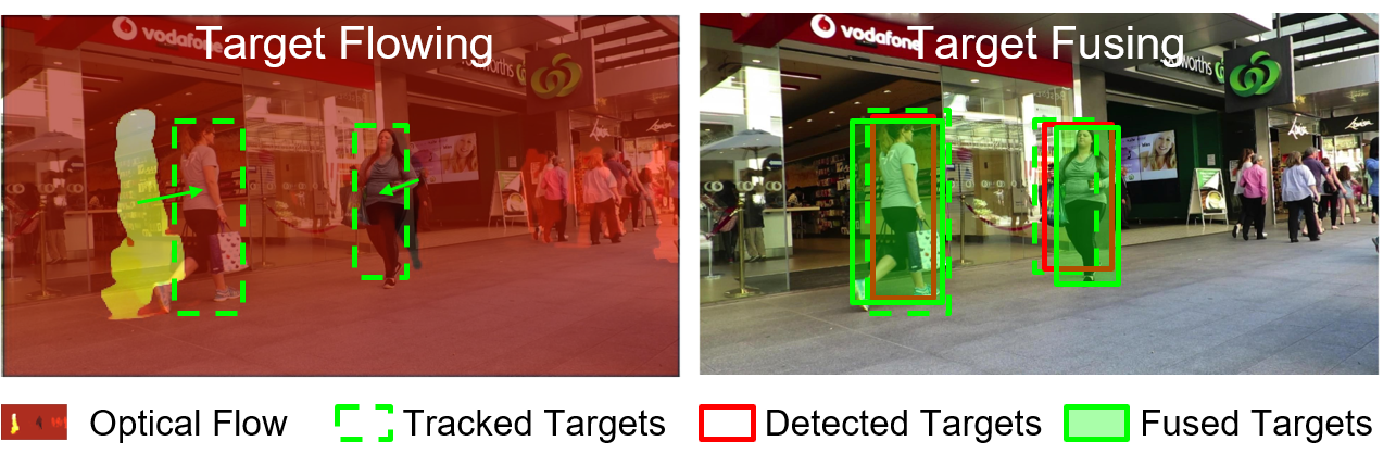
Figure 1: Multiple object tracking by target flowing and target fusing. Target Flowing: a FlowTracker DNN module learns indefinite number of target-wise motion jointly from frame-wise optical flows. Target Fusing: a FuseTracker DNN module jointly refines and fuses targets from FlowTracker and image based object detection, instead of trusting either of the two inaccurate sources of target proposal. (Best viewed in color)

Recent MOT approaches [25, 3] use Deep Neural Networks (DNNs) to model individual target motions and compare pairwise appearances for target association. Benefiting from the powerful representation capability of DNNs, both the target-wise features for motion and pair-wise features for appearance have been significantly improved to boost the MOT performance. However, the computation of both features is very difficult to scale up efficiently for indefinite number of targets among video frames. For instance, to compare pair-wise appearances among indefinite number of targets, one needs to process indefinite number of pairs iteratively using fixed-structured DNNs.

In practice, most approaches solve the MOT problem in two separated steps: 1) Run a motion model and an appearance model on input frames to produce motion and appearance features, respectively; and 2) Conduct target association between frames based on the motion and appearance features. In general, the target association step finds one-to-one matches using the Hungarian algorithm [32]. However, because the two steps are not optimized in an end-to-end framework, a heavy DNN is usually needed to learn highly discriminative motion and appearance features. Without nearly perfect features, numerous candidate target pairs and heuristic tricks need to be processed in the target association step. Therefore, it is very hard to develop an efficient MOT system when the feature extraction and data association are treated as two separate modules.

In this paper, we design an end-to-end DNN tracking approach, Flow-Fuse-Tracker (FFT), that addresses the above issues with two efficient techniques: target flowing and target fusing. The end-to-end nature of FFT significantly boosts the MOT performance even without using the time-consuming pairwise appearance comparison. As shown in Figure 1, FFT applies target flowing, a FlowTracker DNN module, to extract multiple target-wise motions from pixel-level optical flows. While in target fusing, a FuseTracker DNN module refines and fuses targets proposed by FlowTracker and frame-wise object detection, instead of trusting either of the two inaccurate sources of target proposal. In the training process, we simply take two regression losses and one classification loss to update the weights of both FlowTracker and FuseTracker DNN modules. As a result, the FlowTracker learns complex target-wise motion patterns from simple pixel-level motion clues, and the FuseTracker gains the ability to further refine and fuse inaccurate targets from FlowTracker and object detectors. Given paired frames as input, FFT will directly output the target association results in the tracking process.

In summary, the main contributions of our work can be highlighted as follows:

• An end-to-end DNN tracking approach, called FFT, that jointly learns both target motions and associations for MOT.

• A FlowTracker DNN module that jointly learns indefinite number of target-wise motions from pixel-level optical flows.

• A FuseTracker DNN module that directly associates the indefinite number of targets from both tracking and detection.

• As an online MOT method, FFT achieves the state-of-the-art results among all the existing online and offline approaches.

2 Related Work

Because most of the existing MOT methods consist of a motion model and an appearance model, we review variants of each model, respectively.

Motion Models. The motion models try to describe how each target moves from frame to frame, which is the key to choose an optimal search region for each target in the next frame. The existing motion models can be roughly divided into two categories, i,e., single-target models and multi-target models. In particular, the single-object models usually apply the linear methods [28, 43, 45, 72] or nonlinear methods [15, 67] to estimate the motion pattern of each object across adjacent frames. In the earlier works, the Kalman filter [28] has been widely used to estimate motions in many MOT methods [1, 2, 61]. In recent years, a large number of deep learning based methods are designed to model motion patterns given sequences of target-wise locations. For example, the Long Short Term Memory (LSTM) networks [42, 52, 31] describe and predict complex motion patterns of each target over multiple frames. Different from single-target approaches, the multi-target models aim to estimate the motion patterns of all the targets in each frame, simultaneously. Representative methods take optical flows [65, 22, 30], LiDAR point clouds [62, 29], or stereo point clouds [44, 4] as inputs to estimate different motion patterns. All these approaches use frame-wise point/pixel-level motion as a feature to match individual objects. Their matching processes are clustering in nature, which leverages multiple features such as trajectory and appearances. In comparison, our FlowTracker is a simple regression module that directly estimates target-wise motion from the category-agnostic optical flow.

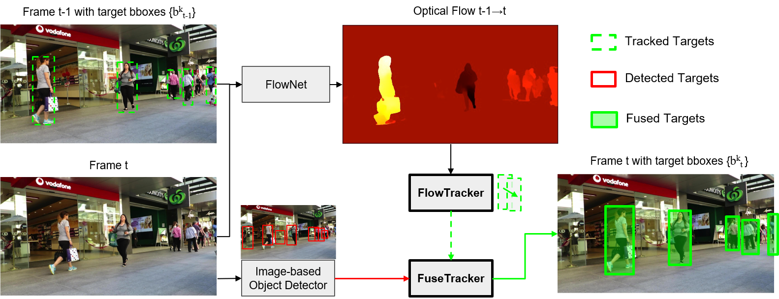
Figure 2: The overall view of Flow-Fuse-Tracker (FFT) for multiple object tracking. FlowTracker and FuseTracker (in bold grey boxes) are the two DNN modules of our FFT network. In the FlowTracker, the optical flow is generated from two sequential frames, and the target bboxes $\{b^{k}_{t-1}\}$ (green dashed bboxes) at frame $t-1$ are regressed to the bboxes $\{b^{k}_{t}\}$ at frame $t$ through the optical flow. In the FuseTracker, the bboxes from both $\{b^{k}_{t}\}$ and public detections $D_{t}$ (red bboxes) at frame $t$ are refined and fused. The FuseTracker outputs the final tracking results (green bboxes with shadow). (Best viewed in color)

Appearance Model. The appearance models aim to learn discriminative features of targets, such that features of the same targets across frames are more similar than those of different targets. In the earlier tracking approaches, the color histogram [12, 36, 33] and pixel-based template representations [64, 46] are standard hand-crafted features used to describe the appearance of moving objects. In addition to using Euclidean distances to measure appearance similarities, the covariance matrix representation is also applied to compare the pixel-wise similarities, such as the SIFT-like features [23, 38] and pose features [51, 47]. In recent years, the deep feature learning based methods have been popularized with the blooming of DNNs. For example, the features of multiple convolution layers are explored to enhance the discriminative capability of resulting features [10]. In [3], an online feature learning model is designed to associate both the detection results and short tracklets. Moreover, different network structures, such as siamese network [34], triplet network [49] and quadruplet network [56], have been extensively used to learn the discriminative features cropped from the detected object bounding boxes. Benefiting from the powerful representation capability of DNNs, this line of methods [59, 57, 21] have achieved very promising results on the public benchmark datasets. However, most of these approaches extract discriminative features independently for each object bounding box, which is very costly when scaling-up to indefinite number of objects in MOT settings.

3 Our Method

To achieve an end-to-end MOT DNN, the fundamental demands are to jointly process the indefinite number of targets in both motion estimation and target association.

We address these demands with two techniques: 1) Target Flowing. Instead of extracting the target-wise features from images, our FlowTracker first estimates the motions of all pixels by optical flow and then refines the motion for each target. This technique shares the pixel-level appearance matching of optical flow over all targets. 2) Target Fusing. Instead of comparing features between targets, our FuseTracker fuses targets by refining their bounding boxes and merging the refined targets. These operations are conducted by a single DNN module, FuseTracker, such that targets from different sources (tracking and detection) can be associated based on the refined bounding boxes and confidence scores. Similar to the post-processing of standard object detectors, FuseTracker uses the efficient non-max-suppression (NMS) algorithm to produce the fused the targets.

Figure 2 shows the FFT architecture that enclose FlowTracker and FuseTracker. The details of FlowTracker and FuseTracker are introduced below.

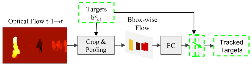
Figure 3: Network architecture of our FlowTracker.

3.1 FlowTracker Module

The FlowTracker DNN module aims to estimate indefinite number of target-wise motion jointly from pixel-level features, i.e., optical flow. The network architecture of our FlowTracker is shown in Figure 3, in which we just take several convolutional layers and one fully-connected (FC) layer to estimate the target motion from the previous frame to the current frame. Once our FlowTracker is trained, it just takes two frames as input and outputs multiple target motions between the two input frames.

The previous frame is denoted as $\mathbf{I}_{t-1}\in\mathbb{R}^{3\times w\times h}$, and the current frame is represented by $\mathbf{I}_{t}\in\mathbb{R}^{3\times w\times h}$, where $t>1$ indicates the time index. Firstly, we feed the two frames into the FlowNet, and a pixel-wise optical flow $\mathbf{F}_{t}\in\mathbb{R}^{2\times w\times h}$ can be obtained at the output layer. Secondly, we take the resulting optical flow into our FlowTracker, and train it using the ground truth motion vectors. In practice, the previous frame usually has multiple targets to be tracked in the current frame. For simplicity, we denote targets in the previous frame as $\mathbf{B}_{t-1}=\{\mathbf{b}_{t-1}^{k1},\mathbf{b}_{t-1}^{k2},\ldots,\mathbf{b}_{t-1}^{kn}|1\leq k_{1},k_{2},\ldots,k_{n}\leq N\}$, where $\mathbf{b}_{t-1}^{k}=(x_{t-1}^{k},y_{t-1}^{k},w_{t-1}^{k},h_{t-1}^{k})$ indicates the position of $k\in\{k_{1},k_{2},\ldots,k_{n}\}$ target in frame $\mathbf{I}_{t-1}$. The corresponding targets in the current frame are denoted by $\mathbf{B}_{t}=\{\mathbf{b}_{t}^{k1},\mathbf{b}_{t}^{k2},\ldots,\mathbf{b}_{t}^{kn}|1\leq k_{1},k_{2},\ldots,k_{n}\leq N\}$, where $\mathbf{b}_{t}^{k}=(x_{t}^{k},y_{t}^{k},w_{t}^{k},h_{t}^{k})$ indicates the position of $k\in\{k_{1},k_{2},\ldots,k_{n}\}$ target in frame $\mathbf{I}_{t}$. As a result, the target motions can be easily learned by measuring the difference between $\mathbf{B}_{t-1}$ and $\mathbf{B}_{t}$. The loss function for target motion is:

$$L_{1}(\Delta\mathbf{B}_{t},\Delta\mathbf{B}_{t}^{*})=\|\Delta\mathbf{B}_{t}-\Delta\mathbf{B}_{t}^{*}\|_{F}^{2}.$$ (1)

where $\Delta\mathbf{B}_{t}^{*}=\mathbf{B}_{t}-\mathbf{B}_{t-1}$ indicates the ground truth motion vectors of all targets between frame $\mathbf{I}_{t-1}$ and $\mathbf{I}_{t}$, and $\Delta\mathbf{B}_{t}$ denotes the output motion vectors by our FlowTracker DNN module. By optimizing this objective function to update the parameters of FlowTracker DNN module in the training process, our FlowTracker gains ability to predict the target motions $\Delta\mathbf{B}_{t}=\{[\Delta x_{t}^{k},\Delta y_{t}^{k},\Delta w_{t}^{k},\Delta h_{t}^{k}]\}$ from frame $\mathbf{I}_{t-1}$ to $\mathbf{I}_{t}$. As a result, we can easily estimate the target positions in the current frame as $\mathbf{B}_{t}=\mathbf{B}_{t-1}+\Delta\mathbf{B}_{t}$. When more and more target motions are consistently learned in the training process, our FlowTracker become stronger to associate targets across the adjacent frames.

3.2 FuseTracker Module

The FuseTracker DNN module aims to jointly refine and fuse targets tracked from FlowTracker $\mathbf{B}_{t}=\{b_{t}^{k_{1}},b_{t}^{k_{2}},\ldots,b_{t}^{k_{n}}|1\leq k_{1},k_{2},\ldots,k_{n}\leq N\}$ and the target detections $\mathbf{D}_{t}=\{d_{t}^{i}\}|_{i=1,\ldots,m}$ from image-based object detectors. The network architecture of FuseTracker is shown in Figure 4. Our FuseTracker is modified from the well-known Faster-RCNN [48]. Specifically, we add the Feature Pyramid Networks (FPN) [37] to extract features from different scales. In testing, we remove the Region Proposal Network (RPN), and use the FlowTracker targets and public detection bboxes as proposals.

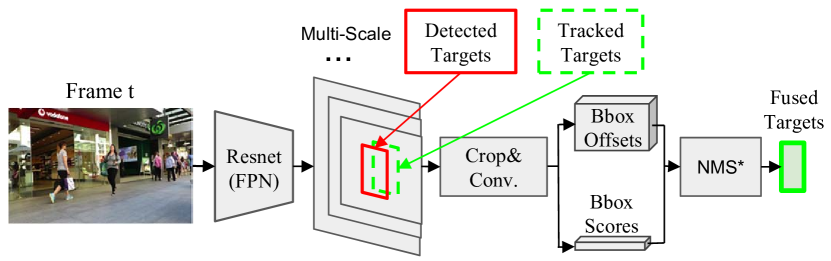
Figure 4: Network architecture of our FuseTracker.

Neither the targets from FlowTracker nor the objects from image-based detector can be directly used as targets passing along to the next frames. On one hand, targets from our FlowTracker contains identity (ID) index $\{k_{1},k_{2},\ldots,k_{n}|1\leq k_{1},k_{2},\ldots,k_{n}\leq N\}$ inherited from the $\bf{I}_{t-1}$, but may have inaccurate bboxes in frame $t$. On the other hand, the objects from image-based detector require ID assignment, either taking the IDs of FlowTracker targets or generating new IDs. Moreover, even if some FlowTracker targets and detected objects can be matched, it is still unclear which bboxes should be used for targets in frame $t$.

FuseTracker resolves this issue by treating both FlowTracker targets $\mathbf{B}_{t}$ and detected objects $\mathbf{D}_{t}$ equally as proposals. Formally, FuseTracker takes bbox proposals from both $\mathbf{B}_{t}$ and $\mathbf{D}_{t}$, and current frame $\mathbf{I}_{t}$ as input. For each proposal, FuseTracker estimates its offset $\Delta(cx,cy,w,h)$ and confidence score $c$. Given the two refined bbox sets $\mathbf{B}_{t}^{ref}$ and $\mathbf{D}_{t}^{ref}$, FuseTracker firstly deals with disappeared objects by killing the bboxes with low confidence scores. Then two-level NMS (shown as “NMS*” in Figure 4) are applied to merge the bboxes. In particular, the first level NMS is applied within the refined FlowTracker targets and detected objects to handle the object mutual occlusion. The second level NMS is conducted with Intersection over Union (IoU) based bbox matching and max-score selection. This level of NMS assigns IDs from FlowTracker targets to detected objects, and produces more accurate bboxes for the fused targets. All the detected objects that do not inherit target IDs are treated as new targets.

In training FuseTracker, similar to Faster-RCNN [48], the RPN generates multiple scales of bounding box proposals, and the feature maps are cropped by each proposal. Then the Region of Interest (RoI) pooling is applied to the cropped feature maps, which are later passed to both bbox classification head and regression head to get object classification score and bbox location offsets, respectively. Given the predicted classification score, location offset and ground truth bounding boxes, we minimize an objective function following the multi-task loss [24]. The loss function for the detection head is defined as:

$$L_{2}(c,c^{*},b,b^{*})=L_{cls}(c,c^{*})+\lambda[c^{*}\geq 1]L_{reg}(b,b^{*}),$$ (2)

where $c$ and $b=(x,y,w,h)$ are the predicted classification score and bounding box location, respectively. $c^{*}$ and $b^{*}$ are the corresponding ground truth. The classification loss $L_{cls}$ is log loss and the regression loss $L_{reg}$ is the smooth L1 loss. Particularly, the weights for the RPN part are fixed during training since we just want to use the RPN to produce bbox proposals which imitates the FlowTracker output and public detection results.

In the testing stage of FuseTracker, we remove the RPN, and use the FlowTracker targets $\mathbf{B}_{t}$ and bounding boxes from public detectors $\mathbf{D}_{t}$ as proposals.

3.3 Inference algorithm

The FFT inference algorithm runs the FlowTracker and FuseTracker jointly to produce MOT outputs (see details in Algorithm 1). In summary, there are $7$ steps in the FFT inference algorithm:

• Step 1. The detections in the first frame $\mathbf{D}_{0}$ is refined by the FuseTracker. The detected bboxes are passed to FuseTracker as the proposals. Among the output bboxes of FuseTracker, those whose confidence scores are smaller than $\mathrm{thresh\_score}$ are killed and frame-wised NMS is applied. The refined detection $\mathbf{D}_{0}^{ref}$ is used to initialize the trajectory set $\mathbf{T}$. (Line 2-7)

• Step 2. The detections for the current frame $\mathbf{D}_{t}$ is refined by the FuseTracker in the same way as Step 1. (Line 8)

• Step 3. All the tracked bboxes $\mathbf{B}_{t-1}$ (bboxes with trajectory IDs) in previous frame $\mathbf{I}_{t-1}$ are found in $\mathbf{T}$. The FlowTracker takes the image pair $\{\mathbf{I}_{t-1},\mathbf{I}_{t}\}$ and $\mathbf{B}_{t-1}$ as input, and produces the corresponding tracked bboxes $\mathbf{B}_{t}$ in the current frame $\mathbf{I}_{t}$. (Line 9-11)

• Step 4. The FuseTracker fuses the bboxes from $\mathbf{B}_{t}$ and $\mathbf{D}_{t}^{ref}$. We first refine the $\mathbf{B}_{t}$ the same way as described in Step 1. Then, for each tracked bbox $\mathbf{b}_{t}^{k}$ in $\mathbf{B}_{t}^{ref}$, we find the bbox that has the largest IoU from $\mathbf{D}_{t}^{ref}$. If this IoU is larger than $\mathrm{thresh\_iou}$, we consider this detected bbox is matched to $\mathbf{b}_{t}^{k}$. If the confidence score for the matched detected bbox is higher than $\mathbf{b}_{t}^{k}$’s score, we use the detected bbox to replace $\mathbf{b}_{t}^{k}$. Besides, the NMS is applied to the fused bbox set to get the tracked bbox result $\mathbf{B}_{t}^{trk}$. The FuseTracker returns the NMS output $\mathbf{B}_{t}^{trk}$ and the unmatched detections $\mathbf{D}_{t}^{umt}$. (Line 12)

• Step 5. The bboxes in $\mathbf{B}_{t}^{trk}$ are add to the corresponding trajectories in $\mathbf{T}$. (Line 13)

• Step 6. For the unmatched detections $\mathbf{D}_{t}^{umt}$, we conduct backtracking (see more details below) to match them with trajectories $\mathbf{T}_{nas}$ (trajectories not successfully associated in the current frame by Step 2-5). (Line 14-19)

• Step 7. The detections that cannot be matched by backtracking $\mathbf{D}_{t}^{umt^{\prime}}$ are initialized as new trajectories. (Line 20)

Backtracking. In the tracking process, some targets are occluded or out-of-scene in the previous frames and re-emerge in the current frame. To handle these cases, one needs to track repeatedly between the current frame and several previous frames. We call this process BackTracking (BT). To be specific, for the trajectories $\mathbf{T}_{nas}$, we try to find bboxes of these trajectories $\mathbf{B}_{nas}$ for the earlier frames. We apply the FlowTracker to shift bboxes in $\mathbf{B}_{nas}$ from previous frames to $\mathbf{B}_{t}^{\prime}$ in the current frame. Then the FuseTracker is applied to fuse the unmatched detections $\mathbf{D}_{t}^{umt}$ and $\mathbf{B}_{t}^{\prime}$. Here, we only consider the trajectories that could be matched with the detections. Finally, we add the tracked bboxes $\mathbf{B}_{t}^{trk^{\prime}}$ to the corresponding trajectories. The more previous frames used in BT, the more likely all targets can be tracked despite of occlusions. We study the effects of the number of BT frames in the ablation studies section below. However, the inference overheads increase with the increase of BT frames. For efficient implementation, we apply different numbers of BTs adaptively at different frames and process multiple BTs in one batch.

Algorithm 1 Flow-Fuse-Tracker

1:Video sequence $\mathbf{I}=\{\mathbf{I}_{t}\}_{t=0}^{T-1}$ of frame $\mathbf{I}_{t}$ at time $t$; Public detection set $\mathbf{D}=\{\mathbf{D}_{t}\}_{t=0}^{T-1}$ of detections $\mathbf{D}_{t}$ for frame $\mathbf{I}_{t}$

2:Trajectory set $\mathbf{T}=\{\mathbf{T}^{k}\}_{k=1}^{M}$, where $\mathbf{T}^{k}=\{\mathbf{b}_{t}^{k}\}_{t=0}^{T-1}$ with $\mathbf{b}_{t}^{k}=(x,y,w,h,t)$

3:$\mathbf{T}\leftarrow\O$

4:for $\mathbf{I}_{t},\mathbf{D}_{t}$ $in$ $\mathrm{zip}(\mathbf{I},\mathbf{D})$ do

5:     if $t==0$ then

6:         $\mathbf{D}_{0}^{ref}\leftarrow\mathrm{FuseTracker}(\mathbf{I}_{0},\mathbf{D}_{0})$

7:         Initialize the trajectory set $\mathbf{T}$ with $\mathbf{D}_{0}^{ref}$

8:         continue

9:     end if

10:     $\mathbf{D}_{t}^{ref}\leftarrow\mathrm{FuseTracker}(\mathbf{I}_{t},\mathbf{D}_{t})$

11:     $\mathbf{B}_{t-1}\leftarrow$ find all tracked $\mathbf{b}_{t-1}^{k}$ at $\mathbf{I}_{t}$ from $\mathbf{T}$

12:     $\mathbf{I}_{pair}\leftarrow\{\mathbf{I}_{t-1},\mathbf{I}_{t}\}$

13:     $\mathbf{B}_{t}\leftarrow\mathrm{FlowTracker}(\mathbf{I}_{pair},\mathbf{B}_{t-1})$

14:     $\mathbf{B}_{t}^{trk},\mathbf{D}_{t}^{umt}\leftarrow\mathrm{FuseTracker}(\mathbf{B}_{t},\mathbf{D}_{t}^{ref})$

15:     $\mathbf{T}\leftarrow$ update $\mathbf{B}_{t}^{trk}$ to the corresponding $\mathbf{T}^{k}$

16:     $\mathbf{T}_{nas}\leftarrow$ find tracks $\mathbf{T}^{k}$ that do not have $\mathbf{b}_{t}^{k}$

17:     $\mathbf{I}_{pairs}{}\leftarrow$ get image pairs for back tracking, $\mathbf{I}_{pairs}=\{\{\mathbf{I}_{t},\mathbf{I}_{t-2}\},\{\mathbf{I}_{t},\mathbf{I}_{t-3}\},\ldots,\{\mathbf{I}_{t},\mathbf{I}_{t-\mathrm{BT}}\}\}$

18:     $\mathbf{B}_{nas}\leftarrow$ get tracked bboxes from $\mathbf{T}_{nas}$ for back tracking, $\mathbf{B}_{nas}=\{\mathbf{B}_{t-2},\mathbf{B}_{t-3},\ldots,\mathbf{B}_{t-\mathrm{BT}}\}$

19:     $\mathbf{B}_{t}^{{}^{\prime}}\leftarrow\mathrm{FlowTracker}(\mathbf{I}_{pairs},\mathbf{B}_{nas})$

20:     $\mathbf{B}_{t}^{trk^{\prime}},\mathbf{D}_{t}^{umt^{\prime}}\leftarrow\mathrm{FuseTracker}(\mathbf{B}_{t}^{{}^{\prime}},\mathbf{D}_{t}^{umt})$

21:     $\mathbf{T}\leftarrow$ update $\mathbf{B}_{t}^{trk^{\prime}}$ to the corresponding $\mathbf{T}^{k}$

22:     $\mathbf{T}\leftarrow$ initialize new trajectories with $\mathbf{D}_{t}^{umt^{\prime}}$

23:end for

24:return $\mathbf{T}$

4 Experiments

FFT is implemented in Python with PyTorch framework. Extensive experiments have been conducted on the MOT benchmarks, including the 2DMOT2015 [35], MOT16 [41], and MOT17 [41]. In particular, we compare FFT with the latest published MOT approaches, perform ablation studies on the effectiveness of FuseTracker, FlowTracker and BackTracking frames, and also analyze the influence of target sizes and percentages of occlusion on the performance of FFT.

Method	MOTA $\uparrow$	MOTP $\uparrow$	IDF1 $\uparrow$	IDP $\uparrow$	IDR $\uparrow$	MT $\uparrow$	ML$\downarrow$	FP $\downarrow$	FN $\downarrow$	ID Sw. $\downarrow$	Frag. $\downarrow$
FFT w/o FuseTracker	50.1	75.7	44.2	58.5	35.6	18.8%	33.1%	27,213	248,011	6,429	6,956
FFT w/o FlowTracker	55.8	77.5	49.3	60.8	41.5	26.1%	27.1%	31,172	210,196	7,866	5,519
FFT	56.5	77.8	51.0	64.1	42.3	26.2%	26.7%	23,746	215,971	5,672	5,474

Table 1: Ablation study of FFT on the effectiveness of FuseTracker and FlowTracker on the MOT17 benchmark. (Best in bold)

Ablation	MOTA $\uparrow$	MOTP $\uparrow$	IDF1 $\uparrow$	IDP $\uparrow$	IDR $\uparrow$	MT $\uparrow$	ML$\downarrow$	FP $\downarrow$	FN $\downarrow$	ID Sw. $\downarrow$	Frag. $\downarrow$
FFT-BT1	55.9	77.8	40.2	50.6	33.4	26.3%	26.7%	23,540	215,740	9,789	5,495
FFT-BT10	56.4	77.8	49.1	61.8	40.7	26.2%	26.7%	23,683	215,941	6,227	5,479
FFT-BT20	56.5	77.8	50.3	63.3	41.7	26.2%	26.7%	23,743	216,000	5,810	5,484
FFT-BT30	56.5	77.8	51.0	64.1	42.3	26.2%	26.7%	23,746	215,971	5,672	5,474

Table 2: Ablation study of FFT on the number of Backtracking frames (BT#) on the MOT17 benchmark. (Best in bold)

4.1 Experiment Setting

Training. FlowTracker consists of a FlowNet2 [27] component and a regression component. The FlowNet2 is pre-trained on MPI-Sintel [7] dataset and its weights are fixed during the training of the regression component. In the training process of our FlowTracker, we use the Adam optimizer and set the initial learning rate to 1e-4, divided by 2 at the epoch 80, 160, 210 and 260, respectively. We train the model for 300 epochs with a batch size of 24.

FuseTracker is modified from the Faster-RCNN, in which we take ResNet101+FPN as the backbone. The backbone network is initialized with the ImageNet pre-trained weights and the whole model is trained with the ground truth bounding boxes from the MOT datasets. In the training process of our FuseTracker, we use the Stochastic Gradient Descent (SGD) optimizer and set the initial learning rate to 1e-4, divided by 10 every 5 epochs. We train the model for 20 epochs with a batch size of 16.

Inference. As described in 3.3, the FFT inference algorithm is specified by three parameters: the confidence score threshold $\mathrm{thresh\_score}$, the IoU threshold $\mathrm{thres\_iou}$, the NMS threshold $\mathrm{thresh\_nms}$, and the number of backtracking frames. In particular, we use $\mathrm{thresh\_score}$ = 0.5, $\mathrm{thresh\_iou}$ = 0.5 and $\mathrm{thresh\_nms}$ = 0.5 for all the benchmark datasets in our experiment. We use different backtracking frames for different datasets due to their frame rate difference. The settings are specified in 4.2. Also the effects of BT frames were studied in 4.3.

4.2 Main Results

Datasets. We use three benchmark datasets, including the 2DMOT2015 [35], MOT16 [41], and MOT17 [41], to conduct our experiments. All of them contain video sequences captured by both static and moving cameras in unconstrained environments, e.g., under the complex scenes of illumination changes, varying viewpoints and weather conditions. The 2DMOT2015 benchmark contains 22 video sequences, among which 11 videos sequences are for testing. The 2DMOT2015 benchmark provides ACF [16] detection results. The Frames Per Second (FPS) for each video in 2DMOT2015 varies from 2.5 to 30. Therefore we set our BT frames according to the FPS. We used BT frames 3 for low-FPS videos of 2.5, BT frames 10 for medium-FPS videos of 7 and 10, and BT frames 30 for high-FPS videos of 14, 25, and 30. The MOT16 benchmark includes $7$ fully annotated training videos and $7$ testing videos. The public detection results are obtained by DPM [19]. We use BT frames 30 for all the testing videos. The MOT17 benchmark is consist of $7$ fully annotated training videos and $7$ testing videos, in which public detection results are obtained by three image-based object detectors: DPM [19], FRCNN [48] and SDP [17]. The BT frames for all the testing videos are set to be 30.

Augmentation. We apply two types of augmentation methods for training the FlowTracker. In order to deal with the different movement speeds of multiple target objects and the different BT frames, we use different sampling rates to get the image pairs. Particularly, each video sequence is processed by 8 different sampling rates, which results in 8 sets. The intervals between the image frame numbers in each image pair for the 8 sets are 1, 3, 5, 10, 15, 20, 25, 30, respectively. Moreover, when we want to get target motion out of the pixel-wise optical flow, if the bbox location in the current frame is not accurate, the cropped flow feature will be incomplete but we still want to regress to the accurate bbox location in the next frame. Therefore, as shown in Figure 5, we apply jittering to the bboxes for regression. We enlarge or reduce the bbox height and width by a random ratio between 0 and 0.15. Also, we shift the center of the bbox vertically and horizontally by a random ratio between -0.15 and 0.15 of the width and height, respectively. We ensure the IoU between the original bbox and the bbox after jittering is larger than 0.8.

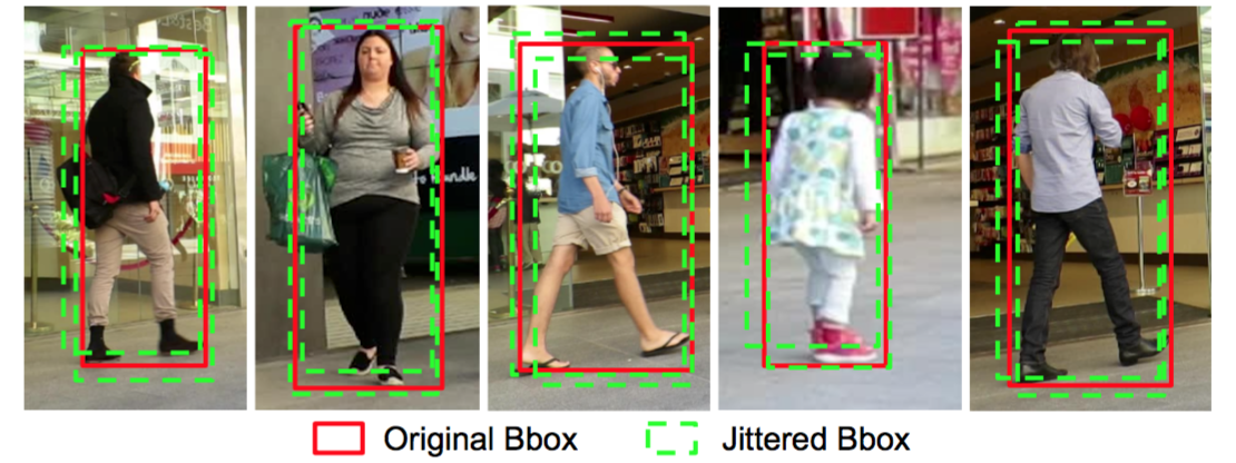
Figure 5: The jittering of the bounding boxes. The red bboxes are the ground truth bboxes. We apply the random jittering to them to slightly shift their positions and change their shapes, and we use the jittered bboxes (green dashed bboxes) in training the FlowTracker.

To train the FuseTracker, we just use horizontal flip as the augmentation.

	Method	MOTA $\uparrow$	MOTP $\uparrow$	IDF1 $\uparrow$	IDP $\uparrow$	IDR $\uparrow$	MT $\uparrow$	ML $\downarrow$	FP $\downarrow$	FN $\downarrow$	ID Sw. $\downarrow$	Frag. $\downarrow$
Offline	JointMC [30]	35.6	71.9	45.1	54.4	38.5	23.2%	39.3%	10,580	28,508	457	969
Online	INARLA [63]	34.7	70.7	42.1	51.7	35.4	12.5%	30.0%	9,855	29,158	1,112	2,848
	HybridDAT [68]	35.0	72.6	47.7	61.7	38.9	11.4%	42.2%	8,455	31,140	358	1,267
	RAR15pub [18]	35.1	70.9	45.4	62.0	35.8	13.0%	42.3%	6,771	32,717	381	1,523
	AMIR15 [52]	37.6	71.7	46.0	58.4	38.0	15.8%	26.8%	7,933	29,397	1,026	2,024
	STRN [66]	38.1	72.1	46.6	63.9	36.7	11.5%	33.4%	5,451	31,571	1,033	2,665
	AP_HWDPL_p [10]	38.5	72.6	47.1	68.4	35.9	8.7%	37.4%	4,005	33,203	586	1,263
	KCF [13]	38.9	70.6	44.5	57.1	36.5	16.6%	31.5%	7,321	29,501	720	1,440
	Tracktor [5]	44.1	75.0	46.7	58.1	39.1	18.0%	26.2%	6,477	26,577	1,318	1,790
	FFT(Ours)	46.3	75.5	48.8	54.8	44.0	29.1%	23.2%	9,870	21,913	1,232	1,638

Table 3: Comparison between FFT and other modern MOT methods on the 2DMOT15 benchmark. (Best in bold)

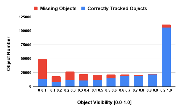
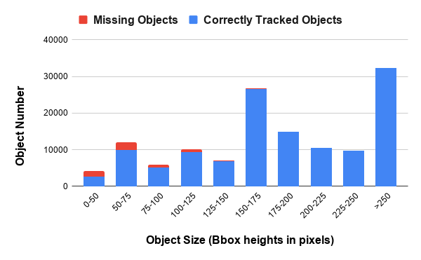
Figure 6: Effects of object visibility and object sizes on FFT (MOT17 training set).

Results. To evaluate the performance of our proposed method, we follow the CLEAR MOT Metrics [6]. We report the Multiple Object Tracking Precision (MOTP) and the Multiple Object Tracking Accuracy (MOTA) that combines three sources of errors: False Positives (FP), False Negatives (FN) and the IDentity Switches (IDS). Additionally, we also report the ID F1 Score (IDF1), ID Precision (IDP), ID Recall (IDR), the number of track fragmentations (Frag.), the percentage of mostly tracked targets (MT) and the percentage of mostly lost targets (ML). Among them, the MOTA score is the main criterium .

We compare FFT method with the latest MOT approaches we can find based on their published papers. Table 3, 4 and 5 list the MOT results of two main categories: offline trackers and online trackers. Note that offline trackers typically use information from both previous and future frames in tracking targets in the current frame, whereas online trackers only use knowledge from previous frames. Therefore, in terms of the main MOT metric, MOTA, offline trackers generally perform better than the online ones. However, FFT, which is an online method, outperforms all the MOT approaches in 2DMOT15, MOT16 and MOT17 benchmark in terms of MOTA as shown in Table 3, 4 and 5. Moreover, FFT also achieves the best performance in the mostly tracked targets (MT), the mostly lost targets (ML) and false negative (FN) metrics. It indicates that FFT could correctly track the most positions.

	Method	MOTA $\uparrow$	MOTP $\uparrow$	IDF1 $\uparrow$	IDP $\uparrow$	IDR $\uparrow$	MT $\uparrow$	ML $\downarrow$	FP $\downarrow$	FN $\downarrow$	ID Sw. $\downarrow$	Frag. $\downarrow$
Offline	FWT [26]	47.8	75.5	44.3	60.3	35.0	19.1%	38.2%	8,886	85,487	852	1,534
	GCRA [39]	48.2	77.5	48.6	69.1	37.4	12.9%	41.1%	5,104	88,586	821	1,117
	TLMHT [54]	48.7	76.4	55.3	76.8	43.2	15.7%	44.5%	6,632	86,504	413	642
	LMP [58]	48.8	79.0	51.3	71.1	40.1	18.2%	40.1%	6,654	86,245	481	595
	AFN [53]	49.0	78.0	48.2	64.3	38.6	19.1%	35.7%	9,508	82,506	899	1,383
	eTC [60]	49.2	75.5	56.1	75.9	44.5	17.3%	40.3%	8,400	83,702	606	882
	HCC [40]	49.3	79.0	50.7	71.1	39.4	17.8%	39.9%	5,333	86,795	391	535
	NOTA [9]	49.8	74.5	55.3	75.3	43.7	17.9%	37.7%	7,248	83,614	614	1,372
Online	MOTDT [11]	47.6	74.8	50.9	69.2	40.3	15.2%	38.3%	9,253	85,431	792	1,858
	STRN [66]	48.5	73.7	53.9	72.8	42.8	17.0%	34.9%	9,038	84,178	747	2,919
	KCF [13]	48.8	75.7	47.2	65.9	36.7	15.8%	38.1%	5,875	86,567	906	1,116
	LSSTO [20]	49.2	74.0	56.5	77.5	44.5	13.4%	41.4%	7,187	84,875	606	2,497
	Tracktor [5]	54.4	78.2	52.5	71.3	41.6	19.0%	36.9%	3,280	79,149	682	1,480
	FFT(Ours)	56.5	78.1	50.1	64.4	41.1	23.6%	29.4%	5,831	71,825	1,635	1,607

Table 4: Comparison between FFT and other modern MOT methods on the MOT16 benchmark. (Best in bold)

	Method	MOTA $\uparrow$	MOTP $\uparrow$	IDF1 $\uparrow$	IDP $\uparrow$	IDR $\uparrow$	MT $\uparrow$	ML $\downarrow$	FP $\downarrow$	FN $\downarrow$	ID Sw. $\downarrow$	Frag. $\downarrow$
Offline	jCC [30]	51.2	75.9	54.5	72.2	43.8	20.9%	37.0%	25,937	247,822	1,802	2,984
	NOTA [9]	51.3	76.7	54.5	73.5	43.2	17.1%	35.4%	20,148	252,531	2,285	5,798
	FWT [26]	51.3	77.0	47.6	63.2	38.1	21.4%	35.2%	24,101	247,921	2,648	4,279
	AFN17 [53]	51.5	77.6	46.9	62.6	37.5	20.6%	35.5%	22,391	248,420	2,593	4,308
	eHAF [55]	51.8	77.0	54.7	70.2	44.8	23.4%	37.9%	33,212	236,772	1,834	2,739
	eTC [60]	51.9	76.3	58.1	73.7	48.0	23.1%	35.5%	36,164	232,783	2,288	3,071
	JBNOT [26]	52.6	77.1	50.8	64.8	41.7	19.7%	35.8%	31,572	232,659	3,050	3,792
	LSST [20]	54.7	75.9	62.3	79.7	51.1	20.4%	40.1%	26,091	228,434	1,243	3,726
Online	MOTDT [11]	50.9	76.6	52.7	70.4	42.1	17.5%	35.7%	24,069	250,768	2,474	5,317
	STRN [66]	50.9	75.6	56.0	74.4	44.9	18.9%	33.8%	25,295	249,365	2,397	9,363
	FAMNet [14]	52.0	76.5	48.7	66.7	38.4	19.1%	33.4%	14,138	253,616	3,072	5,318
	LSSTO [20]	52.7	76.2	57.9	76.3	46.6	17.9%	36.6%	22,512	241,936	2,167	7,443
	Tracktor [5]	53.5	78.0	52.3	71.1	41.4	19.5%	36.6%	12,201	248,047	2,072	4,611
	FFT(Ours)	56.5	77.8	51.0	64.1	42.3	26.2%	26.7%	23,746	215,971	5,672	5,474

Table 5: Comparison between FFT and other modern MOT methods on the MOT17 benchmark. (Best in bold)

4.3 Ablation Study

This section presents the ablation study on the MOT17 benchmark. We show the effectiveness of our FuseTracker and FlowTracker in Table 1. We first remove the FuseTracker to prove it is effective. However, we do not have any cues to generate scores for bboxes without using FuseTracker. In order to keep the completeness of our algorithm logic, we retrain a small RPN-like network with ResNet18 backbone to produce the scores for bboxes. Besides, we choose to trust public detections more here since we do not have the refinement module anymore. FFT w/o FuseTracker in Table 1 shows that the MOTA improves by $6.4$ and the IDF1 improves by $6.8$ with FuseTracker. All the other metrics are also improved by including FuseTracker in FFT. Then, we show the FlowTracker is effective. By removing the FlowTracker, we directly use the bboxes in the previous frame as the tracked target proposals for the FuseTracker in the current frame. FFT w/o FlowTracker in Table 1 shows that with FlowTracker the MOTA improves by $0.7$ and the IDF1 improves by $1.7$. Almost all the other metrics are also improved by including FlowTracker in FFT.

We also study the effectiveness of BackTracking (BT). As shown in Table 2, BT highly affects the two main metrics MOTA and IDF1. We run FFT with fixed BT frame number of $1$, $10$, $20$, and $30$. As the BT frame number increases, the MOTA increases by $0.6$ to $56.5$ and the IDF1 increase by $10.8$ to $51.0$. The performance saturates at around BT30. The results show that with a bigger number of BT frames, FFT observes longer temporal clips and is more likely to track the occluded, out-of-scene and noisy objects.

4.4 Analysis

Finally we analyze the specific performance of FFT in more details. Since our FlowTracker computes pixel motion (optical flows) at the frame bases, its performance is likely to be affected by occlusion and object sizes. When an object is occluded in the current frame, optical flow may not match all pixels between frames. Moreover, computation of optical flow at the frame level seeks to average errors over all pixels, so the optical flow of small objects (fewer pixels) is more likely to be inaccurate, which will further affect the target-wise motion estimation. We show the effects of object visibility and object sizes in following experiments.

Since the ground truth of the MOT test sets is not publicly available, we perform our analysis on the MOT17 training set. Figure 6 reports the total number of correctly tracked objects and missing objects summed over three public object detectors of MOT17, with respect to the objects’ visibility and size respectively. Object visibility of a target bbox is computed as the ratio between non-overlapped area divided by its bbox area. As shown in the subfigure Object Visibility, at low visibility, more objects are missing. The percentage of correctly tracked objects rises as the visibility increases. After the object visibility reaches $0.8$, the correctly tracked object ratio becomes steady.

For the object size analysis, we only collect the objects whose visibility is higher than $0.8$ in order to reduce the variables in experiments. The size of an object is measured by its bbox height. In the subfigure Object Size, the percentage of correctly tracked objects rises as the object size increase. For the object size (bbox height) reaches $150$, the tracking performance is nearly perfect.

5 Conclusion

Flow-Fuse-Tracker (FFT) achieves new state-of-the-arts of MOT by addressing two fundamental issues in existing approaches: 1) how to share motion computation over indefinite number of targets. 2) how to fuse the tracked targets and detected objects. Our approach presents an end-to-end DNN solution to both issues and avoid pair-wise appearance-based Re-ID, which has been the costly and indispensable components of most existing MOT approaches. FFT is a very general MOT framework. The presented version can be further improved by using better optical flow networks in FlowTracker and more recent object detector structures in FuseTracker.

References

- [1] Anton Andriyenko and Konrad Schindler. Multi-target tracking by continuous energy minimization. In CVPR, 2011.
- [2] Anton Andriyenko, Konrad Schindler, and Stefan Roth. Discrete-continuous optimization for multi-target tracking. In CVPR, 2012.
- [3] Seung-Hwan Bae and Kuk-Jin Yoon. Confidence-based data association and discriminative deep appearance learning for robust online multi-object tracking. TPAMI, 2018.
- [4] Max Bajracharya, Baback Moghaddam, Andrew Howard, Shane Brennan, and Larry H Matthies. A fast stereo-based system for detecting and tracking pedestrians from a moving vehicle. The International Journal of Robotics Research, 2009.
- [5] Philipp Bergmann, Tim Meinhardt, and Laura Leal-Taixe. Tracking without bells and whistles. In ICCV, October 2019.
- [6] Keni Bernardin and Rainer Stiefelhagen. Evaluating multiple object tracking performance: The clear mot metrics. EURASIP Journal on Image and Video Processing, 2008(1):246309, May 2008.
- [7] D. J. Butler, J. Wulff, G. B. Stanley, and M. J. Black. A naturalistic open source movie for optical flow evaluation. In ECCV, 2012.
- [8] Chenyi Chen, Ari Seff, Alain Kornhauser, and Jianxiong Xiao. Deepdriving: Learning affordance for direct perception in autonomous driving. In ICCV, 2015.
- [9] Long Chen, Haizhou Ai, Rui Chen, and Zijie Zhuang. Aggregate tracklet appearance features for multi-object tracking. IEEE Signal Processing Letters, 2019.
- [10] Long Chen, Haizhou Ai, Chong Shang, Zijie Zhuang, and Bo Bai. Online multi-object tracking with convolutional neural networks. In ICIP, 2017.
- [11] Long Chen, Haizhou Ai, Zijie Zhuang, and Chong Shang. Real-time multiple people tracking with deeply learned candidate selection and person re-identification. In ICME, 2018.
- [12] Wongun Choi and Silvio Savarese. Multiple target tracking in world coordinate with single, minimally calibrated camera. In ECCV, 2010.
- [13] Peng Chu, Heng Fan, Chiu C Tan, and Haibin Ling. Online multi-object tracking with instance-aware tracker and dynamic model refreshment. In WACV. IEEE, 2019.
- [14] Peng Chu and Haibin Ling. Famnet: Joint learning of feature, affinity and multi-dimensional assignment for online multiple object tracking. In ICCV, October 2019.
- [15] Caglayan Dicle, Octavia I Camps, and Mario Sznaier. The way they move: Tracking multiple targets with similar appearance. In ICCV, 2013.
- [16] Piotr Dollar, Ron Appel, Serge Belongie, and Pietro Perona. Fast feature pyramids for object detection. IEEE Trans. Pattern Anal. Mach. Intell., 36(8):1532–1545, Aug. 2014.
- [17] Andreas Ess, Bastian Leibe, and Luc Van Gool. Depth and appearance for mobile scene analysis. In ICCV, 2007.
- [18] Kuan Fang, Yu Xiang, Xiaocheng Li, and Silvio Savarese. Recurrent autoregressive networks for online multi-object tracking. In WACV. IEEE, 2018.
- [19] Pedro F Felzenszwalb, Ross B Girshick, David McAllester, and Deva Ramanan. Object detection with discriminatively trained part-based models. TPAMI, 2010.
- [20] Weitao Feng, Zhihao Hu, Wei Wu, Junjie Yan, and Wanli Ouyang. Multi-object tracking with multiple cues and switcher-aware classification. arXiv preprint arXiv:1901.06129, 2019.
- [21] Tharindu Fernando, Simon Denman, Sridha Sridharan, and Clinton Fookes. Tracking by prediction: A deep generative model for mutli-person localisation and tracking. WACV, 2018.
- [22] Katerina Fragkiadaki, Weiyu Zhang, Geng Zhang, and Jianbo Shi. Two-granularity tracking: Mediating trajectory and detection graphs for tracking under occlusions. In ECCV, 2012.
- [23] Brian Fulkerson, Andrea Vedaldi, and Stefano Soatto. Localizing objects with smart dictionaries. In ECCV, 2008.
- [24] Ross Girshick. Fast r-cnn. In ICCV, Washington, DC, USA, 2015. IEEE Computer Society.
- [25] Roberto Henschel, Laura Leal-Taixe, Daniel Cremers, and Bodo Rosenhahn. Fusion of head and full-body detectors for multi-object tracking. In CVPR Workshops, 2018.
- [26] Roberto Henschel, Yunzhe Zou, and Bodo Rosenhahn. Multiple people tracking using body and joint detections. In CVPR Workshops, 2019.
- [27] E. Ilg, N. Mayer, T. Saikia, M. Keuper, A. Dosovitskiy, and T. Brox. Flownet 2.0: Evolution of optical flow estimation with deep networks. In CVPR, 2017.
- [28] Rudolph Emil Kalman. A new approach to linear filtering and prediction problems. Journal of Basic Engineering, 1960.
- [29] Achim Kampker, Mohsen Sefati, Arya S Abdul Rachman, Kai Kreisköther, and Pascual Campoy. Towards multi-object detection and tracking in urban scenario under uncertainties. In VEHITS, 2018.
- [30] Margret Keuper, Siyu Tang, Bjorn Andres, Thomas Brox, and Bernt Schiele. Motion segmentation & multiple object tracking by correlation co-clustering. TPAMI, 2018.
- [31] Chanho Kim, Fuxin Li, and James M Rehg. Multi-object tracking with neural gating using bilinear lstm. In ECCV, 2018.
- [32] Harold W Kuhn. The hungarian method for the assignment problem. Naval research logistics quarterly, 2(1-2):83–97, 1955.
- [33] Nam Le, Alexander Heili, and Jean-Marc Odobez. Long-term time-sensitive costs for crf-based tracking by detection. In ECCV, 2016.
- [34] Laura Leal-Taixé, Cristian Canton-Ferrer, and Konrad Schindler. Learning by tracking: Siamese cnn for robust target association. In CVPR Workshops, 2016.
- [35] L. Leal-Taixé, A. Milan, I. Reid, S. Roth, and K. Schindler. MOTChallenge 2015: Towards a benchmark for multi-target tracking. arXiv:1504.01942 [cs], Apr. 2015. arXiv: 1504.01942.
- [36] Bastian Leibe, Konrad Schindler, Nico Cornelis, and Luc Van Gool. Coupled object detection and tracking from static cameras and moving vehicles. TPAMI, 2008.
- [37] Tsung-Yi Lin, Piotr Dollár, Ross B. Girshick, Kaiming He, Bharath Hariharan, and Serge J. Belongie. Feature pyramid networks for object detection. In CVPR, 2017.
- [38] David G Lowe. Distinctive image features from scale-invariant keypoints. IJCV, 2004.
- [39] Cong Ma, Changshui Yang, Fan Yang, Yueqing Zhuang, Ziwei Zhang, Huizhu Jia, and Xiaodong Xie. Trajectory factory: Tracklet cleaving and re-connection by deep siamese bi-gru for multiple object tracking. In ICME, 2018.
- [40] Liqian Ma, Siyu Tang, Michael J Black, and Luc Van Gool. Customized multi-person tracker. In ACCV, 2018.
- [41] A. Milan, L. Leal-Taixé, I. Reid, S. Roth, and K. Schindler. MOT16: A benchmark for multi-object tracking. arXiv:1603.00831 [cs], Mar. 2016. arXiv: 1603.00831.
- [42] Anton Milan, S Hamid Rezatofighi, Anthony Dick, Ian Reid, and Konrad Schindler. Online multi-target tracking using recurrent neural networks. In AAAI, 2017.
- [43] Anton Milan, Konrad Schindler, and Stefan Roth. Multi-target tracking by discrete-continuous energy minimization. TPAMI, 2016.
- [44] Dennis Mitzel and Bastian Leibe. Taking mobile multi-object tracking to the next level: People, unknown objects, and carried items. In ECCV, 2012.
- [45] Shaul Oron, Aharon Bar-Hille, and Shai Avidan. Extended lucas-kanade tracking. In ECCV, 2014.
- [46] Stefano Pellegrini, Andreas Ess, Konrad Schindler, and Luc Van Gool. You’ll never walk alone: Modeling social behavior for multi-target tracking. In ICCV, 2009.
- [47] Zhen Qin and Christian R Shelton. Social grouping for multi-target tracking and head pose estimation in video. TPAMI, 2016.
- [48] Shaoqing Ren, Kaiming He, Ross Girshick, and Jian Sun. Faster r-cnn: Towards real-time object detection with region proposal networks. In NIPS, 2015.
- [49] Ergys Ristani and Carlo Tomasi. Features for multi-target multi-camera tracking and re-identification. In CVPR, 2018.
- [50] Patrick Ross, Andrew English, David Ball, Ben Upcroft, and Peter Corke. Online novelty-based visual obstacle detection for field robotics. In ICRA, 2015.
- [51] Markus Roth, Martin Bäuml, Ram Nevatia, and Rainer Stiefelhagen. Robust multi-pose face tracking by multi-stage tracklet association. In ICPR, 2012.
- [52] Amir Sadeghian, Alexandre Alahi, and Silvio Savarese. Tracking the untrackable: Learning to track multiple cues with long-term dependencies. In ICCV, 2017.
- [53] Han Shen, Lichao Huang, Chang Huang, and Wei Xu. Tracklet association tracker: An end-to-end learning-based association approach for multi-object tracking. arXiv preprint arXiv:1808.01562, 2018.
- [54] Hao Sheng, Jiahui Chen, Yang Zhang, Wei Ke, Zhang Xiong, and Jingyi Yu. Iterative multiple hypothesis tracking with tracklet-level association. TCSVT, 2018.
- [55] Hao Sheng, Yang Zhang, Jiahui Chen, Zhang Xiong, and Jun Zhang. Heterogeneous association graph fusion for target association in multiple object tracking. TCSVT, 2018.
- [56] Jeany Son, Mooyeol Baek, Minsu Cho, and Bohyung Han. Multi-object tracking with quadruplet convolutional neural networks. In CVPR, 2017.
- [57] Shijie Sun, Naveed Akhtar, HuanSheng Song, Ajmal Mian, and Mubarak Shah. Deep affinity network for multiple object tracking. TPAMI, 2018.
- [58] Siyu Tang, Mykhaylo Andriluka, Bjoern Andres, and Bernt Schiele. Multiple people tracking by lifted multicut and person re-identification. In CVPR, 2017.
- [59] Xingyu Wan, Jinjun Wang, Zhifeng Kong, Qing Zhao, and Shunming Deng. Multi-object tracking using online metric learning with long short-term memory. In ICIP, 2018.
- [60] Gaoang Wang, Yizhou Wang, Haotian Zhang, Renshu Gu, and Jenq-Neng Hwang. Exploit the connectivity: Multi-object tracking with trackletnet. In ACM Multimedia, 2018.
- [61] Nicolai Wojke, Alex Bewley, and Dietrich Paulus. Simple online and realtime tracking with a deep association metric. In ICIP, 2017.
- [62] Bichen Wu, Alvin Wan, Xiangyu Yue, and Kurt Keutzer. Squeezeseg: Convolutional neural nets with recurrent crf for real-time road-object segmentation from 3d lidar point cloud. In ICRA, 2018.
- [63] Hefeng Wu, Yafei Hu, Keze Wang, Hanhui Li, Lin Nie, and Hui Cheng. Instance-aware representation learning and association for online multi-person tracking. PR, 2019.
- [64] Zheng Wu, Ashwin Thangali, Stan Sclaroff, and Margrit Betke. Coupling detection and data association for multiple object tracking. In CVPR, 2012.
- [65] Christopher Xie, Yu Xiang, Zaid Harchaoui, and Dieter Fox. Object discovery in videos as foreground motion clustering. In CVPR, 2019.
- [66] Jiarui Xu, Yue Cao, Zheng Zhang, and Han Hu. Spatial-temporal relation networks for multi-object tracking. In ICCV, October 2019.
- [67] Bo Yang and Ram Nevatia. An online learned crf model for multi-target tracking. In CVPR, 2012.
- [68] Min Yang, Yuwei Wu, and Yunde Jia. A hybrid data association framework for robust online multi-object tracking. TIP, 2017.
- [69] Young-chul Yoon, Abhijeet Boragule, Young-min Song, Kwangjin Yoon, and Moongu Jeon. Online multi-object tracking with historical appearance matching and scene adaptive detection filtering. In AVSS, 2018.
- [70] Shun Zhang, Jinjun Wang, Zelun Wang, Yihong Gong, and Yuehu Liu. Multi-target tracking by learning local-to-global trajectory models. PR, 2015.
- [71] Sanping Zhou, Jinjun Wang, Jiayun Wang, Yihong Gong, and Nanning Zheng. Point to set similarity based deep feature learning for person re-identification. In CVPR, 2017.
- [72] Ji Zhu, Hua Yang, Nian Liu, Minyoung Kim, Wenjun Zhang, and Ming-Hsuan Yang. Online multi-object tracking with dual matching attention networks. In ECCV, 2018.