Supportive interactions in the noisy voter model

Abstract

Latane social impact theory predicts recruitment and supportive interactions being responsible for opinion formation. So far only recruitment interactions were considered in the voter models. Here we consider a noisy voter model with supportive interactions, which make voters less likely to change their opinions. This is similar to the voter models with freezing, but instead of interacting with their past selves voters get the support from their peers. We examine two different ways in which the support could be implemented: support deterring imitation as well as independence, support deterring imitation only. Both assumptions introduce strong drift into the model, which almost always overcomes the diffusion caused by the imitative behavior. The first assumption introduces strong attraction to a full consensus state, unless the support becomes too strong. The latter assumption promotes partial consensus, with surviving minority group.

1 Introduction

It is widely accepted that humans tend to become more alike as they intermingle. Yet somehow human societies remains heterogeneous: holding a variety of different beliefs, customs and opinions [1, 2]. Sometimes heterogeneity of the commonly held beliefs appears to be contradicting even scientific consensus on relatively simple matters [3, 4, 5, 6, 7]. Phenomenology and mechanisms of individual and collective opinion adoption have been investigated both from the socio–psychological point of view [8, 9, 10, 11] as well as by developing social models similar to the ones found in physics [12, 13, 14, 15, 16, 17, 18]. Most models considered in sociophysics involve binary opinions [12, 13, 14, 15, 16, 17, 18], though some multi–state generalizations of the binary models are also considered (see [19, 20, 21] for some recent examples). Prevalence of binary opinion models can be likely attributed to the heritage of the Ising model. Furthermore assuming binary opinions is often sufficient to reproduce major social phenomena. In contrast, computational social science seems to prefer models with continuous opinions, such as bounded confidence models [2].

Voter model is one of the most studied agent–based models in sociophysics [12, 13, 15, 14, 16, 17, 18]. While the original voter model [22] assumed competition between species, this simple imitation model has found its applications in opinion dynamics [23]. Original voter model has numerous generalizations, which explore the impact of variety of social interaction mechanisms. Some of the more well known generalizations include independent (or noisy) behavior [24], inflexibility [25, 26], anti–conformity [27, 28, 29], variety of interaction (network) topologies [30, 31], non–linear interactions [32, 33] and even memory [34, 35, 36, 37]. Voter model has also found applications outside the field of opinion dynamics, e.g., it was used as a base for the models of the financial markets [38, 39, 40, 41, 42].

Here we consider the effect of the supportive interactions on the noisy voter model. The noisy voter model is particularly interesting model as it involves two main social responses (as per the diamond model [8]) to the peer pressure: independence (referred to as variability in the diamond model) and conformity. The diamond model also predicts two additional social responses: anti–conformity and disregard (referred to as independence in the diamond model). Disregarding the peer pressure evidently does not change the system state, thus this mechanism would have no observable effect. Anti–conformity, on the other hand, would change the system state, but it can be easily shown that it is already included in the noisy voter model. Introducing anti–conformity simply readjusts model parameter values unless some additional assumptions are made, such as considering conformists and anti–conformists being two different agent types as in [27, 29], or assuming network topology with at least two cliques as in [28]. It is worth to note that these social responses have profound impact in other generalizations of the voter model, such as $q$-voter model [43].

Another well–known psychological theory is Latane social impact theory [9]. While this theory is mostly concerned with the magnitude of impact social forces have on the individuals, this theory unlike the diamond model [8] acknowledges the possibility of positive interactions between individuals holding similar beliefs. Namely it suggests that interactions with like minded individuals can trigger not only anti–conformity as the diamond model predicts, but also grant higher resistance to persuasion by the individuals with different beliefs. Notably Latane social impact theory has a dedicated binary opinion agent–based model [44], which was recently generalized to account for the non–binary opinions [20]. This model, while being conceptually similar, is noticeably more complicated (e.g., it includes long–range spatial interactions) than the voter model. Thus unlike the voter model it does not allow for analytical interpretation. Therefore here we explore how supportive interactions, predicted by the Latane social impact theory [9], but absent from earlier generalizations of the voter model, influence the dynamics of the noisy voter model.

Supportive interactions, imagined as resistance to persuasion, is similar to the opinion freezing previously considered in [34, 35, 36] as in both cases transition rates decrease under the considered effect. Our approach differs in that the resistance is conditioned not on the time the opinion is held, but on the support provided by other agents in the current moment in time. In other words, one could say that opinion freezing is effectively agents obtaining support from their past selves, while in our approach agents obtain support in real time from their like–minded peers. Hence our approach is purely Markovian, while the model considered in [34, 35, 36] is non–Markovian. Having to deal with Markovian model is convenient for us as we can derive some of the results analytically to verify the results obtained from numerical simulations. In the absence of noise, similarity could be also drawn to the majority vote model [45, 23, 46] as the transition will occur only if there is more agents encouraging transition than ones providing support the current beliefs. Though in our approach the transition rate is not constant as in the majority vote models, but is proportional to the difference between the numbers of agents holding each opinion.

This paper is organized as follows. In Section 2 we provide a brief description of the noisy voter model and the two different agent interaction scenarios we consider in this paper. In Section 3 we introduce the first model with supportive interactions. The first model assumes that support deters both independence and imitation. The second model assumes that support deters only imitation and is discussed in Section 4. A short summary of our findings and conclusions are provided in Section 5.

2 Extensive and non–extensive noisy voter models

Original formulation of the model, which is now known as the voter model, included only the copying mechanism [22, 23]. In the original model a randomly selected agent simply copies the state of his randomly selected neighbor. The original model was concerned with competition between species instead of competition between social behaviors, but in social scenarios the copying mechanism can be seen to represent social imitation or conforming to the perceived norm. Yet the conformist response is not the only possible response to the peer pressure: one can also disregard the opinions of the other agents, act contrary to the opinions of the other agents, keep or change the opinion independently [8]. While these social responses have major impact on the dynamics of the $q$-voter models [43], in the original voter model only conformity and independence seem to be important. Model involving these two mechanisms is known as the noisy voter model [24]. In general case we can write down the transition rates of the noisy voter model as follows:

$$\lambda \left(X\rightarrow X+1\right)=\lambda^{+}=\left(N-X\right)\left\{\sigma_{1}+\frac{h}{N^{\alpha}}X\right\},$$

$$\lambda \left(X\rightarrow X-1\right)=\lambda^{-}=X\left\{\sigma_{0}+\frac{h}{N^{\alpha}}\left(N-X\right)\right\}.$$ (1)

In the above $N$ is the total number of agents in the system, $X$ is the number of agents in the state $1$, $\sigma_{i}$ are independent transition rates to the state $i$ and $h$ is the peer imitation rate. Later we will be considering infinite $N$ limit, in that case it is reasonable to introduce scaled system state variable $x=\frac{X}{N}$, which corresponds to the fraction of agents in the state $1$. These rates assume that the agents are able to interact with every other agent.

Parameter $\alpha$ encodes the weight of independence: with $\alpha=0$ the agents see themselves to be as important as any one of their peers, on the other hand if $\alpha=1$, then the agents see themselves to be as important as all of their peers combined. In [38, 39, 30] $\alpha=1$ case is referred to as the local interactions, while $\alpha=0$ case is referred to as the global interactions. In [31] it was shown that by continuously changing $\alpha$ we observe continuous transition between non–extensive ($\alpha=0$) and extensive ($\alpha=1$) statistical description of the system. For finitely large $N$ this distinction seems to be redundant as one can simply bypass it by appropriately rescaling $h$ value. Yet in the infinite $N$ limit there is a profound difference: if $\alpha=1$, then the discrete model is approximated by ordinary differential equation (abbr. ODE), on the other hand if $\alpha=0$, then the discrete model is approximated by stochastic differential equation (abbr. SDE).

Approximation of the discrete model can be obtained by noting that the rates describe one–step transitions, which can be seen to describe generation (birth) and recombination (death) of the particles (agents). Thus we can use the birth–death process formalism [47] to obtain the following general formula:

$$\mathrm{d}x=\frac{\lambda^{+}-\lambda^{-}}{N}\mathrm{d}t+\sqrt{\frac{\lambda^{+}+\lambda^{-}}{N^{2}}}\mathrm{d}W.$$ (2)

In the above $W$ is the standard one dimensional Brownian motion (also known as the Wiener process).

By putting the transition rates, Eq. (1), into Eq. (2) for the finitely large $N$ we obtain:

$$\mathrm{d}x=\left\{\sigma_{1}\left(1-x\right)-\sigma_{0}x\right\}\mathrm{d}t+\sqrt{\frac{2h}{N^{\alpha}}x\left(1-x\right)+\frac{1}{N}\left\{\sigma_{1}\left(1-x\right)+\sigma_{0}x\right\}}\mathrm{d}W.$$ (3)

In the infinite $N$ limit we would drop any terms of the order $N^{-\alpha}$ with $\alpha>0$ as those terms quickly approach $0$. Thus the diffusion function would disappear for $\alpha>0$ and the process would be described by an ODE. It should be evident that the ODE has a stable fixed point at:

$$x=\frac{\sigma_{1}}{\sigma_{0}+\sigma_{1}}.$$ (4)

For $\alpha=1$ the diffusion function is non–zero and the process is described by an SDE. The steady state of the SDE is not a fixed point, but a stationary distribution. In this particular case the stationary distribution is the Beta distribution with the following parameters:

$$x\sim\mathcal{B}e\left(\frac{\sigma_{1}}{h},\text{$\frac{\sigma_{0}}{h}$}\right).$$ (5)

As the behavior of the noisy voter model depends on the ratio between $\sigma_{i}$ and $h$, let us keep the value of $h$ fixed, $h=1$.

Let us introduce anti–conformity into the noisy voter model. In the simplest case, when all agents exhibit both conformist and anti–conformist responses, the transition rates have the following form:

$$\lambda^{+}= \left(N-X\right)\left\{\sigma_{1}+\frac{h}{N^{\alpha}}X+\frac{g}{N^{\alpha}}\left(N-X\right)\right\},$$

$$\lambda^{-}= X\left\{\sigma_{0}+\frac{h}{N^{\alpha}}\left(N-X\right)+\frac{g}{N^{\alpha}}X\right\}.$$ (6)

In the above $g$ is the rate of anti-conformity. By rearranging the terms in the transition rates we see that anti–conformity does not introduce a qualitative change into the model (as long as $h>g>0$):

$$\lambda^{+}= \left(N-X\right)\left\{\sigma_{1}+gN^{1-\alpha}+\frac{h-g}{N^{\alpha}}X\right\}=\left(N-X\right)\left\{\sigma_{1}^{\prime}+\frac{h^{\prime}}{N^{\alpha}}X\right\},$$

$$\lambda^{-}= X\left\{\sigma_{0}+gN^{1-\alpha}+\frac{h-g}{N^{\alpha}}\left(N-X\right)\right\}=X\left\{\sigma_{0}^{\prime}+\frac{h^{\prime}}{N^{\alpha}}\left(N-X\right)\right\}.$$ (7)

This and other cases, such as having separate types of agents for conformists and anti–conformists, of the noisy voter model with anti–conformity were studied in detail in [29]. It was reported that independent transitions are no longer required to observe seemingly independent transitions. This is true as for $\sigma_{i}=0$ we still have $\sigma_{i}^{\prime}>0$ due to anti–conformity. Also in case with two separate agent types (conformists and anti–conformists) small number of anti–conformists are able to change the stationary distribution of the model with finite $N$.

3 Support deterring independence and imitation

Let agents in the same state (allies) provide support to each other and thus discourage switch away from current state. First let us assume that this support discourages both independence and imitation. We encode this assumption by considering the following transition rates:

$$\lambda^{+} \left(X\right)=\left(N-X\right)\left[\sigma_{1}+\frac{h}{N^{\alpha}}X-\frac{q}{N^{\beta}}\left(N-X\right)\right]_{+},$$

$$\lambda^{-} \left(X\right)=X\left[\sigma_{0}+\frac{h}{N^{\alpha}}\left(N-X\right)-\frac{q}{N^{\beta}}X\right]_{+}.$$ (8)

In the above the special brackets are equivalent to the following $\max\left(\ldots\right)$ function:

$$\left[z\right]_{+}=\max\left(z,0\right).$$ (9)

Close examination of the transition rates, Eq. (8), suggests that the model has four different regimes (examples of which are shown in Fig. 1):

• In the first regime (Fig. 1 (a)) both of the special brackets in the transition are positive for all $X\in\left[0,N\right]$.

• In the second regime (Fig. 1 (b)) one of the special brackets is zero for some $X\in\left[0,N\right]$, while the other remains positive for all $X\in\left[0,N\right]$.

• In the third regime (Fig. 1 (c)) both of the special brackets are zero for some $X\in\left[0,N\right]$, but the set of $X$, for which $\lambda^{+}\left(X\right)>0$ and $\lambda^{-}\left(X\right)>0$, is not empty (i.e., the transition rates overlap).

• In the fourth regime (Fig. 1 (d)) both of the special brackets are zero for some $X\in\left[0,N\right]$ and the set of $X$, for which $\lambda^{+}\left(X\right)>0$ and $\lambda^{-}\left(X\right)>0$, is empty (i.e., the transition rates do not overlap).

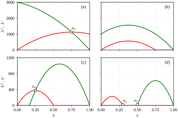
Figure 1: Four different regimes of the model observed by comparing the birth (green curve) and the death (red curve) transition rates, Eq. (8). Open circles mark fixed points of the model. Model parameters: $N=10^{3}$, $h=1$, $\sigma_{0}=2$, $\sigma_{1}=4$, $\alpha=\beta=1$ (all cases), $q=1$ (a), $3$ (b), $5$ (c) and $9$ (d).

The transition points between these regimes, or the critical points, are found whenever both rates go to zero at the same $X$. Thus the critical points can be determined by solving the following system of equations

$$\begin{cases}\lambda^{+}\left(xN\right)=0\\ \lambda^{-}\left(xN\right)=0\end{cases},$$ (10)

in respect to $x$ and $q$. While solving Eq. (10) we treat the special brackets $\left[z\right]_{+}$ as if they were ordinary ones. With this caveat we obtain three solutions of Eq. (10):

$$x_{1}=0 ,\quad q_{1}=N^{\beta-1}\sigma_{1},$$ (11)

$$x_{2}=1 ,\quad q_{2}=N^{\beta-1}\sigma_{0},$$ (12)

$$x_{3}=\frac{Nh+N^{\alpha}\sigma_{0}}{2Nh+N^{\alpha}\left(\sigma_{0}+\sigma_{1}\right)} ,\quad q_{3}=N^{\beta-\alpha-1}\left(Nh+N^{\alpha}\left(\sigma_{0}+\sigma_{1}\right)\right).$$ (13)

Note that $q_{3}$ will be always larger than $q_{1}$ and $q_{2}$. Therefore the the third critical point, $q_{c,3}$, corresponds to $q_{3}$. The first two critical points correspond to $q_{1}$ and $q_{2}$. Which of them is smaller depends on the selected values of $\sigma_{0}$ and $\sigma_{1}$. For the asymmetric case, $\sigma_{0}\neq\sigma_{1}$, we have:

$$q_{c,1} =N^{\beta-1}\min\left(\sigma_{0},\sigma_{1}\right),\quad q_{c,2}=N^{\beta-1}\max\left(\sigma_{0},\sigma_{1}\right).$$ (14)

In the symmetric case, $\sigma_{0}=\sigma_{1}$, we have $q_{1}=q_{2}$ and thus the second regime would not be observed.

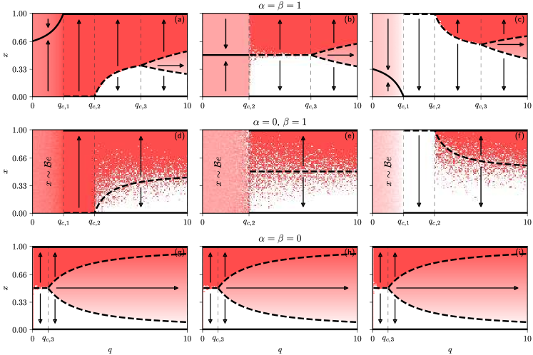
Figure 2: Bifurcation diagrams of the model driven by Eq. (8) in respect to the intensity of support, $q$. Black curves correspond to stable fixed points (solid curves) and unstable fixed points (dashed curves). Arrows indicate directions in which the model moves. Areas are shaded according to the value of $x$ reached after sufficiently long time (white corresponds to $x\left(t\right)=0$, red corresponds to $x\left(t\right)=1$, while shades correspond to some intermediate values). Model parameters used to produce this figure: $N=10^{3}$ and $h=1$ (all cases), $\sigma_{0}=2$ and $\sigma_{1}=4$ ((a), (d) and (g)), $\sigma_{0}=\sigma_{1}=3$ ((b), (e) and (h)), $\sigma_{0}=4$ and $\sigma_{1}=2$ ((c), (f) and (i)), $\alpha=\beta=1$ ((a)–(c)), $\alpha=0$ and $\beta=1$ ((d)–(f)), $\alpha=\beta=0$ ((g)–(i)).

In Fig. 2 we have shown the dependence of the fixed points on intensity of support, $q$, in the model driven by Eq. (8). We have considered extensive ($\alpha=\beta=1$), non–extensive ($\alpha=\beta=0$) and hybrid ($\alpha=0$ and $\beta=1$) interaction cases. The extensive case and the non–extensive case assume that all agents interact in the same manner (either extensive or non–extensive), while the hybrid case assumes that the agents in different state (opposition) have more influence. Assuming the opposite, that allies have more influence (i.e., setting $\alpha=1$ and $\beta=0$), might be a more reasonable assumption in the opinion dynamics context, but it leads to a trivial model as both rates quickly go to zero with larger $N$.

Let us continue with a discussion of Fig. 2 and obtain the expressions for the fixed points. For $q<q_{c,1}$ we observe either a stable fixed point or a stationary distribution. Stable fixed point $x_{s}$, which is observed only for $\alpha=\beta=1$, has to satisfy:

$$\lambda^{+}\left(x_{s}N\right)=\lambda^{-}\left(x_{s}N\right).$$ (15)

This fixed point was highlighted in Fig. 1 (a). We once again treat the special brackets $\left[z\right]_{+}$ as if they were ordinary and obtain:

$$x_{s}=\frac{q-\sigma_{1}}{2q-\left(\sigma_{0}+\sigma_{1}\right)}.$$ (16)

For $\alpha=0$ and finite $N$ we observe the Beta–binomial distribution, in the infinite $N$ limit the stationary distribution converges to the Beta distribution:

$$x\sim\mathcal{B}e\left(\frac{\sigma_{1}-qN^{1-\beta}}{h+qN^{-\beta}},\frac{\sigma_{0}-qN^{1-\beta}}{h+qN^{-\beta}}\right).$$ (17)

Earlier works [30, 31] have already observed the emergence of the stationary Beta distribution in the non–extensive voter model ($\alpha=0$ and $q=0$) and its convergence to the Dirac delta function as $\alpha\rightarrow 1$ and $N\rightarrow\infty$. The result we have obtained here complements the previous knowledge and shows that the stationary distribution can be also observed for $q>0$. Furthermore the result has an interesting implication from opinion dynamics perspective. Namely, a society of independent (informed or educated) individuals who provide strong support for their peers can be statistically indistinguishable from a society thriving on imitation (with individuals being uninformed or badly educated).

In all asymmetric cases the second regime is observed. In the second regime, for $q_{c,1}<q<q_{c,2}$, we observe fixed points at $x=0$ and $x=1$: one of them being stable, the other being unstable. Which is which depends on the parameters $\sigma_{0}$ and $\sigma_{1}$. If $\sigma_{0}<\sigma_{1}$, then $x=1$ is the stable fixed point and $x=0$ is the unstable fixed point. In the opposite case, $\sigma_{0}>\sigma_{1}$, $x=0$ is the stable fixed point and $x=1$ is the unstable fixed point.

Special transitional regime is observed for $\alpha=\beta=1$ with $\sigma_{0}=\sigma_{1}=q$. In this case the model does not experience drift, only diffusion is present if $N$ is finite. Therefore for finite $N$ the model randomly diffuses until it sticks to either $x=0$ or $x=1$. In the infinite $N$ limit diffusion function also goes to zero and all points become stable.

In all cases for $q_{c,2}<q<q_{c,3}$ we observe two ordered phases are separated by an unstable fixed point. This unstable fixed point $x_{u}$ has to satisfy:

$$\lambda^{+}\left(x_{u}N\right)=\lambda^{-}\left(x_{u}N\right).$$ (18)

This fixed point was highlighted in Fig. 1 (c). We once again treat the special brackets $\left[z\right]_{+}$ as if they were ordinary and obtain:

$$x_{u}=\frac{Nq-N^{\beta}\sigma_{1}}{2Nq-N^{\beta}\left(\sigma_{0}+\sigma_{1}\right)}.$$ (19)

Note that this expression is similar to the one obtained for $x_{s}$, only the considered $q$ value range is different. Indeed if we set $\beta=1$, we would obtain exactly the same expression as in Eq. (16).

For $\alpha=0$ the separation between the phases is not deterministic, but probabilistic instead. This is because in this case the contribution of diffusion is non–negligible even if we take infinite $N$ limit. Therefore a process starting below $x_{u}$ has a non–zero probability to be absorbed at $x=1$. The opposite, process starting above $x_{u}$ and being absorbed at $x=0$ with non–zero probability, is also true in this case. Therefore the numerical results shown in Fig. 2 appear to be somewhat scattered. Especially around the $x_{u}$ curve.

In all cases for $q_{c,3}<q$ we observe a set of stable fixed points in the middle (marked by the right arrow in Fig. 2). The boundaries of this region are obtained by solving

$$\lambda^{+}\left(x_{\uparrow}N\right)=0\quad\mbox{and}\quad\lambda^{-}\left(x_{\downarrow}N\right)=0.$$ (20)

These points were highlighted in Fig. 1 (d). We once again treat the special brackets $\left[z\right]_{+}$ as if they were ordinary and obtain the following non–trivial solutions for the respective equations:

$$x_{\uparrow} =\frac{q-N^{\beta-1}\sigma_{1}}{q+N^{\beta-\alpha}h},\quad x_{\downarrow}=\frac{h+N^{\alpha-1}\sigma_{0}}{h+N^{\beta-\alpha}q}.$$ (21)

Note that these points are also unstable fixed points.

It is worth to note that not all critical points and regimes are visible in Fig. 2. In all three cases for $\sigma_{0}=\sigma_{1}$ we have $q_{c,1}=q_{c,2}$ and we show just $q_{c,2}$ in the figure. For $\alpha=0$ and $\beta=1$ in the infinite $N$ limit $q_{c,3}$ goes to infinity. Even for finitely large $N$ it would be hard to justify values of $q$ of the order of $q_{c,3}$. Similarly for $\beta=0$ both $q_{c,1}$ and $q_{c,2}$ go to zero in the infinite $N$ limit and are not shown in Fig. 2.

Qualitatively bifurcation diagrams of the model driven by (8) are quite similar to each other. It appears that both the hybrid case and the non–extensive case have bifurcation diagrams, which are essentially appropriately stretched bifurcation diagram for the case $\alpha=\beta=1$. There is just a single major exception for $q<q_{c,1}$ in $\alpha=0$ and $\beta=1$ case. In this case the model converges not to a fixed point, but to a stationary distribution. Note that this regime would be alsp observed in $\alpha=\beta=0$ case, but in this case $q_{c,1}\rightarrow 0$ as $N\rightarrow\infty$.

4 Support deterring imitation

Now let us assume that support provided by the allies discourages only imitation. This means that independent behavior is not affected by the support and the transition rates take the following form:

$$\lambda_{p}^{+} =\left(N-X\right)\left(\sigma_{1}+\left[\frac{h}{N^{\alpha}}X-\frac{q}{N^{\beta}}\left(N-X\right)\right]_{+}\right),$$

$$\lambda_{p}^{-} =X\left(\sigma_{0}+\left[\frac{h}{N^{\alpha}}\left(N-X\right)-\frac{q}{N^{\beta}}X\right]_{+}\right).$$ (22)

To supplement further discussion on the fixed points of this model let us find the zeros of the special brackets:

$$\frac{h}{N^{\alpha}}Nx^{+}-\frac{q}{N^{\beta}}N\left(1-x^{+}\right)=0,\quad \Rightarrow\quad x^{+}=\frac{N^{\alpha}q}{N^{\beta}h+N^{\alpha}q},$$ (23)

$$\frac{h}{N^{\alpha}}N\left(1-x^{-}\right)-\frac{q}{N^{\beta}}Nx^{-}=0,\quad \Rightarrow\quad x^{-}=\frac{N^{\beta}h}{N^{\beta}h+N^{\alpha}q}.$$ (24)

We can introduce the four types of fixed points in relation to these roots. An example with three types of fixed points is provided in Fig. 3.

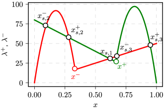
Figure 3: Roots of the special brackets (colored circles) and fixed points (black circles) of the model driven by Eq. (22). Green curve correspond to the birth rate (green curve), while red the death (red curve) rates. Assumed model parameters: $N=1000$, $\alpha=\beta=1$, $h=1$, $\sigma_{0}=0.05$, $\sigma_{1}=0.08$.

Fixed point of the first type is found when both of the special brackets evaluate to zero, namely if $x^{-}\leq x_{s,1}\leq x^{+}$. As the special brackets are zero, the fixed point is obtained by solving:

$$\left(1-x_{s,1}\right)\sigma_{1}=x_{s,1}\sigma_{0}\quad\Rightarrow\quad x_{s,1}=\frac{\sigma_{1}}{\sigma_{0}+\sigma_{1}}.$$ (25)

This fixed point is stable whenever it is observed. Fixed point of the first type and fixed point of the fourth type are mutually exclusive.

Fixed points of the second and third types are found when one of the special brackets evaluates to zero. Therefore we have the following conditions $x_{s,2}^{\pm}<x^{+}\land x_{s,2}^{\pm}<x^{-}$ and $x_{s,3}^{\pm}>x^{+}\land x_{s,3}^{\pm}>x^{-}$ to observe the respective fixed points. The equations to find fixed points of the second and third types are given by:

$$N\left(1-x\right)x_{s,2} =\lambda_{p}^{-}\left(x_{s,2}N\right),$$ (26)

$$\lambda_{p}^{+}\left(x_{s,3}N\right) =Nx_{s,3}\sigma_{0}.$$ (27)

We treat the remaining special brackets as if they were ordinary brackets and obtain the following solutions to these equations:

$$x_{s,2}^{\pm} =\frac{A\pm\sqrt{A^{2}-2B\sigma_{1}}}{B},$$ (28)

$$x_{s,3}^{\pm} =\frac{A+2\left(N^{1-\beta}q-\sigma_{0}-\sigma_{1}\right)\pm\sqrt{A^{2}-2B\sigma_{0}}}{B}.$$ (29)

Here we have introduced shorthands for expressions which repeat in the obtained solutions:

$$A=N^{1-\alpha}h+\sigma_{0}+\sigma_{1},\quad B=2N\left(N^{-\alpha}h+N^{-\beta}q\right).$$ (30)

For the fixed points of the second type smaller solution is stable and the larger one is unstable, while for the fixed points of the third type larger solution is stable and the smaller one is unstable.

Fixed point of the fourth type is found when both of the special brackets are positive, namely if $x^{+}\leq x_{s,4}\leq x^{-}$. The respective equation is given by:

$$\lambda_{p}^{+}\left(x_{s,4}N\right)=\lambda_{p}^{-}\left(x_{s,4}N\right).$$ (31)

Here we treat the special brackets as if they were ordinary ones and obtain:

$$x_{s,4}=\frac{Nq-N^{\beta}\sigma_{1}}{2Nq-N^{\beta}\left(\sigma_{0}+\sigma_{1}\right)}.$$ (32)

This fixed point might be stable or unstable depending on the shapes of the transition rates. Besides the discussed conditions all of the fixed points must be real and within $\left[0,1\right]$ interval. Following this discussion one could provide closed form expressions for the critical points as well as conditions for their existence. Yet those expressions are rather lengthy and complicated, while the intuition they provide is very simple and can be shown visually (see Figs. 4, 5 and 6).

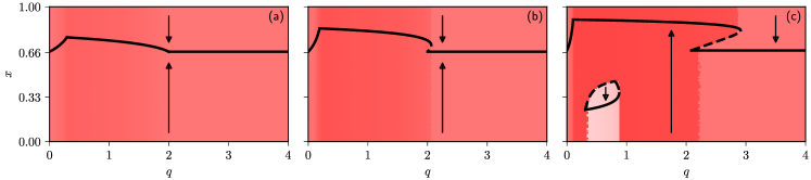
Figure 4: Bifurcation diagrams of the model driven by Eq. (22) in respect to the intensity of support $q$ in the extensive ($\alpha=\beta=1$) interaction case. Black curves correspond to stable fixed points (solid curves) and unstable fixed points (dashed curves). Arrows indicate directions in which the model moves. Areas are shaded according to the value of $x$ reached after sufficiently long time (white corresponds to $x\left(t\right)=0$, red corresponds to $x\left(t\right)=1$, while shades correspond to some intermediate values). Model parameters: $N=10^{3}$, $h=1$ (all cases), $\sigma_{0}=0.5$ and $\sigma_{1}=1$ (a), $\sigma_{0}=0.25$ and $\sigma_{1}=0.5$ (b), $\sigma_{0}=0.12$ and $\sigma_{1}=0.25$ (c).

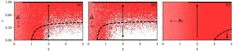
Figure 5: Bifurcation diagrams of the model driven by Eq. (22) in respect to the intensity of support $q$ in the hybrid ($\alpha=0$ and $\beta=1$) interaction case. Black curves correspond to stable fixed points (solid curves) and unstable fixed points (dashed curves). Arrows indicate directions in which the model moves. Areas are shaded according to the value of $x$ reached after sufficiently long time (white corresponds to $x\left(t\right)=0$, red corresponds to $x\left(t\right)=1$, while shades correspond to some intermediate values). Model parameters: $N=10^{3}$, $h=1$ (all cases), $\sigma_{0}=0.5$ and $\sigma_{1}=1$ (a), $\sigma_{0}=0.5$ and $\sigma_{1}=0.25$ (b), $\sigma_{0}=1.5$ and $\sigma_{1}=3$ (c).

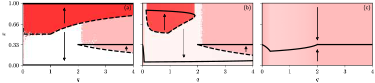
Figure 6: Bifurcation diagrams of the model driven by Eq. (22) in respect to the intensity of support $q$ in the non–extensive ($\alpha=\beta=0$) interaction case. Black curves correspond to stable fixed points (solid curves) and unstable fixed points (dashed curves). Arrows indicate directions in which the model moves. Areas are shaded according to the value of $x$ reached after sufficiently long time (white corresponds to $x\left(t\right)=0$, red corresponds to $x\left(t\right)=1$, while shades correspond to some intermediate values). Model parameters: $N=10^{3}$, $h=1$ (all cases), $\sigma_{0}=1$ and $\sigma_{1}=0.5$ (a), $\sigma_{0}=120$ and $\sigma_{1}=60$ (b), $\sigma_{0}=10^{3}$ and $\sigma_{1}=500$ (c).

As in the previous section we observe that the bifurcation diagrams of the model driven by Eq. (22) are qualitatively the same for all three considered cases. The bifurcation diagrams appear to be just the rescaled versions of each other. For large $\sigma_{i}$ only one stable fixed point is observed (as can be seen in Fig. 4 (a) or Fig. 6 (c)). As $\sigma_{i}$ becomes smaller an unstable fixed point emerges to act as a separator between two stable fixed points (see Fig. 4 (b)). As $\sigma_{i}$ becomes even smaller another pair of stable and unstable fixed points emerges (see Fig. 4 (c)). Further decreasing $\sigma_{i}$ triggers emergence of a regime with five fixed points (see Fig. 6 (b) and (a)).

For the hybrid interaction case, Fig. 5, we observe regime, for $q<\min\left(\sigma_{0},\sigma_{1}\right)$, in which the model is converges not to a fixed point, but to a stationary distribution. The same regime is observed for the non–extensive interaction case, too, but in the infinite $N$ limit this regime disappears completely as $q<\min\left(\sigma_{0},\sigma_{1}\right)/N$ must hold for the regime to be observed. In both cases the stationary distribution is the Beta distribution (Beta–binomial for finite $N$) with the following parameters:

$$x\sim\mathcal{B}e\left(\frac{\sigma_{1}-qN^{1-\beta}}{h+qN^{-\beta}},\frac{\sigma_{0}-qN^{1-\beta}}{h+qN^{-\beta}}\right).$$ (33)

The stationary distribution is exactly the same as for the model from the previous section.

For the hybrid interaction case, Fig. 5, we also observe some deviations from the expected behavior. These deviations are caused by a strong diffusion, which is able to overcome influence of drift for the smaller $q$ values. Strong diffusion allows trajectories to escape smaller basins of attraction. Usually those smaller basins attract to the state having smaller $\sigma_{i}$.

As previously we observe special transitional regime for the extensive interaction case with $\sigma_{0}=\sigma_{1}=q$. But for this model the drift function goes to zero for $x^{+}\leq x\leq x^{-}$, while the trajectories starting outside this interval are attracted to $x^{+}$ or $x^{-}$. For finite $N$ trajectories meander inside the interval, but in the infinite $N$ limit all the points inside the interval become stable.

5 Conclusions

We have conducted a thorough analysis of the noisy voter model with supportive interactions. We have considered two different ways to implement supportive interactions. In the first considered model the support discourages both independent and peer pressure induced transitions. In the second model we have assumed that the support discourages only peer pressure induced transitions. In the first model supportive independent agents (society of educated people) effectively behave as ordinary imitative agents (society of uneducated people). Namely the first model is often driven to full consensus state. Unless support is extremely strong, in that case polarized states become stable. In contrast the second model allows partial consensus states to be stable fixed points. For certain parameter sets there are multiple stable fixed points corresponding to partial consensus states in the second model.

We have considered both of these models in different agent interaction scenarios: extensive, non–extensive and hybrid. The extensive and the non–extensive interaction scenarios were already explored in [38, 39, 31]. It was shown that the extensive interactions lead to a macroscopic description by an ODE (thus the extensive noisy voter model converges to a fixed point) and the non–extensive interactions lead to a macroscopic description by an SDE (thus the non–extensive noisy voter model converges to a stationary distribution). Introducing supportive interactions into the non–extensive noisy voter model increases impact of drift and makes diffusion negligible by comparison. Therefore the modified non–extensive model is approximated by an ODE and converges to a fixed point. Stationary distribution is observed only in the hybrid interaction scenario (interactions with the opposition are non–extensive, while interactions with allies are extensive) when support is weak.

There are other ways to model support in context of the noisy voter model. One of the possibilities is to have supportiveness depend on the current system state (i.e., becoming stronger if a group is in minority). Impact of support could be studied in the $q$-voter model, which is well–known generalization of the voter model [12, 16]. Similarity with non–Markovian opinion freezing models [34, 35, 36, 37] prompts a question to which extent the supportive interactions with past selves (memory) is equivalent to the supportive interactions among peers, providing grounds for further inquiry into the nature of spurious long–range memory [48, 49]. It might be reasonable to model support using the complex contagion framework [15], which would provide a more transparent view of pairwise interactions between agents in real time.

References

- [1] R. Axelrod, The dissemination of culture a model with local convergence and global polarization, Journal of Conflict Resolution 41 (2) (1997) 203–226. doi:10.1177/0022002797041002001.
- [2] A. Flache, M. Mas, T. Feliciani, E. Chattoe-Brown, G. Deffuant, S. Huet, J. Lorenz, Models of social influence: Towards the next frontiers, The Journal of Artificial Society and Social Simulation 20 (4) (2017) 2. doi:10.18564/jasss.3521.
- [3] A. R. Binder, K. E. Dalrymple, D. Brossard, D. A. Scheufele, The soul of a polarized democracy: Testing theoretical linkages between talk and attitude extremity during the 2004 presidential election, Communication Research 36 (3) (2009) 315–340. doi:10.1177/0093650209333023.
- [4] S. Galam, Public debates driven by incomplete scientific data: The cases of evolution theory, global warming and H1N1 pandemic influenza, Physica A 389 (17) (2010) 3619 – 3631. doi:10.1016/j.physa.2010.04.039.
- [5] A. M. McCright, R. E. Dunlap, The politicization of climate change and polarization in the american public’s views of global warming, 2001–2010, The Sociological Quarterly 52 (2) (2011) 155–194. doi:10.1111/j.1533-8525.2011.01198.x.
- [6] A. L. Schmidt, F. Zollo, A. Scala, C. Betsch, W. Quattrociocchi, Polarization of the vaccination debate on facebook, Vaccine 36 (25) (2018) 3606 – 3612. doi:10.1016/j.vaccine.2018.05.040.
- [7] B. W. Hardy, M. Tallapragada, J. C. Besley, S. Yuan, The effects of the "War on Science" frame on scientists’ credibility, Science Communication 41 (1) (2019) 90–112. doi:10.1177/1075547018822081.
- [8] H. R. Willis, Conformity, independence and anticonformity, Human Relations 18 (1965) 373. doi:10.1177/001872676501800406.
- [9] B. Latane, The psychology of social impact, American Psychologist 36 (4) (1981) 343–356. doi:10.1037/0003-066X.36.4.343.
- [10] G. Akerlof, J. Shiller, Animal spirits: How human psychology drives the economy, and why it matters for global capitalism, Princeton University Press, 2009.
- [11] D. G. Lilleker, Modelling political cognition, Palgrave Macmillan UK, London, 2014, pp. 198–205.
- [12] C. Castellano, S. Fortunato, V. Loreto, Statistical physics of social dynamics, Reviews of Modern Physics 81 (2009) 591–646. doi:10.1103/RevModPhys.81.591.
- [13] D. Stauffer, A biased review of sociophysics, Journal of Statistical Physics 151 (2013) 9–20. doi:10.1007/s10955-012-0604-9.
- [14] F. Abergel, H. Aoyama, B. Chakrabarti, A. Chakraborti, N. Deo, D. Raina, I. Vodenska (Eds.), Econophysics and sociophysics: Recent progress and future directions, Springer, 2017.
- [15] A. Baronchelli, The emergence of consensus: a primer, Royal Society Open Science 5 (2018) 172189. doi:10.1098/rsos.172189.
- [16] A. Jedrzejewski, K. Sznajd-Weron, Statistical physics of opinion formation: Is it a SPOOF?, Comptes Rendus Physique 20 (4) (2019) 244–261. doi:10.1016/j.crhy.2019.05.002.
- [17] S. Redner, Reality inspired voter models: a mini-review, Comptes Rendus Physique 20 (4) (2019) 275–292, available as arXiv:1811.11888 [physics.soc-ph]. doi:10.1016/j.crhy.2019.05.004.
- [18] M. Galesic, D. L. Stein, Statistical physics models of belief dynamics: Theory and empirical tests, Physica A 519 (2019) 275–294. doi:10.1016/j.physa.2018.12.011.
- [19] A. Kononovicius, Empirical analysis and agent-based modeling of Lithuanian parliamentary elections, Complexity 2017 (2017) 7354642. doi:10.1155/2017/7354642.
- [20] P. Bancerowski, K. Malarz, Multi-choice opinion dynamics model based on Latane theory, European Physical Journal B 92 (2019) 219. doi:10.1140/epjb/e2019-90533-0.
- [21] F. Vazquez, E. S. Loscar, G. Baglietto, A multi-state voter model with imperfect copying, Physical Review E 100 (2019) 042301, available as 1902.07253 [physics.soc-ph]. doi:10.1103/PhysRevE.100.042301.
- [22] P. Clifford, A. Sudbury, A model for spatial conflict, Biometrika 60 (1973) 581 – 588. doi:10.1093/biomet/60.3.581.
- [23] T. Liggett, Stochastic interacting systems: Contact, voter, and exclusion processes, Springer, 1999.
- [24] L. B. Granovsky, N. Madras, The noisy voter model, Stochastic Processes and their Applications 55 (1) (1995) 23–43. doi:10.1016/0304-4149(94)00035-R.
- [25] M. Mobilia, A. Petersen, S. Redner, On the role of zealotry in the voter model, Journal of Statistical Mechanics: Theory and Experiment 2007 (08) (2007) P08029. doi:10.1088/1742-5468/2007/08/p08029.
- [26] N. Khalil, M. San Miguel, R. Toral, Zealots in the mean-field noisy voter model, Physical Review E 97 (2018) 012310. doi:10.1103/PhysRevE.97.012310.
- [27] S. Tanabe, N. Masuda, Complex dynamics of a nonlinear voter model with contrarian agents, Chaos 23 (2013) 043136. doi:10.1063/1.4851175.
- [28] T. Krueger, J. Szwabinski, T. Weron, Conformity, anticonformity and polarization of opinions: Insights from a mathematical model of opinion dynamics, Entropy 2017 (19) (2017) 371. doi:10.3390/e19070371.
- [29] N. Khalil, R. Toral, The noisy voter model under the influence of contrarians, Physica A 515 (2019) 81–92. doi:https://doi.org/10.1016/j.physa.2018.09.178.
- [30] S. Alfarano, M. Milakovic, Network structure and N-dependence in agent-based herding models, Journal of Economic Dynamics and Control 33 (1) (2009) 78–92. doi:10.1016/j.jedc.2008.05.003.
- [31] A. Kononovicius, J. Ruseckas, Continuous transition from the extensive to the non-extensive statistics in an agent-based herding model, European Physics Journal B 87 (8) (2014) 169. doi:10.1140/epjb/e2014-50349-0.
- [32] C. Castellano, M. A. Munoz, R. Pastor-Satorras, The non-linear q-voter model, Physical Review E 80 (2009) 041129. doi:10.1103/PhysRevE.80.041129.
- [33] A. F. Peralta, A. Carro, M. San Miguel, R. Toral, Analytical and numerical study of the non-linear noisy voter model on complex networks, Chaos 28 (2018) 075516. doi:10.1063/1.5030112.
- [34] H.-U. Stark, C. J. Tessone, F. Schweitzer, Decelerating microdynamics can accelerate macrodynamics in the voter model, Physical Review Letters 101 (2008) 018701. doi:10.1103/PhysRevLett.101.018701.
- [35] H.-U. Stark, C. J. Tessone, F. Schweitzer, Slower is faster: Fostering consensus formation by heterogeneous inertia, Advances in Complex Systems 11 (04) (2008) 551–563. doi:10.1142/s0219525908001805.
- [36] Z. Wang, Y. Liu, L. Wang, Y. Zhang, Z. Wang, Freezing period strongly impacts the emergence of a global consensus in the voter model, Scientific Reports 4 (1) (2014). doi:10.1038/srep03597.
- [37] O. Artime, A. F. Peralta, R. Toral, J. Ramasco, M. San Miguel, Aging-induced continuous phase transition, Physical Review E 98 (2018) 032104. doi:10.1103/PhysRevE.98.032104.
- [38] S. Alfarano, T. Lux, F. Wagner, Estimation of agent-based models: The case of an asymmetric herding model, Computational Economics 26 (1) (2005) 19–49. doi:10.1007/s10614-005-6415-1.
- [39] S. Alfarano, T. Lux, F. Wagner, Time variation of higher moments in a financial market with heterogeneous agents: An analytical approach, Journal of Economic Dynamics and Control 32 (2008) 101–136. doi:10.1016/j.jedc.2006.12.014.
- [40] A. Kononovicius, V. Gontis, Agent based reasoning for the non-linear stochastic models of long-range memory, Physica A 391 (4) (2012) 1309–1314. doi:10.1016/j.physa.2011.08.061.
- [41] V. Gontis, A. Kononovicius, Consentaneous agent-based and stochastic model of the financial markets, PLoS ONE 9 (7) (2014) e102201. doi:10.1371/journal.pone.0102201.
- [42] T. Lux, Estimation of agent-based models using sequential Monte Carlo methods, Journal of Economic Dynamics and Control 91 (2018) 391–408. doi:10.1016/j.jedc.2018.01.021.
- [43] P. R. Nail, K. Sznajd-Weron, The diamond model of social response within an agent-based approach, Acta Physica Polonica A 129 (5) (2016) 1050–1054. doi:10.12693/APhysPolA.129.1050.
- [44] A. Nowak, J. Szamrej, B. Latane, From private attitude to public opinion: A dynamic theory of social impact., Psychological Review 97 (3) (1990) 362. doi:10.1037/0033-295X.97.3.362.
- [45] M. J. de Oliveira, Isotropic majority-vote model on a square lattice, Journal of Statistical Physics (1992). doi:10.1007/BF01060069.
- [46] A. L. M. Vilela, H. E. Stanley, Effect of strong opinions on the dynamics of the majority-vote model, Scientific Reports 8 (2018) 8709. doi:10.1038/s41598-018-26919-y.
- [47] N. G. van Kampen, Stochastic process in physics and chemistry, North Holland, Amsterdam, 2007.
- [48] L. Charfeddine, A varieties of spurious long memory process, IJBSS 2 (3) (2011) 52–66. URL: http://ijbssnet.com/journals/Vol._2_No._3_[Special_Issue_-_January_2011]/5.pdf
- [49] V. Gontis, A. Kononovicius, Spurious memory in non-equilibrium stochastic models of imitative behavior, Entropy 19 (8) (2017) 387. doi:10.3390/e19080387.