An extended theoretical scenario for Classical Cepheids. I. Modeling Galactic Cepheids in the Gaia photometric system

Abstract

We present a new extended and detailed set of models for Classical Cepheid pulsators at solar chemical composition ($Z=0.02$, $Y=0.28$) based on a well tested nonlinear hydrodynamical approach. In order to model the possible dependence on crucial assumptions such as the Mass-Luminosity relation of central Helium burning intermediate-mass stars or the efficiency of superadiabatic convection, the model set was computed by varying not only the pulsation mode and the stellar mass but also the Mass-Luminosity relation and the mixing length parameter that is used to close the system of nonlinear hydrodynamical and convective equations. The dependence of the predicted boundaries of the instability strip as well as of both light and radial velocity curves on the assumed Mass-Luminosity and the efficiency of superadiabatic convection is discussed. Nonlinear Period-Mass-Luminosity-Temperature, Period-Radius and Period-Mass-Radius relations are also computed. The theoretical atlas of bolometric light curves for both the fundamental and first overtone mode has been converted in the Gaia filters $G$, $G_{BP}$ and $G_{BR}$ and the corresponding mean magnitudes have been derived. Finally the first theoretical Period-Luminosity-Color and Period-Wesenheit relations in the Gaia filters are provided and the resulting theoretical parallaxes are compared with Gaia Data Release 2 results for both fundamental and first overtone Galactic Cepheids.

1 Introduction

Classical Cepheids (CC) are pulsating intermediate-mass central Helium burning stars associated to the blue loop phase in the Color-Magnitude diagram. Their characteristic Period-Luminosity (PL) and Period-Luminosity-Color (PLC) relations make these objects excellent distance indicators in the Local Group and beyond. Thanks to the capability of the Hubble Space Telescope (HST, see e.g. Freedman et al., 2001; Riess et al., 2011) the Cepheid distance scale has been extended up to almost 30 Mpc and still longer distances will be covered with the next generation observetional facilities, such as the Extremely Large Telescope from the ground or the James Webb Space Telescope from the space.

From the calibration of secondary distance indicators based on Cepheids in the Milky Way, the LMC, and the maser HST galaxy NGC 4258, Riess et al. (2019) derived a value of the Hubble Constant ($H_{0}=$ 74.03$\pm$ 1.42 $kms^{-1}Mpc^{-1}$) that is systematically higher than the value ($H_{0}=$ 67.4$\pm$0.5 $kms^{-1}Mpc^{-1}$) based on the investigation of the Cosmic Microwave Background (CMB, Planck Collaboration et al., 2018). The significant discrepancy between the two estimated values of $H_{0}$ is known as ’The Hubble Constant tension’. In this context it is worth investigating possible residual sources of uncertainties affecting the Cepheid-based extragalactic distance scale. We know that Cepheid PL and PLC relations may be affected by metallicity corrections. Even if this effect has been accounted for in Riess et al. derivation, several authors provide different metallicity corrections (e.g. Macri et al. (2006); Romaniello et al. (2008); Marconi et al. (2005)), in some cases partially balanced by theoretically predicted Helium abundance effects (e.g. Carini et al. (2014); Marconi et al. (2005)) and there is no general consensus in the literature. But even neglecting the metallicity problem, the theory of stellar evolution and pulsation predicts that other effects can change the coefficients of the above mentioned relations. These are for example the efficiency of superadiabatic convection, that contributes to the quenching of pulsation which affects the topology of the instability strip as well as the pulsation amplitudes, or the actual Mass-Luminosity (ML) relation predicted by stellar evolution models for CC which is well known to depend on nonstandard physical phenomena such as core-overshooting, mass loss and rotation.

In order to quantify these effects on the predicted Cepheid distance scale we started a theoretical project aiming at building a complete grid of nonlinear convective pulsation models spanning simultaneously a range of possible ML relations, superadiabatic convection efficiencies and chemical compositions. The final goal is to provide an extensive and detailed pulsation model database to complement similar sets of evolutionary models (see e.g. BaSTI database, PISA stellar models, Padova database of stellar evolutionary tracks and isochrones) available to the astrophysical community.

This paper, devoted to the first completed model set at solar chemical composition (Z=0.02 Y=0.28), represents the first step in this direction, whereas the extension to other chemical compositions will be presented in a forthcoming work (De Somma et al. in prep).

In this context, the Gaia mission (Gaia Collaboration et al., 2016) is producing a 3D-map of 1 billion stars of the Milky Way with unprecedented accuracy. Focusing on pulsating stars, after the recent Data Release 2 (Gaia Collaboration et al., 2018; Holl et al., 2018), a large sample of Cepheids, observed in three photometric bands ($G$, $G_{BP}$ and $G_{RP}$) complemented with accurate parallaxes and proper motions, is available to the scientific community (Clementini et al., 2019; Ripepi et al., 2019), and the future releases will provide also radial velocity time series. This important database represents a challenging benchmark for testing the physical and numerical assumptions of current pulsation models. On this basis, in this paper we provide the first set of predicted light curves in the Gaia filters together with the associated mean magnitudes and colors and in turn the inferred PLC and Period-Wesenheit (PW) relations in the Gaia photometric system.

The organization of the paper is the following: in Section 2 we present the set of pulsation models; in Section 3 we derive the pulsation relation connecting the period to the intrinsic stellar parameters, the predicted instability strip and the theoretical atlas of light and radial velocity curves, including the effects of the assumed ML and superadiabatic convective efficiency. Moreover, we estimate the Period-Radius (PR) and Period-Mass-Radius (PMR) relations as a function of the above mentioned assumptions and make a comparison with independently derived PR relations in the literature; in Section 4 we provide the first theoretical light curves in the Gaia photometric system from which we obtain mean magnitudes and colors and the first PLC and the PW relations in the Gaia filters; in Section 5 we derive theoretical parallaxes based on the PW relations in the Gaia filters and make a comparison between theoretical and Gaia Data Release 2 (DR2) parallaxes; in Section 6 the conclusions close the paper.

2 The extended set of pulsation models

In order to compute the extended set of Cepheid nonlinear convective pulsation models we adopte the hydrodynamical code and the physical and numerical assumptions discussed in Bono et al. (2000a, b); Marconi et al. (2013a, 2010); but a new automatized procedure has been developed to compute extended model sets, with unprecedented fine input parameter grids. These models have solar metallicity $Z=0.02$ and Helium content $Y=0.28$ and span a wide range of masses (3 $\leq$ $\frac{M}{M_{\odot}}$ $\leq$ 11) and temperatures ($3600$K $\leq$ $T_{eff}$ $\leq$ $6700K$). For each selected stellar mass, three luminosity levels are considered: a canonical level (named A), based on stellar evolution predictions that neglect mass loss, rotation and core overshooting (Bono et al., 2000b) and two noncanonical luminosity levels obtained by increasing the canonical luminosity level by 0.2 dex (named B) and 0.4 dex (named C), respectively. Moreover, in order to investigate the effect of superadiabatic convection efficiency, whose known main effect is to quench the pulsation driving mechanism, each selected model is computed for three values of the mixing length parameter $\alpha~{}$=$~{}l/H_{P}$ adopted to close the system of nonlinear hydrodynamical and convective equations (Bono et al., 1999), namely $\alpha=1.5$ , $\alpha=1.7$ and $\alpha=1.9$. The choice of the mixing length parameter range was based on specific computations presented in previous papers (Di Criscienzo et al. (2004); Fiorentino et al. (2007); Natale et al. (2008); Marconi et al. (2013a)) which suggested that hotter variables are well reproduced with $\alpha$ = 1.5-1.6, whereas variables closer to the red edge of the instability strip often enquire $\alpha$ = 1.8-2.0 due to the most important efficiency of convection in the redder part of the color-magnitude diagram.

For each pulsation model the nonlinear equations are integrated until a stable limit cycle is attained in the F or FO mode. Table LABEL:f_param_model and Table LABEL:fo_param_model report the intrinsic stellar parameters for the computed F and FO models, respectively. Columns from 1 to 5 report the stellar mass, the luminosity level, the effective temperature, the adopted mixing length parameter, the luminosity level identification defined above. The pulsation period and the average radius inferred from the application of the nonlinear convective code are listed in the last 2 columns.

Stellar mass (solar units).

Logarithmic luminosity (solar units).

Effective temperature (K).

Mixing length parameter.

Mass-Luminosity relation.

Period (days).

Logarithmic mean radius (solar units).

Table 1: The intrinsic stellar parameters for computed F mode models. Full tables are available in the Appendix.

			Z=0.02	Y= 0.28
Ma	logLb	$T_{eff}$c	$\alpha$d	MLe	Pf	$log\overline{R}$g
(1)	(2)	(3)	(4)	(5)	(6)	(7)
3.0	2.32	5900	1.5	A	1.07716	1.142
3.0	2.32	6000	1.5	A	1.03611	1.129
…
4.0	2.74	5500	1.5	A	2.56311	1.412
4.0	2.74	5600	1.5	A	2.42218	1.399
…
5.0	3.07	5300	1.5	A	4.73277	1.608
5.0	3.07	5400	1.5	A	4.44069	1.592
…
6.0	3.33	5000	1.5	A	8.6011	1.789
6.0	3.33	5100	1.5	A	8.0714	1.772
…
7.0	3.56	4800	1.5	A	14.00799	1.942
7.0	3.56	4900	1.5	A	13.0515	1.928
…
8.0	3.75	4600	1.5	A	21.7684	2.070
8.0	3.75	4700	1.5	A	20.2235	2.056
…
9.0	3.92	4400	1.5	A	33.08715	2.190
9.0	3.92	4500	1.5	A	30.575	2.174
…
10.0	4.08	4200	1.5	A	48.711	2.297
10.0	4.08	4300	1.5	A	45.74965	2.285
…
11.0	4.21	4100	1.5	A	66.40289	2.386
11.0	4.21	4200	1.5	A	61.14294	2.371
…

Table 1: continued.

Stellar mass (solar units).

Logarithmic luminosity (solar units).

Effective temperature (K).

Mixing length parameter.

Mass-Luminosity relation.

Metal abundance.

Logarithmic mean radius (solar units).

Table 2: The intrinsic stellar parameters for computed FO mode models. Full tables are available in the Appendix.

			Z=0.02	Y= 0.28
Ma	logLb	$T_{eff}$c	$\alpha$d	MLe	Pf	$log\overline{R}$g
(1)	(2)	(3)	(4)	(5)	(6)	(7)
3.0	2.32	6200	1.5	A	0.6715	1.103
3.0	2.32	6300	1.5	A	0.6403	1.090
…
4.0	2.74	5900	1.5	A	1.4240	1.354
4.0	2.74	6000	1.5	A	1.3551	1.341
…
5.0	3.07	5800	1.5	A	2.3904	1.530
5.0	3.07	5900	1.5	A	2.2912	1.517
…
6.0	3.33	5800	1.5	A	3.5712	1.664

Table 2: continued.

3 Results from the extended model set

In this section we present the theoretical predictions obtained from the extended grid of models, concerning the period dependence on the intrinsic stellar parameters, the instability strip, the bolometric light and radial velocity curves and PR and PMR relations, as a function of both the ML relation and $\alpha$ value.

3.1 The Period-Luminosity-Mass-Temperature relations

We carried out a linear regression analysis of the values reported in Tables LABEL:f_param_model and LABEL:fo_param_model to obtain the pulsation relations connecting the Period to the Luminosity, the Mass and the Effective Temperature (PLMT) for both the F and FO models as a function of the assumed mixing length parameter. The coefficients are reported in Table LABEL:pmlt_f_fo for the F and FO pulsators, respectively. These relations, that update previous relations published in the literature for solar metallicity models (Bono et al., 2000b) are consistent with the latter, within the errors, and confirm the use of pulsation models to establish sound relations between pulsational and evolutionary parameters. Moreover they provide a very important tool to build iso-periodic model sequences to apply the light and radial velocity curves model fitting (Marconi et al., 2013a; Marconi, 2017). The coefficients reported in previous Table LABEL:pmlt_f_fo show that a variation of the mixing length parameter does not significantly affect the PLMT relations. This result is expected because the PMLT relation directly derives from the combination of the Period-Mean Density relation and the Stefan-Boltzmann law and holds for each individual pulsator indipendently of the position in the Hertzprung-Russel (HR) diagram. However, for $\alpha=1.9$ the number of pulsating models is significantly decreased and limited to the lower masses, thus affecting the shape of the relations.

Table 3: Coefficients of the F and FO pulsators PMLT relations $\log P$ = a +b$\log T_{eff}$ + c $\log$ ($M/M_{\odot}\,$) + d log ($L/L_{\odot})\,$as a function of the assumed $\alpha$ parameter.

$\alpha$	a	b	c	d	$\sigma_{a}$	$\sigma_{b}$	$\sigma_{c}$	$\sigma_{d}$	$R^{2}$
F
1.5	10.268	-3.192	-0.758	0.919	0.001	0.025	0.015	0.005	0.9995
1.7	10.538	-3.258	-0.749	0.911	0.002	0.050	0.019	0.007	0.9996
1.9	11.488	-3.469	-0.695	0.847	0.003	0.089	0.012	0.006	0.9999
FO
1.5	10.595	-3.253	-0.621	0.804	0.002	0.067	0.014	0.005	0.9996
1.7	10.359	-3.186	-0.576	0.788	0.002	0.056	0.009	0.003	0.9999

3.2 The new predicted instability strip

In this subsection we present the variation of the topology of the instability strip obtained for both F and FO models as we change the ML relation (from case A to case B and C) and the efficiency of superadiabatic convection from $\alpha=1.5$ to 1.7 and 1.9. The stability of both pulsation modes is investigated in order to predict the hottest and the coolest model for each combination of $M$, $L$ and $\alpha$ . The blue and red boundaries of the F and FO strips are then evaluated by increasing/decreasing by 50 K the effective temperature of the bluest/reddest model.

The resulting boundaries are reported in Table 4. Columns from 1 to 8 provide the mass, the luminosity level, the adopted mixing length parameter, the ML label, the first overtone blue edge (FOBE), the fundamental blue edge (FBE), the first overtone red edge (FORE) and the fundamental red edge (FRE). We notice that the FO pulsation is found only for masses lower than 6$M_{\odot}$ in agreement with previous results in the literature (Bono et al., 2000b). Linear regression through the values reported in Table LABEL:boundaries for the FO and F boundaries respectively allows us to derive the relations reported in Table LABEL:pl_f and Table LABEL:pl_fo again at varying the ML relation and $\alpha$ . We note that whilst the majority of the $R^{2}$ values of these regressions are above 0.9, for the case of our brightest ML (case C) the FRE relations seem to be less accurate. This occurrence reflects the trend, already discussed in some previous papers (Bono et al., 2000b), of the FRE getting hotter when the brightest luminosity levels are achieved as a consequence of the decreased density in the driving regions. These relations are plotted in Figures (1) and (2) at varying the ML relation and the superadiabatic convection efficiency, respectively. Inspection of these plots suggests that, in agreement with previous theoretical indications (Bono et al., 2000b; Fiorentino et al., 2007), a variation in the ML relation (Figure 1) does not significantly affect the topology of the instability strip, whilst increasing the efficiency of superadiabatic convection implies a quenching effect on pulsation and in turn a narrowing of the instability strip, in agreement with previous investigations (e.g.Fiorentino et al. (2007)). In particular, an increase in the $\alpha$ parameter (Figure 2) makes the FOBE redder by about $100K$ and the FRE bluer by about $300K$ confirming that the quenching effect due to superadiabatic convection is particularly efficient in the red part of the instability strip.

Stellar mass (solar units).

Logarithmic luminosity (solar units).

Mixing length parameter.

Mass-Luminosity relation.

First overtone blue edge.

Fundamental blue edge.

First overtone red edge.

Fundamental red edge.

Table 4: Predicted Effective Temperatures of the Instability Strip Boundaries. The assumed error on the predicted boundaries of the instability strip is $\pm$ 50 K, as based on our assumed effective temperature step in the building of the pulsation model grid.

Ma	logLb	$\alpha$c	MLd	FOBEe	FBEf	FOREg	FREh
(1)	(2)	(3)	(4)	(5)	(6)	(7)	(8)
3.0	2.32	1.5	A	6550	6150	6150	5850
3.0	2.32	1.7	A	6550	6250	6250	6050
3.0	2.32	1.9	A		6250		6150
3.0	2.52	1.5	B	6550	6050	5950	5550
3.0	2.52	1.7	B	6550	6150	6150	5750
3.0	2.52	1.9	B		6150		5950
3.0	2.72	1.5	C	6450	6050	5950	5350
3.0	2.72	1.7	C	6250	6150	6150	5550
3.0	2.72	1.9	C		6150		5750
4.0	2.74	1.5	A	6450	5950	5850	5450
4.0	2.74	1.7	A	6350	6050	5850	5750
4.0	2.74	1.9	A		6050		5850
4.0	2.94	1.5	B	6250	5950	5850	5250
4.0	2.94	1.7	B		5950		5450
4.0	2.94	1.9	B		5950		5650
4.0	3.14	1.5	C	6050	5850	5950	4950
4.0	3.14	1.7	C		5850		5150
4.0	3.14	1.9	C		5750		5450
5.0	3.07	1.5	A	6150	5850	5750	5250
5.0	3.07	1.7	A		5950		5450
5.0	3.07	1.9	A		5850		5650
5.0	3.27	1.5	B		5850		4950
5.0	3.27	1.7	B		5750		5150
5.0	3.47	1.5	C		5750		4550
5.0	3.47	1.7	C		5550		4850
5.0	3.47	1.9	C		5350		5250
6.0	3.33	1.5	A	5850	5850	5750	4950
6.0	3.33	1.7	A		5650		5250
6.0	3.53	1.5	B		5650		4650
6.0	3.53	1.7	B		5450		4950
6.0	3.73	1.5	C		5350		4250
6.0	3.73	1.7	C		5250		4550
7.0	3.56	1.5	A		5550		4750
7.0	3.56	1.7	A		5450		5150
7.0	3.76	1.5	B		5350		4350
7.0	3.76	1.7	B		5250		4750
7.0	3.96	1.5	C		5150		3950
7.0	3.96	1.7	C		5050		4350
8.0	3.75	1.5	A		5450		4550
8.0	3.75	1.7	A		5250		4850
8.0	3.95	1.5	B		5250		4150
8.0	3.95	1.7	B		5050		4450
8.0	4.15	1.5	C		5150		3750
8.0	4.15	1.7	C		4950		4050
9.0	3.92	1.5	A		5250		4350
9.0	3.92	1.7	A		5150		4750
9.0	4.12	1.5	B		5050		3950
9.0	4.12	1.7	B		4850		4250
9.0	4.32	1.5	C		4950		4150
9.0	4.32	1.7	C		4750		4250
10.0	4.08	1.5	A		5150		4150
10.0	4.08	1.7	A		4950		4550
10.0	4.28	1.5	B		4950		3750
10.0	4.28	1.7	B		4750		4050
10.0	4.48	1.5	C		4850		4450
10.0	4.48	1.7	C		4750		4450
11.0	4.21	1.5	A		4950		4050
11.0	4.21	1.7	A		4750		4350
11.0	4.41	1.5	B		4850		3950
11.0	4.41	1.7	B		4750		3850
11.0	4.61	1.5	C		4850		4550
11.0	4.61	1.7	C		4650		4550

Table 4: continued.

Table 5: Coefficients of the F pulsator relation $\log T_{eff}$ = a +b log ($L/L_{\odot})\,$for the various assumptions about the ML relation and the mixing length value.

$\alpha$	ML	a	b	$\sigma_{a}$	$\sigma_{b}$	$R^{2}$
FBE
1.5	A	3.91	-0.05	0.02	0.005	0.917
1.5	B	3.93	-0.05	0.02	0.005	0.944
1.5	C	3.94	-0.05	0.01	0.004	0.967
1.7	A	3.95	-0.06	0.02	0.005	0.954
1.7	B	3.96	-0.06	0.01	0.003	0.976
1.7	C	3.97	-0.07	0.009	0.002	0.991
1.9	A	3.88	-0.04	0.008	0.003	0.994
FRE
1.5	A	3.97	-0.08	0.01	0.004	0.985
1.5	B	3.99	-0.09	0.02	0.006	0.966
1.5	C	3.83	-0.05	0.08	0.02	0.434
1.7	A	3.96	-0.07	0.015	0.004	0.975
1.7	B	4.00	-0.09	0.02	0.006	0.965
1.7	C	3.88	-0.06	0.05	0.01	0.707
1.9	A	3.90	-0.05	0.004	0.002	0.998

Table 5: continued.

Table 6: Coefficients of the FO pulsator relation $\log T_{eff}$ = a +blog ($L/L_{\odot})\,$for the various assumptions about the ML relation and the mixing length value.

$\alpha$	ML	a	b	$\sigma_{a}$	$\sigma_{b}$	$R^{2}$
FOBE
1.5	A	3.94	-0.05	0.03	0.01	0.9045
FORE
1.5	A	3.85	-0.03	0.02	0.008	0.8690

Table 6: continued.

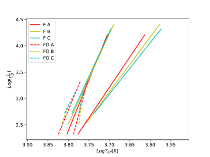
Figure 1: F and FO instability strips at fixed mixing length parameter $\alpha=1.5$ for the assumed A, B, C ML relations.

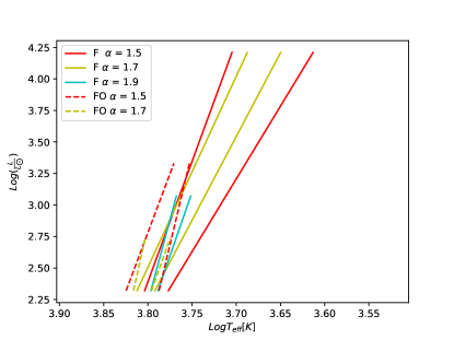
Figure 2: Canonical F and FO instability strips for the various assumption about superadiabatic convective efficiency.

3.3 The light and radial velocity curves

In this subsection, we present the new theoretical atlas of light and radial velocity curves for both F and FO modes, resulting from the nonlinear computation of full amplitude models. The predicted bolometric light curves (left panels) and radial velocity variations (right panels) are shown in Figure 3 for the canonical model sequences. The curves are plotted over two consecutive pulsation cycles, as a function of the pulsation phase. In each plot, dashed lines refer to FO models, whereas solid lines represent F models. In the left panel, on each light curve the period in days of the model is labeled while in the right panel, on each radial velocity curve the static effective temperature in kelvin is labeled. The decrease of the amplitudes of both light and radial velocity curves is an expected result related to the quenching effect of convection on pulsation. As $\alpha$ increases the efficiency of superadiabtic convection increases, making the driving mechanisms of pulsation less and less efficient and the amplitude of the oscillation smaller and smaller. Moreover, positive values of radial velocity along the curves indicate an expansion phase for the stellar envelope, while negative values of the velocity correspond to a contraction phase. The complete atlas of the bolometric light curves for the various assumptions about the ML relation and the superadiabatic convection efficiency are available in the Appendix.

Focusing on canonical models (luminosity level A) with $\alpha=1.5$, we notice that for masses lower or equal than 5 $M_{\odot}$ the curve amplitudes steadily decrease as the effective temperature decreases, moving from the FBE to the FRE. Above $\sim$ $5M_{\odot}$ this trend is less evident because the FO pulsation is no more efficient. In particular in the period range from $\sim 7$ to $\sim 12$ days a secondary maximum (bump) is present in the light and radial velocity curves. For this reason, Cepheids in this period range are called ”bump Cepheids”. The evolution of the bump pulsation phase from the descending to the ascending branch of the curve is the so called Hertzprung progression (HP) (Bono et al., 2000c). At the center of the HP the principal and secondary maximum are very close in magnitude and the pulsation amplitude often reaches a minimum. A detailed investigation of the dependence of the period corresponding to the HP center on metallicity is postponed to a future paper.

$M/M_{\odot}\,$=3.0    log ($L/L_{\odot})\,$=2.32    $\alpha=1.5$

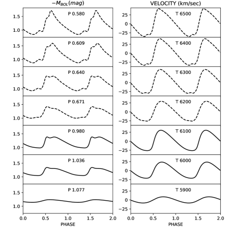
Figure 3: Bolometric light curves (left panel) and radial velocity curves (right panel) for a sequence of non linear F (solid line) and FO models (dashed lines) derived at fixed mass, luminosity, $\alpha$ parameter (see labeled values on the top of the plot) adopting the canonical ML relation.

$M/M_{\odot}\,$=4.0    log ($L/L_{\odot})\,$=2.74    $\alpha=1.5$

FIG.3-Continued.

$M/M_{\odot}\,$=5.0    log ($L/L_{\odot})\,$=3.07    $\alpha=1.5$

FIG.3-Continued.

$M/M_{\odot}\,$=6.0    log ($L/L_{\odot})\,$=3.33    $\alpha=1.5$

FIG.3-Continued.

$M/M_{\odot}\,$=7.0    log ($L/L_{\odot})\,$=3.56    $\alpha=1.5$

FIG.3-Continued.

$M/M_{\odot}\,$=8.0    log ($L/L_{\odot})\,$=3.75    $\alpha=1.5$

FIG.3-Continued.

$M/M_{\odot}\,$=9.0    log ($L/L_{\odot})\,$=3.92    $\alpha=1.5$

FIG.3-Continued.

$M/M_{\odot}\,$=10.0    log ($L/L_{\odot})\,$=4.08    $\alpha=1.5$

FIG.3-Continued.

$M/M_{\odot}\,$=11.0    log ($L/L_{\odot})\,$=4.21    $\alpha=1.5$

FIG.3-Continued.

3.3.1 The effect of the assumed Mass-Luminosity relation

To show the effect of a variation of the ML relation on the predicted light and radial velocity curves,we chose two models whose trend is representative of all other models.
In the panels (a) e (b) of Figure (4) we show the light and radial velocity curves of a F model respectively, at fixed $\frac{M}{M_{\odot}}=9.0$, $T_{eff}=4600K$ and $\alpha=1.5$ but for three different levels of luminosity (case A, B and C). As in Figure (4), the panels (a) and (b) in Figure (5) show the similar comparison for a FO model with $\frac{M}{M_{\odot}}=3.0$, $T_{eff}=6300K$ and $\alpha=1.5$. These plots confirm that both the morphology and amplitude of light and radial velocity curves depend on the assumed ML relation.

Moreover, inspection of B and C model sets indicates that in these cases longer periods are found at fixed mass due to the increased luminosity levels. As a consequence, ”bump Cepheids” are found at lower masses and the center of the HP is found at slightly shorter periods. This trend, once the metallicity is known, makes the HP phenomenon a useful tracer of Cepheid ML relation.

3.3.2 The effect of the assumed superadiabatic convective efficiency

As discussed above, the main effect of superadiabatic convection is to quench pulsation so that lower pulsation amplitudes are expected as $\alpha$ increases from 1.5 to 1.7 and 1.9. Assuming a canonical ML, Figure 6 and Figure 7 show the comparison between the light and radial velocity curves obtained for the three values of $\alpha$ but at fixed stellar parameters correspond to a F and a FO model with $\frac{M}{M_{\odot}}=4.0$, $T_{eff}=5900K$ and and $\frac{M}{M_{\odot}}=4.0$, $T_{eff}=6200K$, respectively. The morphology of the curves gets smoother and the pulsation amplitude decreases as $\alpha$ increases. In particular the FO pulsation disappears for $\alpha=1.9$ because at this value of $\alpha$ the quenching effect is very efficient and the pulsation disappears. The same trend is followed by all other models.

3.4 The Period-Radius and the Period-Mass-Radius relations

An important aspect of Cepheid research concerns the use of CC to infer stellar radii. CC are known to obey to both PR and PMR relations, the former involving an averaging operation over the finite width in effective temperature of the instability strip (Bono et al., 2001). The PR relations are used to derive the stellar radii directly from the pulsation periods, whereas PMR relations can be used to infer an independent value of the stellar mass, once known the period and the radius, to be compared with evolutionary mass estimates. The coefficients of the PR and PMR relations derived from current nonlinear model sets are reported in Tables LABEL:pr_f_fo and LABEL:pmr_f_fo for the F and FO models, respectively. Figure 8 shows the PR relations assuming the canonical ML relation for the three values of $\alpha$ for F and FO models and Figure 9 shows the PR relations at fixed $\alpha=1.5$ for ML relation from case A to B and C for F models. We confirm previous results by Bono et al. (1998) that the PR relation does not vary considerably with the different assumptions of the ML relation (see Table LABEL:pr_f_fo). Moreover varying the efficiency of superadiabatic convection has a mild effect on the PR coefficients.

Furthermore, we perform a comparison with literature relations of our PR (Figure 9). We confirm a general good agreement with Molinaro et al. (2012) and Gallenne et al. (2017) PR relations. However we better reproduce Molinaro et al. (2012) relation at shorter periods whereas the opposite occurs with Gallenne et al. (2017) relation. We finally note that the PR relations obtained by Molinaro et al. (2012) and Gallenne et al. (2017) depend on the assumed projection-factor (p-factor) value, while those derived by the models do not depend on this parameter (Ragosta et al., 2019) . Therefore a comparison between these two independent derivations allows us to put constraints on the value of the p-factor (e.g.Natale et al. (2008); Marconi et al. (2013b)) that plays a key role in the study of pulsating stars. Even if the investigation of the p-factor and of its dependence on the pulsation period is beyond the scope of the present paper, from the combination of our extended atlas of pulsation models with the large sample of radial velocity curves that will be provided by the Gaia mission, we will be able to constrain the p-factor with a much more robust statistics than in previous studies.

Figure 4: Light (a) and radial velocity (b) curves of $T_{eff}=4600K$, $M/M_{\odot}\,$=9.0, $\alpha=1.5$ F model for three levels of luminosity.

Figure 5: Light (a) and radial velocity (b) curves of $T_{eff}=6300K$, $M/M_{\odot}\,$=3.0, $\alpha=1.5$ FO model for different levels of luminosity.

Figure 6: Light (a) and radial velocity (b) curves for $M/M_{\odot}\,$=4.0, $T_{eff}=5900K$ F model for the canonical ML assumption.

Figure 7: Light (a) and radial velocity (b) curves for $M/M_{\odot}\,$=4.0, $T_{eff}=6200K$ FO model for the canonical ML assumption.

Table 7: PR coefficients ($\log R=a+b\log P$) for F and FO Galactic Cepheids derived by adopting A, B , C ML relations.

$\alpha$	ML	a	b	$\sigma_{a}$	$\sigma_{b}$	$R^{2}$
F
1.5	A	1.142	0.702	0.004	0.003	0.998
1.5	B	1.128	0.685	0.005	0.003	0.998
1.5	C	1.104	0.680	0.005	0.003	0.998
1.7	A	1.140	0.705	0.004	0.003	0.999
1.7	B	1.126	0.685	0.005	0.003	0.999
1.7	C	1.105	0.678	0.005	0.003	0.999
1.9	A	1.124	0.743	0.003	0.007	0.999
1.9	B	1.101	0.729	0.003	0.008	0.999
1.9	C	1.077	0.715	0.003	0.005	0.999
FO
1.5	A	1.242	0.768	0.001	0.005	0.999
1.5	B	1.216	0.762	0.003	0.015	0.997
1.5	C	1.193	0.742	0.003	0.009	0.997
1.7	A	1.243	0.773	0.002	0.009	0.840

Table 7: continued.

Table 8: PMR coefficients ($\log R=a+b\log P+c\log M$) for F and FO Galactic Cepheids derived by adopting A, B , C ML relations.

$\alpha$	ML	a	b	c	$\sigma_{a}$	$\sigma_{b}$	$\sigma_{c}$	$R^{2}$
F
1.5	A	-1.641	-0.890	1.830	0.007	0.06	0.03	0.999
1.5	B	-1.709	-0.920	1.874	0.01	0.072	0.03	0.998
1.5	C	-1.721	-0.687	1.784	0.01	0.06	0.03	0.998
1.7	A	-1.642	-1.144	1.948	0.008	0.14	0.06	0.999
1.7	B	-1.725	-1.194	2.001	0.01	0.13	0.06	0.999
1.7	C	-1.687	-0.583	1.728	0.02	0.11	0.05	0.999
1.9	A	-1.570	-0.778	1.737	0.02	0.3	0.1	0.999
1.9	B	-1.573	-0.720	1.709	0.01	0.09	0.05	0.999
1.9	C	-1.587	-0.547	1.654	0.01	0.06	0.03	0.999
FO
1.5	A	-1.659	-0.564	1.590	0.005	0.06	0.03	0.999
1.5	B	-1.695	-0.779	1.707	0.02	0.1007	0.05	0.999
1.5	C	-1.738	-0.698	1.704	0.01	0.06	0.03	0.999
1.7	A	-1.644	-0.589	1.591	0.01	0.1	0.05	0.902

Table 8: continued.

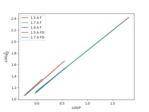
Figure 8: PR relations for F and FO Galactic Cepheids derived by adopting canonical ML relation and $\alpha=1.5$, $\alpha=1.7$, $\alpha=1.9$.

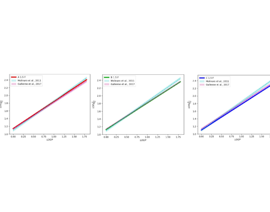
Figure 9: PR relations for F Galactic Cepheids derived by adopting $\alpha=1.5$ and A, B , C ML relations compared with similar results available in literature.

4 Predicted light curves, mean magnitudes and colors in the Gaia photometric system

The bolometric light curves presented in Section 3 have been converted in the Gaia photometric system passbands, namely $G$, $G_{BP}$ and $G_{RP}$, using the ATLAS9 non-overshooting model atmospheres (Castelli & Kurucz, 2003). This provides the first theoretical catalogue of Gaia light curves. The predicted light curves for $\alpha=1.5$ and masses ranging from 3 to 11 $M_{\odot}$ are shown in Figure 10 where the green line indicate the $G_{BP}$ band, the blue line the $G$ band and the orange line the $G_{RP}$ band. Dashed and solid lines represent the FO and F models, respectively. On each light curve the effective temperature in kelvin and the period in days of the model is labeled. The complete atlas of the light curves in the Gaia photometric system for the various assumptions about the ML relation and the superadiabatic convection efficiency are available in the Appendix. We note that the morphology of the predicted Gaia light curves follow the features of the bolometric ones. The converted light curves allow us to derive intensity-averaged mean magnitudes and colors in the Gaia filters, namely magnitudes $<M_{G}>$, $<M_{G_{BP}}>$, $<M_{G_{RP}}>$ and color $<G_{BP}>$ - $<G_{RP}>$. The three mean magnitudes are reported in Tables LABEL:gaia_mean_f and LABEL:gaia_mean_fo for each F and FO model.

$M/M_{\odot}\,$=3.0    log ($L/L_{\odot})\,$=2.32    $\alpha=1.5$

Figure 10: Theoretical Gaia light curves for a sequence of non linear F (solid line) and FO models (dashed line) derived at fixed mass, luminosity, $\alpha$ parameter (see labeled values on the top of the plot) adopting the canonical ML relation.

$M/M_{\odot}\,$=4.0    log ($L/L_{\odot})\,$=2.74    $\alpha=1.5$

FIG.10-Continued.

$M/M_{\odot}\,$=5.0    log ($L/L_{\odot})\,$=3.07    $\alpha=1.5$

FIG.10-Continued.

$M/M_{\odot}\,$=6.0    log ($L/L_{\odot})\,$=3.33    $\alpha=1.5$

FIG.10-Continued.

$M/M_{\odot}\,$=7.0    log ($L/L_{\odot})\,$=3.56    $\alpha=1.5$

FIG.10-Continued.

$M/M_{\odot}\,$=8.0    log ($L/L_{\odot})\,$=3.75    $\alpha=1.5$

FIG.10-Continued.

$M/M_{\odot}\,$=9.0    log ($L/L_{\odot})\,$=3.92    $\alpha=1.5$

FIG.10-Continued.

$M/M_{\odot}\,$=10.0    log ($L/L_{\odot})\,$=4.08    $\alpha=1.5$

FIG.10-Continued.

$M/M_{\odot}\,$=11.0    log ($L/L_{\odot})\,$=4.21    $\alpha=1.5$

FIG.10-Continued.

Stellar mass (solar units).

Logarithmic luminosity (solar units).

Effective temperature(K).

Mixing length parameter.

Mass-Luminosity relation.

Gaia passband G.

Gaia passband $G_{BP}$.

Gaia passband $G_{RP}$.

Table 9: Mean magnitudes in the Gaia filters for F models at varying the ML relation and the $\alpha$ pareameter. Full tables are available in the Appendix.

			Z=0.02	Y= 0.28
Ma	logLb	$T_{eff}$c	$\alpha$d	MLe	Gf	$G_{BP}$g	$G_{RP}$h
(1)	(2)	(3)	(4)	(5)	(6)	(7)	(8)
3.0	2.32	5900	1.5	A	1.31	-1.03	-1.75
3.0	2.32	6000	1.5	A	1.31	-1.05	-1.73
…
4.0	2.74	5500	1.5	A	2.34	-1.99	-2.85
4.0	2.74	5600	1.5	A	2.34	-2.01	-2.83
…
5.0	3.07	5300	1.5	A	3.13	-2.74	-3.68
5.0	3.07	5400	1.5	A	3.14	-2.77	-3.67
…
6.0	3.33	5000	1.5	A	3.75	-3.30	-4.36
6.0	3.33	5100	1.5	A	3.76	-3.33	-4.36
…
7.0	3.56	4800	1.5	A	4.26	-3.77	-4.91
7.0	3.56	4900	1.5	A	4.28	-3.81	-4.90
…
8.0	3.75	4600	1.5	A	4.70	-4.16	-5.39
8.0	3.75	4700	1.5	A	4.72	-4.21	-5.39
…
9.0	3.92	4400	1.5	A	5.07	-4.48	-5.79
9.0	3.92	4500	1.5	A	5.09	-4.53	-5.80
…
10.0	4.08	4200	1.5	A	5.38	-4.75	-6.15
10.0	4.08	4300	1.5	A	5.41	-4.80	-6.16
…
11.0	4.21	4100	1.5	A	5.68	-5.02	-6.47
11.0	4.21	4200	1.5	A	5.72	-5.08	-6.49
…

Table 9: continued.

Stellar mass (solar units).

Logarithmic luminosity (solar units).

Effective temperature(K).

Mixing length parameter.

Mass-Luminosity relation.

Gaia passband G.

Gaia passband $G_{BP}$.

Gaia passband $G_{RP}$.

Table 10: The same as in Table LABEL:gaia_mean_f but for FO models.

			Z=0.02	Y= 0.28
Ma	logLb	$T_{eff}$c	$\alpha$d	MLe	Gf	$G_{BP}$g	$G_{RP}$h
(1)	(2)	(3)	(4)	(5)	(6)	(7)	(8)
3.0	2.32	6200	1.5	A	-1.32	-1.08	-1.70
3.0	2.32	6300	1.5	A	-1.32	-1.10	-1.68
…
4.0	2.74	5900	1.5	A	-2.36	-2.08	-2.80
4.0	2.74	6000	1.5	A	-2.37	-2.10	-2.78
…
5.0	3.07	5800	1.5	A	-3.17	-2.88	-3.63
5.0	3.07	5900	1.5	A	-3.18	-2.90	-3.61
…
6.0	3.33	5800	1.5	A	-3.84	-3.54	-4.29

Table 10: continued.

4.1 The Period-Luminosity-Color and the Period-Wesenheit relations in the Gaia filters

The mean magnitudes and colors derived in the previous section can be used to derive the first theoretical PLC and PW relations in the Gaia filters. The coefficients of these relations at varying the ML relation and the efficiency of the superadiabatic convection, are reported in Table LABEL:plc_f_fo and Table LABEL:w_f_fo for F and FO models, respectively. To derive the Wesenheit magnitude we adopt the relation provided by Ripepi et al. (2019) $<W>=<G>-1.9<G_{BP}-G_{RP}>$. Both the PLC and the PW relations hold for each individual pulsator thus allowing us to derive individual distances of observed Cepheids in the Gaia database. We notice that the PLC and PW relations, and in turn the individual distances derived by applying them to the observed pulsators, depend on the assumed ML relation but are almost insensitive to the value of the mixing length parameter. In particular assuming $\alpha=1.5$, if we consider a F mode Cepheid pulsator with $P=10$ days and $<G_{BP}>$ - $<G_{RP}>$ = 1.0 mag, the $<G>$ magnitude obtained from the theoretical PLC relation varies from $<G>$= $-4.11$ mag at the canonical ML (case A) to $<G>$= $-3.94$ mag for a ML brighter by 0.2 dex (case B) and to $<G>$ = $-3.79$ mag for a ML brighter by 0.4 dex (case C). Consequently assuming $P=10$ days and $<G_{BP}>$ - $<G_{RP}>$ = 1.0 mag, the difference in the predicted $<G>$ magnitude amounts to $0.1$ mag and $0.3$ mag when the ML relation changes from case A to B and C, respectively and assuming the canonical case A, the $<G>$ magnitude obtained from the PLC relation can change up to 0.1 mag when moving from $\alpha=1.5$ to $\alpha=1.9$. In order to better exemplify what could occur in typical extragalactic distance scale applications, we performed the same kind of test with F mode PLC relations at fixed periods of 30 and 100 days and $<G_{BP}>$ - $<G_{RP}>$ = 1.0 mag. As a result, we found that, assuming $\alpha=1.5$ and $P=30$ days, $<G>$ varies from $-5.91$ (case A) to $-5.73$ (case B) and $-5.57$ case (C), whereas for a still longer period (P=100 days) $<G>$ varies from $-7.89$ (case A) to $-7.7$ (case B) and $-7.51$ (case C). On this basis we conclude that the effects related to superadiabatic convection on the predicted $<G>$ magnitude amount to about 0.15 mag and 0.20 mag for $P=30$ days and $P=100$ days respectively, whereas the effects related to variations in the ML relation can be as large as 0.4 mag, for the two period assumptions. Similar considerations hold for the predicted F mode PW relations. As for FO pulsators, both PLC and PW relations are insensitive to variations in the efficiency of superadiabatic convection.”

Table 11: PLC coefficients ($<G>$=a+b$\log P$ +c($<G_{BP}>$ - $<G_{RP}>$) for F and FO Galactic Cepheids derived by adopting A, B , C ML relations and $\alpha=1.5$, $\alpha=1.7$ and $\alpha=1.9$ in the Gaia filters.

$\alpha$	ML	a	b	c	$\sigma_{a}$	$\sigma_{b}$	$\sigma_{c}$	$R^{2}$
F
1.5	A	-3.52	-3.78	3.19	0.04	0.03	0.06	0.998
1.5	B	-3.45	-3.76	3.27	0.03	0.03	0.06	0.998
1.5	C	-3.27	-3.71	3.18	0.03	0.02	0.05	0.998
1.7	A	-3.61	-3.94	3.42	0.09	0.06	0.15	0.999
1.7	B	-3.65	-3.91	3.62	0.08	0.06	0.14	0.998
1.7	C	-3.21	-3.69	3.09	0.06	0.04	0.11	0.998
1.9	A	-3.33	-3.92	3.05	0.12	0.05	0.19	0.999
1.9	B	-3.24	-3.93	3.14	0.07	0.01	0.12	0.999
1.9	C	-2.89	-3.81	2.81	0.03	0.02	0.06	0.999
FO
1.5	A	-3.53	-3.95	2.48	0.04	0.02	0.06	0.999
1.5	B	-3.49	-3.96	2.63	0.06	0.04	0.11	0.999
1.5	C	-3.45	-3.97	2.80	0.08	0.07	0.16	0.999
1.7	A	-3.49	-3.90	2.38	0.06	0.03	0.11	0.999

Table 11: continued.

Table 12: PW coefficients ($<W>=<G>-1.9<G_{BP}-G_{RP}>=a+b\log P$) for F and FO Galactic Cepheids derived by adopting A, B , C ML relations and , $\alpha=1.5$, $\alpha=1.7$ and $\alpha=1.9$ in the Gaia filters.

$\alpha$	ML	a	b	$\sigma_{a}$	$\sigma_{b}$	$R^{2}$
F
1.5	A	-2.73	-3.26	0.04	0.03	0.995
1.5	B	-2.68	-3.18	0.05	0.03	0.994
1.5	C	-2.56	-3.16	0.07	0.05	0.992
1.7	A	-2.75	-3.37	0.06	0.05	0.998
1.7	B	-2.68	-3.20	0.03	0.04	0.996
1.7	C	-2.54	-3.23	0.08	0.06	0.997
1.9	A	-2.64	-3.52	0.05	0.11	0.999
1.9	B	-2.55	-3.44	0.09	0.21	0.999
1.9	C	-2.51	-3.11	0.08	0.11	0.999
FO
1.5	A	-3.17	-3.80	0.02	0.07	0.999
1.5	B	-3.02	-3.85	0.02	0.13	0.996
1.7	A	-3.24	-3.96	0.05	0.28	0.999

Table 12: continued.

5 Theoretical versus Gaia Data Release 2 parallaxes

In this section we perform a comparison between the individual theoretical parallaxes based on the PW relations in the Gaia filters and the observed Classical F and FO Cepheids parallaxes taken from the recent catalog made by Ripepi et al. (2019). In their work Ripepi and collaborators reclassify the DR2 Galactic Cepheids and provide accurate PL and PW relations in the Gaia passbands. To ensure a good astrometry we chose from the sample the Classical F and FO Cepheids for which the magnitude in G is brighter than 6 mag and the renormalized unit weight error values (RUWE) defined by Lindegren (2018) is less than 1.4.

The theoretical PW relations derived in the previous subsection are applied to the observed periods and Gaia magnitudes and colors reported in the quoted catalog to derive reddening-free individual distances and in turn theoretical estimates of individual parallaxes. The latter can be directly compared with Gaia DR2 results as shown in Figure 11. These plots show the difference between predicted and Gaia DR2 parallaxes versus Gaia DR2 parallaxes for the labeled assumptions concerning the ML relation and the $\alpha$ parameter. In each panel, the obtained mean offset (solid line) is compared with the mean offset derived by Riess et al. (2018) (dashed line) and corresponding to $<\Delta\varpi>$= 0.046$\pm$ 0.013 mas, as derived from the HST space astrometric technique. We notice that this value is reproduced within the errors by our models apart from a few cases at the brightest luminosity levels (F mode case C). We also note that variations in the parallax of the order of $\pm 0.02$ mas at a typical parallax of the order of 0.5 mas implies a relative parallax error and in turn a relative distance error of 4$\%$. This also reflects on the estimated $H_{0}$: smaller parallaxes by 4$\%$ implies longer distances and in turn smaller values of $H_{0}$ by 4$\%$ that would be enough to significantly reduce, if not remove the tension.

6 Conclusions

In the context of a theoretical project aimed to investigate the residual systematic effects on the Cepheid-based extragalactic distance scale, a new extended set of nonlinear convective models of Classical Cepheids at solar chemical composition and a wide range of stellar masses and luminosity levels has been computed. All the predicted pulsation observables for the F and FO models and their dependence on the ML relation and the efficiency of superadiabatic convection have been discussed. The main results are the following:

1. As expected, the predicted instability strip gets narrower as the efficiency of superadiabatic convection increases, whereas it does not significantly depend on the assumed ML relation apart from the brighter luminosity levels.

2. Analytical relations connecting the pulsation period of the F and FO models to the intrinsic stellar properties, M, L and $T_{eff}$, have been derived for each assumed mixing length parameter, showing a mild dependence on this value.

3. From the predicted radius curves, mean radii and in turn theoretical PR and PMR relations have been derived. PR relations have been compared with similar relations in the literature, showing a good agreement. Moreover, we confirm the results by Bono et al. (1998) for which the PR and PMR relations do not vary considerably with the different assumptions of the ML relation.

4. The obtained bolometric light curves are sensitive to the value of the mixing length parameter with the amplitude decreasing as the efficiency of superadiabatic convection increases, whereas the dependence on the ML relation is much less important.

5. From this set of models the first atlas of theoretical light curves of F and FO Galactic Cepheids converted in the Gaia filters is provided and it shall be made available to the scientific community.

6. The obtained mean magnitudes and colors are used to derive the first theoretical Cepheid PLC and PW relations in the Gaia filters.

Finally the above derived relations have been applied to Galactic Cepheids data in the Gaia DR2 database to derive theoretical individual parallaxes which have been compared with the Gaia DR2 ones. In particular, we find that the mean offset derived by Riess et al. (2018) and corresponding to $<\Delta\varpi>$= 0.046$\pm$0.013 mas, is reproduced within the errors by our models apart from a few cases at the brightest luminosity levels (F mode case C). To quantify such an offset and its dependence on the physical and numerical assumptions is crucial to understand and try to reduce the Hubble constant tension. In particular, a variation in the parallax of the order of $\pm 0.02$ mas at a typical parallax of the order of 0.5 mas implies a relative parallax error and in turn a relative error on $H_{0}$ of 4$\%$.

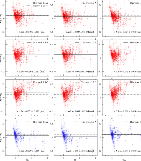
Figure 11: Parallax difference $\varpi_{T}$ - $\varpi_{G}$ for F (red points) and FO (blue points) Galactic Cepheids as a function of Gaia DR2 parallax $\varpi_{G}$.

References

- Bono et al. (2000a) Bono, G., Caputo, F., Cassisi, S., et al. 2000a, ApJ, 543, 955, doi: 10.1086/317156
- Bono et al. (1998) Bono, G., Caputo, F., & Marconi, M. 1998, ApJ, 497, L43, doi: 10.1086/311270
- Bono et al. (2000b) Bono, G., Castellani, V., & Marconi, M. 2000b, ApJ, 529, 293, doi: 10.1086/308263
- Bono et al. (2001) Bono, G., Gieren, W. P., Marconi, M., & Fouqué, P. 2001, ApJ, 552, L141, doi: 10.1086/320344
- Bono et al. (1999) Bono, G., Marconi, M., & Stellingwerf, R. F. 1999, ApJS, 122, 167, doi: 10.1086/313207
- Bono et al. (2000c) —. 2000c, A&A, 360, 245. https://arxiv.org/abs/astro-ph/0006229
- Carini et al. (2014) Carini, R., Brocato, E., Marconi, M., & Raimondo, G. 2014, A&A, 561, A110, doi: 10.1051/0004-6361/201322802
- Castelli & Kurucz (2003) Castelli, F., & Kurucz, R. L. 2003, in IAU Symposium, Vol. 210, Modelling of Stellar Atmospheres, ed. N. Piskunov, W. W. Weiss, & D. F. Gray, A20. https://arxiv.org/abs/astro-ph/0405087
- Clementini et al. (2019) Clementini, G., Ripepi, V., Molinaro, R., et al. 2019, A&A, 622, A60, doi: 10.1051/0004-6361/201833374
- Di Criscienzo et al. (2004) Di Criscienzo, M., Marconi, M., & Caputo, F. 2004, Mem. Soc. Astron. Italiana, 75, 190
- Fiorentino et al. (2007) Fiorentino, G., Marconi, M., Musella, I., & Caputo, F. 2007, A&A, 476, 863, doi: 10.1051/0004-6361:20077587
- Freedman et al. (2001) Freedman, W. L., Madore, B. F., Gibson, B. K., et al. 2001, ApJ, 553, 47, doi: 10.1086/320638
- Gaia Collaboration et al. (2016) Gaia Collaboration, Prusti, T., de Bruijne, J. H. J., et al. 2016, A&A, 595, A1, doi: 10.1051/0004-6361/201629272
- Gaia Collaboration et al. (2018) Gaia Collaboration, Brown, A. G. A., Vallenari, A., et al. 2018, A&A, 616, A1, doi: 10.1051/0004-6361/201833051
- Gallenne et al. (2017) Gallenne, A., Kervella, P., Mérand, A., et al. 2017, A&A, 608, A18, doi: 10.1051/0004-6361/201731589
- Holl et al. (2018) Holl, B., Audard, M., Nienartowicz, K., et al. 2018, A&A, 618, A30, doi: 10.1051/0004-6361/201832892
- Lindegren (2018) Lindegren, L. 2018, A&A
- Macri et al. (2006) Macri, L. M., Stanek, K. Z., Bersier, D., Greenhill, L. J., & Reid, M. J. 2006, ApJ, 652, 1133, doi: 10.1086/508530
- Marconi (2017) Marconi, M. 2017, in European Physical Journal Web of Conferences, Vol. 152, 06001, doi: 10.1051/epjconf/201715206001
- Marconi et al. (2005) Marconi, M., Musella, I., & Fiorentino, G. 2005, ApJ, 632, 590, doi: 10.1086/432790
- Marconi et al. (2010) Marconi, M., Musella, I., Fiorentino, G., et al. 2010, ApJ, 713, 615, doi: 10.1088/0004-637X/713/1/615
- Marconi et al. (2013a) Marconi, M., Molinaro, R., Bono, G., et al. 2013a, ApJ, 768, L6, doi: 10.1088/2041-8205/768/1/L6
- Marconi et al. (2013b) —. 2013b, ApJ, 768, L6, doi: 10.1088/2041-8205/768/1/L6
- Molinaro et al. (2012) Molinaro, R., Ripepi, V., Marconi, M., et al. 2012, Memorie della Societa Astronomica Italiana Supplementi, 19, 205
- Natale et al. (2008) Natale, G., Marconi, M., & Bono, G. 2008, ApJ, 674, L93, doi: 10.1086/526518
- Planck Collaboration et al. (2018) Planck Collaboration, Aghanim, N., Akrami, Y., et al. 2018, arXiv e-prints, arXiv:1807.06209. https://arxiv.org/abs/1807.06209
- Ragosta et al. (2019) Ragosta, F., Marconi, M., Molinaro, R., et al. 2019, MNRAS, 2480, doi: 10.1093/mnras/stz2881
- Riess et al. (2019) Riess, A. G., Casertano, S., Yuan, W., Macri, L. M., & Scolnic, D. 2019, ApJ, 876, 85, doi: 10.3847/1538-4357/ab1422
- Riess et al. (2011) Riess, A. G., Macri, L., Casertano, S., et al. 2011, ApJ, 730, 119, doi: 10.1088/0004-637X/730/2/119
- Riess et al. (2018) Riess, A. G., Casertano, S., Yuan, W., et al. 2018, ApJ, 861, 126, doi: 10.3847/1538-4357/aac82e
- Ripepi et al. (2019) Ripepi, V., Molinaro, R., Musella, I., et al. 2019, A&A, 625, A14, doi: 10.1051/0004-6361/201834506
- Romaniello et al. (2008) Romaniello, M., Primas, F., Mottini, M., et al. 2008, A&A, 488, 731, doi: 10.1051/0004-6361:20065661