Equilibrium models of the Milky Way mass are biased high by the LMC

Abstract

Recent measurements suggest that the Large Magellanic Cloud (LMC) may weigh as much as 25% of the Milky Way. In this work we explore how such a large satellite affects mass estimates of the Milky Way based on equilibrium modelling of the stellar halo or other tracers. In particular, we show that if the LMC is ignored, the Milky Way mass is overestimated by as much as 50%. This bias is due to the bulk motion in the outskirts of the Galaxy’s halo and can be, at least in part, accounted for with a simple modification to the equilibrium modelling. Finally, we show that the LMC has a substantial effect on the orbit Leo I which acts to increase its present day speed relative to the Milky Way. We estimate that accounting for a $1.5\times 10^{11}M_{\odot}$ LMC would lower the inferred Milky Way mass to $\sim 10^{12}M_{\odot}$.

1 Introduction

The Large Magellanic Cloud (LMC) is the brightest satellite of the Milky Way and has been known since antiquity (e.g. Al Sufi, 964). The first suggestion that the LMC could have a significant effect on our Galaxy was proposed by Kerr (1957) and Burke (1957) based on the observations of the deformed atomic hydrogen disk in the Milky Way. However, calculations in those works based on the mass of the LMC at the time showed that the LMC was unlikely to explain the deformation. Avner & King (1967) followed this up with a more general exploration of the effect of the LMC. Their discussion mostly focused on how the LMC could torque and twist the disk of the Milky Way assuming it was on a relatively circular orbit, although they also included a prescient discussion of whether or not the LMC was bound to the Small Magellanic Cloud (SMC) or to our Galaxy.

More recent work has shown that the Magellanic Clouds are likely bound to each other and are on their first approach to the Milky Way (Kallivayalil, van der Marel & Alcock, 2006; Besla et al., 2007; Kallivayalil et al., 2013). Alongside this, a number of works have shown that the LMC has a large total mass, $M_{\rm LMC}\sim 10^{11}-2.5\times 10^{11}M_{\odot}$, based on abundance matching (e.g. Moster, Naab & White, 2013), assuming the SMC was originally bound to the LMC (Kallivayalil et al., 2013), using the timing argument with Andromeda combined with the nearby Hubble flow (Peñarrubia et al., 2016), perturbations to the Milky Way disk (Laporte et al., 2018; Gardner, Hinkel & Yanny, 2020), quantifying the effect of the LMC on Orphan stream (Erkal et al., 2019), and modelling the satellites of the LMC (Erkal & Belokurov, 2019).

These high LMC masses can induce a substantial reflex motion in the Milky Way (Gómez et al., 2015) and fits to the Orphan stream predicted this could be as large as $\sim 50$ km/s (Erkal et al., 2019). This reflex motion should be most apparent beyond $\sim 30$ kpc where the orbital periods of stars are longer than the infall time of the LMC. Along these lines, Garavito-Camargo et al. (2019) studied the effect of the LMC on the stellar halo of the Milky Way and predicted that there should be an over-dense wake behind the LMC as well as substantial non-equilibrium motion in the outskirts of our Galaxy. Belokurov et al. (2019) showed that the Pisces over-density (Watkins et al., 2009) was consistent with this wake both in 3d shape and radial velocity. Petersen & Peñarrubia (2020) also simulated the infall of the LMC and found similar results. Thus, multiple lines of evidence suggest that the LMC has had a large effect on our Galaxy, making it significantly out of equilibrium.

In this work we will examine how the disequilibrium of our Galaxy affects our ability to measure its mass. In particular, we will use the mass estimator from Watkins, Evans & An (2010) which assumes that our Galaxy is in equilibrium. This estimator has been used in a number of recent works to measure the mass of our Galaxy out to radii where these non-equilibrium effects are significant (e.g. Sohn et al., 2018a; Watkins et al., 2019; Fritz et al., 2020). We will also explore how this reflex motion affects the mass estimate based on Leo I (Boylan-Kolchin et al., 2013). This paper is organized as follows. In Section 2 we will explore the effect of the LMC on our Galaxy and in particular how it biases the mass estimator. In Section 3 we search for the predicted reflex motion using satellites of the Milky Way, explore how this reflex motion affects the motion of Leo I, and conclude.

2 Effect of LMC on the Milky Way’s halo

In order to simulate the effect of the LMC on a tracer population around the Milky Way, we use a suite of simulations with a variety of LMC masses. The fiducial set of simulations are identical to those described in Belokurov et al. (2019). The simulations in that work are fast since the Milky Way and LMC are not resolved with full $N$-body dynamics. Instead, they are modelled as single particles sourcing their respective potentials. The Milky Way is modelled using the MWPotential2014 from Bovy (2015) where the bulge is replaced by an equal mass Hernquist Hernquist (1990) profile for speed. The LMC is modeled as a Hernquist profile. In this framework, the LMC is rewound from its present day position, the stellar halo is initialized as a population of tracer particles, and the system is evolved forward to the present. We assume that the Sun is located at a distance of 8.122 kpc from the Galactic center (Gravity Collaboration et al., 2018).

Figure 1 shows the effect of a $1.5\times 10^{11}M_{\odot}$ LMC on the stellar halo of the Milky Way. This demonstrates that this technique gives broadly similar answers to Garavito-Camargo et al. (2019) which studied the motions of both the LMC and Milky Way with $N$-body simulations. Comparing the two approaches it is clear that both the “local wake” (aligned with the LMC’s past orbit) and the “global wake” (mostly in the Northern hemisphere) are reproduced. This is due to the fact that the simulations in Belokurov et al. (2019) accounted for the direct effect of the LMC on the stellar halo, as well as the reflex motion of the Milky Way in response to the LMC. However, two key aspects missing from our simulations are the deformation of the Milky Way and LMC in response to each other and any resonances in the Milky Way’s halo. Given that Figure 1 closely resembles the results of Garavito-Camargo et al. (2019), these effects do not seem to be important for the bulk properties of the stellar halo.

One key result highlighted in Figure 1 is that the LMC induces a motion of the inner region of the Milky Way, within roughly 30 kpc, with respect to the outer part of the Galaxy. This streaming motion is mostly in the downwards (-$z$) direction. This is apparent in the third and fourth rows of Figure 1 which show that the distant stellar halo is moving upwards relative to the inner parts of the Galaxy. This effect was predicted in Erkal et al. (2019) which measured the mass of the LMC based on its effect on the Orphan stream. That work argued that the orbital timescales are short in the inner part of the Galaxy and thus these stars can respond adiabatically to the LMC, while stars in the outskirts of the Galaxy, where the orbital timescales are longer, do not respond coherently, thus giving rise to a bulk motion. Since the LMC’s past orbit has most recently been below the Milky Way, the Cloud can be seen as pulling the inner part of the Milky Way downwards. This effect was also seen in the simulations in Garavito-Camargo et al. (2019).

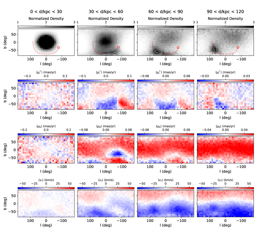
Figure 1: Effect of a $1.5\times 10^{11}M_{\odot}$ LMC on the Milky Way stellar halo in various distance bins. Each column shows a different range of distances (shown at the top of the plot). Top row shows the normalized stellar halo density. The red circle shows the present-day position of the LMC, the dashed-red curve shows the past orbit of the LMC, and the light blue curve shows the section of the LMC’s orbit in the given distance bin. There is a clear overdensity in the outer stellar halo which traces the past orbit of the LMC. Second row shows the mean reflex-corrected proper motion $\mu_{l}^{*}$. In the inner most distance slice, there is very little structure. However, in the more distant slices there are clear patterns in the proper motion related to the past orbit of the LMC. Third row shows the mean reflex-corrected proper motion $\mu_{b}$. Beyond 30 kpc, the mean proper motion is positive over most of the sky, showing that the stellar halo is moving upwards relative to the inner part of the Galaxy. Bottom row shows the mean reflex-corrected radial velocity. Beyond 30 kpc, there is a clear dipole with the halo in the Southern hemisphere having a negative radial velocity (i.e. approaching the Sun) and the halo in the Northern hemisphere having a positive radial velocity (i.e. receding from the Sun). This also shows that inner part of the Galaxy is moving downwards with respect to the outer part of the stellar halo. These results are qualitatively similar to the results in Garavito-Camargo et al. (2019).

This streaming motion suggests that equilibrium modelling will likely be biased in the presence of the LMC. To quantify this systematic error, we focus on the mass estimator from Watkins, Evans & An (2010) which makes use of the tracers 3d velocity. This has been used in several recent works (e.g. Sohn et al., 2018b; Watkins et al., 2019; Fritz et al., 2020) but due to the streaming motion relative to the outskirts of our Galaxy, we expect that any method which assumes dynamical equilibrium will be biased. This estimate is given by

$$M=\frac{\alpha+\gamma-2\beta}{3-2\beta}\frac{r_{\rm out}^{1-\alpha}}{G}\langle v^{2}r^{\alpha}\rangle,$$ (1)

where $\alpha$ is the power-law slope of the potential (i.e. $\psi(r)\propto r^{-\alpha}$), $\beta$ is the anisotropy of the tracer population, $\gamma$ is the power-law slope of the tracer density (i.e. $\rho\propto r^{-\gamma}$), $r$ is the galactocentric distance to each tracer, $v^{2}$ is the 3d speed of each tracer relative to the Galaxy, and $r_{\rm out}$ is the radius of the outermost tracer.

We apply this mass estimator to the simulated stellar haloes from Belokurov et al. (2019). In particular, we use the $5\times 10^{10}M_{\odot}$, $1.5\times 10^{11}M_{\odot}$, $2.5\times 10^{11}M_{\odot}$ LMC runs and the run with no LMC. First, as a reference, we use Equation 1 to measure the MW mass in the simulation without the LMC. For this stellar halo, we expect that the estimator in (1) will recover the true mass profile. We break the stellar halo into radial bins from 30 kpc to 200 kpc. For each bin, we use a bin width which is $\sim$19% of the radius so that the mass estimate is as accurate as possible. This results in 10 bins in the range 30-200 kpc. If we use significantly larger bins, then the power-law slope of the potential and tracer density can change significantly within each bin, making the estimator less precise. The results are shown in Figure 2. The green circles show the mass estimator applied to the simulation with no LMC. As expected, this faithfully reproduces the true mass distribution of the simulated Milky Way.

Next we consider the simulations with three different LMC masses. The resulting mass profiles are also shown in Figure 2 using different color symbols. As the LMC mass is increased, the Milky Way mass is progressively overestimated. Indeed, at 200 kpc, this can result in an up to $\sim$ 50% overestimate of the Milky Way mass. Interestingly, all of the measurements converge to the true Milky Way mass within $\sim 30$ kpc since within this region there is no significant bulk motion and the Milky Way is effectively in equilibrium.

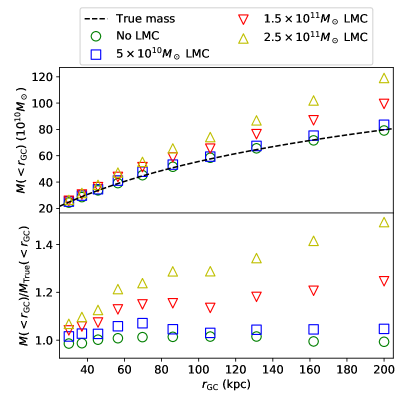
Figure 2: Mass estimator applied to simulated Milky Way in the presence of the LMC. Top panel shows the mass estimator applied to four simulations with various LMC masses. The simulation with no LMC matches the true mass quite well while as the LMC mass is increased, the inferred mass is increasingly biased. As expected, the estimates converge to the true value within $\sim$ 30 kpc since the Milky Way does not have any bulk motion within this region. Bottom panel shows the inferred mass divided by the true mass, i.e. the size of the bias. For the most massive LMC considered here, $2.5\times 10^{11}M_{\odot}$, the inferred mass is $\sim$ 50% higher than the true mass at 200 kpc. However, even at more modest radii of $\sim$ 50 kpc, this bias can reach 20%.

In Figure 3 we explore the bulk velocity induced by the LMC’s in-fall by computing the tracer mean velocity in radial shells. If the LMC is not included, the mean velocity is close to zero as expected since the stellar halo is in equilibrium. However, as the LMC mass is increased, the mean velocity grows significantly in the outer parts of the halo ($r>\sim 30$ kpc). The bulk motion of the distant stellar halo is mostly in the upwards (i.e. $+z$ direction). This is due to the fact that in the recent past, the LMC’s orbit has taken it below the plane of the Milky Way. As the Cloud passes its peri-centre, the short orbital timescales in the inner part of the Milky Way allow it to respond coherently, while the timescales in the outer part are too long. Thus, the inner part of the Milky Way is accelerated downwards relative to the outer parts as argued in Erkal et al. (2019).

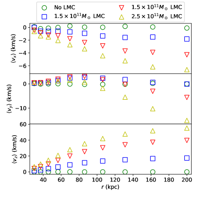
Figure 3: Magnitude of mean velocity in radial shells in the presence of various mass LMCs. If the LMC is not included, the mean velocity in all shells is close to zero, as expected if the system is in equilibrium. However, as the LMC mass is increased, the mean velocity beyond $\sim 30$ kpc increases to nearly $60$ km/s in the case of the $2.5\times 10^{11}M_{\odot}$ LMC. The velocity is mainly in the $+z$ direction (i.e. upwards): over the radial range considered here, the velocity is always within $\sim 18^{\circ}$ of the $+z$ direction. This large bulk velocity shows that the outer parts of the stellar halo are significantly out of equilibrium due to the LMC. Note that the y-range of each panel is different.

The simulations in Belokurov et al. (2019) were tailored to be similar to the stellar halo since they have an anisotropy of $\sim 0.5$ in agreement with recent measurements in the Galaxy (see e.g. Lancaster et al., 2019). In order to study how other tracer populations, i.e. globular clusters or dwarf galaxies, are affected we run two additional simulations. For these we have an anisotropy of $\sim 0$ and $\sim$ -$0.5$ to investigate how changing the anisotropy affects our results. As in Belokurov et al. (2019), the initial conditions are generated using agama (Vasiliev, 2019a) with the DoublePowerLaw distribution functions from Posti et al. (2015). For an anisotropy of $\sim$ 0, we use norm=1.5e10, j0=500, slopeIn=0, slopeOut=3.5, coefJrOut=1.175, coefJzOut=0.9125, jcutoff=1e5, cutoffStrength=2 and for an anisotropy of $\sim$ -$0.5$, we use norm=1.5e10, j0=500, slopeIn=0, slopeOut=3.5, coefJrOut=1.48, coefJzOut=0.76, jcutoff=1e5, cutoffStrength=2. For these different anisotropies, we only consider an LMC mass of $1.5\times 10^{11}M_{\odot}$. In Figure 4 we compare the mass estimator with three different anisotropy values and see that the estimator is similarly biased, independent of the anisotropy chosen. Thus, we should expect that estimates of the Milky Way with any tracer will be strongly affected.

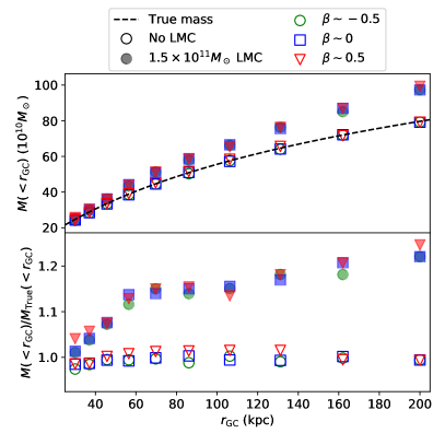
Figure 4: Mass estimator applied to stellar haloes with various anisotropies in the presence of the LMC. Top panel shows the mass estimator compared to the true mass and the bottom panel shows the mass estimator divided by the true mass. Since the anisotropy does not significantly affect the mass estimate, the bias induced by the LMC should be present in all tracer populations.

Since a lot of the velocity structure in Figure 1 appears to be due to the inner part of the Galaxy moving downwards with respect to the outer parts, we propose a slightly modified version of the estimator from Watkins, Evans & An (2010) which uses the velocity dispersion relative to the mean velocity:

$$M_{\bar{v}}=\frac{\alpha+\gamma-2\beta}{3-2\beta}\frac{r_{\rm out}^{1-\alpha}}{G}\langle(\mathbf{v}-\bar{\mathbf{v}})^{2}r^{\alpha}\rangle.$$ (2)

A comparison of this estimator versus the one in Equation 1 is shown in Figure 5 for eight different octants (marked according to their positive or negative position along each of $X,Y,Z$ axes). Two of the best octants are $(-,-,+)$ and $(+,-,+)$. These correspond to $l<0^{\circ}$ and $b>0^{\circ}$. Referring back to Figure 1, this is reassuringly the quadrant of the sky with the least structure in the velocity.

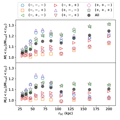
Figure 5: Mass estimator applied on different octants in the presence of a $1.5\times 10^{11}M_{\odot}$ LMC. Top panel shows the mass estimator applied on the octants of the Milky Way’s standard galactocentric Cartesian coordinates. The octants are specified in the legend by the sign of the x,y,z coordinates respectively, e.g. $(-,-,-)$ means $x<0,y<0,z<0$. Given the velocity structure apparent in Figure 1 it is not surprising that the mass estimator applied to the various octants gives a different result. While the majority of the most biased octants are in the Southern hemisphere (i.e. $z<0$), the octant $(+,+,+)$ is also significantly biased. Bottom panel shows the mass estimator which accounts for the bulk velocity of the tracers (see eq. 2). Several octants can now provide an unbiased estimate over a wide range of radii, especially octants $(-,-,+)$, $(+,+,-)$, $(+,-,+)$, and (slightly worse) $(-,+,+)$.

3 Discussion and conclusions

3.1 Search for velocity shift in the observations

In Figure 1 we showed that the LMC has a large effect on the outer parts of the Milky Way. One of the main results is that the outer regions of the Milky Way are moving upwards relative to the inner regions. In order to test this, we use a sample of 33 globular clusters and dwarf galaxies with galactocentric radii larger than 30 kpc. The data for the globular clusters come from Vasiliev (2019b) and references therein. Since no distance error is provided, we assume an error of 5% for each globular cluster which corresponds to a distance modulus error of 0.1 mag (e.g. Gratton et al., 2003; Correnti et al., 2018). The data for the ultra-faint dwarfs come from Simon & Geha (2007); Koposov et al. (2011); Willman et al. (2011); Kirby et al. (2013); Martin et al. (2016); Walker et al. (2016); Simon et al. (2017); Kirby et al. (2017); Simon (2018); Pace & Li (2019); Torrealba et al. (2019). For the classical dwarfs, we use the observed values from Gaia Collaboration et al. (2018) as well as proper motions for Leo I and Leo II from Sohn et al. (2013) and Piatek, Pryor & Olszewski (2016) respectively. In order to avoid any obvious clustering, we exclude the dwarfs associated with the LMC, including the LMC and SMC (Kallivayalil et al., 2018; Erkal & Belokurov, 2019; Patel et al., 2020).

For this sample, we then make 100,000 Monte Carlo realizations of their cartesian velocities (given the observables and their uncertainties) and compute the mean of each cartesian velocity. We note that the cut at 30 kpc is made after each Monte Carlo realization, i.e. some satellites only contribute in a fraction of the realizations. The distributions of these means are shown in Figure 6 where we see that while $v_{x}$ and $v_{y}$ have means which are consistent with zero, the mean of $v_{z}$ is significantly non-zero and positive. This is in line with the predicted effect of the LMC (see Fig. 3). However, we note that since satellites are known to arrive to the MW in associations, it is possible that this signal is due to recently accreted groups of dwarf galaxies which have not yet phase-mixed in their orbits around the Milky Way. Future observations of the stellar halo will verify whether this signal is due to the LMC.

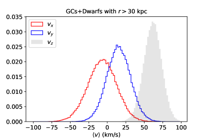
Figure 6: Mean velocity in sample of 33 globular clusters and dwarfs with galactocentric distances larger than 30 kpc. This shows that these satellites have a substantial velocity shift relative to the Milky Way. This could be due to the reflex motion induced by the LMC or due to substrcture and phase-space correlation amongst the satellites.

Along similar lines, we note that Gilbert et al. (2018) has shown that there is a significant velocity offset between the stellar halo and disk in Andromeda (see Fig. 7 of that work). Such an offset could arise from an interaction between Andromeda and a large satellite as in this work. Thus, this may be due to the recent merger proposed by Hammer et al. (2018).

3.2 Leo I

The large relative speed of the Leo I dwarf galaxy relative to the Milky Way (Sohn et al., 2013) has been used to constrain the mass of the Milky Way (Boylan-Kolchin et al., 2013) assuming that it is bound to our Galaxy. However, since the outer parts of our Galaxy are out of equilibrium, this relative speed already includes the additional reflex motion imparted by the LMC. In order to assess the impact of the LMC on Leo I we take two approaches. First, we estimate this reflex motion using the fiducial simulations from Section 2 with an LMC mass of $1.5\times 10^{11}M_{\odot}$. We take the mean velocity of all particles within 2 degrees on the sky and 30 kpc along the line of sight from the currently measured location of Leo I. Accounting for the reflex motion, the relative speed of Leo I drops from $\sim 197$ km/s to $\sim 168$ km/s.

Second, we integrate the orbit of Leo I in the presence of the LMC using the machinery from Erkal & Belokurov (2019). Namely, we rewind Leo I back in time for 5 Gyr (or until the LMC has an apocenter, whichever is sooner) including the effect of a $1.5\times 10^{11}M_{\odot}$ LMC. The Milky Way and LMC potentials are the same as in Section 2. We Monte Carlo the present day positions and velocities of the LMC and Leo I 10,000 times and compare the energy of Leo I relative to the Milky Way at the present and 5 Gyr ago (i.e. before the infall of the LMC). We find that the energy of Leo I was substantially lower (i.e. it was substantially more bound) before the infall of the LMC. In order to facilitate the comparison with Boylan-Kolchin et al. (2013), we convert this energy difference into a change of the velocity of Leo I. Thus, we find that if Leo I was observed at its current location before the infall of the LMC, it would have had a speed of $\sim 169$ km/s relative to the Milky Way. This is much lower than its present day relative speed of $\sim 197$ km/s.

Interestingly, both approaches give nearly the same result showing consistently that a significant portion of Leo I’s speed is due to the LMC. In terms of the results of Boylan-Kolchin et al. (2013), this $\sim 15\%$ decrease in the speed is a slightly larger effect than changing the Milky Way mass from $10^{12}M_{\odot}$ to $1.5\times 10^{12}M_{\odot}$ which results in a $\sim 13\%$ reduction in $v/v_{\rm vir}$. This suggests that if the analysis of Boylan-Kolchin et al. (2013) was repeated accounting for a $1.5\times 10^{11}M_{\odot}$ LMC, the inferred Milky Way mass would be close to $\sim 10^{12}M_{\odot}$.

3.3 Conclusions

In this work we have shown that the LMC should push the outskirts of our Galaxy substantially out of equilibrium. In particular, the leading order effect of the LMC is that the inner parts of the Milky Way nearly decouple from the region beyond $\sim 30$ kpc. Thus, observations of populations beyond $\sim 30$ kpc should show signs of this near-bulk motion. Importantly, we demonstrated how this disequilibrium affects models of matter distribution in the outer parts of our Galaxy using the mass estimator of Watkins, Evans & An (2010). The systematic bias in the tracer velocity dispersion induces the mass bias which is always positive and can be as large as $\sim 50\%$ depending on the mass of the LMC. We showed that this bias depends on where the tracers are located and that certain parts of the sky offer a substantially improved estimate. This bias can also be reduced if the mean reflex motion is accounted for. In a similar vein, we showed that the LMC significantly increases the present-day speed of Leo I relative to the Milky Way and that if this is accounted for, the Milky Way mass estimate of Boylan-Kolchin et al. (2013) will be significantly lower.

Accounting for the reflex motion induced by the LMC may also bring into closer agreement the different mass estimates for the Milky Way (e.g. Bland-Hawthorn & Gerhard, 2016; Wang et al., 2019) which are made with tracers at different radii and using different techniques. Based on the results of this work, the estimates made with data in the outskirts of our Galaxy are likely biased high due to the nearly bulk motion beyond $\sim 30$ kpc. Future observations of the stellar halo with Gaia DR3, as well as upcoming radial velocity surveys like WEAVE and 4MOST, will allow us to measure this bulk motion and determine how significant this effect is.

References

- Al Sufi (964) Al Sufi A., 964, Book of Fixed Stars, Isfahan, Persia
- Astropy Collaboration et al. (2013) Astropy Collaboration et al., 2013, A&A, 558, A33
- Avner & King (1967) Avner E. S., King I. R., 1967, AJ, 72, 650
- Belokurov et al. (2019) Belokurov V., Deason A. J., Erkal D., Koposov S. E., Carballo-Bello J. A., Smith M. C., Jethwa P., Navarrete C., 2019, MNRAS, 488, L47
- Besla et al. (2007) Besla G., Kallivayalil N., Hernquist L., Robertson B., Cox T. J., van der Marel R. P., Alcock C., 2007, ApJ, 668, 949
- Bland-Hawthorn & Gerhard (2016) Bland-Hawthorn J., Gerhard O., 2016, ARA&A, 54, 529
- Bovy (2015) Bovy J., 2015, ApJS, 216, 29
- Boylan-Kolchin et al. (2013) Boylan-Kolchin M., Bullock J. S., Sohn S. T., Besla G., van der Marel R. P., 2013, ApJ, 768, 140
- Burke (1957) Burke B. F., 1957, AJ, 62, 90
- Correnti et al. (2018) Correnti M., Gennaro M., Kalirai J. S., Cohen R. E., Brown T. M., 2018, ApJ, 864, 147
- Erkal et al. (2019) Erkal D. et al., 2019, MNRAS, 487, 2685
- Erkal & Belokurov (2019) Erkal D., Belokurov V. A., 2019, arXiv e-prints, arXiv:1907.09484
- Fritz et al. (2020) Fritz T. K., Di Cintio A., Battaglia G., Brook C., Taibi S., 2020, arXiv e-prints, arXiv:2001.02651
- Gaia Collaboration et al. (2018) Gaia Collaboration et al., 2018, A&A, 616, A12
- Garavito-Camargo et al. (2019) Garavito-Camargo N., Besla G., Laporte C. F. P., Johnston K. V., Gómez F. A., Watkins L. L., 2019, ApJ, 884, 51
- Gardner, Hinkel & Yanny (2020) Gardner S., Hinkel A., Yanny B., 2020, arXiv e-prints, arXiv:2001.01399
- Gilbert et al. (2018) Gilbert K. M. et al., 2018, ApJ, 852, 128
- Gómez et al. (2015) Gómez F. A., Besla G., Carpintero D. D., Villalobos Á., O’Shea B. W., Bell E. F., 2015, ApJ, 802, 128
- Gratton et al. (2003) Gratton R. G., Bragaglia A., Carretta E., Clementini G., Desidera S., Grundahl F., Lucatello S., 2003, A&A, 408, 529
- Gravity Collaboration et al. (2018) Gravity Collaboration et al., 2018, A&A, 615, L15
- Hammer et al. (2018) Hammer F., Yang Y. B., Wang J. L., Ibata R., Flores H., Puech M., 2018, MNRAS, 475, 2754
- Hernquist (1990) Hernquist L., 1990, ApJ, 356, 359
- Hunter (2007) Hunter J. D., 2007, Computing in Science Engineering, 9, 90
- Jones et al. (2001–) Jones E., Oliphant T., Peterson P., et al., 2001–, SciPy: Open source scientific tools for Python. http://www.scipy.org/
- Kallivayalil et al. (2018) Kallivayalil N. et al., 2018, ApJ, 867, 19
- Kallivayalil, van der Marel & Alcock (2006) Kallivayalil N., van der Marel R. P., Alcock C., 2006, ApJ, 652, 1213
- Kallivayalil et al. (2013) Kallivayalil N., van der Marel R. P., Besla G., Anderson J., Alcock C., 2013, ApJ, 764, 161
- Kerr (1957) Kerr F. J., 1957, AJ, 62, 93
- Kirby et al. (2013) Kirby E. N., Boylan-Kolchin M., Cohen J. G., Geha M., Bullock J. S., Kaplinghat M., 2013, ApJ, 770, 16
- Kirby et al. (2017) Kirby E. N., Cohen J. G., Simon J. D., Guhathakurta P., Thygesen A. O., Duggan G. E., 2017, ApJ, 838, 83
- Koposov et al. (2011) Koposov S. E. et al., 2011, ApJ, 736, 146
- Lancaster et al. (2019) Lancaster L., Koposov S. E., Belokurov V., Evans N. W., Deason A. J., 2019, MNRAS, 486, 378
- Laporte et al. (2018) Laporte C. F. P., Gómez F. A., Besla G., Johnston K. V., Garavito-Camargo N., 2018, MNRAS, 473, 1218
- Martin et al. (2016) Martin N. F. et al., 2016, MNRAS, 458, L59
- Moster, Naab & White (2013) Moster B. P., Naab T., White S. D. M., 2013, MNRAS, 428, 3121
- Pace & Li (2019) Pace A. B., Li T. S., 2019, ApJ, 875, 77
- Patel et al. (2020) Patel E. et al., 2020, arXiv e-prints, arXiv:2001.01746
- Peñarrubia et al. (2016) Peñarrubia J., Gómez F. A., Besla G., Erkal D., Ma Y.-Z., 2016, MNRAS, 456, L54
- Perez & Granger (2007) Perez F., Granger B. E., 2007, Computing in Science Engineering, 9, 21
- Petersen & Peñarrubia (2020) Petersen M. S., Peñarrubia J., 2020, arXiv e-prints, arXiv:2001.09142
- Piatek, Pryor & Olszewski (2016) Piatek S., Pryor C., Olszewski E. W., 2016, AJ, 152, 166
- Posti et al. (2015) Posti L., Binney J., Nipoti C., Ciotti L., 2015, MNRAS, 447, 3060
- Price-Whelan et al. (2018) Price-Whelan A. M. et al., 2018, AJ, 156, 123
- Simon (2018) Simon J. D., 2018, ApJ, 863, 89
- Simon & Geha (2007) Simon J. D., Geha M., 2007, ApJ, 670, 313
- Simon et al. (2017) Simon J. D. et al., 2017, ApJ, 838, 11
- Sohn et al. (2013) Sohn S. T., Besla G., van der Marel R. P., Boylan-Kolchin M., Majewski S. R., Bullock J. S., 2013, ApJ, 768, 139
- Sohn et al. (2018a) Sohn S. T., Watkins L. L., Fardal M. A., van der Marel R. P., Deason A. J., Besla G., Bellini A., 2018a, ApJ, 862, 52
- Sohn et al. (2018b) Sohn S. T., Watkins L. L., Fardal M. A., van der Marel R. P., Deason A. J., Besla G., Bellini A., 2018b, ApJ, 862, 52
- Torrealba et al. (2019) Torrealba G. et al., 2019, MNRAS, 488, 2743
- van der Walt, Colbert & Varoquaux (2011) van der Walt S., Colbert S. C., Varoquaux G., 2011, Computing in Science Engineering, 13, 22
- Vasiliev (2019a) Vasiliev E., 2019a, MNRAS, 482, 1525
- Vasiliev (2019b) Vasiliev E., 2019b, MNRAS, 484, 2832
- Walker et al. (2016) Walker M. G. et al., 2016, ApJ, 819, 53
- Wang et al. (2019) Wang W., Han J., Cautun M., Li Z., Ishigaki M. N., 2019, arXiv e-prints, arXiv:1912.02599
- Watkins, Evans & An (2010) Watkins L. L., Evans N. W., An J. H., 2010, MNRAS, 406, 264
- Watkins et al. (2009) Watkins L. L. et al., 2009, MNRAS, 398, 1757
- Watkins et al. (2019) Watkins L. L., van der Marel R. P., Sohn S. T., Evans N. W., 2019, ApJ, 873, 118
- Willman et al. (2011) Willman B., Geha M., Strader J., Strigari L. E., Simon J. D., Kirby E., Ho N., Warres A., 2011, AJ, 142, 128