Scale and Scheme Variations in Unitarized NLO Merging

Abstract

Precision background predictions with well-defined uncertainty estimates are important for interpreting collider-physics measurements and for planning future high-energy collider experiments. It is especially important to estimate the perturbative uncertainties in predictions of inclusive measurements of jet observables, that are designed to be largely insensitive to non-perturbative effects such as the structure of beam-remnants, multi-parton scattering or hadronization. In this study, we discuss possible pit-falls in defining the perturbative uncertainty of unitarized next-to-leading order multi-jet merged predictions, using the Pythia event generator as our vehicle. For this purpose, we consider different choices of unitarized NLO merging schemes as well as consistent variations of renormalization scales in different parts of the calculation. Such a combined discussion allows to rank the contribution of scale variations to the error budget in comparison to other contributions due to algorithmic choices that are often assumed fixed. The scale uncertainty bands of different merging schemes largely overlap, but differences between the “central” predictions in different schemes can remain comparable to scale uncertainties even for very well-separated jets, or be larger than scale uncertainties in transition regions between calculations of different jet multiplicity. The availability of these variations within Pythia will enable more systematic studies of perturbative uncertainties in precision background calculations in the future.

I Introduction

Precision predictions of the final states of high-energy scattering signal or background processes are crucial for the continued success of high-energy collider physics. This includes e.g. exploiting the potential of indirect searches for physics beyond the Standard Model (SM) at the Large Hadron Collider, or precision SM measurements at future lepton colliders. The more detailed signal and background final states can be predicted, the larger the set of conceivable measurements. General-Purpose Event generators (GPEGs) Buckley:2011ms produce a detailed description of final states at the level of individual particles, and thus provide controlled pseudo-data (in the form of simulated scattering events) that can be used to develop new analysis strategies. At the same time, GPEGs aim to predict moderately exclusive final states with as high precision as possible, such that precision SM predictions can be juxtaposed with data to allow setting exclusion limits on parameters in Beyond-the-SM theories.

The precision of GPEG simulations is typically difficult to quantify, since the calculations are based on a mix of perturbative calculations (to determine the distribution of the highest-energy transfer scattering, and its radiative cascade) and phenomenological models, which are necessary to describe the scattering final state in detail (e.g. to incorporate the remnants of colliding beams after scattering, and to ensure conservation of momentum, electric, and QCD color charges). Some measurements are constructed to be as insensitive as possible to phenomenological beam-remnant, multi-particle scattering or hadronization models, such that the uncertainties due to perturbative approximations dominate the overall error budget. Measurements in this category are very inclusive measurements of inelastic scattering processes that do not, at lowest order, include QCD couplings, or moderately inclusive measurements constructed with the help of infrared safe observables.

The goal of this work is to discuss, define and assess the contribution of uncertainties due to perturbative approximations to the error budget of predictions to multi-jet final states at colliders, using precise next-to-leading (NLO) multi-jet merged predictions within the Pythia event generator Sjostrand:2006za ; Sjostrand:2014zea as a case study. Similar case studies within individual leading-order or NLO matched predictions have been considered in Bellm:2016rhh ; Cormier:2018tog , while Bothmann:2016nao focussed on the technical validation of variations within a specific NLO merging scheme. We extend these discussions by considering the combination of several NLO calculations (a particular scheme of combining NLO calculations will define what we call an NLO merging scheme), and the uncertainty due to choices in the combination procedure, i.e. the merging scheme. In particular, we focus on the interplay of uncertainties from defining exclusive cross sections at higher orders, and scale variations within unitarized merging schemes, thus addressing the questions: What is the impact of choices that are not constrained by requirements from retaining shower- and/or fixed-order accuracy on the prediction and uncertainty of the overall calculation? Do some merging schemes exhibit spuriously sized scale uncertainties?

II Unitarized NLO-merged calculations

Scattering events at high-energy colliders such as the LHC potentially contain many well-separated jets of particles. To obtain a sound perturbative model in such a situation, several precise fixed-order calculations are necessary to supplement the parton shower, which, due to its ordering requirement, cannot reach all regions of phase space. Since the parton shower also relies on approximate collinear/soft splitting kernels, its model of hard well-separated jets is typically insufficient. Disregarding hard regions can affect the overall event generator tune, since they can e.g. significantly alter the description of large particle-multiplicty tails.

Thus, several calculations (that are themselves combinations of fixed-order and all-order perturbative components) need to be combined. We will refer to a combination scheme as merging scheme. The prerequisite for these are matrix-element generators that can readily provide the necessary fixed-order calculations. Fixed-order calculations with light final-state partons require regularization to avoid infrared singularities. This regularization can be achieved by removing all phase-space regions for which the value of a kinematically defined merging scale falls below a pre-defined value. Events that were thus discarded can be recovered by subsequent parton showering. Thus, the merging scale takes on a two-fold meaning: It acts as regularization of fixed-order calculations, and as a separator between fixed-order- and parton shower phase space regions. Since the merging scale definition and value are not unique, this introduces an algorithmic uncertainty into merging schemes. The aim of the current study will be to investigate the interplay between theoretically unavoidable uncertainties due to truncation of the perturbative series, and higher-order uncertainties in the definition of the merging prescription. This interplay can be obscured by varying other algorithmic choices such as the merging scale. To avoid inconclusive statements, we will thus not consider such variations below.

Merging schemes rely on consistency conditions designed to ensure that the precision of none of their parts is degraded: In the phase-space regions in which fixed-order calculations are supplemented, the fixed-order expansion of the merged prediction should recover the original calculation, while throughout the phase-space available to showering, the all-order results should recover parton-shower resummation. The interplay between these requirements is especially delicate in “transition regions”, where several components contribute almost equally to the final result, and in “non-shower regions” beyond the reach of (ordered) showering, for which no comprehensive all-order description is known.

A straight-forward consistency constraint can be obtained from the unitary nature of the parton shower, i.e. that the sum of exclusive $n$-parton cross section and inclusive $n+1$-parton cross section recovers the inclusive $n$-parton cross section for observables only sensitive to $n$ partons. We can extend this property also to merged calculations, thus arriving at unitarized merging schemes Rubin:2010xp ; Lonnblad:2012ng ; Lonnblad:2012ix ; Platzer:2012bs ; Bellm:2017ktr .

Unitarized NLO merging schemes enforce consistency between different calculations by removing the complete impact of newly added high-parton-multiplicity configurations from the inclusive prediction by explicit subtraction of reduced-multiplicity counter-events,

$$\langle\mathcal{O}\rangle_{n} =~{}\Big{(}\textnormal{(inclusive rate for $n$ partons)}[\Phi_{n}]-\textnormal{(inclusive rate for $n+1$ partons)}[\Phi_{n+1}]\Big{)}\mathcal{O}_{n}[\Phi_{n}]$$ (1)

$$+~{}~{}\,\,\textnormal{(inclusive rate for $n+1$ partons)}[\Phi_{n+1}]\mathcal{O}_{n+1}[\Phi_{n+1}]$$

where $\mathcal{O}_{n}$ denotes a fully differential measurement of all momenta in the state $\Phi_{n}]$. In reality, this complete removal is only achieved for very specific observables (e.g. jet observables defined by using the merging scale definition as separation criterion, and the inverse of the parton shower kinematics as recombination scheme), while residual higher-multiplicty sensitivity remains in observables very different to the fixed-order regularization cut. Nevertheless, the same cancellation should in principle also apply to the uncertainty on the high-parton-multiplicity configurations. The latter requires very careful handling of all components of the calculation.

A sensible inclusive prediction should also be complemented with an accurate description of exclusive cross sections that are sensitive to exactly $n$ (and only $n$) jets or partons. Unitarization introduces higher-order components that depend on higher-parton-multiplicities into exclusive cross sections, by means of the explicit subtraction, i.e. through the second term in eq. 1. These differ from the naive parton-shower result by subleading terms in the parton-shower evolution variable. At NLO, similar subleading terms can appear by introducing all-order corrections to (hard) virtual diagrams, i.e. through the first term in eq. 1. The interplay of these terms is beyond both NLO fixed-order accuracy as well as shower accuracy. However, it is of the same order as variations that are used to gauge NLO fixed-order uncertainties.

It is prudent to require a merged calculation to recover the fixed-order result as well as the uncertainty of the latter in certain regions of phase-space. However, it is not a priori clear how these regions should be defined, nor that it is obvious that any merging scheme (taken here to be defined by different choices of reweighting the NLO corrections) fulfills this requirement. The aim of the current pilot study is to initiate the discussion of these points. To be able to discuss subtle changes in the NLO merged event generator predictions by using a (large) fixed set of statistically produced events, we focus on “reweightable variations” here, such that the impact of purely statistical fluctuations can be minimized. Possible reweightable perturbative variations are

• Variations of the renormalization scale, correlated between fixed-order and parton-shower components;

• Variations of the (all-order) reweighting of higher-order fixed-order terms.

Many other variations are of course possible in an NLO merged calculation. However, these might not be reweightable and thus require prohibitively large event samples to minimize statistical effects, or do not have a well-defined perturbative expansion. Hence, the current study is limited to a consistent definition and assessment of the variations $a)$ and $b)$ above. Other variations (such as factorization scale changes) will not invalidate the findings below, and instead might serve to put more stringent constraints on the allowed form of NLO merging schemes.

III Theory and Implementation

In this section, we define several variants of unitarized NLO merging strategies that have well-motivated, yet different, higher-order structure. For this, we will start from a very general form of a unitarized merging prescription, of which the UNLOPS prescriptions Lonnblad:2012ix and Bellm:2017ktr are sub-sets. This general starting point allows to define several classes of unitarized NLO merging schemes, and thus suggests a large associated uncertainty. However, most unitarized NLO merging schemes will have a spurious behavior, e.g. if their all-order behavior does not recover the all-order logarithmic structure of QCD. Thus, we will discuss conditions that sensible new unitarized NLO merging schemes need to fulfill, e.g. how to define schemes in which scale uncertainties do not deteriorate the accuracy of the overall prediction. The result of this is that we allow a new source of uncertainty – the scheme uncertainty – and determine sensible scheme variations that may constitute a reasonable assessment of this uncertainty.

To begin, it is useful to examine the construction of exclusive jet rates in the merged calculation, with the exclusive 1-jet rate being a sufficiently complicated example. In a general unitarized calculation, this rate is given by

$$\langle\mathcal{O}_{1}\rangle=\mathcal{O}_{1}[\Phi_{1}] \Bigg{(}\left(\mathds{B}_{1}[\Phi_{1}]+\mathds{B}_{1}^{\text{NLO}}[\Phi_{1}]\right)w_{\text{NLO}}[\Phi_{0},\Phi_{1}]+\mathds{B}_{1}[\Phi_{1}]\left(w_{\text{LO}}[\Phi_{0},\Phi_{1}]-w_{\text{I}}[\Phi_{0}]-w_{\text{S}}[\Phi_{0},\Phi_{1}]\alpha_{s}\left\{w_{\text{LO}}[\Phi_{0},\Phi_{1}]\right\}_{1}\right)$$ (2)

$$-\int_{t_{\mathrm{ms}}}\mathds{B}_{2}[\Phi_{2}]w_{\text{LO}}[\Phi_{0}^{\prime},\Phi_{1}^{\prime}]w_{\text{LO}}[\Phi_{1},\Phi_{2}]-S_{3}\Bigg{)}$$

where the factors $w_{\text{X}}$ are a-priori weights that have to be chosen to preserve certain accuracy criteria, $\mathds{B}_{i}[\Phi_{i}]$ denote the inclusive tree-level calculation of the $i$-jet rate, $\mathds{B}_{1}^{\text{NLO}}[\Phi_{1}]$ all NLO corrections (including all virtual and real corrections) to the 1-jet rate, and where we have collected pieces stemming from the unitarization of higher-multiplicity contributions with lowest order $\alpha_{s}^{3}$ into the symbol $S_{3}$. We assume that all factors $w_{\text{X}}$ have a well-defined expansion

$$w_{\text{X}}(\mu_{r})=\sum_{i=0}^{\infty}\alpha_{s}^{i}\left\{w_{\text{X}}\right\}_{i}=1+\alpha_{s}(\mu_{r})\left\{w_{\text{X}}\right\}_{1}+\alpha_{s}^{2}(\mu_{r})\left\{w_{\text{X}}\right\}_{2}+\mathcal{O}(\alpha_{s}^{3})$$ (3)

This expansion immediately guarantees that the lowest-order terms in the expansion of eq. 2 is correctly given by the tree-level result $\mathcal{O}_{1}[\Phi_{1}]\mathds{B}_{1}[\Phi_{1}]$. Similarly, the next term in the expansion is correctly given by the exclusive NLO cross section

$$\langle\mathcal{O}_{1}\rangle^{(2)}=\mathcal{O}_{1}[\Phi_{1}]\left(\mathds{B}_{1}^{NLO}[\Phi_{1}]-\int_{t_{\mathrm{ms}}}\mathds{B}_{2}[\Phi_{2}]\right)=\mathcal{O}_{1}[\Phi_{1}]\left(V_{1}[\Phi_{1}]+\int^{t_{\mathrm{ms}}}\mathds{B}_{2}[\Phi_{2}]\right)$$ (4)

provided that $\left\{w_{\text{NLO}}\right\}_{1}=\left\{w_{\text{I}}\right\}_{1}$ and that the real corrections in $\mathds{B}_{1}^{\text{NLO}}$ and the unitarization term $\int_{t_{\mathrm{ms}}}\mathds{B}_{2}$ are mapped in an identical way to the $\Phi_{1}$ phase space points. Non-unitarized merging schemes arrive at the exclusive NLO cross section in a somewhat different manner Hoeche:2012yf .

Note that to achieve the correct behavior for any choice of the renormalization scale requires $\left\{w_{\text{NLO}}\right\}_{1}=\left\{w_{I}\right\}_{1}$ for each scale value, and thus implies that the expansion of either weight can be defined with reference to a common scale, and that

$$w_{\text{X}}(\mu_{r})-w_{\text{X}}(k\mu_{r})=\alpha_{s}^{2}(\mu_{r})\frac{\beta_{0}}{2\pi}\ln(k)\left\{w_{\text{X}}\right\}_{1}+\mathcal{O}(\alpha_{s}^{3})\quad\text{X}\in\{\text{NLO},\text{I}\}\,.$$ (5)

If this condition is not guaranteed, then the all-order accuracy of the prediction, as defined by reference to the parton shower, is compromised. Changes due to scale variations of weights applied to Born-level contributions enter at the same order ($\mathcal{O}(\alpha_{s}^{3})$) as a non-trivial reweighting of higher-order (virtual) corrections. The interplay between these corrections is the main interest of this article. In order to avoid over-generalizations of conclusions about uncertainties drawn from scale variations, we will analyse the $\mathcal{O}(\alpha_{s}^{3})$ expansion of eq. 2 and set up conditions for the reweighting of higher-order corrections. Any reweighting must not, of course, introduce spurious enhacements at any order, since this would exaggerate the “scheme variation”. With this in mind, different reweighting strategies can be used together with scale variations to determine more robust uncertainties.

The $\mathcal{O}(\alpha_{s}^{3})$ expansion of eq. 2 reads Lonnblad:2012ix

$$\langle\mathcal{O}_{1}\rangle^{(3)}= \mathcal{O}_{1}[\Phi_{1}]\Bigg{(}\left\{w_{\text{NLO}}\right\}_{2}\mathds{B}_{1}+\left\{w_{\text{NLO}}\right\}_{1}\mathds{B}_{1}^{\text{NLO}}+\left\{w_{\text{LO}}\right\}_{2}\mathds{B}_{1}-\left\{w_{\text{I}}\right\}_{2}\mathds{B}_{1}-\left\{w_{\text{S}}\right\}_{1}\left\{w_{\text{LO}}\right\}_{1}\mathds{B}_{1}$$ (6)

$$\quad\qquad-\int_{t_{\mathrm{ms}}}\Bigg{(}\mathds{B}_{2}^{\text{NLO}}-\int\mathds{B}_{3}^{\downarrow}\Bigg{)}\Bigg{)}~{},$$

where we have explicitly included the relevant $S_{3}$ terms and assumed that $\left\{w_{\text{NLO}}\right\}_{1}=\left\{w_{\text{I}}\right\}_{1}$ also applies to the reweighting of two-parton corrections.

It is reasonable to expect that eq. 6 reproduces the correct coefficient of the largest contribution for the observable $\mathcal{O}_{1}[\Phi_{1}]$. If the observable measures the merging scale value of states in $\Phi_{1}$, we expect a behavior $\mathcal{O}_{1}^{(3)}\propto\alpha_{s}^{3}\ln^{6}(t_{\mathrm{ms}})$. Since $\left\{w_{\text{LO}}\right\}_{2}\mathds{B}_{1}\propto\alpha_{s}^{3}\ln^{6}(t_{\mathrm{ms}})$, this amounts to constraints on and/or cancellations between the different weights in eq. 6. The most straight-forward way to enforce such cancellations is to set $w_{\text{NLO}}=w_{\text{I}}$ for any scale value (we have already seen that this holds for the lowest and next-to-lowest order), and then constrain the concrete form of $w_{\text{NLO}}$ from the remaining terms. If we assume that $\left\{w_{\text{LO}}\right\}_{1}\mathds{B}_{1}$ provides a sensible approximation of the leading parts of $\mathds{B}_{1}^{\text{NLO}}$, it is tempting to identify

$$\left\{w_{\text{NLO}}\right\}_{1}\mathds{B}_{1}^{\text{NLO}}-\left\{w_{\text{S}}\right\}_{1}\left\{w_{\text{LO}}\right\}_{1}\mathds{B}_{1}\longrightarrow\left\{w\right\}_{1}\left[\mathds{B}_{1}^{\text{NLO}}-\left\{w_{\text{LO}}\right\}_{1}\mathds{B}_{1}\right]\quad\textnormal{i.e.}\quad\left\{w_{\text{S}}\right\}_{1}=\left\{w_{\text{NLO}}\right\}_{1}=\left\{w\right\}_{1}(=\left\{w_{\text{I}}\right\}_{1})~{}.$$ (7)

As long as $\left\{w\right\}_{1}$ scales as $\alpha_{s}\ln^{2}(t_{\mathrm{ms}})$ or less, and while the difference in brackets is subleading, this combination will not lead to undesirable enhancements. Nevertheless, while $\left\{w\right\}_{1}\neq 0$ and $\mathds{B}_{1}^{\text{NLO}}\neq\left\{w_{\text{LO}}\right\}_{1}\mathds{B}_{1}$, this contribution is a new, process-dependent, source of scale uncertainties beyond the NLO and parton shower approximations. The impact of this term on the overall uncertainty is thus best estimated by considering explicit test cases, as e.g. done in the next section. It could be argued that having $w\not\equiv 1$ brings the merging prescription closer to the traditional separation into all-order $W$-terms and fixed-order $Y-$terms in analytic resummation Collins:1981va ; Collins:1984kg , which typically includes hard virtual corrections into the all-order $W$-term Collins:1981uk and assumes that the fixed-order $Y$-term not only remains constant, but vanishes in the limit when $\Phi_{1}$ and $\Phi_{2}$ become indistinguishable Catani:2010pd . It is however not directly obvious that the calculation in Collins:1981uk translates to the context of a fully differential event generator employing IR/UV regularization prescriptions different from Collins:1981uk . An assessment of the numerical effect of different treatments is thus interesting in its own right, also beyond the context of its interplay with renormalization scale variations in NLO merging schemes.

To summarize, the above considerations lead to a simple guideline how higher-order corrections may be reweighted without compromising the quality of the calculation: All terms in the expansion of the leading-order reweighting $w_{\text{LO}}$, and all NLO corrections, should be reweighted by the same (potentially dynamical) weight. Enhancements appearing in the expansion of this weight should be in agreement with standard QCD expectations. Below, we describe different unitarized NLO merging strategies that meet these criteria. We then assess the uncertainties on predictions that result from consistent renormalization scale variations in matrix element generation, merging and parton shower, as well as the “merging scheme” uncertainty. We limit the discussion to predictions that are NLO correct up to the first additional jet with respect to the reference process, and LO correct for the second and third jet. The generalization to higher multiplicity is straight forward, but omitted here in favor of readability.

III.1 UNLOPS

We start from the UNLOPS multi-leg NLO merging scheme described in detail in Lonnblad:2012ix . The expectation value of an arbitrary jet observable $\mathcal{O}$ in UNLOPS is given by

$$\mathcal{O}_{0} \left(\bar{\mathds{B}}_{0}-\int\mathds{B}_{1}\left(\Pi_{0}(k)w_{f,0}\frac{\alpha_{s}(kp_{\perp,1})}{\alpha_{s}(k\mu_{\mathrm{R}})}K-1-\left\{\Pi_{0}(k)\right\}_{\alpha_{s}(k\mu_{\mathrm{R}})}-\{w_{f,0}\}_{\alpha_{s}(k\mu_{\mathrm{R}})}-\left\{\frac{\alpha_{s}(kp_{\perp,1})}{\alpha_{s}(k\mu_{\mathrm{R}})}\right\}_{\alpha_{s}(k\mu_{\mathrm{R}})}-\{K\}_{\alpha_{s}(\mu_{\mathrm{R}})}\right)\right.$$ (8)

$$\left.-\int\bar{\mathds{B}}_{1}\right)$$

$$+\mathcal{O}_{1} \left(\bar{\mathds{B}}_{1}+\mathds{B}_{1}\left(\Pi_{0}(k)w_{f,0}\frac{\alpha_{s}(kp_{\perp,1})}{\alpha_{s}(k\mu_{\mathrm{R}})}K-1-\left\{\Pi_{0}(k)\right\}_{\alpha_{s}(k\mu_{\mathrm{R}})}-\{w_{f,0}\}_{\alpha_{s}(k\mu_{\mathrm{R}})}-\left\{\frac{\alpha_{s}(kp_{\perp,1})}{\alpha_{s}(k\mu_{\mathrm{R}})}\right\}_{\alpha_{s}(k\mu_{\mathrm{R}})}-\{K\}_{\alpha_{s}(\mu_{\mathrm{R}})}\right)\right.$$

$$\left.-\int\mathds{B}_{2}\Pi_{0}(k)w_{f,0}\frac{\alpha_{s}(kp_{\perp,1})}{\alpha_{s}(k\mu_{\mathrm{R}})}\Pi_{1}(k)w_{f,1}\frac{\alpha_{s}(kp_{\perp,2})}{\alpha_{s}(k\mu_{\mathrm{R}})}K\right)$$

$$+\mathcal{O}_{2} \int\mathds{B}_{2}\Pi_{0}(k)w_{f,0}\frac{\alpha_{s}(kp_{\perp,1})}{\alpha_{s}(k\mu_{\mathrm{R}})}\Pi_{1}(k)w_{f,1}\frac{\alpha_{s}(kp_{\perp,2})}{\alpha_{s}(k\mu_{\mathrm{R}})}K\,.$$

with $k=1$. In the above equation, $\mathds{B}$ and $\bar{\mathds{B}}$ denote fully differential cross sections at leading and next-to-leading order in the strong coupling, in the following also called matrix element samples. These are interfaced using the LHEF format. $\{X\}_{\alpha_{\mathrm{s}}}$ denotes the $\mathcal{O}(\alpha_{\mathrm{s}})$ contribution to the term $X$. $\Pi_{n}(k)$ is short for

$$\Pi_{n}(p_{\perp,n},p_{\perp,n+1};x,k)=\prod_{j}\exp\left\{-\sum_{i}\int_{p_{\perp,n+1}}^{p_{\perp,n}}\frac{\text{d}p_{\perp}^{2}}{p_{\perp}^{2}}\int\frac{\text{d}z}{z}\frac{\alpha_{s}(kp_{\perp})}{2\pi}P_{ji}(z)\frac{f_{i}(x/z,p_{\perp})}{f_{j}(x,p_{\perp})}\right\}$$ (9)

and describes the no-emission probability between the two evolution scales, taking into account all allowed $i\rightarrow j$ splittings of all legs in an $n$ parton state, as described by the kernels $P_{ji}(z)$. This no-emission probability can be calculated numerically by trial parton showering Lonnblad:2001iq . In Pythia 8 Sjostrand:2014zea , where the evolution of partons by emissions and the simulation of secondary multiparton interactions (MPI) is described by a common, interleaved, evolution sequence, the no-emission probabilities generated by trial showering can also accommodate no-MPI probabilities of the relevant transverse momentum scales Lonnblad:2011xx . This allows a smooth combination of input matrix element samples with the MPI machinery.

In case of hadronic initial states, the necessary PDF ratios

$$w_{f,n}=\frac{x_{n}^{+}f_{n}^{+}(x_{n}^{+},p_{\perp,n})}{x_{n}^{+}f_{n}^{+}(x_{n}^{+},\mu_{F})}\frac{x_{n}^{-}f_{n}^{-}(x_{n}^{-},p_{\perp,n})}{x_{n}^{-}f_{n}^{-}(x_{n}^{-},\mu_{F})}\prod_{i=1}^{n}\frac{x_{i-1}^{+}f_{i-1}^{+}(x_{i-1}^{+},p_{\perp,{i-1}})}{x_{i-1}^{+}f_{i-1}^{+}(x_{i-1}^{+},p_{\perp,i})}\frac{x_{i-1}^{-}f_{i-1}^{-}(x_{i-1}^{-},p_{\perp,{i-1}})}{x_{i-1}^{-}f_{i-1}^{-}(x_{i-1}^{-},p_{\perp,i})}$$ (10)

are included as additional weights. As argued above, we do not vary the factorization scale, since it is not obvious how to achieve a consistent reweightable variation in this case. The subscript on $\mathcal{O}_{n}$ denotes the final state multiplicity of the states handed to subsequent event generation steps. Thus, in some cases, e.g. to create counter-events for unitarization, the state used to evaluate the matrix element calculation is replaced by a lower-multiplicty state determined by reclustering according to a reconstructed parton shower history. Finally, the $K$-factor is only applied to configurations that could have been produced by parton shower emissions. These regions are defined by being able to construct at least one parton shower history of emissions that are ordered in a decreasing sequence of evolution scales. This choice is consistent with the MC@NLO matching scheme, where hard real-emission configurations not reachable by showering are described with tree-level matrix elements.

Note that in this UNLOPS scheme, we set $w_{S}=w_{NLO}=w_{I}\equiv 1$, i.e. treat all higher-order fixed-order corrections as “hard corrections” that do not contribute to the all-order result. This relatively conservative approach has the advantage that scale variations due to “hard” virtual corrections do not introduce all-order uncertainties. It has the disadvantage that any “soft” virtual correction terms in $\mathds{B}_{1}^{NLO}$ that are not correctly reproduced by the parton shower are not leveraged to define a more realistic all-order uncertainty.

We may estimate the theoretical uncertainties of predictions obtained by the UNLOPS NLO merging procedure by variations of the renormalization scale $\mu_{\mathrm{R}}$. For consistency, these variations should not be limited to the seed cross sections, but should also include renormalization scale variations of the parton shower. For this reason, we employ the scale variations that have been implemented in the Pythia 8 parton shower Mrenna:2016sih . We extend this procedure to ensure consistent simultaneous variations in the calculation of merging weights, and a consistent set-up between matrix-element and parton-shower contributions. Every renormalization scale in the matrix element samples $\mathds{B}_{n}$, $\bar{\mathds{B}}_{n}$ is varied, as is every explicit occurrence of $\mu_{\mathrm{R}}$ in the above formula. Furthermore, the same variation is applied to each argument of $p_{\perp,n}$ in the strong coupling $\alpha_{\mathrm{s}}$ in the parton shower. The variation can be produced by reweighting using the variation factor $k$ in eq. 8

Note that in this particular NLO merging prescription, the NLO corrections $\bar{\mathds{B}}_{n}$ are not reweighted. Below, we will consider variants in which NLO events are weighted in different a manner.

III.2 UNLOPS-P

Alternative unitarized merging schemes that remain NLO correct and do not degrade the all-order behavior can be obtained by suitably changing how all-order weights are applied to higher-order fixed-order contributions. In eqs. 6-7, we have argued that choosing a common reweighting for the NLO corrections $\mathds{B}_{1}^{NLO}$ and the $\mathcal{O}(\alpha_{s})$ expansion of the parton shower is one (simple) way to comply with all accuracy constraints.

As first alternative to UNLOPS, we will define the UNLOPS-P scheme (where the “P” is intended to signify the extended use of no-emission probabilities). This alternative unitary merging scheme is inspired by the treatment of higher-multiplicity NLO corrections in the UN²LOPS NNLO matching prescription Hoeche:2014aia , and amounts to applying a Sudakov weight factor (consisting of PDF ratios and no-emission probabilities) to the higher order terms. In Hoeche:2014aia , it was argued that reweighting the remnant bracket in eq. 7 with a Sudakov factor can be interpreted as dressing an IR-subtracted hard state with the effects of soft and collinear radiation. In UNLOPS, the IR-subtracted NLO correction is instead not dressed with higher-order effects. The use of Sudakov factors could be regarded more physical. It has the added benefit that the impact NLO corrections to 1-jet states in soft/collinear regions is reduced, thus leading to a gain in numerical stability for small merging scale values. In the UNLOPS-PC scheme below, we will reassess and refine the interpretation as “dressing with the effects of radiation”.

The expectation value of an arbitrary jet observable $\mathcal{O}$ in UNLOPS-P is given by

$$\mathcal{O}_{0} \left(\bar{\mathds{B}}_{0}-\int\mathds{B}_{1}\Pi_{0}(k)w_{f,0}\left(\frac{\alpha_{s}(kp_{\perp,1})}{\alpha_{s}(k\mu_{\mathrm{R}})}K-1-\left\{\Pi_{0}(k)\right\}_{\alpha_{s}(k\mu_{\mathrm{R}})}-\{w_{f,0}\}_{\alpha_{s}(k\mu_{\mathrm{R}})}-\left\{\frac{\alpha_{s}(kp_{\perp,1})}{\alpha_{s}(k\mu_{\mathrm{R}})}\right\}_{\alpha_{s}(k\mu_{\mathrm{R}})}\right.\right.$$ (11)

$$\left.\left.-\{K\}_{\alpha_{s}(\mu_{\mathrm{R}})}\right.\Bigg{)}-\int\bar{\mathds{B}}_{1}\Pi_{0}(k)w_{f,0}\right)$$

$$+\mathcal{O}_{1} \left(\bar{\mathds{B}}_{1}\Pi_{0}(k)w_{f,0}+\mathds{B}_{1}\Pi_{0}(k)w_{f,0}\left(\frac{\alpha_{s}(kp_{\perp,1})}{\alpha_{s}(k\mu_{\mathrm{R}})}K-1-\left\{\Pi_{0}(k)\right\}_{\alpha_{s}(k\mu_{\mathrm{R}})}-\{w_{f,0}\}_{\alpha_{s}(k\mu_{\mathrm{R}})}-\left\{\frac{\alpha_{s}(kp_{\perp,1})}{\alpha_{s}(k\mu_{\mathrm{R}})}\right\}_{\alpha_{s}(k\mu_{\mathrm{R}})}\right.\right.$$

$$\left.\left.-\{K\}_{\alpha_{s}(\mu_{\mathrm{R}})}\right.\Bigg{)}-\int\mathds{B}_{2}\Pi_{0}(k)w_{f,0}\frac{\alpha_{s}(kp_{\perp,1})}{\alpha_{s}(k\mu_{\mathrm{R}})}\Pi_{1}(k)w_{f,1}\frac{\alpha_{s}(kp_{\perp,2})}{\alpha_{s}(k\mu_{\mathrm{R}})}K\right)$$

$$+\mathcal{O}_{2} \int\mathds{B}_{2}\Pi_{0}(k)w_{f,0}\frac{\alpha_{s}(kp_{\perp,1})}{\alpha_{s}(k\mu_{\mathrm{R}})}\Pi_{1}(k)w_{f,1}\frac{\alpha_{s}(kp_{\perp,2})}{\alpha_{s}(k\mu_{\mathrm{R}})}K$$

The double logarithmic Sudakov factor is dominant in the soft/collinear region, suppressing the rise of the $\mathcal{O}(\alpha_{s})$ corrections. These features should be noticeable both in $1$-jet inclusive observables, but also, by virtue of unitarization, in exclusive $0$-jet observables.

III.3 UNLOPS-PC

Another alternative to UNLOPS is the UNLOPS-PC scheme defined in the following (where the “C” is intended to signify the extended use of running-coupling factors). This scheme is motivated by clarifying the argument of Hoeche:2014aia : that reweighting the remnant bracket in eq. 7 can be interpreted as dressing a IR-subtracted hard state with the effects of soft and collinear radiation. In UN²LOPS and UNLOPS-P, it was assumed that the latter effects can be approximated through the application of Sudakov factors. Sudakov factors primarily encapsulate the dressing of parton propagators with self-energy corrections. However, a systematic treatment of leading-logarithmic dressing also includes the effect of vertex corrections, and of running-coupling effects Amati:1978by to obtain an approximation of the correct ladder diagrams. It thus stands to reason that a more physical notion of “dressing with the effects of radiation” should include both Sudakov- and running-coupling reweighting. This constitutes the UNLOPS-PC scheme, in which the expectation value of an arbitrary jet observable $\mathcal{O}$ is given by

$$\mathcal{O}_{0} \left(\bar{\mathds{B}}_{0}-\int\mathds{B}_{1}\Pi_{0}(k)w_{f,0}\frac{\alpha_{s}(kp_{\perp,1})}{\alpha_{s}(k\mu_{\mathrm{R}})}\left(K-1-\left\{\Pi_{0}(k)\right\}_{\alpha_{s}(k\mu_{\mathrm{R}})}-\{w_{f,0}\}_{\alpha_{s}(k\mu_{\mathrm{R}})}-\left\{\frac{\alpha_{s}(kp_{\perp,1})}{\alpha_{s}(k\mu_{\mathrm{R}})}\right\}_{\alpha_{s}(k\mu_{\mathrm{R}})}\right.\right.$$ (12)

$$\left.\left.-\{K\}_{\alpha_{s}(\mu_{\mathrm{R}})}\right.\Bigg{)}-\int\bar{\mathds{B}}_{1}\Pi_{0}(k)w_{f,0}\frac{\alpha_{s}(kp_{\perp,1})}{\alpha_{s}(k\mu_{\mathrm{R}})}\right)$$

$$+\mathcal{O}_{1} \left.\Bigg{(}\bar{\mathds{B}}_{1}\Pi_{0}(k)w_{f,0}\frac{\alpha_{s}(kp_{\perp,1})}{\alpha_{s}(k\mu_{\mathrm{R}})}+\mathds{B}_{1}\Pi_{0}(k)w_{f,0}\frac{\alpha_{s}(kp_{\perp,1})}{\alpha_{s}(k\mu_{\mathrm{R}})}\left.\Bigg{(}K-1-\left\{\Pi_{0}(k)\right\}_{\alpha_{s}(k\mu_{\mathrm{R}})}-\{w_{f,0}\}_{\alpha_{s}(k\mu_{\mathrm{R}})}\right.\right.$$

$$\left.\left.-\left\{\frac{\alpha_{s}(kp_{\perp,1})}{\alpha_{s}(k\mu_{\mathrm{R}})}\right\}_{\alpha_{s}(k\mu_{\mathrm{R}})}-\{K\}_{\alpha_{s}(\mu_{\mathrm{R}})}\right.\Bigg{)}-\int\mathds{B}_{2}\Pi_{0}(k)w_{f,0}\frac{\alpha_{s}(kp_{\perp,1})}{\alpha_{s}(k\mu_{\mathrm{R}})}\Pi_{1}(k)w_{f,1}\frac{\alpha_{s}(kp_{\perp,2})}{\alpha_{s}(k\mu_{\mathrm{R}})}K\right)$$

$$+\mathcal{O}_{2} \int\mathds{B}_{2}\Pi_{0}(k)w_{f,0}\frac{\alpha_{s}(kp_{\perp,1})}{\alpha_{s}(k\mu_{\mathrm{R}})}\Pi_{1}(k)w_{f,1}\frac{\alpha_{s}(kp_{\perp,2})}{\alpha_{s}(k\mu_{\mathrm{R}})}K$$

This scheme treats leading order and next-to-leading order contributions on equal footing. The inclusion of no-emission probabilities regulates the contribution of radiative events in soft/collinear regions of phase space. The inclusion of the strong coupling ratio produces an opposing effect, increasing the impact of NLO corrections at lower splitting scales. Due to the exponential form of the no-emission probability, the Sudakov suppression will naturally overcome the coupling ratio effect at lower scales. Nevertheless, away from the collinear limit, the single logarithmic evolution of the strong coupling ratio is not negligible compared to the Sudakov double logarithm.

III.4 Comparison of +1j contributions

Before continuing, it is useful to reiterate the differences between the UNLOPS variants, in order to gain some intuition about the impact on phenomenology. The differences mostly pertain to the treatment of the $+1$ jet contribution. For clarity, we split the Born+virtual+real contribution $\bar{\mathds{B}}_{i}$ into its LO component $\mathds{B}_{i}$ and a pure NLO correction $\mathds{B}_{i}^{\text{NLO}}$, and label the original UNLOPS prescription as UNLOPS-1, since a unit weight is applied to NLO contributions. With the notation

$$w_{1}=\Pi_{0}(k)w_{f,0}\frac{\alpha_{s}(kp_{\perp,1})}{\alpha_{s}(k\mu_{\mathrm{R}})}K\,,$$ (13)

the $+1$ jet components of the merging schemes read

UNLOPS-1

$$\mathds{B}_{1}w_{1}+\left[\mathds{B}_{1}^{\text{NLO}}-\mathds{B}_{1}\left(\left.\Pi_{0}(k)\right|_{\alpha_{s}(k\mu_{\mathrm{R}})}+w_{f,0}|_{\alpha_{s}(k\mu_{\mathrm{R}})}+\left.\frac{\alpha_{s}(kp_{\perp,1})}{\alpha_{s}(k\mu_{\mathrm{R}})}\right|_{\alpha_{s}(k\mu_{\mathrm{R}})}+K|_{\alpha_{s}(\mu_{\mathrm{R}})}\right)\right]$$ (14)

UNLOPS-P

$$\mathds{B}_{1}w_{1}+\left[\mathds{B}_{1}^{\text{NLO}}-\mathds{B}_{1}\left(\left.\Pi_{0}(k)\right|_{\alpha_{s}(k\mu_{\mathrm{R}})}+w_{f,0}|_{\alpha_{s}(k\mu_{\mathrm{R}})}+\left.\frac{\alpha_{s}(kp_{\perp,1})}{\alpha_{s}(k\mu_{\mathrm{R}})}\right|_{\alpha_{s}(k\mu_{\mathrm{R}})}+K|_{\alpha_{s}(\mu_{\mathrm{R}})}\right)\right]\Pi_{0}(k)w_{f,0}$$ (15)

UNLOPS-PC

$$\mathds{B}_{1}w_{1}+\left[\mathds{B}_{1}^{\text{NLO}}-\mathds{B}_{1}\left(\left.\Pi_{0}(k)\right|_{\alpha_{s}(k\mu_{\mathrm{R}})}+w_{f,0}|_{\alpha_{s}(k\mu_{\mathrm{R}})}+\left.\frac{\alpha_{s}(kp_{\perp,1})}{\alpha_{s}(k\mu_{\mathrm{R}})}\right|_{\alpha_{s}(k\mu_{\mathrm{R}})}+K|_{\alpha_{s}(\mu_{\mathrm{R}})}\right)\right]\Pi_{0}(k)w_{f,0}\frac{\alpha_{s}(kp_{\perp,1})}{\alpha_{s}(k\mu_{\mathrm{R}})}$$ (16)

Thus, the main difference between the variants lies in the factor multiplying the term in square brackets. As argued above, it is important to apply weights to this combined term, since, if a logarithmically enhanced weight is applied to only the NLO term, or only the product of Born-term and the first-order expanded weight, then a leading-logarithmic term will be introduced on higher orders in $\alpha_{s}$, thus spoiling the LL accuracy of the merging prescription.

For well-separated hard emissions, the UNLOPS-1 and UNLOPS-P schemes should agree, since the Sudakov factor is approaching unity. This does not necessarily extend to the UNLOPS-PC scheme, for which $\alpha_{s}(p_{\perp,1})/\alpha_{s}(\mu_{\mathrm{R}})\neq 1$ is possible if $p_{\perp}\not\rightarrow\mu_{\mathrm{R}}$ for increasingly hard emissions. This is e.g. the case in $e^{+}e^{-}\rightarrow$ jets processes in Pythia, where the emission $p_{\perp}$ in final state radiation is bounded by $p_{\perp}<m_{e^{+}e^{-}}/2$, and $\mu_{\mathrm{R}}$ is typically set to $m_{e^{+}e^{-}}$, such that the ratio is strictly larger than one. The ratio may also be smaller than one if parton shower emissions or reconstructed histories are possible at higher $p_{\perp}$ values than the $\mu_{\mathrm{R}}$, as is e.g. the case in Drell-Yan events with a jet $p_{\perp}>\mu_{\mathrm{R}}=M_{\mathrm{Z}}$.

The term in brackets can, depending on kinematics, have either sign. Thus, it is not immediately obvious if changing from one UNLOPS variant to another will uniquely lead to either enhancement or depletion. However, we expect the UNLOPS-P prediction to be closest to a leading-order (UMEPS) result, since the Sudakov weight is smaller than unity. Due to the application of the Sudakov factor in UNLOPS-P, the fraction of negative cross section in the event generation is expected to be reduced. In UNLOPS-PC, the Sudakov factor and the coupling ratio weight have opposite effects on the fraction of negative cross section, so that the net effect is not obvious. For the specific example of $e^{+}e^{-}\rightarrow\text{jets}$ at the center of mass energy $\sqrt{s}=M_{\mathrm{Z}}$, with up to one additional jet at NLO, and a merging cut at $\min_{ij}p_{\perp,ij}^{\mathrm{Lund}}=5\,\text{GeV}$, we find that the fractions of negative contributions to the cross section are given by

	UNLOPS-1	UNLOPS-P	UNLOPS-PC
$\frac{|\sigma_{\mathrm{incl}}^{-}|}{|\sigma_{\mathrm{incl}}^{-}|+|\sigma_{\mathrm{incl}}^{+}|}$	35.7%	32.4%	36.2%

.

Thus, the amount of negative contributions differs only very mildly between the schemes.

IV Application and Results

This section intends to assess the impact of renormalization scale and merging scheme variations using a small selection of illustrative example observables. We have implemented the different variants of unitary NLO merging in Pythia 8, relying on matrix element input from MadGraph5_aMC@NLO Alwall:2014hca . Furthermore, we implemented the renormalization scale variation, taking into account variations of fixed-order and parton shower origin, as well as in the weights applied in the merging procedure. The implementation will be made available in a future release of Pythia 8.3.

For reasons of consistency between the parton-shower subtraction terms employed in aMC@NLO and the event generator, we use a non-default configuration of the parton shower for the first emission. This includes a global recoil scheme, where the recoil of a final-state emission is shared among all final state partons in the event. Furthermore, matrix element corrections to the parton shower are removed, and we do not allow for an $\alpha_{\mathrm{s}}$ running in the first parton shower emission, since we use fixed renormalization scale choices in aMC@NLO when generating matrix elements. We terminate the evolution after the first emission, and store the resulting events as Les-Houches event files. Using these settings ensures that the parton shower contribution of the first emission on Born configurations correctly cancels the parton-shower subtraction terms used in the generation of matrix elements, leading to a consistent NLO event sample. This event sample is then used as input for subsequent NLO merging, which proceeds using a default Pythia shower setup. For consistency with the scale variations performed in the matrix element generation, which are based on the $\alpha_{\mathrm{s}}$ running provided by the employed PDF packages, we use a second order running coupling with reference value of $\alpha_{\mathrm{s}}(M_{\mathrm{Z}})=0.118$. This allows us to consistently vary renormalization scales within matrix element generation, merging weight evaluation and parton shower emissions.

To generate events, we employ the minimal value of all possible shower splitting scales $p_{\perp,ij}^{\mathrm{Lund}}$ as a merging scale to regularize fixed-order inputs and act as separator between the hard emission phase space described by the fixed order matrix element, and the soft region described by the parton shower.

To assess uncertainties, we investigate the effect of variations on the modelling of the $e^{+}e^{-}\rightarrow\;\text{jets}$ and $pp\rightarrow W+\text{jets}$ processes. For both processes, we include up to one additional jet at NLO and the second and third jet emission at LO fixed order accuracy. The plots in this section are generated using the Rivet toolkit Buckley:2010ar . In order to suppress large fluctuations in the variation bands at low scales, we do not allow for shower variations below three times the shower cut off, and limit the allowed range of variation of the strong coupling by requiring $|\alpha_{\mathrm{s}}^{\prime}-\alpha_{\mathrm{s}}|\leq 0.75$.

IV.1 Jet Production in Electron Positron Collisions

In this section, we highlight renormalization-scale- and merging-scheme uncertainties by referring to electron-positron annihilation into jets. Electron positron collisions are simulated at the center of mass energy $\sqrt{s}=M_{\mathrm{Z}}$, to be able to compare the different merging prescriptions to LEP data. We use a $p_{\perp,ij}^{\mathrm{Lund}}$ merging scale of value 5 GeV.

IV.1.1 Comparison of UNLOPS-1, UNLOPS-P and UNLOPS-PC

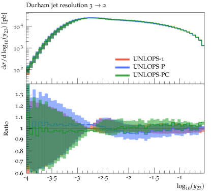
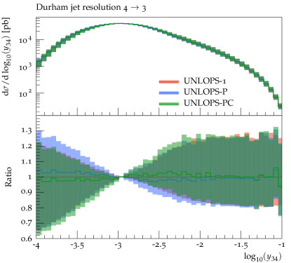
Figure 1: Differential jet separation distributions $y_{23}$ and $y_{34}$ in $e^{+}e^{-}\rightarrow\text{jets}$ at $\sqrt{s}=M_{\mathrm{Z}}$. The left distribution is described at NLO accuracy at high scales, the right at LO accuracy for all jet separations.

Figure 1 shows the differential jet separation distributions in the $3\rightarrow 2$ clustering $y_{23}$ and in the $4\rightarrow 3$ clustering $y_{34}$, with the Durham $k_{\perp}$-jet separation Catani:1991hj

$$y_{ij}=2(1-\cos\theta_{ij})\min(E_{i}^{2},E_{j}^{2})/s\,,$$ (17)

normalized with the squared CM energy $s$. The differing weighting prescriptions in the different schemes affect both the central prediction and the renormalization scale variation bands.

The $y_{23}$ jet separation distribution in fig. 1 shows that the central prediction at NLO accuracy agrees between UNLOPS-1 and UNLOPS-P at high jet separations, since the Sudakov factor is close to unity for in these regions, and no strong coupling ratios are applied in the two schemes. In the UNLOPS-PC prescription, the strong coupling ratio introduces an upward shift, by effectively evaluating the coupling at a lower scale. Going to lower scales, UNLOPS-P falls compared to UNLOPS-1, due to the Sudakov suppression. In UNLOPS-PC, the strong coupling running counteracts this effect, leading to a milder decrease. The unitary property in all schemes ensures that an increase (decrease) at high scales induces a decrease (increase) and lower scales. This leads to the observed central predictions at low separations behaving opposite to the high scale results for every scheme. High $y_{34}$ values agree for all schemes up, to statistical fluctuations, since in this region, all schemes recover the result of the UMEPS unitary merging prescription Lonnblad:2012ng . However, we observe differences at lower scales. This can be explained by the NLO precise lower multiplicity sample (here, the $e^{+}e^{-}\rightarrow 3\;\text{jet}$ NLO sample), that is modified by the different weighting prescriptions, and is showered below the merging scale, thus contributing to $y_{34}$ at small separations. Overall, the central description of jet separation observables, which are very sensitive to the merging weight prescriptions, differs by up to about 5% between the described schemes.

Scale variation bands for each merging scheme include variations of fixed-order, parton-shower and merging-reweighting origin. As opposed to renormalization scale variations in the matrix elements only, this induces larger uncertainties at small jet separations, where emissions are generated by the parton shower. For observables at LO precision, e.g. $y_{34}$ in fig. 1, variations of the scales induce a very large band, amounting to about 20% in each direction for all schemes alike. In unitary merging schemes, the subtraction of the respective jet multiplicity sample from the next-lower jet topology, turn the variation bands around, since they contribute, via showering, at low jet separations. This leads to a region with unphysically small uncertainty bands where the varied distributions cross.

Predominantly NLO precise distributions, such as $y_{23}$ in fig. 1, show smaller bands at high jet separations. In this region, renormalization scale uncertainties in the method contribute only at $\mathcal{O}(\alpha_{\mathrm{s}}^{2})$ due to NLO-precise inputs, instead of $\mathcal{O}(\alpha_{\mathrm{s}})$ otherwise. At small jet separations, the distribution is again described by parton shower emissions instead, so that a large variation is observed. At the transition, there is an unphysically small variations, as observed for LO observables.

Comparing the size of the variation bands between UNLOPS-1, UNLOPS-P and UNLOPS-PC, we note that UNLOPS-1 and UNLOPS-PC are very similar, while UNLOPS-P leads to larger scale variation bands. This suggests that the application of Sudakov suppressions alone – without taking strong coupling ratios into account – introduces an additional variation, which is partly cancelled by the coupling ratio variation in UNLOPS-PC. The Sudakov variation behaves as $1-\alpha_{\mathrm{s}}(c_{1}L^{2}+c_{2}L+c_{3})+\mathcal{O}(\alpha_{\mathrm{s}}^{2})$, while the $\alpha_{\mathrm{s}}$ ratio behaves as $1+\alpha_{\mathrm{s}}c^{\prime}L+\mathcal{O}(\alpha_{\mathrm{s}}^{2})$, where $L$ denotes a logarithmic enhancement of type $\ln{Q^{2}/p_{\perp}^{2}}$, $Q$ denotes a characteristic scale of the hard process and $p_{\perp}^{2}$ the scale of jet separation. At $\mathcal{O}(\alpha_{\mathrm{s}}^{3})$ (i.e. induced by $\mathcal{O}(\alpha_{\mathrm{s}})$ terms of the reweighting) we thus observe a partial cancellation in the single logarithmic contribution in UNLOPS-PC, which is not present in UNLOPS-P. We have found changes of similar size when setting $w_{\text{S}}=1,~{}w_{\text{NLO}}=w_{\text{LO}}$, i.e. removing the consistency condition in eq. 7 and jeopardizing the logarithmic accuracy. Thus, a very conservative uncertainty estimate that also acknowledges the potential of subleading-logarithmic mismodeling, should likely consist of the combination of the scale uncertainties of all three merging schemes.

IV.1.2 Comparison to LEP Measurements

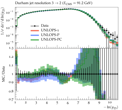
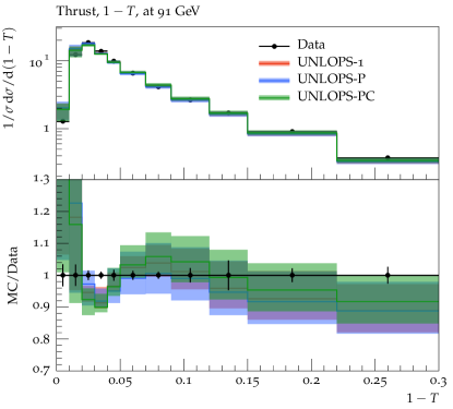
Figure 2: Renormalization scale variation bands for the differential Durham jet resolution and thrust compared for the different variations of unitary NLO multi-jet merging. Data from Heister:2003aj and Abbiendi:2004qz .

As observed above, the difference between the weighting prescriptions is rather minor, amounting to no more than about 5% for very sensitive jet separation observables. We furthermore do not observe a large difference in the description of experimentally measured data distributions. In fig. 2, we compare the thrust and Durham jet resolution to ALEPH Heister:2003aj and OPAL Abbiendi:2004qz data.

The Durham jet separation distribution is well described by all schemes, especially at large jet separations. In total, the data is compatible with the prediction of all schemes across most jet separations. Only at very low separations, where the statistical uncertainty on the data is rather large, do the prediction differ mildly from the data distribution. Overall, UNLOPS-PC agrees slightly better with the measured data distribution, compared to the other weighting schemes.

The thrust distribution

$$1-T=1-\max_{\vec{n}}\frac{\sum_{i}|\vec{n}\cdot\vec{p}_{i}|}{\sum_{i}|\vec{p}_{i}|}$$ (18)

ranges between zero for very narrow back-to-back jet configurations, corresponding to very soft “hardest” emissions, and $1/3$, corresponding to three very well separated jets. We find larger scale variations – caused by shower emissions – at low $1-T$, while high $1-T$ variations are milder. The band is in general wider than in the Durham jet separation distribution, since the thrust distribution is more sensitive to further emissions described only at LO. The agreement with data is satisfactory, with differences only at low $1-T$, where even the “hardest” emission is modeled solely by the parton shower.

In both cases, the unphysically narrow variation bands where the variations cross can potentially lead to a significant deviation from measured data. In the observables shown in fig. 2, an envelope of the result of all schemes may be used to mitigate such an effect.

IV.2 W+jets Production in Proton Proton Collisions at LHC

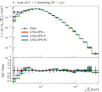
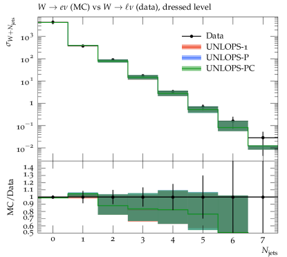
Figure 3: W + jets production at proton proton collisions with $\sqrt{s}=7$ TeV: $k_{\perp}$ splitting scale of first jet Aad:2013ueu and exclusive jet multiplicity Aad:2014qxa .

The simulation of final states in hadron collisions is typically much more involved than in lepton collisions, due to the rich structure of the composite colliding particles, as well as the larger phase-space available to the final-state particles. Thus, an assessment of uncertainties due to scale- and scheme variations in hadron colliders is necessary. In this section, we illustrate these uncertainties using $W$ + jets final states at proton-proton collisions at $\sqrt{s}=7\,\text{TeV}$. Jet observables of this process are then compared to LHC data. We use a $p_{\perp,ij}^{\mathrm{Lund}}$ merging scale definition, with value $10\,\text{GeV}$ as merging scale cut. Furthermore, we apply a NLO $K$-factor $K=\sigma_{\mathrm{NLO}}(pp\rightarrow W)/\sigma_{\mathrm{LO}}(pp\rightarrow W)$ to all leading-order input configurations that could have otherwise been reached by the $p_{\perp}$ ordered shower. Non-ordered additional jet configurations are thus interpreted as “genuine” real-emission corrections, for which a naive rate correction can be considered questionable. All results are produced using the NNPDF3.1_nlo_as_0118 PDF set Ball:2017nwa via the LHAPDF framework Buckley:2014ana .

Proton-proton collisions introduce (at least) two more sources of renormalization scale uncertainty: The treatment of running couplings in initial-state shower evolution, and in multiparton interactions. Since the latter are highly correlated with other semi- or non-perturbative parameters, we do not consider their impact in this study. Renormalization-scale and merging-scheme variations for hadronic initial states thus require only simple generalizations on top of the previous section.

Since the term in parentheses in eqs. 14$-$16 acquires PDF-dependent components, it is not obvious that the level of similarity found in $e^{+}e^{-}$ collisions is also present at hadron colliders. Figure 3 shows the weighting schemes compared to $pp\rightarrow W+\text{jets}$ data at $\sqrt{s}=7\,\text{TeV}$ for the $k_{\perp}$ $0\rightarrow 1$ clustering scale Aad:2013ueu and the exclusive jet multiplicity Aad:2014qxa . At high $\sqrt{d_{0}}$, no difference between the schemes is found. This is due to the reference renormalization scale $\mu_{\mathrm{R}}=M_{\mathrm{W}}$ chosen in the generation of matrix elements being reachable by parton showering. Thus, the differences between UNLOPS-P and UNLOPS-PC are less pronounced than in $e^{+}e^{-}$ collisions. We observe a very light suppression of UNLOPS-PC at high $\sqrt{d_{0}}$, compared to UNLOPS-P. The strong coupling ratio enhances UNLOPS-PC compared to UNLOPS-P below $M_{\mathrm{W}}$. At very low scales, the distribution is again dominated by parton shower emissions from $0$-parton states, as well as shower emissions from the integrated subtraction of the NLO 1-jet sample. The overall strong coupling ratio enhancement of the subtraction in UNLOPS-PC is consistent with the lower UNLOPS-PC result observed at low scales. Note that with the chosen PDF set, all schemes struggle to describe the low-$p_{\perp}$ region satisfactorily. This suggests that a retuning of the MPI model might be necessary when using this setup productively.

The first jet clustering scale $\sqrt{d_{0}}$ is dominated by NLO-precise contributions at high values, and thus has a very small scale variation band in that region. However, this seems to also be the case at small separation, where the parton shower, as well as MPI effects, dominate. The reason for these milder variations lies in the implementation of the shower scale variations in Pythia 8 Mrenna:2016sih : In order to avoid numerical instabilities in the reweighting procedure when approaching low scales, no shower variations are performed below a certain scale (determined by multiplication of a factor and the shower cut-off scale). In ISR, this is applied to the regularization parameter pT0Ref with default value of $2$ GeV, while in FSR, it applies to the pT0 parameter of default value $0.5$ GeV. Thus, shower variations in ISR are suppressed below transverse momentum scales of about 6 GeV. These values were chosen to limit the size of the weight fluctuations induced by the shower reweighting procedure of Mrenna:2016sih , but lead to the merging prescriptions not agreeing within their bands at low scales. Using different merging schemes thus helps to isolate phase-space regions with questionable uncertainty estimates, and a combination of scheme variations is advisable.

The right plot in fig. 3 shows the exclusive jet multiplicity of jets with $p_{\perp}>30\,\text{GeV}$ Aad:2014qxa . The 0-jet and 1-jet bins, which are described with NLO precision, are reproduced very well. Higher multiplicities, described at LO or parton-shower accuracy only, are underestimated. While the differences between UNLOPS-P and UNLOPS-PC are negligible in this observable, both schemes yield a very slightly larger exclusive 1-jet rate than UNLOPS-1. If the contribution of the term in square brackets in eqs. 14, 15 and 16 was mostly positive in the relevant region of phase space, the Sudakov factor should rather lead to a lower prediction for UNLOPS-PC and UNLOPS-P. That this is not the case suggest that the contribution is negative at least in some parts of the phase space, highlighting that there is a non-trivial interplay between the different contributions, and that rule-of-thumb reasoning should be considered with caution.

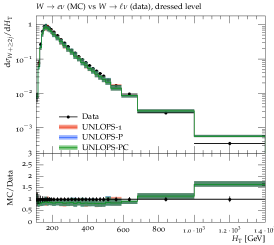
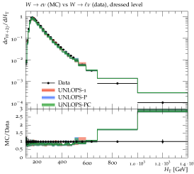
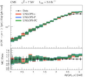
Figure 4: W + jets production at proton proton collisions with $\sqrt{s}=7$ TeV: Scalar sum of jet transverse momenta $H_{\mathrm{T}}$ for inclusive and exclusive 2 jet events Aad:2014qxa and azimuthal distance $\Delta\phi$ between hardest jet and muon Khachatryan:2014uva .

The left two plots in fig. 4 show the scalar sum of jet transverse momenta $H_{\mathrm{T}}$ for inclusive and exclusive 2-jet events. In particular distribution of $H_{\mathrm{T}}$ in exclusive 2-jet events shows a strong overshooting of the prediction, compared to the data. This is due to a mismodeling of the prediction for the transverse momenta of the first- and second-hardest jets. In inclusive 2 jet events, this effect is milder due to an underestimate of subleading jet transverse momenta, which conspires with the former effect to yield a less pronounced effect. Appropriate scale choices for unordered jet event topologies Fischer:2017yja or the inclusion of electro-weak histories Schalicke:2005nv ; Christiansen:2015jpa have been inferred to improve this situation. The new NLO merging prescriptions proposed in this study do not improve this mismodeling of data. Finally, the right plot in fig. 4 shows the azimuthal distance between the hardest jet and the muon in leptonic $W$ signatures. No significant differences between the schemes is observed, suggesting that the correlation between QCD- and electroweak parts of the events are insensitive to the scheme variation.

The observables discussed here serve as an illustrative example of the effects of scale and scheme variations in unitary NLO merging. Similar effects can be seen in other observables. More observables, processes and energies can be studied with the implementation made available in a future release of Pythia 8.3.

V Summary and Outlook

Event generator uncertainties are one of the main obstacles to precision measurements in collider experiments. This is particularly obvious when event generators are used as an accurate model of large backgrounds to high-energy signal processes with low rate appearing in the tails of Standard-Model-dominated observables. To describe such backgrounds, precise NLO merged event generator calculations are needed. Variations of perturbative parameters in such calculations should give a good indication of the overall precision of the predictions. However, since NLO merged calculations include fixed-order as well as all-order effects, and combine multiple calculations in an intricate manner, it is not completely obvious how a realistic perturbative uncertainty should be assessed. In this article, we have presented steps towards this goal, and in particular focused on the interplay between renormalization scale choices and the very definition of the merging scheme at higher orders. These enter at the same order, such that it is important to quantify their individual impact, as well as their correlation. For this purpose, we extended the unitarized NLO merging prescription in Pythia 8 to accommodate renormalization scale variations (as a combined framework encompassing correlated variations of fixed-order, parton-shower and merging components) and merging scheme changes. For the latter, we have introduced two extensions of the UNLOPS method, which were motivated by different interpretations of dressing process-dependent NLO corrections with the all-order effects of soft and collinear radiation. The implementation will be publicly available in a future release of the Pythia 8.3 event generator.

The renormalization-scale and merging-scheme variations were used to estimate the perturbative uncertainty of illustrative observables in electron-positron and proton-proton collisions. Overall, the estimate is as expected: The uncertainty is small in regions that are primarily sensitive to the NLO fixed-order components of the of the calculation, and large in regions dominated by parton showering. The renormalization scale uncertainty bands of different merging schemes largely overlap. In transition regions between calculations of different jet multiplicity, the difference between (the central result of) the schemes can be larger than scale variations, due to the latter being artificially small due to unitarity requirements. Some visible differences between the merging schemes, in size similar to scale uncertainties, can also remain in regions sensitive to very well-separated jets. This is mainly related to a different definition of the functional form of the argument of the running coupling at higher orders, which persists even in those phase space regions. Thus, a joint scale- and scheme- variation may be considered a more reliable uncertainty estimate.

The current study should be regarded as an initial step in the assessment of uncertainties in unitarized NLO merging schemes. We have focused on a subset of variations for which a minimization of contamination by statistical fluctuations in the event generation is possible through a reweighting procedure. It would be very valuable to extend this property also to other sources of uncertainty, such as consistent combined factorization-scale and shower starting-scale variations, changes in cut-off of parton-shower evolution, and changes in the merging scale definition and value. These would require an extensive redesign of the parton-shower algorithm. More insight into the effect of using different PDF parametrizations would also be valuable, but is complicated by the strong correlation with other semi- or non-perturbative components of the event generator – which is commonly held fixed after event generator tuning. Nevertheless, we believe that making the developments presented in the current study available within the Pythia 8 event generator will already allow also non-developers to perform more systematic studies of Standard-Model background uncertainties.

VI Acknowledgments

We would like to thank Peter Skands for discussions and encouragement at an early stage in the project, and Malin Sjödahl for collaboration at an early stage, and for continuous feedback. We also thank Ioannis Tsinikos for careful reading and useful comments on the manuscript. This work has received funding from the European Union’s Horizon 2020 research and innovation programme as part of the Marie Skłodowska-Curie Innovative Training Network MCnetITN3 (grant agreement no. 722104).

Appendix A Implementation Details

A.1 Merging Weight Variation

For completeness, we describe some details of the implementation of scale variations, especially for the $\mathcal{O}(\alpha_{\mathrm{s}})$ contribution.

We generate the matrix element samples with a fixed renormalization scale. At leading order, we do not use scale variations in the matrix element samples, since $\alpha_{\mathrm{s}}$ variations can simply be implemented as strong coupling ratios in Pythia based on the jet multiplicity of the event.

The all order weights are calculated as described above. For leading order samples, the strong coupling ratio has the central scale in the denominator, to be consistent with no variations in the leading order matrix element samples. Emission probability variations are generated from weight variations in the parton shower. The PDF ratio, MPI weights and the K factor are not varied.

The expanded weights to $\mathcal{O}(\alpha_{\mathrm{s}})$, which are only applied to leading order matrix element input, can be written as

$$B_{n}(\mu_{\mathrm{R}})\left(\frac{\alpha_{\mathrm{s}}(k\mu_{\mathrm{R}})}{\alpha_{\mathrm{s}}(\mu_{\mathrm{R}})}\right)^{n}\left(1+\frac{\alpha_{\mathrm{s}}(k\mu_{\mathrm{R}})}{\alpha_{\mathrm{s}}(\mu_{\mathrm{R}})}(\text{First term in $\alpha_{\mathrm{s}}(\mu_{\mathrm{R}})$ expansion of weight factors})+\{K\}_{\alpha_{\mathrm{s}}(\mu_{\mathrm{R}})}\right)\,,$$ (19)

with jet multiplicity $n$. The first order contribution to the strong coupling ratio is $\alpha_{\mathrm{s}}(k\mu_{\mathrm{R}})b_{0}/(2\pi)0.5\log(\mu_{\mathrm{R}}^{2}/p_{\perp}^{2})$. The variation in the logarithm cancels since it is applied to both the renormalization scale and the shower scale. For other weight components, only the $\alpha_{\mathrm{s}}$ coefficient is varied. The $K$ factor is not varied.

A.2 $e^{+}e^{-}$ Jet Cut

The $p_{\perp}^{\mathrm{Lund}}$ cut we employ as merging scale cut is not available for NLO matrix elements in MG5_aMC. Instead, a sufficiently inclusive jet $k_{\perp}$ cut can be used to regularize collinear divergences, and the $p_{\perp}^{\mathrm{Lund}}$ cut is then applied in Pythia 8. To make sure that this alternative $k_{\perp}$ cut is not stronger than $p_{\perp}^{\mathrm{Lund}}$ for specific configurations, the $k_{\perp}$ value is usually chosen much smaller than the desired merging cut, leading to a lower efficiency.

For electron positron collisions, a Durham $k_{\perp}$ jet cut Catani:1991hj , denoted as $d_{ij}$, can be used to regularize the $+1\,\text{jet}$ NLO matrix elements with the same value as the Lund $p_{\perp}$ Sjostrand:2004ef merging scale. The requirement for this to be allowed is $d_{ij}\geq p_{\perp,ij}^{\mathrm{Lund}}$ such that a cut on $d_{ij}$ is more inclusive than a $p_{\perp}^{\mathrm{Lund}}$ cut. The Lund shower $p_{\perp}$ is given by

$$p_{\perp,ij}^{\mathrm{Lund}}=z(1-z)q^{2}=\frac{E_{i}E_{j}}{(E_{i}+E_{j})^{2}}(m_{i}^{2}+m_{j}^{2}+2(E_{i}E_{j}-|\vec{p}_{i}||\vec{p}_{j}|\cos\theta_{ij}))\,.$$ (20)

Here we use the angle $\theta_{ij}$ between partons $i$ and $j$ and the energy fractions $z$ and $1-z$ as employed by the Pythia $p_{\perp}$ shower. If we generate events with zero quark masses, we find

$$p_{\perp,ij}^{\mathrm{Lund}} =\frac{2E_{i}^{2}E_{j}^{2}}{(E_{i}+E_{j})^{2}}(1-\cos\theta_{ij})=\frac{2\min(E_{i}^{2},E_{j}^{2})\max(E_{i}^{2},E_{j}^{2})}{(\min(E_{i},E_{j})+\max(E_{i},E_{j}))^{2}}(1-\cos\theta_{ij})$$ (21)

$$\leq\frac{2\min(E_{i}^{2},E_{j}^{2})\max(E_{i}^{2},E_{j}^{2})}{(\max(E_{i},E_{j}))^{2}}(1-\cos\theta_{ij})=2\min(E_{i}^{2},E_{j}^{2})(1-\cos\theta_{ij})=d_{ij}\,,$$ (22)

which justifies the efficient jet $d_{ij}$ cut on the generated $+1\,\text{jet}$ NLO matrix element samples. However, the above is only true for the first emission: The energy ratios in the Lund $p_{\perp}$ measure are defined in the dipole center of momentum frame, while the energies in the Durham clustering are taken in the whole event center of momentum frame. For the first emission, these two are identical. For further NLO jet corrections, which we do not employ here, and for proton proton collisions, a more conservative cut must be applied.

References

- (1) A. Buckley et al., Phys. Rept. 504, 145 (2011), 1101.2599.
- (2) T. Sjöstrand, S. Mrenna, and P. Z. Skands, JHEP 05, 026 (2006), hep-ph/0603175.
- (3) T. Sjöstrand et al., Comput. Phys. Commun. 191, 159 (2015), 1410.3012.
- (4) J. Bellm, G. Nail, S. Plätzer, P. Schichtel, and A. Siódmok, Eur. Phys. J. C76, 665 (2016), 1605.01338.
- (5) K. Cormier, S. Plätzer, C. Reuschle, P. Richardson, and S. Webster, Eur. Phys. J. C79, 915 (2019), 1810.06493.
- (6) E. Bothmann, M. Schönherr, and S. Schumann, Eur. Phys. J. C76, 590 (2016), 1606.08753.
- (7) M. Schönherr, PoS CORFU2017, 110 (2018), 1804.10643.
- (8) M. Rubin, G. P. Salam, and S. Sapeta, JHEP 09, 084 (2010), 1006.2144.
- (9) L. Lönnblad and S. Prestel, JHEP 02, 094 (2013), 1211.4827.
- (10) L. Lönnblad and S. Prestel, JHEP 03, 166 (2013), 1211.7278.
- (11) S. Plätzer, JHEP 08, 114 (2013), 1211.5467.
- (12) J. Bellm, S. Gieseke, and S. Plätzer, Eur. Phys. J. C78, 244 (2018), 1705.06700.
- (13) S. Hoeche, F. Krauss, M. Schönherr, and F. Siegert, JHEP 04, 027 (2013), 1207.5030.
- (14) J. C. Collins and D. E. Soper, Nucl. Phys. B197, 446 (1982).
- (15) J. C. Collins, D. E. Soper, and G. F. Sterman, Nucl. Phys. B250, 199 (1985).
- (16) J. C. Collins and D. E. Soper, Nucl. Phys. B193, 381 (1981), [Erratum: Nucl. Phys.B213,545(1983)].
- (17) S. Catani and M. Grazzini, Nucl. Phys. B845, 297 (2011), 1011.3918.
- (18) L. Lönnblad, JHEP 05, 046 (2002), hep-ph/0112284.
- (19) L. Lönnblad and S. Prestel, JHEP 03, 019 (2012), 1109.4829.
- (20) S. Mrenna and P. Skands, Phys. Rev. D94, 074005 (2016), 1605.08352.
- (21) S. Höche, Y. Li, and S. Prestel, Phys. Rev. D91, 074015 (2015), 1405.3607.
- (22) D. Amati, R. Petronzio, and G. Veneziano, Nucl. Phys. B146, 29 (1978).
- (23) J. Alwall et al., JHEP 07, 079 (2014), 1405.0301.
- (24) A. Buckley et al., Comput. Phys. Commun. 184, 2803 (2013), 1003.0694.
- (25) S. Catani, Y. L. Dokshitzer, M. Olsson, G. Turnock, and B. R. Webber, Phys. Lett. B269, 432 (1991).
- (26) ALEPH, A. Heister et al., Eur. Phys. J. C35, 457 (2004).
- (27) OPAL, G. Abbiendi et al., Eur. Phys. J. C40, 287 (2005), hep-ex/0503051.
- (28) ATLAS, G. Aad et al., Eur. Phys. J. C73, 2432 (2013), 1302.1415.
- (29) ATLAS, G. Aad et al., Eur. Phys. J. C75, 82 (2015), 1409.8639.
- (30) NNPDF, R. D. Ball et al., Eur. Phys. J. C77, 663 (2017), 1706.00428.
- (31) A. Buckley et al., Eur. Phys. J. C75, 132 (2015), 1412.7420.
- (32) CMS, V. Khachatryan et al., Phys. Lett. B741, 12 (2015), 1406.7533.
- (33) N. Fischer and S. Prestel, Eur. Phys. J. C77, 601 (2017), 1706.06218.
- (34) A. Schalicke and F. Krauss, JHEP 07, 018 (2005), hep-ph/0503281.
- (35) J. R. Christiansen and S. Prestel, Eur. Phys. J. C76, 39 (2016), 1510.01517.
- (36) T. Sjöstrand and P. Z. Skands, Eur. Phys. J. C39, 129 (2005), hep-ph/0408302.