Spatially quasi-periodic water waves of infinite depth

Abstract.

We formulate the two-dimensional gravity-capillary water wave equations in a spatially quasi-periodic setting and present a numerical study of solutions of the initial value problem. We propose a Fourier pseudo-spectral discretization of the equations of motion in which one-dimensional quasi-periodic functions are represented by two-dimensional periodic functions on a torus. We adopt a conformal mapping formulation and employ a quasi-periodic version of the Hilbert transform to determine the normal velocity of the free surface. Two methods of time-stepping the initial value problem are proposed, an explicit Runge-Kutta (ERK) method and an exponential time-differencing (ETD) scheme. The ETD approach makes use of the small-scale decomposition to eliminate stiffness due to surface tension. We perform a convergence study to compare the accuracy and efficiency of the methods on a traveling wave test problem. We also present an example of a periodic wave profile containing vertical tangent lines that is set in motion with a quasi-periodic velocity potential. As time evolves, each wave peak evolves differently, and only some of them overturn. Beyond water waves, we argue that spatial quasi-periodicity is a natural setting to study the dynamics of linear and nonlinear waves, offering a third option to the usual modeling assumption that solutions either evolve on a periodic domain or decay at infinity.

1. Introduction

Linear and nonlinear wave equations are generally studied under the assumption that the solution is spatially periodic or decays to zero at infinity [49]. Beginning with Berenger [15], a great deal of effort has been devoted to developing perfectly matched layer (PML) techniques for imposing absorbing boundary conditions over a finite computational domain to simulate wave propagation problems on unbounded domains. However, in many situations, assuming the waves decay to zero at infinity is not a realistic model. For example, a large body of water such as the ocean is often covered in surface waves in every direction over vast distances. But assuming spatial periodicity may limit one’s ability to observe interesting dynamics. In this paper, we formulate the initial value problem of the surface water wave equations in a spatially quasi-periodic setting, design numerical algorithms to compute such waves, and study their properties.

Since the pioneering work of Benjamin and Feir [13] and Zakharov [78], it has been recognized that water waves exhibit interesting nonlinear interactions between component waves of different wavelength. For example, in oceanography, modulational instabilities of periodic wavetrains introduce perturbations that lead to spatially quasi-periodic dynamics and are believed to be one of the mechanisms responsible for the formation of rogue waves [62, 61, 1]. These instabilities have been studied extensively using a variety of techniques, summarized below, including linearization using Bloch stability theory, evolving the nonlinear equations on a larger periodic domain, developing coupled weakly nonlinear models, and solving weakly nonlinear models via the inverse scattering transform. However, it has not been known how to formulate or compute fully nonlinear water waves in a spatially quasi-periodic setting. We show that a conformal mapping formulation of the water wave equations, introduced by Dyachenko et al. [34] and further developed by many authors [35, 27, 32, 79, 50, 56, 71, 70, 36, 68], extends nicely to this setting via a quasi-periodic generalization of the Hilbert transform. Currently our method is limited to two-dimensional fluids, but we formulate the equations of motion and discuss computational challenges of 3D quasi-periodic water waves in Appendix D.

The Bloch stability approach can be carried out by linearizing the full water wave equations about a traveling Stokes wave [51, 53, 52, 30, 67, 74] or within a weakly nonlinear model such as the nonlinear Schrödinger (NLS) equation [14, 78]. A major drawback is that unstable modes grow exponentially forever and eventually leave the realm of validity of the linearization. Osborne et. al. [62] have observed that if nonlinear effects are taken into account in this scenario, the perturbation often exhibits Fermi-Pasta-Ulam recurrence [17]. They solve a 2+1-dimensional NLS equation on a domain that is 10 times larger than the wavelength of the carrier wave and look for rogue-wave formation and recurrence over long simulation times. Similarly, Bryant and Stiassnie [25] study recurrence using both a weakly nonlinear model (Zakharov’s equation) and the full water wave equations in the context of standing water waves when the wavelength of the subharmonic perturbation is 9 times that of the unperturbed standing wave. The main drawback of this approach is that the larger periodic computational domain must be an integer multiple of both the base wave and the perturbation, which requires that the ratio of their wavelengths be a rational number with a small numerator and denominator. We propose a method below that allows for more general perturbations and plan to investigate the long-time nonlinear dynamics of unstable subharmonic perturbations of traveling and standing waves in future work.

An alternative approach that does not require rationally related wave numbers is to model the interaction of two periodic wavetrains as a coupled weakly nonlinear system. This is particularly useful for studying the interaction between oblique waves on the surface of a three-dimensional fluid. For example, Bridges and Laine-Pearson studied coupled NLS equations [22] and extended the theory to analyze the stability of short-crested waves [23]. More recently, Ablowitz and Horikis [1] showed that some propagation angles enhance the number and amplitude of rogue wave events in a coupled NLS water wave model.

Some weakly nonlinear models are completely integrable and can be studied using the inverse scattering transform (IST) [2]. Osborne et. al. discuss IST results for the 1+1-dimensional NLS equation in the context of rogue waves in [62]. Other equations such as the Korteweg-deVries and Benjamin-Ono equations are meant to model wave dynamics in shallow water [2] and internal waves in a stratified fluid [60], respectively. Solving these equations using the inverse scattering transform [2] leads to infinite hierarchies of exact spatio-temporal quasi-periodic solutions [41, 31].

In these and other examples involving weakly nonlinear theory, it is natural to seek analogous quasi-periodic solutions of the Euler equations in regimes where the model equations are intended to be accurate. It is also of interest to search for new regimes and behavior not predicted by model water wave equations. Even within weakly nonlinear theory, except for the exact quasi-periodic solutions obtained via the IST, spatial quasi-periodicity has only been approximated by embedding in a larger periodic domain or by introducing coupling terms between two or more single-mode NLS equations. The framework we propose below for water waves, which involves representing quasi-periodic functions as periodic functions on a higher dimensional torus and using a spectral method to solve a torus version of the equations of motion, could also be used to find true quasi-periodic solutions of weakly nonlinear equations without introducing systems of coupled equations.

Only recently have quasi-periodic dynamics of water waves been studied mathematically. Berti and Montalto [19] and Baldi et. al. [12] used Nash-Moser theory to prove the existence of small-amplitude temporally quasi-periodic gravity-capillary standing waves. With different assumptions on the form of solutions, Berti et. al. [18] have proved the existence of time quasi-periodic gravity-capillary waves with constant vorticity while Feola and Giuliani [39] have proved the existence of time quasi-periodic irrotational gravity waves. New families of relative-periodic [73] and traveling-standing [75] water wave solutions have been computed by Wilkening. As with [19, 12, 18, 39], these solutions are quasi-periodic in time rather than space.

Another motivation for studying spatially quasi-periodic water waves is the work of Wilton [77], who observed that a resonance can occur that causes Stokes’ regular perturbation expansion for traveling water waves to break down [7, 5, 69, 67, 6]. Suppose $k_{1}$ and $k_{2}$ are both roots of the dispersion relation for linearized water waves of infinite depth,

(1.1) $$c^{2}=gk^{-1}+\tau k.$$

Here the gravitational acceleration $g$, wave speed $c$, and surface tension $\tau$ are held constant when solving for the wave numbers $k_{1}$ and $k_{2}$. If $k_{2}=Kk_{1}$ with $K\geq 2$ an integer, the $K^{\text{th}}$ harmonic will enter a modified Stokes expansion for traveling waves of wavelength $2\pi/k_{1}$ at order $\varepsilon^{\text{max(K-2,1)}}$ instead of $\varepsilon^{K}$, where $\varepsilon$ is the expansion coefficient of the fundamental mode. This resonance occurs because the two waves travel at the same speed under the linearized water wave equations. Bridges and Dias [21] consider a generalization in which the wave numbers $k_{1}$ and $k_{2}$ are irrationally related. They use a spatial Hamiltonian structure to construct weakly nonlinear approximations of spatially quasi-periodic traveling gravity-capillary waves for two special cases: deep water and shallow water. This inspired us to develop a conformal mapping framework for computing spatially quasi-periodic, fully nonlinear traveling gravity-capillary waves, which is the topic of the companion paper [76].

We show in [76] that these spatially quasi-periodic traveling waves come in two-parameter families in which the amplitudes of the base modes with wave numbers $k_{1}$ and $k_{2}$ serve as bifurcation parameters. The wave speed and surface tension depend nonlinearly on these parameters as well. Akers et al. [6] have proved existence of similar two-parameter families of traveling waves for the case of a two-fluid hydro-elastic interface. They develop an integral equation formulation of the equations governing traveling hydro-elastic waves such that the linearization about any state is a compact perturbation of the identity and use global bifurcation theory to establish existence and uniqueness results. They show that the nullspace of the linearized operator about the flat rest state has dimension one or two, and is two if and only if the non-dimensionalized wave numbers $k_{1}<k_{2}$ that travel with a given speed are integers. When they are integers, Akers et al. distinguish resonant and non-resonant cases depending on whether $k_{2}/k_{1}$ is an integer. The non-resonant case leads to a smooth two-parameter family of traveling waves with wave speed and surface tension depending nonlinearly on the amplitude parameters. This is the case most analogous to the spatially quasi-periodic traveling waves that we compute in [76].

The present paper focuses on the more general spatially quasi-periodic initial value problem, which we use to validate the traveling wave computations of [76] and explore new dynamic phenomena. In recent years, conformal mapping methods have proved useful for studying two-dimensional traveling [27, 56, 71, 37] and time-dependent [34, 35, 32, 79, 50, 56, 36, 68] water waves with periodic boundary conditions. We introduce a Hilbert transform for quasi-periodic functions to compute the normal velocity and maintain a conformal parametrization of the free surface. This leads to a numerical method to compute the time evolution of solutions of the Euler equations from arbitrary quasi-periodic initial data. Following the definitions in [57, 38], we represent a general quasi-periodic function $u(\alpha)$ in one dimension by a periodic function $\tilde{u}(\boldsymbol{\alpha})$ on a $d$-dimensional torus, i.e. $u(\alpha)=\tilde{u}(\boldsymbol{k}\alpha)$ for $\alpha\in\mathbb{R}$, where $\boldsymbol{k}=(k_{1},\dots,k_{d})$. The $k_{i}$ are assumed to be linearly independent over the integers. We take these basic wave numbers $k_{i}$ and the initial conditions on the torus as given, focusing on the $d=2$ case. This leaves open the important question of how best to measure a one-dimensional wave profile or velocity potential and identify its quasi-periods and corresponding torus function.

We present two variants of the numerical method, one in a high-order explicit Runge-Kutta framework and one in an exponential time-differencing (ETD) framework. The former is suitable for the case of zero or small surface tension while the latter makes use of the small-scale decomposition [45, 46] to eliminate stiffness due to surface tension. The conformal mapping method has not been implemented in an ETD framework before, even for periodic boundary conditions. We present a convergence study of the methods as well as a large-scale computation of a quasi-periodic wave in which some of the wave crests overturn when evolved forward in time while others do not. Due to the torus representation of solutions, there are infinitely many wave crests and no two of them evolve in exactly the same way. The computation involves over 33 million degrees of freedom evolved over 5400 time steps to maintain double-precision accuracy.

We include four appendices that cover various technical aspects of this work. In Appendix A, we prove a theorem establishing sufficient conditions for an analytic function $z(w)$ to map the lower half-plane topologically onto a semi-infinite region bounded above by a parametrized curve and for $1/|z_{w}|$ to be uniformly bounded. In Appendix B, we study families of quasi-periodic solutions obtained by introducing phases in the reconstruction formula for extracting 1D quasi-periodic functions from periodic functions on a torus. This enables us to prove that if all the solutions in the family are single-valued and have no vertical tangent lines, the solutions are also quasi-periodic in the original graph-based formulation of the Euler equations. We also present a simple procedure for computing the change of variables from the conformal representation to the graph representation. This appears to be a new result even for periodic boundary conditions. In Appendix C we provide details on how to implement the equations of motion in an exponential time-differencing framework to avoid stepsize limitations due to stiffness caused by surface tension. And in Appendix D, we discuss the equations of motion for spatially quasi-periodic water waves in three dimensions and outline possible alternatives to the conformal mapping approach.

2. Mathematical Formulation

In this section, we review the governing equations for gravity-capillary waves in both physical space and conformal space. We then extend the conformal mapping framework to allow for spatially quasi-periodic solutions. For simplicity, we initially assume the wave profile $\eta(x,t)$ remains single-valued. This assumption is relaxed when discussing the conformal formulation, and an example of a wave in which some of the peaks overturn as time advances is presented in Section 4.2.

2.1. Governing Equations in Physical Space

Gravity-capillary waves of infinite depth are governed by the two-dimensional free-surface Euler equations [78, 29]

(2.1) $$\eta(x,0)=\eta_{0}(x),\qquad\varphi(x,0)=\varphi_{0}(x),\qquad t=0,\quad x\in\mathbb{R},$$

(2.2) $$\Phi_{xx}+\Phi_{yy} =0,\qquad-\infty<y<\eta(x,t),$$

$$\Phi_{y} \to 0,\qquad y\to-\infty,$$

$$\Phi =\varphi,\qquad y=\eta(x,t),$$

(2.3) $$\eta_{t}=\Phi_{y}-\eta_{x}\Phi_{x},\qquad y=\eta(x,t),$$

(2.4) $$\varphi_{t}=\Phi_{y}\eta_{t}-\frac{1}{2}\Phi_{x}^{2}-\frac{1}{2}\Phi_{y}^{2}-g\eta+\tau\frac{\eta_{xx}}{(1+\eta_{x}^{2})^{3/2}}+C(t),\qquad y=\eta(x,t),$$

where $x$ is the horizontal coordinate, $y$ is the vertical coordinate, $t$ is the time, $\Phi(x,y,t)$ is the velocity potential in the fluid, $\eta(x,t)$ is the free surface elevation,

(2.5) $$\varphi(x,t)=\Phi(x,\eta(x,t),t)$$

is the boundary value of the velocity potential on the free surface, $g$ is the vertical acceleration due to gravity and $\tau$ is the coefficient of surface tension. Following [78, 29], only the surface variables $\eta$ and $\varphi$ are evolved in time; the velocity potential $\Phi$ in the bulk fluid is reconstructed from $\eta$ and $\varphi$ by solving (2.2), which causes the problem to be nonlocal. The function $C(t)$ in the Bernoulli condition (2.4) is an arbitrary integration constant that is allowed to depend on time but not space. When the domain is periodic or quasi-periodic, one can choose $C(t)$ so that the mean value of $\varphi(x,t)$ remains constant in time, where the mean is defined as $\lim_{a\rightarrow\infty}\frac{1}{2a}\int_{-a}^{a}\varphi(x,t)\,dx$.

2.2. The Quasi-Periodic Hilbert Transform

We find that a conformal mapping representation of the free surface greatly simplifies the solution of the Laplace equation for the velocity potential in the quasi-periodic setting. In this section, we establish the properties of the Hilbert transform that will be needed to study quasi-periodic water waves in a conformal mapping framework.

As defined in [57, 38], a quasi-periodic, real analytic function $u(\alpha)$ is a function of the form

(2.6) $$u(\alpha)=\tilde{u}(\boldsymbol{k}\alpha),\qquad\tilde{u}(\boldsymbol{\alpha})=\sum_{\boldsymbol{j}\in\mathbb{Z}^{d}}\hat{u}_{\boldsymbol{j}}e^{i\langle\boldsymbol{j},\,\boldsymbol{\alpha}\rangle},\qquad\alpha\in\mathbb{R},\;\;\boldsymbol{\alpha},\boldsymbol{k}\in\mathbb{R}^{d},$$

where $\langle\cdot,\,\cdot\rangle$ denotes the standard inner product in $\mathbb{R}^{d}$ and $\tilde{u}$ is a periodic, real analytic function defined on the $d$-dimensional torus

(2.7) $$\mathbb{T}^{d}:=\mathbb{R}^{d}\big{/}(2\pi\mathbb{Z})^{d}.$$

Entries of the vector $\boldsymbol{k}$ are called the basic wave numbers (or basic frequencies) of $u$ and are required to be linearly independent over $\mathbb{Z}$. If $\boldsymbol{k}$ is given, one can reconstruct the Fourier coefficients $\hat{u}_{\boldsymbol{j}}$ from $u$ via

(2.8) $$\hat{u}_{\boldsymbol{j}}=\lim_{a\to\infty}\frac{1}{2a}\int_{-a}^{a}u(\alpha)e^{-i\langle\boldsymbol{j},\boldsymbol{k}\rangle\alpha}d\alpha,\qquad\boldsymbol{j}\in\mathbb{Z}^{d}.$$

A similar averaging formula holds for functions in the more general class of almost periodic functions [57, 20, 40, 9, 43], which is the closure with respect to uniform convergence on $\mathbb{R}$ of the set of trigonometric polynomials $p(x)=\sum_{n=1}^{N}c_{n}e^{i\kappa_{n}x}$. Before taking limits to obtain the closure, this set includes polynomials of any degree and there is no restriction on the real numbers $\kappa_{n}$. Within the framework of almost periodic functions, one obtains quasi-periodic functions if one assumes the $\kappa_{n}$ in the approximating polynomials are integer linear combinations of a fixed, finite set of basic wave numbers $k_{1},\dots,k_{d}$.

We have not attempted to formulate the water wave problem in the full generality of almost periodic functions, and instead assume the basic wave numbers are given and the torus representation (2.6) is available. Thus, the average over $\mathbb{R}$ on the right-hand side of (2.8) can be replaced by the simpler Fourier coefficient formula

(2.9) $$\hat{u}_{\boldsymbol{j}}=\frac{1}{(2\pi)^{d}}\int_{\mathbb{T}^{d}}\tilde{u}(\boldsymbol{\alpha})e^{-i\langle\boldsymbol{j},\boldsymbol{\alpha}\rangle}\,d\alpha_{1}\cdots\,d\alpha_{d}.$$

Our assumption that $\tilde{u}(\boldsymbol{\alpha})$ is real analytic is equivalent to the conditions that $\hat{u}_{-\boldsymbol{j}}=\overline{\hat{u}_{\boldsymbol{j}}}$ for $\boldsymbol{j}\in\mathbb{Z}^{d}$ and there exist positive numbers $M$ and $\sigma$ such that $|\hat{u}_{\boldsymbol{j}}|\leq Me^{-\sigma\|\boldsymbol{j}\|}$, i.e. the Fourier modes $\hat{u}_{\boldsymbol{j}}$ decay exponentially as $\|\boldsymbol{j}\|\rightarrow\infty$. This is proved e.g. in Lemma 5.6 of [24].

Next we define the projection operators $P$ and $P_{0}$ that act on $u$ and $\tilde{u}$ via

(2.10) $$P=\operatorname{id}-P_{0},\qquad P_{0}[u]=P_{0}[\tilde{u}]=\hat{u}_{\boldsymbol{0}}=\frac{1}{(2\pi)^{d}}\int_{\mathbb{T}^{d}}\tilde{u}(\boldsymbol{\alpha})\,d\alpha_{1}\cdots\,d\alpha_{d}.$$

Note that $P$ projects onto the space of zero-mean functions while $P_{0}$ returns the mean value, viewed as a constant function on $\mathbb{R}$ or $\mathbb{T}^{d}$. There are two versions of $P$ and $P_{0}$, one acting on quasi-periodic functions defined on $\mathbb{R}$ and one acting on torus functions defined on $\mathbb{T}^{d}$.

Given $u(\alpha)$ as in (2.6), the most general bounded analytic function $f(w)$ in the lower half-plane whose real part agrees with $u$ on the real axis has the form

(2.11) $$f(w)=\hat{u}_{\boldsymbol{0}}+i\hat{v}_{\boldsymbol{0}}+\sum_{\langle\boldsymbol{j},\boldsymbol{k}\rangle<0}2\hat{u}_{\boldsymbol{j}}e^{i\langle\boldsymbol{j},\boldsymbol{k}\rangle w},\qquad(w=\alpha+i\beta\,,\;\beta\leq 0)$$

where $\hat{v}_{\boldsymbol{0}}\in\mathbb{R}$ and the sum is over all $\boldsymbol{j}\in\mathbb{Z}^{d}$ satisfying $\langle\boldsymbol{j},\boldsymbol{k}\rangle<0$. The imaginary part of $f(z)$ on the real axis is given by

(2.12) $$v(\alpha)=\tilde{v}(\boldsymbol{k}\alpha),\qquad\tilde{v}(\boldsymbol{\alpha})=\sum_{\boldsymbol{j}\in\mathbb{Z}^{d}}\hat{v}_{\boldsymbol{j}}e^{i\langle\boldsymbol{j},\boldsymbol{\alpha}\rangle},\qquad\hat{v}_{\boldsymbol{j}}=i\operatorname{sgn}(\langle\boldsymbol{j},\boldsymbol{k}\rangle)\hat{u}_{\boldsymbol{j}},\quad(\boldsymbol{j}\neq 0)$$

where $\operatorname{sgn}(q)\in\{1,0,-1\}$ depending on whether $q>0$, $q=0$ or $q<0$, respectively. Similarly, given $v(\alpha)$ and requiring $(\operatorname{Im}f)|_{\mathbb{R}}=v$ yields (2.11) with $\hat{u}_{\boldsymbol{j}}$ replaced by $i\hat{v}_{\boldsymbol{j}}$. We introduce a quasi-periodic Hilbert transform to compute $v$ from $u$ or $u$ from $v$,

(2.13) $$v=\hat{v}_{\boldsymbol{0}}-H[u],\qquad\quad u=\hat{u}_{\boldsymbol{0}}+H[v],$$

where the constant $\hat{v}_{\boldsymbol{0}}=P_{0}[v]$ or $\hat{u}_{\boldsymbol{0}}=P_{0}[u]$ is a free parameter when computing $v$ or $u$, respectively. $H$ returns the “zero-mean” solution, i.e. $P_{0}H[u]=0$. Uniqueness of the bounded extension from $u$ or $v$ to $f$ up to the additive constant $i\hat{v}_{\boldsymbol{0}}$ or $\hat{u}_{\boldsymbol{0}}$ follows from two well-known results: the only bounded solution of the Laplace equation on a half-space satisfying homogeneous Dirichlet boundary conditions is identically zero [11], and the harmonic conjugate of the zero function on a connected domain is constant.

Definition 2.1.

The Hilbert transform of a quasi-periodic, analytic function $u(\alpha)$ of the form (2.6) is defined to be

(2.14) $$H[u](\alpha)=\sum\limits_{\boldsymbol{j}\in\mathbb{Z}^{d}}(-i)\operatorname{sgn}(\langle\boldsymbol{j},\,\boldsymbol{k}\rangle)\hat{u}_{\boldsymbol{j}}e^{i\langle\boldsymbol{j},\,\boldsymbol{k}\rangle\alpha}.$$

This agrees with the standard definition [37] of the Hilbert transform as a Cauchy principal value integral:

(2.15) $$H[u](\alpha)=\frac{1}{\pi}\operatorname{PV}\int_{-\infty}^{\infty}\frac{u(\xi)}{\alpha-\xi}\,d\xi.$$

Indeed, it is easy to show that for functions of the form $u(\alpha)=e^{i\rho\alpha}$ with $\rho$ real, the integral in (2.15) gives $H[u](\alpha)=-i\operatorname{sgn}(\rho)e^{i\rho\alpha}$. For extensions to the upper half-plane, the sum in (2.11) is over $\langle\boldsymbol{j},\boldsymbol{k}\rangle>0$, the last formula in (2.12) becomes $\hat{v}_{\boldsymbol{j}}=-i\operatorname{sgn}(\langle\boldsymbol{j},\boldsymbol{k}\rangle)\hat{u}_{\boldsymbol{j}}$, and the signs in front of $H[u]$ and $H[v]$ in (2.13) are reversed.

Remark 2.2.

As with $P$ and $P_{0}$, there is an analogous operator on $L^{2}(\mathbb{T}^{d})$ such that $H[u](\alpha)=H[\tilde{u}](\boldsymbol{k}\alpha)$. The formula is

(2.16) $$H[\tilde{u}](\boldsymbol{\alpha})=\sum\limits_{\boldsymbol{j}\in\mathbb{Z}^{d}}(-i)\operatorname{sgn}(\langle\boldsymbol{j},\,\boldsymbol{k}\rangle)\hat{u}_{\boldsymbol{j}}e^{i\langle\boldsymbol{j},\,\boldsymbol{\alpha}\rangle}.$$

If necessary for clarity, one can also write $H_{\boldsymbol{k}}[\tilde{u}]$ to emphasize the dependence of $H$ on $\boldsymbol{k}$. $H$ commutes with the shift operator $S_{\boldsymbol{\theta}}[\tilde{u}](\boldsymbol{\alpha})=\tilde{u}(\boldsymbol{\alpha}+\boldsymbol{\theta})$, so if $\tilde{v}=\hat{v}_{\boldsymbol{0}}-H[\tilde{u}]$ and $\hat{u}_{\boldsymbol{0}}=P_{0}[\tilde{u}]$, then $v(\alpha;\boldsymbol{\theta})=\tilde{v}(\boldsymbol{k}\alpha+\boldsymbol{\theta})$ is related to $u(\alpha;\boldsymbol{\theta})=\tilde{u}(\boldsymbol{k}\alpha+\boldsymbol{\theta})$ by (2.13). Also, if $f(z)$ in (2.11) is the bounded analytic extension of $(u+iv)(\alpha)=\tilde{u}(\boldsymbol{k}\alpha)+i\tilde{v}(\boldsymbol{k}\alpha)$ to the lower half-plane, we have

(2.17) $$f(w)=\tilde{f}(\boldsymbol{k}\alpha,\beta),\qquad(w=\alpha+i\beta\,,\;\beta\leq 0),$$

where $\tilde{f}(\boldsymbol{\alpha},\beta)=\hat{u}_{\boldsymbol{0}}+i\hat{v}_{\boldsymbol{0}}+\sum_{\langle\boldsymbol{j},\boldsymbol{k}\rangle<0}2[\hat{u}_{\boldsymbol{j}}e^{-\langle\boldsymbol{j},\boldsymbol{k}\rangle\beta}]e^{i\langle\boldsymbol{j},\boldsymbol{\alpha}\rangle}$ is periodic in $\boldsymbol{\alpha}$ for fixed $\beta\leq 0$. The bounded analytic extension of $[u(\alpha;\boldsymbol{\theta})+iv(\alpha;\boldsymbol{\theta})]$ to the lower half-plane is then given by $f(\alpha+i\beta;\boldsymbol{\theta})=\tilde{f}(\boldsymbol{k}\alpha+\boldsymbol{\theta},\beta)$.

2.3. The Conformal Mapping

We consider a time dependent conformal mapping that maps the conformal domain

(2.18) $$\mathbb{C}^{-}=\{\alpha+i\beta\,:\,\alpha\in\mathbb{R},\,\beta<0\}$$

to the fluid domain

(2.19) $$\Omega(t)=\{x+iy\,:\,x\in\mathbb{R},\,y<\eta(x,t)\}.$$

This conformal mapping, denoted by $z(w,t)$, is assumed to extend continuously to $\overline{\mathbb{C}^{-}}$ and maps the real line $\beta=0$ to the free surface

(2.20) $$\Gamma(t)=\{x+iy\,:\,y=\eta(x,t)\}.$$

We express $z(w,t)$ as

(2.21) $$z(w,t)=x(w,t)+iy(w,t),\qquad\quad(w=\alpha+i\beta).$$

We also introduce the notation $\zeta=z|_{\beta=0}$, $\xi=x|_{\beta=0}$ and $\eta=y|_{\beta=0}$ so that the free surface is parametrized by

(2.22) $$\zeta(\alpha,t)=\xi(\alpha,t)+i\eta(\alpha,t),\qquad\quad(\alpha\in\mathbb{R}).$$

This allows us to denote a generic field point in the physical fluid by $z=x+iy$ while simultaneously discussing points $\zeta=\xi+i\eta$ on the free surface. To avoid ambiguity, we will henceforth denote the free surface elevation function from the previous section by $\eta^{\text{phys}}(x,t)$. Thus,

(2.23) $$\eta(\alpha,t)=\eta^{\text{phys}}(\xi(\alpha,t),t),\qquad\eta_{\alpha}=\eta^{\text{phys}}_{x}\xi_{\alpha},\qquad\eta_{t}=\eta^{\text{phys}}_{x}\xi_{t}+\eta^{\text{phys}}_{t}.$$

The parametrization (2.22) is more general than (2.23) in that it allows for overturning waves. In deriving the equations of motion for $\zeta(\alpha,t)$ and $\varphi(\alpha,t)$ in Section 2.5 below, we will indicate the modifications necessary to handle the case of overturning waves. In particular, as discussed in Appendix A, $\Gamma(t)$ is defined in this case as the image of $\zeta(\cdot,t)$, which is assumed to be injective on $\mathbb{R}$, and $\Omega(t)$ can be obtained from $\Gamma(t)$ using the Jordan curve theorem.

The conformal map is required to remain a bounded distance from the identity map in the lower half-plane. Specifically, we require that

(2.24) $$|z(w,t)-w|\leq M(t)\quad\qquad(w=\alpha+i\beta\,,\;\beta\leq 0),$$

where $M(t)$ is a uniform bound that could vary in time. The Cauchy integral formula implies that $|z_{w}-1|\leq M(t)/|\beta|$, so at any fixed time,

(2.25) $$z_{w}\rightarrow 1\quad\text{ as }\quad\beta\to-\infty.$$

Our goal is to investigate the case when the free surface is quasi-periodic in $\alpha$. This differs from conformal mappings discussed in [54, 34, 32, 79, 50, 56], where it is assumed to be periodic.

In the present work, $\eta$ is assumed to have two spatial quasi-periods, i.e. at any time it has the form (2.6) with $d=2$ and $\boldsymbol{k}=[k_{1},k_{2}]^{T}$. Since $k_{1}$ and $k_{2}$ are irrationally related, we assume without loss of generality that $k_{1}=1$ and $k_{2}=k$, where $k$ is irrational:

(2.26) $$\eta(\alpha,t)=\tilde{\eta}(\alpha,k\alpha,t),\qquad\tilde{\eta}(\alpha_{1},\alpha_{2},t)=\sum_{j_{1},j_{2}\in\mathbb{Z}}\hat{\eta}_{j_{1},j_{2}}(t)e^{i(j_{1}\alpha_{1}+j_{2}\alpha_{2})}.$$

Here $\hat{\eta}_{-j_{1},-j_{2}}(t)=\overline{\hat{\eta}_{j_{1},j_{2}}(t)}$ since $\tilde{\eta}(\alpha_{1},\alpha_{2},t)$ is real-valued. Since $w\mapsto[z(w,t)-w]$ is bounded and analytic on $\mathbb{C}^{-}$ and its imaginary part agrees with $\eta$ on the real axis, there is a real number $x_{0}$ (possibly depending on time) such that

(2.27) $$\xi(\alpha,t)=\alpha+x_{0}(t)+H[\eta](\alpha,t).$$

Using (2.25) and  $\operatorname{Im}[z_{w}|_{\beta=0}]=\eta_{\alpha}$  or differentiating (2.27) gives

(2.28) $$\xi_{\alpha}(\alpha,t)=1+H[\eta_{\alpha}](\alpha,t).$$

We use a tilde to denote the periodic functions on the torus that correspond to the quasi-periodic parts of $\xi$, $\zeta$ and $z$,

(2.29) $$\begin{gathered}\xi(\alpha,t)=\alpha+\tilde{\xi}(\alpha,k\alpha,t),\qquad\zeta(\alpha,t)=\alpha+\tilde{\zeta}(\alpha,k\alpha,t),\\ z(\alpha+i\beta,t)=\left(\alpha+i\beta\right)+\tilde{z}(\alpha,k\alpha,\beta,t),\qquad(\beta\leq 0).\end{gathered}$$

Specifically, $\tilde{\xi}=x_{0}(t)+H[\tilde{\eta}]$, $\tilde{\zeta}=\tilde{\xi}+i\tilde{\eta}$, and

(2.30) $$\tilde{z}(\alpha_{1},\alpha_{2},\beta,t)=x_{0}(t)+i\hat{\eta}_{0,0}(t)+\sum_{j_{1}+j_{2}k<0}\left(2i\hat{\eta}_{j_{1},j_{2}}(t)e^{-(j_{1}+j_{2}k)\beta}\right)e^{i(j_{1}\alpha_{1}+j_{2}\alpha_{2})}.$$

While the mean surface height remains constant in physical space, $\hat{\eta}_{0,0}(t)$ generally varies in time. Since the modes $\hat{\eta}_{j_{1},j_{2}}$ are assumed to decay exponentially, there is a uniform bound $M(t)$ such that $|\tilde{z}(\alpha_{1},\alpha_{2},\beta,t)|\leq M(t)$ for $(\alpha_{1},\alpha_{2})\in\mathbb{T}^{2}$ and $\beta\leq 0$. In Appendix A we show that as long as the free surface $\zeta(\alpha,t)$ does not self-intersect at a given time $t$, the mapping $w\mapsto z(w,t)$ is an analytic isomorphism of the lower half-plane onto the fluid region.

2.4. The Complex Velocity Potential

Let $\Phi^{\text{phys}}(x,y,t)$ denote the velocity potential in physical space from Section 2.1 above and let $W^{\text{phys}}(x+iy,t)=\Phi^{\text{phys}}(x,y,t)+i\Psi^{\text{phys}}(x,y,t)$ be the complex velocity potential, where $\Psi^{\text{phys}}$ is the stream function. Using the conformal mapping (2.21), we pull back these functions to the lower half-plane and define

$$W(w,t)=\Phi(\alpha,\beta,t)+i\Psi(\alpha,\beta,t)=W^{\text{phys}}(z(w,t),t),\qquad\quad(w=\alpha+i\beta).$$

We also define $\varphi=\Phi|_{\beta=0}$ and $\psi=\Psi|_{\beta=0}$ and use (2.2) and (2.23) to obtain

(2.31) $$\varphi(\alpha,t)=\varphi^{\text{phys}}(\xi(\alpha,t),t),\qquad\psi(\alpha,t)=\psi^{\text{phys}}(\xi(\alpha,t),t),$$

where $\psi^{\text{phys}}(x,t)=\Psi^{\text{phys}}(x,\eta^{\text{phys}}(x,t),t)$. We assume $\varphi$ is quasi-periodic with the same quasi-periods as $\eta$,

$$\varphi(\alpha,t)=\tilde{\varphi}(\alpha,k\alpha,t),\qquad\tilde{\varphi}(\alpha_{1},\alpha_{2},t)=\sum_{j_{1},j_{2}\in\mathbb{Z}}\hat{\varphi}_{j_{1},j_{2}}(t)e^{i(j_{1}\alpha_{1}+j_{2}\alpha_{2})}.$$

The fluid velocity $\nabla\Phi^{\text{phys}}(x,y,t)$ is assumed to decay to zero as $y\rightarrow-\infty$ (since we work in the lab frame). From (2.25) and the chain rule (see (2.33) below), $dW/dw\rightarrow 0$ as $\beta\to-\infty$. Thus, $\psi_{\alpha}=-H[\varphi_{\alpha}]$. Writing this as $\partial_{\alpha}[\psi+H\varphi]=0$, we conclude that

(2.32) $$\psi(\alpha,t)=-H[\varphi](\alpha,t).$$

Here we have set the integration constant to zero and assumed $P_{0}[\varphi]=\hat{\varphi}_{0,0}(t)=0$ and $P_{0}[\psi]=\hat{\psi}_{0,0}(t)=0$, which is allowed since $\Phi$ and $\Psi$ can be modified by additive constants (or functions of time only) without affecting the fluid motion.

2.5. Governing Equations in Conformal Space

Following [34, 27, 79, 50, 70, 68], we present a derivation of the equations of motion for surface water waves in a conformal mapping formulation, modified as needed to handle quasi-periodic solutions. We also justify the assumption that $z_{t}/z_{\alpha}$ remains bounded in the lower half-plane, which we have not seen discussed previously in the literature.

From the chain rule,

(2.33) $$\frac{dW}{dw}=\frac{dW^{\text{phys}}}{dz}\cdot\frac{dz}{dw}\qquad\Rightarrow\qquad\Phi^{\text{phys}}_{x}+i\Psi^{\text{phys}}_{x}=\frac{\Phi_{\alpha}+i\Psi_{\alpha}}{x_{\alpha}+iy_{\alpha}}.$$

Evaluating (2.33) on the free surface gives

(2.34) $$\Phi^{\text{phys}}_{x}=\frac{\varphi_{\alpha}\xi_{\alpha}+\psi_{\alpha}\eta_{\alpha}}{J},\qquad\Phi^{\text{phys}}_{y}=-\Psi^{\text{phys}}_{x}=\frac{\varphi_{\alpha}\eta_{\alpha}-\psi_{\alpha}\xi_{\alpha}}{J},\qquad J=\xi_{\alpha}^{2}+\eta_{\alpha}^{2}.$$

Using (2.23) and (2.34) in (2.3) and multiplying by $\xi_{\alpha}$, we obtain

(2.35) $$\eta_{t}\xi_{\alpha}-\xi_{t}\eta_{\alpha}=-\psi_{\alpha}.$$

This states that the normal velocity of the free surface is equal to the normal velocity of the fluid, $\boldsymbol{\hat{n}}\cdot(\xi_{t},\eta_{t})=\boldsymbol{\hat{n}}\cdot\nabla\Phi^{\text{phys}}$, where $\boldsymbol{\hat{n}}=(-\eta_{\alpha},\xi_{\alpha})/\sqrt{J}$. This can also be obtained by tracking a fluid particle $x_{p}(t)+iy_{p}(t)=\zeta(\alpha_{p}(t),t)$ on the free surface. We have $\dot{x}_{p}=\xi_{\alpha}\dot{\alpha}_{p}+\xi_{t}=\Phi^{\text{phys}}_{x}$ and $\dot{y}_{p}=\eta_{\alpha}\dot{\alpha}_{p}+\eta_{t}=\Phi^{\text{phys}}_{y}$, which leads to (2.35) after eliminating $\dot{\alpha}_{p}$. This argument does not assume the free surface is a graph, i.e. (2.35) is also valid for overturning waves.

Next we define a new function,

(2.36) $$q:=\frac{\zeta_{t}}{\zeta_{\alpha}}=\frac{(\xi_{t}\xi_{\alpha}+\eta_{t}\eta_{\alpha})+i(\eta_{t}\xi_{\alpha}-\xi_{t}\eta_{\alpha})}{J}=\frac{(\xi_{t}\xi_{\alpha}+\eta_{t}\eta_{\alpha})-i\psi_{\alpha}}{J}.$$

Since $q$ is quasi-periodic in $\alpha$ and extends analytically to the lower half-plane via $z_{t}/z_{\alpha}$, the real and imaginary part of $q$ can be related by the Hilbert transform. Here we have assumed that $z_{t}/z_{\alpha}$ is bounded, which will be justified below. Thus,

(2.37) $$\frac{\xi_{t}\xi_{\alpha}+\eta_{t}\eta_{\alpha}}{J}=-H\left[\frac{\psi_{\alpha}}{J}\right]+C_{1},$$

where $C_{1}$ is an arbitrary integration constant that may depend on time but not space. Let $\boldsymbol{\hat{s}}=(\xi_{\alpha},\eta_{\alpha})/\sqrt{J}$ denote the unit tangent vector to the curve. Equation (2.37) prescribes the tangential velocity  $\boldsymbol{\hat{s}}\cdot(\xi_{t},\eta_{t})$  of points on the curve in terms of the normal velocity in order to maintain a conformal parametrization. Note that the tangent velocity of the curve differs from that of the underlying fluid particles. This is similar in spirit to a method of Hou, Lowengrub and Shelley [45, 46], who proposed a tangential velocity that maintains a uniform parametrization of the curve (rather than a conformal one); see also [27, 68, 8, 76]. Combining (2.35) and (2.37), we obtain the kinematic boundary conditions in conformal space,

(2.38) $$\begin{pmatrix}\xi_{t}\\ \eta_{t}\end{pmatrix}=\begin{pmatrix}\xi_{\alpha}&-\eta_{\alpha}\\ \eta_{\alpha}&\xi_{\alpha}\end{pmatrix}\begin{pmatrix}-H\left[\frac{\psi_{\alpha}}{J}\right]+C_{1}\\ -\frac{\psi_{\alpha}}{J}\end{pmatrix}.$$

The right-hand side can be interpreted as complex multiplication of $z_{\alpha}$ with $z_{t}/z_{\alpha}$. Since both functions are analytic in the lower half-plane, their product is, too. Thus, $\xi_{t}$ is related to $\eta_{t}$ via the Hilbert transform (up to a constant). The constant is determined by comparing (2.27) with (2.38), which gives

(2.39) $$\frac{dx_{0}}{dt}=P_{0}\left[\xi_{\alpha}\left(-H\left[\frac{\psi_{\alpha}}{J}\right]+C_{1}\right)+\frac{\eta_{\alpha}\psi_{\alpha}}{J}\right].$$

The three most natural choices of $C_{1}$ are

(2.40) $$(a)\;\;C_{1} =0: \text{evolve $x_{0}(t)$ via (\ref{eq:x0:evol})},$$

$$(b)\;\;C_{1} =P_{0}\big{[}\xi_{\alpha}H[\psi_{\alpha}/J]-\eta_{\alpha}\psi_{\alpha}/J\big{]}: x_{0}(t)=0,$$

$$(c)\;\;C_{1} =\big{[}H[\psi_{\alpha}/J]-\eta_{\alpha}\psi_{\alpha}/(\xi_{\alpha}J)\big{]}_{\alpha=0}: \xi(0,t)=0.$$

In options ($b$) and ($c$), the evolution equation ensures that $dx_{0}/dt=0$ and $\xi_{t}(0,t)=0$, respectively; we have assumed the initial conditions satisfy $x_{0}(0)=0$ or $\xi(0,0)=0$, respectively. Option ($c$) amounts to setting $x_{0}(t)=-H[\eta](0,t)$ in (2.27). This arguably leads to the most natural parametrization, but would have a problem if the vertical part of an overturning wave crosses $\alpha=0$. Indeed, such a crossing would lead to $\xi_{\alpha}(0,t)=0$ at some time $t$ in the denominator of (2.40c). We recommend option ($b$) in this scenario.

Remark 2.3.

In infinite depth as considered here, if $\tilde{f}$ and $\tilde{g}$ are torus functions on $\mathbb{T}^{d}$ and $f(\alpha)=\tilde{f}(\boldsymbol{k}\alpha)$, $g(\alpha)=\tilde{g}(\boldsymbol{k}\alpha)$, the identity

(2.41) $$P_{0}\big{[}fg-(Hf)(Hg)\big{]}=\sum_{\langle\boldsymbol{j},\boldsymbol{k}\rangle=0}\hat{f}_{\boldsymbol{j}}\hat{g}_{-\boldsymbol{j}}$$

is easily proved, where the sum is over $\boldsymbol{j}\in\mathbb{Z}^{d}$ satisfying $\langle\boldsymbol{j},\boldsymbol{k}\rangle=0$. In the periodic case with $d=1$ and $\boldsymbol{k}=(1)$ or the quasi-periodic case with $\boldsymbol{k}=(k_{1},\dots,k_{d})$ and the $k_{i}$ linearly independent over the integers, the right-hand side of (2.41) is $\hat{f}_{\boldsymbol{0}}\hat{g}_{\boldsymbol{0}}$. This simplifies (2.40b) to $C_{1}=0$ and (2.39) to $dx_{0}/dt=C_{1}$, i.e. cases (a) and (b) in (2.40) coincide. However, this only works in infinite depth as the finite-depth Hilbert transform with symbol $-i\tanh\big{(}\langle\boldsymbol{j},\boldsymbol{k}\rangle h\big{)}$ does not satisfy (2.41). Here $h$ is the fluid depth in conformal space, which evolves in time to maintain constant fluid depth in physical space [50, 68]. Finite-depth quasi-periodic water waves will be investigated in future work.

Next we evaluate the Bernoulli equation  $\Phi^{\text{phys}}_{t}+\frac{1}{2}\big{|}\nabla\Phi^{\text{phys}}\big{|}^{2}+\frac{p}{\rho}+gy=C_{2}$  at the free surface to obtain an evolution equation for $\varphi(\alpha,t)$. Here $C_{2}$ is an arbitrary integration constant that may depend on time but not space. The pressure at the free surface is determined by the Laplace-Young condition, $p=p_{0}-\rho\tau\kappa$, where $\kappa$ is the curvature, $\rho\tau$ is the surface tension, and $p_{0}$ is a constant that can be absorbed into $C_{2}$ and set to zero. From (2.33) or (2.34), we know $\big{|}\nabla\Phi^{\text{phys}}\big{|}^{2}=(\varphi_{\alpha}^{2}+\psi_{\alpha}^{2})/J$ on the free surface. Finally, differentiating $\varphi(\alpha,t)=\Phi^{\text{phys}}(\xi(\alpha,t),\eta(\alpha,t),t)$ and using (2.34) and (2.38), we obtain

(2.42) $$\varphi_{t}=\underbrace{\big{(}\Phi^{\text{phys}}_{x}\,,\,\Phi^{\text{phys}}_{y}\big{)}\begin{pmatrix}\xi_{\alpha}&-\eta_{\alpha}\\ \eta_{\alpha}&\xi_{\alpha}\end{pmatrix}}_{\displaystyle\big{(}\varphi_{\alpha}\,,\,-\psi_{\alpha}\big{)}}\begin{pmatrix}-H\left[\psi_{\alpha}/J\right]+C_{1}\\ -\psi_{\alpha}/J\end{pmatrix}-\frac{\varphi_{\alpha}^{2}+\psi_{\alpha}^{2}}{2J}-g\eta+\tau\kappa+C_{2}.$$

We choose $C_{2}$ so that $P_{0}[\varphi_{t}]=0$. In conclusion, we obtain the following governing equations for spatially quasi-periodic gravity-capillary waves in conformal space

(2.43) $$\begin{gathered}\xi_{\alpha}=1+H[\eta_{\alpha}],\qquad\psi=-H[\varphi],\qquad J=\xi_{\alpha}^{2}+\eta_{\alpha}^{2},\qquad\chi=\frac{\psi_{\alpha}}{J},\\[2.0pt] \text{ choose $C_{1}$, e.g.~{}as in (\ref{eq:C1:opt}), \qquad compute\, $\displaystyle\frac{dx_{0}}{dt}$\, in (\ref{eq:x0:evol}) if necessary,}\\[2.0pt] \eta_{t}=-\eta_{\alpha}H[\chi]-\xi_{\alpha}\chi+C_{1}\eta_{\alpha},\qquad\kappa=\frac{\xi_{\alpha}\eta_{\alpha\alpha}-\eta_{\alpha}\xi_{\alpha\alpha}}{J^{3/2}},\\[-4.0pt] \varphi_{t}=P\bigg{[}\frac{\psi_{\alpha}^{2}-\varphi_{\alpha}^{2}}{2J}-\varphi_{\alpha}H[\chi]+C_{1}\varphi_{\alpha}-g\eta+\tau\kappa\bigg{]}.\end{gathered}$$

Note that these equations govern the evolution of $x_{0}$, $\eta$ and $\varphi$, which determine the state of the system. The functions $\xi$, $\psi$, $J$, $\chi$ and $\kappa$ are determined at any moment by $x_{0}$, $\eta$ and $\varphi$ through the auxiliary equations in (2.43). We emphasize that $C_{1}$ can be chosen arbitrarily as long as $dx_{0}/dt$ satisfies (2.39). The special cases (2.40b) and (2.40c) lead to nice formulas for $x_{0}(t)$ without having to evolve (2.39) numerically. An alternative approach was proposed by Li et al. [50], who set $C_{1}=0$ (by not introducing it) and avoid writing down a differential equation for $x_{0}(t)$ by instead solving both the $\xi_{t}$ and $\eta_{t}$ equations in (2.38).

In deriving (2.43) from (2.35) and (2.42), we had to assume $z_{t}/z_{\alpha}$ remains bounded in the lower half-plane. Conditions that ensure the boundedness of $1/z_{\alpha}$ are given in Appendix A. We note that $z_{t}/z_{\alpha}$ is automatically bounded in the converse direction, where (2.35) and (2.42) are derived from (2.43). In more detail, when solving (2.43), $z_{t}/z_{\alpha}$ is constructed first, before $z_{t}$, as the bounded extension of the quasi-periodic function with imaginary part $(-\psi_{\alpha}/J)$ to the lower half-plane. Equation (2.38) then defines $z_{t}$ as the product of this function by $z_{\alpha}$, which is also bounded since $\xi_{\alpha}=1+H[\eta_{\alpha}]$. Thus, the first component of each side of (2.38) is related to the corresponding second component by the Hilbert transform, up to a constant. Since the second components are equal (i.e. the $\eta_{t}$ equation holds), the $\xi_{t}$ equation also holds — the constants are accounted for by (2.39). Left-multiplying (2.38) by the row vector $[-\eta_{\alpha},\xi_{\alpha}]$ gives the kinematic condition (2.35), as required.

Equations (2.43) break down if $J$ becomes zero somewhere on the curve. Such a singularity would arise, for example, if the wave profile were to form a corner in finite time. To our knowledge, it remains an open question whether the free-surface Euler equations can form such a corner.

Often we wish to verify that a given curve $\zeta(\alpha,t)=\xi(\alpha,t)+i\eta(\alpha,t)$ and velocity potential $\varphi(\alpha,t)$ satisfy the conformal version of the water wave equations. We say that $(\zeta,\varphi)$ satisfy (2.43) if $\xi$ and $\eta$ remain conformally related via (2.27), which determines $x_{0}(t)$, and if $x_{0}$, $\eta$ and $\varphi$ satisfy (2.43) with $C_{1}(t)$ obtained from (2.39) using $P_{0}[\xi_{\alpha}]=1$. As noted above, these equations imply the kinematic condition (2.35) and Bernoulli equation (2.42). If necessary, one should replace the given $\varphi(\alpha,t)$ by $P[\varphi(\cdot,t)]$ before checking that (2.43) is satisfied.

Remark 2.4.

Equations (2.43) can be interpreted as an evolution equation for the functions $\tilde{\zeta}(\alpha_{1},\alpha_{2},t)$ and $\tilde{\varphi}(\alpha_{1},\alpha_{2},t)$ on the torus $\mathbb{T}^{2}$. The $\alpha$-derivatives are replaced by the directional derivatives $(\partial_{\alpha_{1}}+k\partial_{\alpha_{2}})$, which we still denote by a subscript $\alpha$, e.g. $\tilde{\eta}_{\alpha}=(\partial_{\alpha_{1}}+k\partial_{\alpha_{2}})\tilde{\eta}$, and, as noted in Remark 2.2 above, the Hilbert transform becomes a two-dimensional Fourier multiplier operator with symbol $(-i)\operatorname{sgn}(j_{1}+j_{2}k)$. The pseudo-spectral method we propose in Section 3 below is based on this representation. Equation (2.40c) becomes

(2.44) $$C_{1}=\left[H\left[\frac{\tilde{\psi}_{\alpha}}{\tilde{J}}\right]-\frac{\tilde{\eta}_{\alpha}\tilde{\psi}_{\alpha}}{(1+\tilde{\xi}_{\alpha})\tilde{J}}\right]_{(\alpha_{1},\alpha_{2})=(0,0)},\qquad\quad\tilde{\xi}(0,0,t)=0,$$

where $\tilde{J}=(1+\tilde{\xi}_{\alpha})^{2}+\tilde{\eta}_{\alpha}^{2}$. Note that $\xi_{\alpha}$ in (2.43) is replaced by

(2.45) $$\widetilde{\xi_{\alpha}}=1+\tilde{\xi}_{\alpha},$$

which is the one place this notation becomes awkward. Using (2.27) and (2.29), $\tilde{\zeta}$ is completely determined by $x_{0}(t)$ and $\tilde{\eta}$, so only these have to be evolved — the formula for $\tilde{\xi}_{t}$ in (2.38) is redundant as long as (2.39) is satisfied. If both components of $\tilde{\zeta}(\alpha_{1},\alpha_{2},t)$ are given, we say that $(\tilde{\zeta},\tilde{\varphi})$ satisfy the torus version of (2.43) if there is a continuously differentiable function $x_{0}(t)$ such that $\tilde{\xi}=x_{0}(t)+H[\tilde{\eta}]$ and if $x_{0}$, $\tilde{\eta}$ and $\tilde{\varphi}$ satisfy the torus version of (2.43) with $C_{1}=dx_{0}/dt+P_{0}\big{[}(1+\tilde{\xi}_{\alpha})H[\tilde{\psi}_{\alpha}/\tilde{J}]-\tilde{\eta}_{\alpha}\tilde{\psi}_{\alpha}/\tilde{J}\big{]}$. As noted in Remark 2.3, if $k$ is irrational, one can verify that $P_{0}\left[\tilde{\xi}_{\alpha}H[\tilde{\psi}_{\alpha}/\tilde{J}]-\tilde{\eta}_{\alpha}\tilde{\psi}_{\alpha}/\tilde{J}\right]=0$, hence $dx_{0}/dt=C_{1}$.

We show in Appendix B that solving the torus version of (2.43) yields a three-parameter family of one-dimensional solutions of the form

(2.46) $$\begin{aligned} \zeta(\alpha,t\,;\,\theta_{1},\theta_{2},\delta)&=\alpha+\delta+\tilde{\zeta}(\theta_{1}+\alpha,\theta_{2}+k\alpha,t),\\ \varphi(\alpha,t\,;\,\theta_{1},\theta_{2})&=\tilde{\varphi}(\theta_{1}+\alpha,\theta_{2}+k\alpha,t),\end{aligned}\qquad\left(\begin{aligned} \alpha\in\mathbb{R},\,t\geq 0\\ \theta_{1},\theta_{2},\delta\in\mathbb{R}\end{aligned}\right).$$

We also show that if all the waves in this family are single-valued and have no vertical tangent lines, there is a corresponding family of solutions of the Euler equations in the original graph-based formulation of (2.1)–(2.4) that are quasi-periodic in physical space. A precise statement is given in Theorem B.2 and the discussion that follows.

3. Numerical Method

In this section, we describe a pseudo-spectral time-stepping strategy for evolving water waves with spatially quasi-periodic initial conditions. The evolution equations (2.43) for $\eta$ and $\varphi$ are nonlinear and involve computing derivatives, antiderivatives and Hilbert transforms of quasi-periodic functions. Let $f$ denote one of these functions (e.g. $\eta$, $\varphi$ or $\chi$) and let $\tilde{f}$ denote the corresponding periodic function on the torus,

(3.1) $$f(\alpha)=\tilde{f}(\alpha,k\alpha),\qquad\tilde{f}(\alpha_{1},\alpha_{2})=\sum\limits_{j_{1},j_{2}\in\mathbb{Z}}\hat{f}_{j_{1},j_{2}}e^{i(j_{1}\alpha_{1}+j_{2}k\alpha_{2})},\qquad(\alpha_{1},\alpha_{2})\in\mathbb{T}^{2}.$$

The functions $f_{\alpha}$ and $H[f]$ then correspond to

(3.2) $$\begin{gathered}\widetilde{f_{\alpha}}(\alpha_{1},\alpha_{2})=\sum\limits_{j_{1},j_{2}\in\mathbb{Z}}i(j_{1}+j_{2}k)\hat{f}_{j_{1},j_{2}}e^{i(j_{1}\alpha_{1}+j_{2}\alpha_{2})},\\ \widetilde{H[f]}(\alpha_{1},\alpha_{2})=\sum\limits_{j_{1},j_{2}\in\mathbb{Z}}(-i)\text{sgn}(j_{1}+j_{2}k)\hat{f}_{j_{1},j_{2}}e^{i(j_{1}\alpha_{1}+j_{2}\alpha_{2})}.\end{gathered}$$

We propose a pseudo-spectral method in which each such $f$ that arises in the formulas (2.43) is represented by the values of $\tilde{f}$ at $M_{1}\times M_{2}$ equidistant gridpoints on the torus $\mathbb{T}^{2}$,

(3.3) $$\tilde{f}_{m_{1},m_{2}}=\tilde{f}(2\pi m_{1}/M_{1}\,,\,2\pi m_{2}/M_{2}),\qquad\quad(0\leq m_{1}<M_{1}\,,\,0\leq m_{2}<M_{2}).$$

We visualize a $90^{\circ}$ rotation between the matrix $\tilde{F}$ holding the entries $\tilde{f}_{m_{1},m_{2}}$ and the collocation points in the torus. The columns of the matrix correspond to horizontal slices of gridpoints while the rows of the matrix correspond to vertical slices indexed from bottom to top. The nonlinear operations in (2.43) consist of products, powers and division; they are carried out pointwise on the grid. Derivatives and the Hilbert transform are computed in Fourier space via (3.2). To plot the solution, we also need to compute an antiderivative to get $\xi$ from $f=\xi_{\alpha}$. This involves dividing $\hat{f}_{j_{1},j_{2}}$ by $i(j_{1}+j_{2}k)$ when $(j_{1},j_{2})\neq(0,0)$ and adjusting the $(0,0)$ mode to obtain $\xi(0,t)=0$.

Since the functions $f$ that arise in the computation are real-valued, we use the real-to-complex (‘r2c’) version of the two-dimensional discrete Fourier transform. The ‘r2c’ transform of a one-dimensional array of length $M$ (assumed even) is given by

(3.4) $$\{g_{m}\}_{m=0}^{M-1}\quad\mapsto\quad\{\hat{g}_{j}\}_{j=0}^{M/2}\quad,\quad\hat{g}_{j}=\frac{1}{M}\sum_{m=0}^{M-1}g_{m}e^{-2\pi ijm/M}.$$

In practice, the $\hat{g}_{j}$ are computed simultaneously in $O(M\log M)$ time rather than by this formula. The fully complex (‘c2c’) transform of this (real) data would give additional values $\hat{g}_{j}$ with $M/2+1\leq j\leq M-1$. These extra entries are actually aliased values of negative-index modes; they are redundant due to $\hat{g}_{j}=\hat{g}_{j-M}=\overline{\hat{g}_{M-j}}$. Since the imaginary components of $\hat{g}_{0}$ and $\hat{g}_{M/2}$ are zero, the number of real degrees of freedom on both sides of (3.4) is $M$. The Nyquist mode $\hat{g}_{M/2}$ requires special attention. Setting $\hat{g}_{M/2}=1$ and the other modes to zero yields $g_{m}=\cos(\pi m)=(-1)^{m}$. The derivative and Hilbert transform of this mode are taken to be zero since they would involve evaluating $\sin(M\alpha/2)$ at the gridpoints $\alpha_{m}=2\pi m/M$.

The two-dimensional ‘r2c’ transform can be computed by applying one-dimensional ‘r2c’ transforms in the $x$-direction (i.e. to the columns of $\tilde{F}$) followed by one-dimensional ‘c2c’ transforms in the $y$-direction (i.e. to the rows of $\tilde{F}$):

(3.5) $$\hat{f}_{j_{1},j_{2}}=\frac{1}{M_{2}}\sum_{m_{2}=0}^{M_{2}-1}\left(\frac{1}{M_{1}}\sum_{m_{1}=0}^{M_{1}-1}\tilde{f}_{m_{1},m_{2}}e^{-2\pi ij_{1}m_{1}/M_{1}}\right)e^{-2\pi ij_{2}m_{2}/M_{2}},\quad\left(\begin{gathered}0\leq j_{1}\leq M_{1}/2\\ -M_{2}/2<j_{2}\leq M_{2}/2\end{gathered}\right).$$

The ‘r2c’ routine in the FFTW library actually returns the index range $0\leq j_{2}<M_{2}$, but we use $\hat{f}_{j_{1},j_{2}-M_{2}}=\hat{f}_{j_{1},j_{2}}$ to de-alias the Fourier modes and map the indices $j_{2}>M_{2}/2$ to their correct negative values. The missing entries with $-M_{1}/2<j_{1}<0$ are determined implicitly by

(3.6) $$\hat{f}_{-j_{1},-j_{2}}=\overline{\hat{f}_{j_{1},j_{2}}}.$$

This imposes additional constrains on the computed Fourier modes, namely

(3.7) $$\begin{gathered}\operatorname{Im}\{\hat{f}_{0,0}\}=0,\quad\operatorname{Im}\{\hat{f}_{M_{1}/2,0}\}=0,\quad\operatorname{Im}\{\hat{f}_{0,M_{2}/2}\}=0,\quad\operatorname{Im}\{\hat{f}_{M_{1}/2,M_{2}/2}\}=0,\\ \hat{f}_{0,-j_{2}}=\overline{\hat{f}_{0,j_{2}}},\qquad\hat{f}_{M_{1}/2,-j_{2}}=\overline{\hat{f}_{M_{1}/2,j_{2}}},\qquad(1\leq j_{2}\leq M_{2}/2-1),\end{gathered}$$

where we also used $\hat{f}_{-M_{1}/2,j_{2}}=\hat{f}_{M_{1}/2,j_{2}}$. This reduces the number of real degrees of freedom in the complex $(M_{1}/2+1)\times M_{2}$ array of Fourier modes to $M_{1}M_{2}$. When computing $f_{\alpha}$ and $H[f]$ via (3.2), the Nyquist modes with $j_{1}=M_{1}/2$ or $j_{2}=M_{2}/2$ are set to zero. Otherwise the formulas (3.2) respect the constraints (3.7) and the ‘c2r’ transform reconstructs real-valued functions $\widetilde{f_{\alpha}}$ and $\widetilde{H[f]}$ from their Fourier modes.

The evolution equations (2.43) are not stiff when the surface tension parameter is small or vanishes, but become moderately stiff for larger values of $\tau$. We find that the 5th and 8th order explicit Runge-Kutta methods of Dormand and Prince [42] work well for smaller values of $\tau$, and exponential time-differencing (ETD) methods [28, 47, 16, 72, 26] work well generally. This will be demonstrated in Sections 4.1 and 4.2 below. In the ETD framework, we follow the basic idea of the small-scale decomposition for removing stiffness from interfacial flows [45, 46] and write the evolution equations (2.43) in the form

(3.8) $$\begin{pmatrix}\eta_{t}\\ \varphi_{t}\end{pmatrix}=L\begin{pmatrix}\eta\\ \varphi\end{pmatrix}+\mathcal{N},\qquad L=\begin{pmatrix}0&H\partial_{\alpha}\\ -(gP-\tau\partial_{\alpha\alpha})&0\end{pmatrix},$$

where $P$ is the projection in (2.10), $H$ is the Hilbert transform in (2.14), and

(3.9) $$\mathcal{N}=\begin{pmatrix}-\eta_{\alpha}H[\chi]-\big{(}\xi_{\alpha}\chi-\psi_{\alpha}\big{)}+C_{1}\eta_{\alpha}\\ P\left[\frac{\psi_{\alpha}^{2}-\varphi_{\alpha}^{2}}{2J}-\varphi_{\alpha}H[\chi]+C_{1}\varphi_{\alpha}+\tau(\kappa-\eta_{\alpha\alpha})\right]\end{pmatrix}.$$

Note that $\mathcal{N}$ is obtained by subtracting the terms included in $L$ from (2.43). In particular, $\psi_{\alpha}$ in (3.9) is $-H\partial_{\alpha}\varphi$ from (3.8). The eigenvalues of  $L$  are  $\pm i\sqrt{|j_{1}+j_{2}k|\big{(}g+\tau(j_{1}+j_{2}k)^{2}\big{)}}$, so the leading source of stiffness is dispersive. This $3/2$ power growth rate of the eigenvalues of the leading dispersive term with respect to wave number is typical of interfacial fluid flows with surface tension [45, 46]. For stiffer problems such as the Benjamin-Ono and KdV equations, the growth rate is faster (quadratic and cubic, respectively) and it becomes essential to use a semi-implicit or exponential time-differencing scheme to avoid severe time-stepping restrictions. Here it is less critical, but still useful. Further details on how to implement (3.8) and (3.9) in the ETD framework are given in Appendix C.

In both the explicit Runge-Kutta and ETD methods, as explained above, the functions evolved in time are $\tilde{\eta}(\alpha_{1},\alpha_{2},t)$ and $\tilde{\varphi}(\alpha_{1},\alpha_{2},t)$, sampled on the uniform $M_{1}\times M_{2}$ grid covering $\mathbb{T}^{2}$. At the end of each time step, we apply a 36th order filter [44, 45] with Fourier multiplier

(3.10) $$\rho(j_{1},j_{2})=\left\{\begin{array}[]{cc}0&j_{1}=M_{1}/2\text{\, or\, }|j_{2}|=M_{2}/2,\\[3.0pt] \exp\big{(}\!-36\big{[}(2j_{1}/M_{1})^{36}+(2j_{2}/M_{2})^{36}\big{]}\big{)}&\text{otherwise.}\end{array}\right.$$

In all the computations reported below, we used the same number of gridpoints in the $\alpha_{1}$ and $\alpha_{2}$-directions, $M_{1}=M_{2}=M$. It is easy to check a-posteriori that the Fourier modes decay sufficiently (e.g. to machine precision) by the time the filter deviates appreciably from 1. If they do not, the calculation can be repeated with a larger value of $M$. This will be demonstrated in Section 4.2 below.

4. Numerical Results

In this section, we compute spatially quasi-periodic solutions of the initial value problem (2.43) with $k=1/\sqrt{2}$ and $g$ normalized to 1. First we validate the traveling wave computations of [76] and compare the accuracy and efficiency of the ERK and ETD schemes in a convergence study. We then consider more complex dynamics in which some of the wave peaks overturn.

4.1. Traveling waves

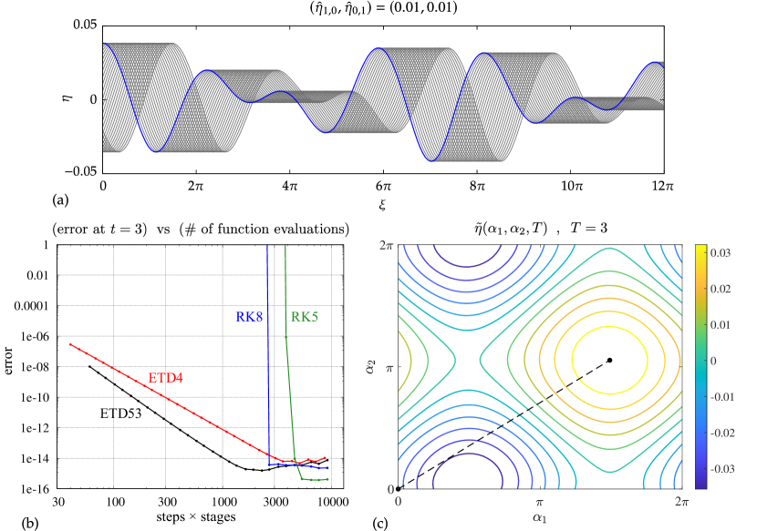
Figure 1. Time evolution of a quasi-periodic traveling water wave computed in [76] and a convergence plot comparing the accuracy and efficiency of the proposed time-stepping schemes.

Figure 1 shows the time evolution of a traveling wave computed at $t=0$ by the algorithm of [76] with amplitude parameters $\hat{\eta}_{1,0}=0.01$ and $\hat{\eta}_{0,1}=0.01$ and evolved to $t=T$ using the methods of Section 3, where $T=3$. It also shows the error at the final time $T$ for various choices of time-stepping scheme and number of time steps. In all the computations of the figure, the torus functions $\tilde{\eta}(\alpha_{1},\alpha_{2},t)$ and $\tilde{\varphi}(\alpha_{1},\alpha_{2},t)$ are evolved on an $M\times M$ mesh with $M=60$ gridpoints in each direction. Panel (a) shows snapshots of the solution in the lab frame at 30 equal time intervals of size $T/30=0.1$. Here we plotted every 30th step of the 5th order, 6 stage explicit Runge-Kutta method of Dormand and Prince [42], so the Runge-Kutta stepsize was $\Delta t=0.1/30$. The initial condition is plotted with a thick blue line, and the wave travels right at constant speed $c=1.552197$ in physical space. The solution is plotted over the representative interval $0\leq x\leq 12\pi$, though it extends in both directions to $\pm\infty$ without exactly repeating.

Panel (b) shows the error in time-stepping this traveling wave solution from $t=0$ to $t=3$ using the 5th and 8th order explicit Runge-Kutta methods of Dormand and Prince [42], the 4th order ETD scheme of Cox and Matthews [28, 47], and the 5th order ETD scheme of Whalen, Brio and Moloney [72]. These errors compare the numerical solution from time-stepping the initial condition to the exact formula of how a quasi-periodic traveling wave should evolve under (2.43) and (2.44), which is worked out in [76]. If the initial wave profile has the torus representation $\tilde{\eta}_{0}(\alpha_{1},\alpha_{2})$, we define $\tilde{\xi}_{0}=H[\tilde{\eta}_{0}]$ and $\tilde{\varphi}_{0}=c\tilde{\xi}_{0}$. By construction [76], $\tilde{\eta}_{0}$ is an even function of $\boldsymbol{\alpha}=(\alpha_{1},\alpha_{2})$, so $\tilde{\xi}_{0}$ and $\tilde{\varphi}_{0}$ are odd. The exact traveling solution is then

(4.1) $$\tilde{\eta}_{\text{exact}}(\boldsymbol{\alpha},t) =\tilde{\eta}_{0}\big{(}\boldsymbol{\alpha}-\boldsymbol{k}\alpha_{0}(t)\big{)},$$

$$\tilde{\varphi}_{\text{exact}}(\boldsymbol{\alpha},t) =\tilde{\varphi}_{0}\big{(}\boldsymbol{\alpha}-\boldsymbol{k}\alpha_{0}(t)\big{)},$$

where $\boldsymbol{k}=(1,k)$, $\alpha_{0}(t)=ct-\mathcal{A}(-\boldsymbol{k}ct,0)$ and $\mathcal{A}(\boldsymbol{x},t)$ is a periodic function on $\mathbb{T}^{2}$ defined implicitly by (B.7) below. To derive (4.1), one makes use of the change of variables formula (B.8) from physical space, where the wave speed is constant, to conformal space; see [76]. Note that the waves in (4.1) do not change shape as they move through the torus in the direction $\boldsymbol{k}$, but the traveling speed $\alpha_{0}^{\prime}(t)$ in conformal space varies in time in order to maintain $\tilde{\xi}(0,0,t)=0$ via (2.44). The error plotted in panel (b) is the discrete norm at the final time computed, $T=3$:

$$\text{err}=\sqrt{\|\tilde{\eta}-\tilde{\eta}_{\text{exact}}\|^{2}+\|\tilde{\varphi}-\tilde{\varphi}_{\text{exact}}\|^{2}},\qquad\|\tilde{\eta}\|^{2}=\frac{1}{M_{1}M_{2}}\sum_{m_{1},m_{2}}\tilde{\eta}\left(\frac{2\pi m_{1}}{M_{1}},\frac{2\pi m_{2}}{M_{2}},T\right)^{2}.$$

The surface tension in this example ($\tau=1.410902$) is high enough that once the stepsize is sufficiently small for the Runge-Kutta methods to be stable, roundoff error dominates truncation error. So the errors suddenly drop from very large values ($10^{20}$ or more) to machine precision. By contrast, the error in the ETD methods decreases steadily as the stepsize is reduced, indicating that the small-scale decomposition introduced in (3.8) is successful in removing stiffness from the equations of motion [45, 46].

A contour plot of $\tilde{\eta}(\alpha_{1},\alpha_{2},T)$ at $t=T=3$ is shown in panel (c) of Figure 1. The dashed line shows the trajectory from $t=0$ to $t=3$ of the wave crest that begins at $(0,0)$ and continues along the path $\alpha_{1}=\alpha_{0}(t),$ $\alpha_{2}=k\alpha_{0}(t)$. We use Newton’s method to solve the implicit equation (B.7) for $\mathcal{A}(\boldsymbol{x},0)$ at each point of the pseudo-spectral grid. We then use FFTW to compute the 2D Fourier representation of $\mathcal{A}(\boldsymbol{x},0)$, which can then be used to quickly evaluate the function at any point. We find that the Fourier modes of $\mathcal{A}(\boldsymbol{x},0)$ decay to machine precision on the $M\times M$ grid with $M=60$, corroborating the assertion in Theorem B.2 below that $\mathcal{A}(x_{1},x_{2},t)$ is real analytic in $x_{1}$ and $x_{2}$.

4.2. Overturning waves

Next we present a spatially quasi-periodic water wave computation in which some of the wave peaks overturn as they evolve while others do not. Conformal mapping methods have been used previously to compute overturning waves. For example, Dyachenko and Newell [36] use this approach to study whitecapping in the ocean and Wang et al. [71] use it to compute solitary and periodic overturning traveling flexural-gravity waves. The novelty of our work is the computation of a spatially quasi-periodic water wave in which every wave peak evolves differently, and only some of them overturn. Since torus functions are involved, the number of degrees of freedom is squared, leading to a large-scale computation. For simplicity, we set the surface tension parameter, $\tau$, to zero.

We first seek spatially periodic dynamics in which the initial wave profile has a vertical tangent line that overturns when evolved forward in time and flattens out when evolved backward in time. Through trial and error, we selected the following parametric curves for the initial wave profile and velocity potential of this auxiliary periodic problem:

(4.2) $$\xi_{1}(\sigma)=\sigma+\frac{3}{5}\sin\sigma-\frac{1}{5}\sin 2\sigma,\qquad\begin{aligned} \eta_{1}(\sigma)&=-(1/2)\cos(\sigma+\pi/2.5),\\ \varphi_{1}(\sigma)&=-(1/2)\cos(\sigma+\pi/4).\end{aligned}$$

Note that $\xi_{1}^{\prime}(\sigma)=0$ when $\sigma\in\pi+2\pi\mathbb{Z}$, and otherwise $\xi_{1}^{\prime}(\sigma)>0$. Thus, vertical tangent lines occur where $\xi_{1}(\sigma)\in\pi+2\pi\mathbb{Z}$ and $\eta_{1}(\sigma)=-0.5\cos(1.4\pi)=0.154508$; see Figure 2.

To convert (4.2) to a conformal parametrization, we search for $2\pi$-periodic functions $\eta_{2}(\alpha)$ and $B_{2}(\alpha)$ and a number $x_{2}$ such that

(4.3) $$\alpha+x_{2}+H\left[\eta_{2}\right](\alpha)=\xi_{1}(\alpha+B_{2}(\alpha)),\qquad\eta_{2}(\alpha)=\eta_{1}(\alpha+B_{2}(\alpha)),\qquad B_{2}(0)=0.$$

First we solve a simpler variant in which $x_{2}$ is absent and $B_{2}(0)$ is unspecified. Specifically, we solve $\alpha+H\left[\eta_{3}\right](\alpha)=\xi_{1}(\alpha+B_{3}(\alpha))$, $\eta_{3}(\alpha)=\eta_{1}(\alpha+B_{3}(\alpha))$ for $\eta_{3}(\alpha)$ and $B_{3}(\alpha)$ on a uniform grid with $M=4096$ gridpoints on $[0,2\pi)$ using Newton’s method. The Hilbert transform is computed with spectral accuracy in Fourier space. We then define $x_{2}$ as the solution of $x_{2}+B_{3}(x_{2})=0$ that is smallest in magnitude. We solve this equation by a combination of root bracketing and Newton’s method; the result is $x_{2}=0.393458$. Finally, we define $B_{2}(\alpha)=x_{2}+B_{3}(\alpha+x_{2})$ and $\eta_{2}(\alpha)=\eta_{3}(\alpha+x_{2})$, which satisfy (4.3).

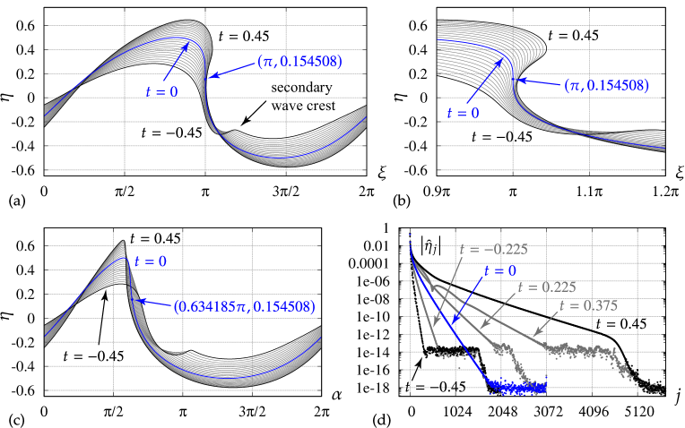
Figure 2. Time evolution of a spatially periodic water wave initialized via (4.2) and evolved forward and backward in time to $t=\pm 0.45$. Panels (a) and (b) show snapshots of the wave in physical space; panel (c) shows snapshots of $\eta(\alpha,t)$ in conformal space; and panel (d) shows snapshots of $|\hat{\eta}_{j}(t)|$ in Fourier space. The initial condition ($t=0$) is shown in blue in each plot.

As shown in Figure 2, the initial conditions $\eta_{2}(\alpha)$ and

(4.4) $$\varphi_{2}(\alpha)=\varphi_{1}(\alpha+B_{2}(\alpha))$$

have the desired property that the wave overturns when evolved forward in time and flattens out when evolved backward in time. In other words, the wave becomes less steep in the neighborhood of the initial vertical tangent line when time is reversed. However, it does not evolve backward to a flat state. Instead, a secondary wave crest forms to the right of the initial wave crest and grows in amplitude as $t$ decreases. This secondary wave crest resembles the early stages of the fluid jets that were observed by Aurther et al. [10] to form in the wave troughs when the initial condition $\eta_{0}(x)=\big{(}\frac{1}{3}\sin x+\frac{1}{6}\sin 2x+\frac{1}{3}\sin 3x)$ is evolved from rest in the graph-based formulation (2.1).

The blue markers in panels (a) and (b) of Figure 2 show the location of the vertical tangent line in physical space at $t=0$. The blue marker in panel (c) shows the corresponding point in conformal space. When the wave overturns for $t>0$ in physical space, it is because $\alpha\mapsto\xi(\alpha,t)$ no longer increases monotonically. Indeed, we see in panel (c) that $\eta(\alpha,t)$ remains single-valued as a function of the conformal variable $\alpha$ but becomes very steep. This causes the Fourier mode amplitudes in panel (d) to decay more slowly as $t$ increases. We used different mesh sizes and timesteps in the regions $0\leq t\leq 0.3$, $0.3\leq t\leq 0.45$ and $0\geq t\geq-0.45$ to maintain spectral accuracy; details are given below when discussing the quasi-periodic calculation. The drop-off in $|\hat{\eta}_{j}|$ from $10^{-14}$ to $10^{-18}$ as $j$ approaches the Nyquist frequency $M/2$ is due to the 1D version of the filter (3.10), which is applied after each timestep. Floating point errors of size $10^{-14}$ occur in the discretization of the equations of motion while errors of size $10^{-18}$ are due to having computed the inverse FFT of the filtered data to get back to real space before taking the FFT again to plot the Fourier data.

We turn the solution of this auxiliary periodic problem into a spatially quasi-periodic solution by defining initial conditions on the torus of the form

(4.5) $$\tilde{\eta}_{0}(\alpha_{1},\alpha_{2})=\eta_{2}(\alpha_{1}),\qquad\tilde{\varphi}_{0}(\alpha_{1},\alpha_{2})=\varphi_{2}(\alpha_{1})\cos(\alpha_{2}-q),$$

where $q$ is a free parameter that we choose heuristically to be $q=0.6k\pi=1.3329$ in order to make the first wave crest to the right of the origin behave similarly to the periodic 1D solution of Figure 2. (This will be explained below).

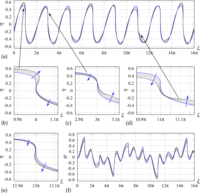
Figure 3. Snapshots in time of a spatially quasi-periodic water wave with a periodic initial wave profile with vertical tangent lines at $\xi=\pi+2\pi n$, $n\in\mathbb{Z}$. A quasi-periodic initial velocity potential causes some of the peaks to overturn for $t>0$ while others do not. Panels (a) and (f) show $\eta(\alpha,t)$ and $\varphi(\alpha,t)$ versus $\xi(\alpha,t)$ over $0\leq x\leq 16\pi$ and $0\leq t\leq T=0.225$. Panels (b)–(e) show the results of panel (a) in more detail. The blue arrows show the direction of travel of the wave at various locations.

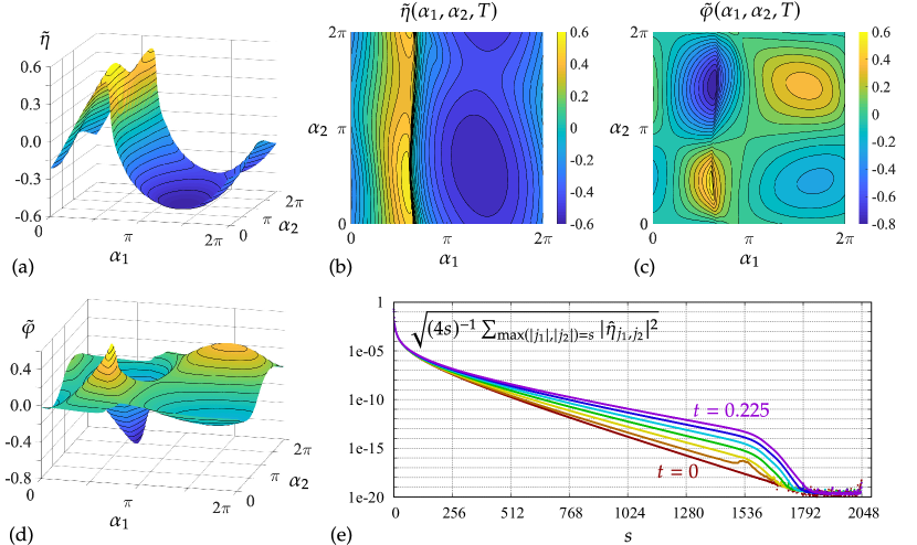
Figure 4. Surface and contour plots of the torus version of the solution plotted in Figure 3 at the final time $T=0.225$. The rapid dropoff in $\tilde{\eta}(\alpha_{1},\alpha_{2},t)$ over the window $0.6\pi\leq\alpha_{1}\leq 0.667\pi$ persists from the initial state in which $\tilde{\eta}_{0}(\alpha_{1},\alpha_{2})$ does not depend on $\alpha_{2}$. Panel (e) shows the exponential decay of Fourier modes with respect to the shell index $s$ at different times.

The results of the quasi-periodic calculation are summarized in Figures 3 and 4. Panel (a) of Figure 3 shows snapshots of the solution at $t=(\ell/6)T$ for $0\leq\ell\leq 6$ over the range $0\leq\xi(\alpha)\leq 16\pi$, where $T=0.225$. The initial wave profile, $\zeta_{0}(\alpha)=\xi_{0}(\alpha)+i\eta_{0}(\alpha)$ with $\eta_{0}(\alpha)=\tilde{\eta}_{0}(\alpha,k\alpha)$, is plotted with a thick blue line. The wave profile is plotted with a thick black line at $t=T$ and with thin grey lines at intermediate times. Panel (b) zooms in on the first wave in panel (a), which overturns as the wave crest moves up and right while the wave trough moves down and left, as indicated by the blue arrows. This is very similar (by design) to the forward evolution of the auxiliary periodic wave of Figure 2, with initial conditions $\eta_{2}(\alpha)$, $\varphi_{2}(\alpha)$. Panels (c) and (d) zoom in on two other wave crests from panel (a) that flatten out (rather than overturn) as $t$ advances from 0 to $T$. Panel (e) shows another type of behavior in which the wave overturns due to the wave trough moving down and left faster than the wave crest moves down and left. Panel (f) shows the evolution of the velocity potential $\varphi(\alpha,t)$ over $0\leq t\leq T$. Unlike $\eta_{0}(\alpha)$, the initial velocity potential $\varphi_{0}(\alpha)=\tilde{\varphi}_{0}(\alpha,k\alpha)$ is not $2\pi$-periodic due to the factor of $\cos(\alpha_{2}-q)$ in (4.5).

Panels (a) and (d) of Figure 4 show surface plots of $\tilde{\eta}(\alpha_{1},\alpha_{2},T)$ and $\tilde{\varphi}(\alpha_{1},\alpha_{2},T)$ at the final time computed, $T=0.225$. The corresponding contour plots are shown in panels (b) and (c). Initially, $\tilde{\eta}(\alpha_{1},\alpha_{2},0)$ depends only on $\alpha_{1}$; however, by $t=T$, the dependence on $\alpha_{2}$ is clearly visible. Although the waves overturn in some places when $\eta(\alpha,t)=\tilde{\eta}(\alpha,k\alpha,t)$ is plotted parametrically versus $\xi(\alpha,t)$ with $t>0$ held fixed, both $\tilde{\eta}$ and $\tilde{\varphi}$ are single-valued functions of $\alpha_{1}$ and $\alpha_{2}$ at all times. Nevertheless, throughout the evolution, $\tilde{\eta}(\alpha_{1},\alpha_{2},t)$ has a steep dropoff over a narrow range of values of $\alpha_{1}$. Initially, $\tilde{\eta}_{0}(\alpha_{1},\alpha_{2})=\eta_{2}(\alpha_{1})=\eta_{1}(\alpha_{1}+B_{2}(\alpha_{1}))$ and the rapid dropoff occurs for $\alpha_{1}$ near the solution of $\alpha_{1}+B_{2}(\alpha_{1})=\pi$ (since the vertical tangent line occurs at $\xi_{1}(\sigma)+i\eta_{1}(\sigma)$ with $\sigma=\pi$). Using Newton’s method, we find that this occurs at $\alpha_{1}=0.634185\pi$. The blue curve in panel (c) of Figure 2 gives $\eta_{2}(\alpha)$. If one zooms in on this plot, one finds that $\eta_{2}(\alpha)$ decreases rapidly by more than half its crest-to-trough height over the narrow range $0.6\pi\leq\alpha\leq 0.667\pi$. At later times, $\tilde{\eta}(\alpha_{1},\alpha_{2},t)$ continues to drop off rapidly when $\alpha_{1}$ traverses this narrow range in spite of the dependence on $\alpha_{2}$. This can be seen in panel (b) of Figure 4, where there is a high clustering of nearly vertical contour lines separating the yellow-orange region from the blue region. Over this narrow window, $\tilde{\varphi}(\alpha_{1},\alpha_{2},t)$ also varies rapidly with respect to $\alpha_{1}$.

Many gridpoints are needed to resolve these rapid variations with spectral accuracy. Although $\xi_{1}(\sigma)$, $\eta_{1}(\sigma)$ and $\varphi_{1}(\sigma)$ involve only a few nonzero Fourier modes, conformal reparametrization via (4.3) vastly increases the Fourier content of the initial condition. We used $M=6144$ gridpoints to evolve the periodic auxiliary problem of Figure 2 from $t=0$ to $t=0.3$ using the 8th order Runge-Kutta method of Dormand and Prince [42] with stepsize $\Delta t=2.08333\times 10^{-5}$. We then switched to $M=12288$ gridpoints to evolve from $t=0.3$ to $t=0.45$ with $\Delta t=7.5\times 10^{-6}$. In the reverse direction, we used $M=4096$ gridpoints to evolve from $t=0$ to $t=-0.45$ with $\Delta t=-4.6875\times 10^{-5}$. Studying the Fourier modes in panel (d) of Figure 2, it appears that 4096 gridpoints (2048 modes) are sufficient to maintain double-precision accuracy forward or backward in time to $t=\pm 0.225$. Using this as a guideline for the quasi-periodic calculation, we evolved (2.43) on a $4096\times 4096$ spatial grid using the 8th order explicit Runge-Kutta method described in Section 3. The calculation involved 5400 time steps from $t=0$ to $t=T=0.225$, which took 2.5 days on 12 threads running on a server with two 3.0 GHz Intel Xeon Gold 6136 processors. Additional threads had little effect on the running time as the FFT calculations require a lot of data movement relative to the number of floating point operations involved.

Panel (e) of Figure 4 shows the $\ell^{2}$ average of the Fourier mode amplitudes $|\hat{\eta}_{j_{1},j_{2}}|$ in each shell of indices satisfying $\max(|j_{1}|,|j_{2}|)=s$ for $1\leq s\leq 2048$. Since $\hat{\eta}_{-j_{1},-j_{2}}=\overline{\hat{\eta}_{j_{1},j_{2}}}$, we can discard half the modes and sweep through the lattice along straight lines from $(0,s)$ to $(s,s)$ to $(s,-s)$ to $(1,-s)$, which sweeps out $4s$ index pairs. (The same ordering is used to enumerate the unknowns in the nonlinear least squares method proposed in [76] to compute quasi-periodic traveling water waves.) We see in panel (e) that as time increases, the modes continue to decay at an exponential rate with respect to $s$, but the decay rate is slower at later times. The rapid dropoff in the mode amplitudes for $s\geq 1536$ is due to the Fourier filter. At the final time $t=T=0.225$, the modes still decay by 12 orders of magnitude from $s=1$ to $s=1536$, so we believe the solution is correct to 10–12 digits. A finer grid would be required to maintain this accuracy over longer times. As in Figure 2, the additional drop-off in the amplitude of Fourier modes from $s=1536$ to $s=2048$ in panel (e) is due applying the filter (3.10) to the solution after every timestep.

Beyond monitoring the decay of Fourier modes, as an additional check of accuracy, we compute the average energy, mass and momentum of the solution of Figure 4 as a function of time. The results are shown in Table 1. The formulas for $E$, $M$ and $P_{x}$ are

(4.6) $$E =\frac{1}{(2\pi)^{2}}\int_{\mathbb{T}^{2}}\bigg{[}\,\frac{1}{2}\tilde{\psi}\tilde{\varphi}_{\alpha}+\frac{1}{2}g\tilde{\eta}^{2}\big{(}1+\tilde{\xi}_{\alpha}\big{)}+\tau\left(\sqrt{\big{(}1+\tilde{\xi}_{\alpha}\big{)}^{2}+\big{(}\tilde{\eta}_{\alpha}\big{)}^{2}}-1\right)\!\bigg{]}\,d\alpha_{1}\,d\alpha_{2},$$

$$M =\frac{1}{(2\pi)^{2}}\int_{\mathbb{T}^{2}}\tilde{\eta}\big{(}1+\tilde{\xi}_{\alpha}\big{)}\,d\alpha_{1}\,d\alpha_{2},\qquad P_{x}=\frac{1}{(2\pi)^{2}}\int_{\mathbb{T}^{2}}-\tilde{\varphi}\tilde{\eta}_{\alpha}\,d\alpha_{1}\,d\alpha_{2},$$

which may be shown to be conserved quantites under the free-surface Euler equations following the derivations in [79, 33]. The only changes required for the quasi-periodic case are that derivatives and the Hilbert transform are replaced by their torus versions, and the integrals over $\mathbb{R}$ or $\mathbb{T}$ are replaced by integrals over $\mathbb{T}^{2}$. We also divide by $(2\pi)^{2}$ to obtain average values over the torus. This scaling has the advantage that $E$, $M$ and $P_{x}$ do not suddenly jump by a factor of $2\pi$ when periodic functions are viewed as quasi-periodic functions that depend on $\alpha_{1}$ only. The equations of motion are Hamiltonian [78, 33] whether or not the energy is scaled by $1/(2\pi)^{2}$ — one just has to multiply the symplectic 2-form [3] by the same factor.

The numerical results in Table 1 show that energy is conserved to a relative error of $1.5\times 10^{-13}/0.0975=1.5\times 10^{-12}$; mass is conserved to a relative error of $3.3\times 10^{-13}/0.0464=7.1\times 10^{-12}$; and momentum is conserved to an absolute error of $4.6\times 10^{-15}$ over the course of the numerical computation of Figure 4. This gives further evidence that $\tilde{\eta}$ and $\tilde{\varphi}$ are accurate to 10–12 digits. The mass being negative is an artifact of the choice of $\xi_{1}(\sigma)$ and $\eta_{1}(\sigma)$ in (4.2). While $\eta_{1}(\sigma)$ has zero mean as a function of $\sigma$, its average value with respect to $x$ is $(2\pi)^{-1}\int_{0}^{2\pi}\eta_{1}(\sigma)\xi_{1}^{\prime}(\sigma)\,d\sigma=-(3\pi/40)(\sqrt{5}-1)=-0.04635254915624$. If we had added a constant to $\tilde{\eta}$ to make $M$ zero initially, it would have remained zero up numerical errors, similar to $P_{x}$, which is initially zero since $\tilde{\eta}$ and $\tilde{\varphi}$ in (4.5) are independent of $\alpha_{2}$ except for the factor of $\cos(\alpha_{2}-q)$. The constant value of the energy would also change if a constant were added to $\tilde{\eta}$.

$$\begin{array}[]{c|c|c|r}t&E&M&P_{x}\\ \hline\cr 0.000&0.097501331570\textbf{54}&-0.046352549156\textbf{43}&1.19\times 10^{-15}\\ \hline\cr 0.025&0.097501331570\textbf{57}&-0.046352549156\textbf{23}&-2.98\times 10^{-15}\\ \hline\cr 0.050&0.097501331570\textbf{58}&-0.046352549156\textbf{21}&-1.24\times 10^{-15}\\ \hline\cr 0.075&0.097501331570\textbf{57}&-0.046352549156\textbf{19}&1.15\times 10^{-15}\\ \hline\cr 0.100&0.097501331570\textbf{59}&-0.046352549156\textbf{17}&0.43\times 10^{-15}\\ \hline\cr 0.125&0.097501331570\textbf{60}&-0.046352549156\textbf{16}&0.34\times 10^{-15}\\ \hline\cr 0.150&0.097501331570\textbf{62}&-0.046352549156\textbf{14}&4.59\times 10^{-15}\\ \hline\cr 0.175&0.097501331570\textbf{63}&-0.046352549156\textbf{13}&1.35\times 10^{-15}\\ \hline\cr 0.200&0.097501331570\textbf{64}&-0.046352549156\textbf{11}&-2.18\times 10^{-15}\\ \hline\cr 0.225&0.097501331570\textbf{69}&-0.046352549156\textbf{10}&-2.10\times 10^{-15}\\ \end{array}\vspace*{10pt}$$

Table 1. Average energy, mass and momentum of the overturning wave example of Figure 4 at the times indicated.

The rationale for setting $q=0.6k\pi$ in (4.5) is that $\cos(\alpha_{2}-q)\approx 1$ where the characteristic line $(\alpha,k\alpha)$ crosses the dropoff in the torus near $\alpha_{1}=0.6\pi$ for the first time. Locally, $\varphi_{0}(\alpha)=\tilde{\varphi}_{0}(\alpha,k\alpha)$ is close to $\varphi_{2}(\alpha)$, the initial condition of the auxiliary periodic problem, so we expect the quasi-periodic wave to evolve similarly to the periodic wave near $x=\pi$ for a short time. (Here $z=x+iy$ describes physical space). This is indeed what happens, which may be seen by comparing panel (b) of Figure 2 to panel (b) of Figure 3, keeping in mind that $t\in[-0.45,0.45]$ in the former plot and $t\in[0,0.225]$ in the latter plot. Advancing $\alpha$ from $0.6\pi$ to $10.6\pi$ causes the characteristic line $(\alpha,k\alpha)$ to cross a periodic image of the dropoff at $\alpha_{2}=10.6k\pi$, where $\cos(\alpha_{2}-q)=-0.9752\approx-1$. Locally, $\varphi_{0}(\alpha)$ is close to $-\varphi_{2}(\alpha)$, the initial condition of the time-reversed auxiliary periodic problem. Thus, we expect the quasi-periodic wave to evolve similarly to the time-reversed periodic wave near $x=11\pi$. (Recall that $\xi_{0}(0.634185\pi)=\pi$, so $\xi_{0}(10.634185\pi)=11\pi$). Comparing panel (b) of Figure 2 to panel (d) of Figure 3 confirms that this does indeed happen. At most wave peaks, the velocity potential of the quasi-periodic solution is not closely related to that of the periodic auxiliary problem since the cosine factor is not near a relative maximum or minimum, where it is flat. As a result, the wave peaks of the quasi-periodic solution evolve in many different ways as $\alpha$ varies over the real line.

5. Conclusion

In this work, we have formulated the two-dimensional, infinite depth gravity-capillary water wave problem in a spatially quasi-periodic, conformal mapping framework. We developed two time-stepping strategies for solving the quasi-periodic initial value problem, an explicit Runge-Kutta method and an exponential time differencing scheme. We numerically verified a result in [76] that quasi-periodic traveling waves evolve in time on the torus $\mathbb{T}^{2}$ in the direction $(1,k)$ without changing form, though their speed is non-uniform in conformal space if the condition $\tilde{\xi}(0,0,t)=0$ is imposed via (2.44). We then performed a convergence study to demonstrate the effectiveness of the small-scale decomposition at removing stiffness from the evolution equations when the surface tension is large. Finally, we presented the results of a large-scale computation of a spatially quasi-periodic overturning water wave for which the wave peaks exhibit a wide array of dynamic behavior.

In the appendices, we establish minimal conditions to ensure that a quasi-periodic analytic function $z(w)$ maps the lower half-plane topologically onto a region bounded above by a curve, and that $1/|z_{w}|$ is bounded. We also show that if all the solutions in the family are single-valued and have no vertical tangent lines, the corresponding solutions of the original graph-based formulation (2.1)–(2.4) of the Euler equations are quasi-periodic in physical space. This analysis includes a change of variables formula from conformal space to physical space, which to our knowledge is also new in the periodic setting. We then provide details on implementing the exponential time-differencing scheme and discuss generalizations to quasi-periodic water waves at the surface of a 3D fluid, where conformal mapping methods are no longer applicable.

We believe that spatial quasi-periodicity is a natural setting to study the dynamics of linear and nonlinear waves, and has largely been overlooked as a possible third option to the usual modeling assumption that the solution either evolves on a periodic domain or decays at infinity. In the future, we plan to develop numerical methods to compute temporally quasi-periodic water waves with $n=3$ quasi-periods and to study subharmonic instabilities [51, 52, 55, 30, 67] of periodic traveling waves and standing waves as well as the long-time dynamics of spatially quasi-periodic perturbations.

Appendix A Conformal Mappings of the Lower Half-Plane

In this section we discuss sufficient conditions for an analytic function $z(w)$ to map the lower half-plane topologically onto a semi-infinite region bounded above by a parametrized curve. We will prove the following theorem, and a corollary concerning boundedness of $1/|z_{w}|$ when the functions are quasi-periodic.

Theorem A.1.

Suppose $\varepsilon>0$ and $z(w)$ is analytic on the half-plane $\mathbb{C}^{-}_{\varepsilon}=\{w\;:\;\operatorname{Im}w<\varepsilon\}$. Suppose there is a constant $M>0$ such that $|z(w)-w|\leq M$ for $w\in\mathbb{C}^{-}_{\varepsilon}$, and that the restriction $\zeta=z|_{\mathbb{R}}$ is injective. Then the curve $\zeta(\alpha)$ separates the complex plane into two regions, and $z(w)$ is an analytic isomorphism of the lower half-plane onto the region below the curve $\zeta(\alpha)$.

Proof.

We do not assume $\zeta(\alpha)=\xi(\alpha)+i\eta(\alpha)$ is a graph — only that it does not self-intersect. We first need to show that $\Gamma=\{\zeta(\alpha)\,:\,\alpha\in\mathbb{R}\}$ separates the complex plane into precisely two regions. (In the graph case, this is obvious.) Let $A=2M$ and consider the linear fractional transformation

(A.1) $$T(z)=-\frac{z+Ai}{z-Ai},\qquad\quad T^{-1}(\lambda)=Ai\frac{\lambda-1}{\lambda+1}.$$

Note that $T$ maps the real line to the unit circle and $T^{-1}(e^{-i\theta})=A\tan(\theta/2)$. Let $g(\theta)=T\circ\zeta\circ T^{-1}(e^{-i\theta})$. Since $\zeta(\alpha)$ lies inside a closed ball of radius $M$ centered at $\alpha$, $\zeta(\alpha)$ remains in the strip $\operatorname{Im}z\in[-M,M]$ and approaches complex $\infty$ as $\alpha\rightarrow\pm\infty$. Since $T(\infty)=-1$, $g$ becomes continuous on $[-\pi,\pi]$ if we define $g(\pm\pi)=-1$. Since $T$ is bijective and $\zeta$ is injective, $g$ is a Jordan curve and separates the complex plane into two regions. The curve $g(\theta)$ takes values in the set $\{\lambda:|\lambda+1/3|\geq 2/3,|\lambda-1|\leq 2\}$, which is the image of the strip $\operatorname{Im}z\in[-M,M]$ under $T$. An argument similar to Lemma 2 of section 4.2.1 of [4] shows that if $|\lambda+1/3|<2/3$, then $\lambda$ is inside the Jordan curve. In particular, if $\operatorname{Im}z<-M$, then $T(z)$ is inside the curve. We conclude that there is a well-defined “fluid” region $\Omega$ that is mapped topologically by $T$ to the inside of the Jordan curve, and a “vacuum” region $\Omega_{v}$ that is mapped topologically to the outside of the Jordan curve.

Next we show that $z(w)$ is univalent and maps the lower half-plane onto the fluid region. Consider the path $\gamma_{a}$ in the $w$-plane that traverses the boundary $\partial S_{a}$ of the half-disk $S_{a}=\{w\,:\,|w|<a,\,\operatorname{Im}w<0\}$. Suppose $z_{0}\in\Omega\cup\Omega_{v}=\mathbb{C}\setminus\Gamma$. If $a>|z_{0}|+M$, then $z(w)-z_{0}$ has no zeros on $\gamma_{a}$. Indeed, $w\in\gamma_{a}$ requires $\operatorname{Im}w=0$ or $|w|=a$. Assuming $z(w)=z_{0}$ would require $z_{0}\in\Gamma$ or $|z(w)|\geq a-M>|z_{0}|$, a contradiction in either case. We can therefore define the winding number of $\Gamma_{a}=z(\gamma_{a})$ around $z_{0}$,

(A.2) $$n(\Gamma_{a},z_{0})=\int_{\Gamma_{a}}\frac{dz}{z-z_{0}}=\int_{\gamma_{a}}\frac{z^{\prime}(w)\,dw}{z(w)-z_{0}},\qquad(a>|z_{0}|+M).$$

Since $n(\Gamma_{a},z_{0})$ counts the number of solutions of $z(w)=z_{0}$ inside $S_{a}$ and all solutions in the lower half-plane belong to $S_{a}$ as soon as $a>|z_{0}|+M$, $n(\Gamma_{a},z_{0})$ is a non-negative integer that gives the number of solutions of $z(w)=z_{0}$ in the lower half-plane. It is independent of $a$ once $a>|z_{0}|+M$, which is assumed in (A.2).

We decompose $n(\Gamma_{a},z_{0})=n_{2}(z_{0},a)-n_{1}(z_{0},a)$, where

(A.3) $$n_{1}(z_{0},a)=\frac{1}{2\pi i}\int_{-a}^{a}\frac{\zeta^{\prime}(\alpha)d\alpha}{\zeta(\alpha)-z_{0}},\qquad\quad n_{2}(z_{0},a)=\frac{1}{2\pi i}\int_{-\pi}^{0}\frac{z^{\prime}(ae^{i\theta})(iae^{i\theta})}{z(ae^{i\theta})-z_{0}}\,d\theta.$$

Let $n_{1}(z_{0})=\lim_{a\rightarrow\infty}n_{1}(z_{0},a)$. We will show that

(A.4) $$n_{1}(z_{0})=\begin{cases}-1/2,&z_{0}\in\Omega,\\ \phantom{-}1/2,&z_{0}\in\Omega_{v}.\end{cases}$$

First, if $z_{0}=-iA$, where $A>M$, then $\operatorname{Im}\{\zeta(\alpha)-z_{0}\}>0$ for $\alpha\in\mathbb{R}$. Thus, $\zeta(\alpha)-z_{0}$ does not cross the principal branch cut of the logarithm. As a result,

$$n_{1}(-iA,a)=\frac{1}{2\pi i}\left[\ln\left|\frac{\zeta(a)+iA}{\zeta(-a)+iA}\right|+i\operatorname{Arg}\big{(}\zeta(a)+iA\big{)}-i\operatorname{Arg}\big{(}\zeta(-a)+iA\big{)}\right].$$

Since $|\zeta(\alpha)-\alpha|\leq M<A$, as $a\rightarrow\infty$ we obtain

$$n_{1}(-iA)=\frac{\ln(1)+i0-i\pi}{2\pi i}=-\frac{1}{2}.$$

A similar argument shows that $n_{1}(iA)=1/2$. Let $[z_{0},z_{1}]$ denote the line segment in $\mathbb{C}$ connecting two points $z_{0}$ and $z_{1}$, and suppose this line segment does not intersect the curve $\zeta(\alpha)$. We claim that if the limit defining $n_{1}(z_{0})$ exists, the limit defining $n_{1}(z_{1})$ also exists, and $n_{1}(z_{1})=n_{1}(z_{0})$. First note that

$$n_{1}(z_{1},a)=n_{1}(z_{0},a)+\frac{1}{2\pi i}\int_{-a}^{a}\left[\frac{\zeta^{\prime}(\alpha)}{\zeta(\alpha)-z_{1}}-\frac{\zeta^{\prime}(\alpha)}{\zeta(\alpha)-z_{0}}\right]\,d\alpha.$$

Since $\zeta(\alpha)$ does not cross $[z_{0},z_{1}]$, $\frac{\zeta(\alpha)-z_{1}}{\zeta(\alpha)-z_{0}}$ does not cross the negative real axis or 0. Thus,

$$n_{1}(z_{1},a)=n_{1}(z_{0},a)+\left[\operatorname{Log}\frac{\zeta(\alpha)-z_{1}}{\zeta(\alpha)-z_{0}}\right]_{\alpha=-a}^{\alpha=a}.$$

Taking the limit as $a\rightarrow\infty$ gives $n_{1}(z_{1})=n_{1}(z_{0})+0$, as claimed. Every point of $\Omega$ is connected to $-iA$ by a polygonal path that remains inside $\Omega$, and every point in $\Omega_{v}$ is connected to $iA$ by a polygonal path that remains inside $\Omega_{v}$. The result (A.4) follows.

Next consider $n_{2}(z_{0},a)$ in (A.3). Since $|z(w)-w|\leq M$, the Cauchy integral formula gives $|z^{\prime}(\alpha+i\beta)-1|\leq M/(\varepsilon-\beta)$ for $\beta\in(-\infty,\varepsilon)$. For $a>2(M+|z_{0}|)$,

$$|z(ae^{i\theta})-z_{0}|\geq(a-M-|z_{0}|)>a/2,$$

thus the modulus of the integrand in the formula for $n_{2}(z_{0},a)$ in (A.3) is bounded uniformly by $2(1+M/\varepsilon)$ for large $a$. For fixed $\theta\in(-\pi,0)$, $z^{\prime}(ae^{i\theta})\rightarrow 1$ and $[z(ae^{i\theta})-z_{0}]/a\rightarrow e^{i\theta}$, so the integrand approaches $i$ pointwise on the interior of the integration interval as $a\rightarrow\infty$. By the dominated convergence theorem, $\lim_{a\rightarrow\infty}n_{2}(z_{0},a)=1/2$. Combining these results, we find that $\lim_{a\rightarrow\infty}n(\Gamma_{a},z_{0})=1/2-n_{1}(z_{0})$. But since $n(\Gamma_{a},z_{0})$ is constant for $a>|z_{0}|+M$, we conclude that

(A.5) $$n(\Gamma_{a},z_{0})=\left\{\begin{array}[]{rl}1,&z_{0}\in\Omega\\ 0,&z_{0}\in\Omega_{v}\end{array}\right\},\qquad\quad(a>|z_{0}|+M).$$

This shows that when solving the equation $z(w)=z_{0}$, if $z_{0}\in\Omega$, there is precisely one solution $w_{0}$ in the lower half-plane, and if $z_{0}\in\Omega_{v}$, there are no solutions $w_{0}$ in the lower half-plane. Since $z(w)$ is an open mapping, it cannot map a point in the lower half-plane to the boundary $\Gamma$, since a nearby point would then have to be mapped to $\Omega_{v}$. It follows that $z(w)$ is a 1-1 mapping of $\{\operatorname{Im}w<0\}$ onto $\Omega$. It is then a standard result that $z^{\prime}(w)$ has no zeros in the lower half-plane and the inverse function $w(z)$ exists and is analytic on $\Omega$. ∎

Example A.2.

The function $z(w)=2w^{2}/(2w-i)$ satisfies $|z(w)-w|=|iw|/|2w-i|$. Writing $w=\alpha+i\beta$, we have $|z(w)-w|^{2}=(\alpha^{2}+\beta^{2})/[4\alpha^{2}+(2\beta-1)^{2}]$. If $\beta\in(-\infty,1/4]$, then $(2\beta-1)^{2}=4\beta^{2}-4\beta+1\geq 4\beta^{2}$ and $|z(w)-w|^{2}\leq 1/4$. Moreover, $\zeta(\alpha)=2\alpha^{2}(2\alpha+i)/(4\alpha^{2}+1)$ is injective in spite of a cusp at the origin (where $\zeta^{\prime}(0)=0$). The hypotheses of Theorem A.1 are satisfied with $\varepsilon=1/4$ and $M=1/2$, so $z$ maps the half-plane $\mathbb{C}^{-}$ conformally onto the region below the curve $\zeta(\alpha)$, in spite of the cusp. We will usually assume $\zeta^{\prime}(\alpha)\neq 0$ for $\alpha\in\mathbb{R}$ so that the curve is smooth.

Corollary A.3.

Suppose $k>0$ is irrational, $\tilde{\eta}(\alpha_{1},\alpha_{2})=\sum_{(j_{1},j_{2})\in\mathbb{Z}^{2}}\hat{\eta}_{j_{1},j_{2}}e^{i(j_{1}\alpha_{1}+j_{2}\alpha_{2})}$, and there exist constants $C$ and $\varepsilon>0$ such that

(A.6) $$\hat{\eta}_{-j_{1},-j_{2}}=\overline{\hat{\eta}_{j_{1},j_{2}}},\qquad\big{|}\hat{\eta}_{j_{1},j_{2}}\big{|}\leq Ce^{-3\varepsilon K\max(|j_{1}|,|j_{2}|)},\qquad\quad(j_{1},j_{2})\in\mathbb{Z}^{2},$$

where $K=\max(k,1)$. Let $x_{0}$ be real and define $\tilde{\xi}=x_{0}+H[\tilde{\eta}]$, $\tilde{\zeta}=\tilde{\xi}+i\tilde{\eta}$ and

(A.7) $$\tilde{z}(\alpha_{1},\alpha_{2},\beta)=x_{0}+i\hat{\eta}_{0,0}+\sum_{j_{1}+j_{2}k<0}2i\hat{\eta}_{j_{1},j_{2}}e^{-(j_{1}+j_{2}k)\beta}e^{i(j_{1}\alpha_{1}+j_{2}\alpha_{2})},\qquad(\beta<\varepsilon),$$

where the sum is over all integer pairs $(j_{1},j_{2})$ satisfying the inequality. Suppose also that for each fixed $\theta\in[0,2\pi)$, the function $\alpha\mapsto\zeta(\alpha;\theta)=\alpha+\tilde{\zeta}(\alpha,\theta+k\alpha)$ is injective from $\mathbb{R}$ to $\mathbb{C}$ and $\zeta_{\alpha}(\alpha;\theta)\neq 0$ for $\alpha\in\mathbb{R}$. Then for each $\theta\in\mathbb{R}$, the curve $\zeta(\alpha;\theta)$ separates the complex plane into two regions and

(A.8) $$z(\alpha+i\beta;\theta)=(\alpha+i\beta)+\tilde{z}(\alpha,\theta+k\alpha,\beta),\qquad(\beta<\varepsilon)$$

is an analytic isomorphism of the lower half-plane onto the region below $\zeta(\alpha;\theta)$. Moreover, there is a constant $\delta>0$ such that $|z_{w}(w;\theta)|\geq\delta$ for $\operatorname{Im}w\leq 0$ and $\theta\in\mathbb{R}$.

Proof.

First we confirm that $z(w;\theta)$ and $\zeta(w;\theta)$ satisfy the hypotheses of Theorem A.1. The formula

(A.9) $$z(w;\theta)=w+x_{0}+i\hat{\eta}_{0,0}+\sum_{j_{1}+j_{2}k<0}\left(2i\hat{\eta}_{j_{1},j_{2}}e^{ij_{2}\theta}\right)e^{i(j_{1}+j_{2}k)w}$$

expresses $z(w;\theta)$ as a uniformly convergent series of analytic functions on the region $\operatorname{Im}w<\varepsilon$, so it is analytic in this region. This follows from the inequalities

(A.10) $$\begin{gathered}0<-(j_{1}+j_{2}k)\leq|j_{1}|+|j_{2}|k\leq 2K\max(|j_{1}|,|j_{2}|),\\ -(j_{1}+j_{2}k)\beta\leq-(j_{1}+j_{2}k)\varepsilon\leq 2\varepsilon K\max(|j_{1}|,|j_{2}|),\qquad(-\infty<\beta\leq\varepsilon)\\ \left|\left(2i\hat{\eta}_{j_{1},j_{2}}e^{ij_{2}\theta}\right)e^{i(j_{1}+j_{2}k)w}\right|\leq 2Ce^{-\varepsilon K\max(|j_{1}|,|j_{2}|)},\qquad(\operatorname{Im}w\leq\varepsilon)\end{gathered}$$

and the fact that for each non-negative integer $s$, there are $4s$ index pairs $(j_{1},j_{2})$ in the shell $\max(|j_{1}|,|j_{2}|)=s$ and satisfying $j_{1}+j_{2}k<0$:

(A.11) $$\sum_{j_{1}+j_{2}k<0}\left|\left(2i\hat{\eta}_{j_{1},j_{2}}e^{ij_{2}\theta}\right)e^{i(j_{1}+j_{2}k)w}\right|\leq\sum_{s=1}^{\infty}(2C)(4s)e^{-\varepsilon Ks}<\infty,\qquad(\operatorname{Im}w\leq\varepsilon).$$

This also implies that there is a bound $M$ such that $|z(w;\theta)-w|\leq M$ for $\operatorname{Im}w\leq\varepsilon$ and $\theta\in\mathbb{R}$. Let $\xi(\alpha;\theta)=\alpha+\tilde{\xi}(\alpha,\theta+k\alpha)$ and $\eta(\alpha;\theta)=\tilde{\eta}(\alpha,\theta+k\alpha)$ denote the real and imaginary parts of $\zeta(\alpha;\theta)$. Setting $w=\alpha\in\mathbb{R}$ in (A.9) and taking real and imaginary parts confirms that $z(w;\theta)|_{w=\alpha}=\zeta(\alpha;\theta)$. By assumption, $\zeta(\alpha;\theta)$ is injective, so Theorem A.1 implies that $z(w;\theta)$ is an analytic isomorphism of the lower half-plane onto the region below the curve $\zeta(\alpha;\theta)$. Differentiating (A.9) term by term [4] shows that $z_{w}(\alpha+i\beta;\theta)=F(\alpha,\theta+k\alpha,\beta)$, where

(A.12) $$F(\alpha_{1},\alpha_{2},\beta)=1-\sum_{j_{1}+j_{2}k<0}2(j_{1}+j_{2}k)\hat{\eta}_{j_{1},j_{2}}e^{-(j_{1}+j_{2}k)\beta}e^{i(j_{1}\alpha_{1}+j_{2}\alpha_{2})}.$$

We claim that $F(\alpha_{1},\alpha_{2},\beta)\rightarrow 1$ uniformly in $(\alpha_{1},\alpha_{2})$ as $\beta\rightarrow-\infty$. Indeed, arguing as in (2.25), we see that $|F(\alpha_{1},\alpha_{2},\beta)-1|=|z_{w}(\alpha_{1}+i\beta;\alpha_{2}-k\alpha_{1})-1|\leq M/(\varepsilon-\beta)$. Thus, for $\beta\leq-B$ with $B=2M$, $|F(\alpha_{1},\alpha_{2},\beta)|\geq 1/2$. Since $|F(\alpha_{1},\alpha_{2},\beta)|$ is continuous, it achieves its minimum over $(\alpha_{1},\alpha_{2})\in\mathbb{T}^{2}$ and $-B\leq\beta\leq 0$. Denote this minimum by $\delta$. If $\delta$ were zero, there would exist $\alpha_{1}$, $\alpha_{2}$ and $\beta\leq 0$ such that $F(\alpha_{1},\alpha_{2},\beta)=0$. But then $z_{w}(\alpha_{1}+i\beta;\theta)=F(\alpha_{1},\theta+k\alpha_{1},\beta)=0$ with $\theta=\alpha_{2}-k\alpha_{1}$. The case $\beta=0$ is ruled out by the assumption that $\zeta_{\alpha}(\alpha;\theta)\neq 0$ while $\beta<0$ contradicts $z(w;\theta)$ being 1-1 on $\mathbb{C}^{-}$. So $\delta>0$ and $|F(\alpha_{1},\alpha_{2},\beta)|\geq\min(\delta,1/2)$ for all $\beta\leq 0$. Decreasing $\delta$ to 1/2 if necessary gives the desired lower bound $|z_{w}(w;\theta)|\geq\delta$. ∎

Appendix B Quasi-Periodic Families of Solutions

In this appendix we explore the effect of introducing phases in the reconstruction of one-dimensional quasi-periodic solutions of (2.43) from solutions of the torus version of these equations. This ultimately makes it possible to show that if all the solutions in the family are single-valued and have no vertical tangent lines, the corresponding solutions of the original graph-based formulation (2.1)–(2.4) of the Euler equations are quasi-periodic in physical space.

Theorem B.1.

The solution pair $(\tilde{\zeta},\tilde{\varphi})$ on the torus represents an infinite family of quasi-periodic solutions on $\mathbb{R}$ given by

(B.1) $$\begin{aligned} \zeta(\alpha,t\,;\,\theta_{1},\theta_{2},\delta)&=\alpha+\delta+\tilde{\zeta}(\theta_{1}+\alpha,\theta_{2}+k\alpha,t),\\ \varphi(\alpha,t\,;\,\theta_{1},\theta_{2})&=\tilde{\varphi}(\theta_{1}+\alpha,\theta_{2}+k\alpha,t),\end{aligned}\qquad\left(\begin{aligned} \alpha\in\mathbb{R},\,t\geq 0\\ \theta_{1},\theta_{2},\delta\in\mathbb{R}\end{aligned}\right).$$

Proof.

We claim that by solving (2.43) throughout $\mathbb{T}^{2}$ in the sense of Remark 2.4, any one-dimensional (1D) slice of the form (B.1) will satisfy the kinematic condition (2.35) and the Bernoulli equation (2.42). Let us freeze $\theta_{1}$, $\theta_{2}$ and $\delta$ and drop them from the notation on the left-hand side of (B.1). Consider substituting $\eta=\operatorname{Im}\zeta$ and $\varphi$ from (B.1) into (2.43), and let $u(\alpha)=\tilde{u}(\theta_{1}+\alpha,\theta_{2}+k\alpha)$ represent the input of any $\alpha$-derivative or Hilbert transform in an intermediate calculation. Both $\eta$ and $\varphi$ are of this form. By Remark 2.2, $H[u](\alpha)=H[\tilde{u}](\theta_{1}+\alpha,\theta_{2}+k\alpha)$, and clearly $u^{\prime}(\alpha)=[(\partial_{\alpha_{1}}+k\partial_{\alpha_{2}})\tilde{u}](\theta_{1}+\alpha,\theta_{2}+k\alpha)$, so the output retains this form. We conclude that computing (2.43) on the torus gives the same results for $\tilde{\eta}_{t}$ and $\tilde{\varphi}_{t}$ when evaluated at $(\theta_{1}+\alpha,\theta_{2}+k\alpha)$ as the 1D calculations of $\eta_{t}$ and $\varphi_{t}$ when evaluated at $\alpha$. Since $\tilde{\xi}(\cdot,t)=x_{0}(t)+H[\tilde{\eta}(\cdot,t)]$ on $\mathbb{T}^{2}$,

(B.2) $$\xi(\alpha,t)=\alpha+\delta+x_{0}(t)+H[\eta(\cdot,t)](\alpha),$$

which follows from (B.1) and $H[\eta(\cdot,t)](\alpha)=H[\tilde{\eta}(\cdot,t)](\theta_{1}+\alpha,\theta_{2}+k\alpha)$. Thus, computing $\xi_{\alpha}=1+H[\eta_{\alpha}]$ in (2.43) gives the same result as just differentiating $\xi$ from (B.1) and (B.2). In the 1D problem, the right-hand side of (2.38) represents complex multiplication of $z_{\alpha}$ with a bounded analytic function (namely $z_{t}/z_{\alpha}$) whose imaginary part equals $-\chi$ on the real axis; thus, in (2.38), $\xi_{t}$ differs from $H[\eta_{t}]$ by a constant. This constant is determined by comparing $\xi_{t}$ in (2.38) with $\xi_{t}$ from (B.2), which leads to the same formula (2.39) for $dx_{0}/dt$ that is used in the torus calculation. Here we note that a phase shift does not affect the mean of a periodic function on the torus, i.e. $P_{0}[S_{\boldsymbol{\theta}}\tilde{u}]=P_{0}[\tilde{u}]$ where $S_{\boldsymbol{\theta}}[\tilde{u}](\boldsymbol{\alpha})=\tilde{u}(\boldsymbol{\alpha}+\boldsymbol{\theta})$. We have assumed that in the 1D calculation, $C_{1}$ is chosen to agree with that of the torus calculation. Since $C_{1}$ only affects the tangential velocity of the interface parametrization, it can be specified arbitrarily. Left-multiplying (2.38) by $(-\eta_{\alpha},\xi_{\alpha})$ eliminates $C_{1}$ and yields the kinematic condition (2.35). Since the Bernoulli equation (2.42) holds on the torus, it also holds in the 1D calculation, as claimed. ∎

For each solution in the family (B.1), there are many others that represent identical dynamics up to a spatial phase shift or $\alpha$-reparametrization. Changing $\delta$ merely shifts the solution in physical space. In fact, $\delta$ does not appear in the equations of motion (2.38) — it is only used to reconstruct the curve via (B.2). The relations

(B.3) $$\zeta(\alpha+\alpha_{0},t\,;\,\theta_{1},\theta_{2},\delta) =\zeta(\alpha,t\,;\,\theta_{1}+\alpha_{0},\theta_{2}+k\alpha_{0},\delta+\alpha_{0}),$$

$$\varphi(\alpha+\alpha_{0},t\,;\,\theta_{1},\theta_{2}) =\varphi(\alpha,t\,;\,\theta_{1}+\alpha_{0},\theta_{2}+k\alpha_{0}),$$

show that shifting $\alpha$ by $\alpha_{0}$ leads to another solution already in the family. This shift reparametrizes the curve but has no effect on its evolution in physical space. If we identify two solutions that differ only by a spatial phase shift or $\alpha$-reparametrization, the parameters $(\theta_{1},\theta_{2},\delta)$ become identified with $(0,\theta_{2}-k\theta_{1},0)$. Every solution is therefore equivalent to one of the form

(B.4) $$\begin{aligned} \zeta(\alpha,t\,;\,0,\theta,0)&=\alpha+\tilde{\zeta}(\alpha,\theta+k\alpha,t),\\ \varphi(\alpha,t\,;\,0,\theta)&=\tilde{\varphi}(\alpha,\theta+k\alpha,t)\end{aligned}\qquad\alpha\in\mathbb{R}\,,\;t\geq 0\,,\;\theta\in[0,2\pi).$$

Within this smaller family, two values of $\theta$ lead to equivalent solutions if they differ by $2\pi(n_{1}k+n_{2})$ for some integers $n_{1}$ and $n_{2}$. This equivalence is due to solutions “wrapping around” the torus with a spatial shift,

(B.5) $$\zeta(\alpha+2\pi n_{1},t\,;\,0,\theta,0)=\zeta(\alpha,t\,;\,0,\theta+2\pi(n_{1}k+n_{2}),2\pi n_{1}),\quad\big{(}\alpha\in[0,2\pi),\;n_{1}\in\mathbb{Z}\big{)}.$$

Here $n_{2}$ is chosen so that $0\leq\big{(}\theta+2\pi(n_{1}k+n_{2})\big{)}<2\pi$ and we used periodicity of $\zeta(\alpha,t\,;\,\theta_{1},\theta_{2},\delta)$ with respect to $\theta_{1}$ and $\theta_{2}$. It usually suffices to restrict attention to $\alpha\in[0,2\pi)$ by making use of (B.5). One exception is determining whether the curve self-intersects. In that case it is more natural to tile the plane with periodic copies of the torus and consider the straight line parametrization of (B.4). Indeed, it is conceivable that

(B.6) $$\zeta(\alpha,t;0,\theta,0)=\zeta(\beta,t;0,\theta,0)$$

with $|\alpha-\beta|$ as large as $2M$, where $M$ is a bound on $|\tilde{\zeta}|$ over $\mathbb{T}^{2}$, and the condition (B.6) becomes hard to understand if (B.5) is used to map $\alpha$ and $\beta$ back to $[0,2\pi)$ with different choices of $n_{1}$ or $n_{2}$.

We now show that $\eta^{\text{phys}}(x,t\,;\,\theta_{1},\theta_{2},\delta)$ and $\varphi^{\text{phys}}(x,t\,;\,\theta_{1},\theta_{2},\delta)$ can be defined and computed easily from $\zeta(\alpha,t\,;\,\theta_{1},\theta_{2},\delta)$ and $\varphi(\alpha,t\,;\,\theta_{1},\theta_{2})$ if all of the waves in the family (B.4) are single-valued and have no vertical tangent lines, and that $\eta^{\text{phys}}$ and $\varphi^{\text{phys}}$ are quasi-periodic functions of $x$. To simplify notation, let $\boldsymbol{\alpha}=(\alpha_{1},\alpha_{2})$, $\boldsymbol{x}=(x_{1},x_{2})$ and $\boldsymbol{k}=(1,k)$.

Theorem B.2.

Fix $t\geq 0$ and suppose $\xi_{\alpha}(\alpha,t\,;\,0,\theta,0)>0$ for all $(\alpha,\theta)\in[0,2\pi)\times[0,2\pi)$. Then the equation

(B.7) $$\mathcal{A}(\boldsymbol{x},t)+\tilde{\xi}\big{(}\boldsymbol{x}+\boldsymbol{k}\mathcal{A}(\boldsymbol{x},t)\,,\,t\big{)}=0,$$

defines a unique function $\mathcal{A}(x_{1},x_{2},t)$ on $\mathbb{T}^{2}$ that is periodic and real analytic in $x_{1}$ and $x_{2}$. The inverse of the change of variables $\boldsymbol{x}=\boldsymbol{\alpha}+\boldsymbol{k}\tilde{\xi}(\boldsymbol{\alpha},t)$ on $\mathbb{T}^{2}$ is given by

(B.8) $$\boldsymbol{\alpha}=\boldsymbol{x}+\boldsymbol{k}\mathcal{A}(\boldsymbol{x},t).$$

Proof.

First we check that if $\mathcal{A}$ satisfies (B.7), then (B.8) is the inverse of the change of variables $\boldsymbol{x}=\boldsymbol{\alpha}+\boldsymbol{k}\tilde{\xi}(\boldsymbol{\alpha},t)$. Given $\boldsymbol{x}\in\mathbb{T}^{2}$, define $\boldsymbol{\alpha}$ by (B.8). Then

(B.9) $$\boldsymbol{\alpha}+\boldsymbol{k}\tilde{\xi}(\boldsymbol{\alpha},t)=\big{(}\boldsymbol{x}+\boldsymbol{k}\mathcal{A}(\boldsymbol{x},t)\big{)}-\boldsymbol{k}\mathcal{A}(\boldsymbol{x},t)=\boldsymbol{x},$$

as required. Next we show existence and uniqueness of a solution $\mathcal{A}$ of (B.7) under the assumed hypotheses. Given $\boldsymbol{\alpha}=(\alpha_{1},\alpha_{2})\in\mathbb{T}^{2}$, the definition (B.1) gives

(B.10) $$\xi_{\alpha}(\alpha_{1},t\,;\,0,\alpha_{2}-k\alpha_{1},0)=1+[\partial_{\alpha_{1}}+k\partial_{\alpha_{2}}]\tilde{\xi}(\alpha_{1},\alpha_{2},t),$$

where the left-hand side means $(d/d\alpha)\big{|}_{\alpha=\alpha_{1}}\xi(\alpha,t\,;\,0,\alpha_{2}-k\alpha_{1},0)$. We know the right-hand side is periodic and continuous on $\mathbb{T}^{2}$ while the left-hand is positive on the primitive cell $\{(\alpha_{1},\alpha_{2}):0\leq\alpha_{1}<2\pi\;,\;k\alpha_{1}\leq\alpha_{2}<k\alpha_{1}+2\pi\}$. Therefore, both sides of (B.10) are bounded below by some $\varepsilon(t)>0$ that does not depend on $\boldsymbol{\alpha}\in\mathbb{T}^{2}$. Let $M(t)$ be a bound on $|\tilde{\xi}(\boldsymbol{\alpha},t)|$ over $\mathbb{T}^{2}$. Then for fixed $\boldsymbol{x}\in\mathbb{R}^{2}$ (with $t$ also fixed), the function $g(\alpha)=g(\alpha;\boldsymbol{x},t)=\alpha+\tilde{\xi}(\boldsymbol{x}+\boldsymbol{k}\alpha,t)$ is strictly monotonically increasing on $\mathbb{R}$ (as $g^{\prime}(\alpha)\geq\varepsilon(t)$) and satisfies $g(-M(t))\leq 0$ and $g(M(t))\geq 0$. Thus, we can define $\mathcal{A}(\boldsymbol{x},t)$ as the unique solution of $g(\alpha)=0$. It follows that $|\mathcal{A}(\boldsymbol{x},t)|\leq M(t)$. If $n_{1}$ and $n_{2}$ are integers, replacing $\boldsymbol{x}$ in (B.7) by $\boldsymbol{y}=(y_{1},y_{2})=(x_{1}+2\pi n_{1},x_{2}+2\pi n_{2})$ and using periodicity of $\tilde{\xi}(\boldsymbol{\alpha},t)$ gives

(B.11) $$\mathcal{A}(\boldsymbol{y},t)+\tilde{\xi}\big{(}\boldsymbol{x}+\boldsymbol{k}\mathcal{A}(\boldsymbol{y},t),t\big{)}=0.$$

Since the solution of this equation is unique, $\mathcal{A}(\boldsymbol{y},t)=\mathcal{A}(\boldsymbol{x},t)$. This shows that $\mathcal{A}(\boldsymbol{x},t)$ is periodic in $\boldsymbol{x}$, and hence well-defined on $\mathbb{T}^{2}$. It is also real analytic, which follows from the implicit function theorem, noting that $g(\alpha;x_{1},x_{2},t)$ is real analytic in $\alpha$, $x_{1}$ and $x_{2}$ for fixed $t$ and $\partial g/\partial\alpha$ is never zero. For the same reason, $\mathcal{A}(\boldsymbol{x},t)$ will depend as smoothly on $t$ as $\tilde{\xi}(\boldsymbol{\alpha},t)$ does. ∎

The change of variables (B.8) allows us transform the torus functions $\tilde{\xi}$, $\tilde{\eta}$ and $\tilde{\varphi}$ in conformal space to physical space

(B.12) $$\begin{aligned} \tilde{\eta}^{\text{phys}}(\boldsymbol{x},t)&=\tilde{\eta}(\boldsymbol{x}+\boldsymbol{k}\mathcal{A}(\boldsymbol{x},t),\,t),\\ \tilde{\varphi}^{\text{phys}}(\boldsymbol{x},t)&=\tilde{\varphi}(\boldsymbol{x}+\boldsymbol{k}\mathcal{A}(\boldsymbol{x},t),\,t),\end{aligned}\qquad\quad\begin{aligned} \tilde{\eta}(\boldsymbol{\alpha},t)&=\tilde{\eta}^{\text{phys}}(\boldsymbol{\alpha}+\boldsymbol{k}\tilde{\xi}(\boldsymbol{\alpha},t),\,t),\\ \tilde{\varphi}(\boldsymbol{\alpha},t)&=\tilde{\varphi}^{\text{phys}}(\boldsymbol{\alpha}+\boldsymbol{k}\tilde{\xi}(\boldsymbol{\alpha},t),\,t).\end{aligned}$$

We then write $\boldsymbol{\theta}=(\theta_{1},\theta_{2})$ and define the quasi-periodic slices

(B.13) $$\eta^{\text{phys}}(x,t\,;\,\boldsymbol{\theta},\delta) =\tilde{\eta}^{\text{phys}}\big{(}\boldsymbol{\theta}+\boldsymbol{k}(x-\delta)\,,\,t\big{)},$$

$$\varphi^{\text{phys}}(x,t\,;\,\boldsymbol{\theta},\delta) =\tilde{\varphi}^{\text{phys}}\big{(}\boldsymbol{\theta}+\boldsymbol{k}(x-\delta)\,,\,t\big{)},$$

which express $\zeta(\alpha,t\,;\,\boldsymbol{\theta},\delta)$ as a graph and $\varphi(\alpha,t\,;\,\boldsymbol{\theta})$ as a function of $x$:

$$\eta(\alpha,t\,;\,\boldsymbol{\theta},\delta) =\tilde{\eta}(\boldsymbol{\theta}+\boldsymbol{k}\alpha,\,t)$$

(B.14) $$=\tilde{\eta}^{\text{phys}}\big{(}\boldsymbol{\theta}+\boldsymbol{k}\alpha+\boldsymbol{k}\tilde{\xi}(\boldsymbol{\theta}+\boldsymbol{k}\alpha,t),\,t\big{)}$$

$$=\tilde{\eta}^{\text{phys}}\big{(}\boldsymbol{\theta}+\boldsymbol{k}(\xi(\alpha)-\delta),\,t\big{)}=\eta^{\text{phys}}\big{(}\xi(\alpha),t\,;\,\boldsymbol{\theta},\delta\big{)},$$

(B.15) $$\varphi(\alpha,t\,;\,\boldsymbol{\theta}) =\tilde{\varphi}^{\text{phys}}(\boldsymbol{\theta}+\boldsymbol{k}(\xi(\alpha)-\delta),\,t)=\varphi^{\text{phys}}\big{(}\xi(\alpha),t\,;\,\boldsymbol{\theta},\delta\big{)},$$

where $\xi(\alpha)=\xi(\alpha,t\,;\,\boldsymbol{\theta},\delta)=\alpha+\delta+\tilde{\xi}(\boldsymbol{\theta}+\boldsymbol{k}\alpha,t)$. These equations confirm (2.23) and (2.31), which are the assumptions connecting solutions of (2.1) to those of (2.43). Thus, $\eta^{\text{phys}}(x,t\,;\,\boldsymbol{\theta},\delta)$ and $\varphi^{\text{phys}}(x,t\,;\,\boldsymbol{\theta},\delta)$ are solutions of (2.1), the graph-based formulation of the water wave equations. In the right-hand sides of (B.14) and (B.15), we can compute the $\alpha$ such that $\xi(\alpha)=x$ as follows:

(B.16) $$\xi(\alpha,t\,;\,\boldsymbol{\theta},\delta)=x \Leftrightarrow\quad\alpha+\delta+\tilde{\xi}(\boldsymbol{\theta}+\boldsymbol{k}\alpha,t)=x$$

$$\Leftrightarrow\quad(\boldsymbol{\theta}+\boldsymbol{k}\alpha)+\boldsymbol{k}\tilde{\xi}(\boldsymbol{\theta}+\boldsymbol{k}\alpha,t)=[\boldsymbol{\theta}+\boldsymbol{k}(x-\delta)]$$

$$\Leftrightarrow\quad(\boldsymbol{\theta}+\boldsymbol{k}\alpha)=[\boldsymbol{\theta}+\boldsymbol{k}(x-\delta)]+\boldsymbol{k}\mathcal{A}\big{(}\boldsymbol{\theta}+\boldsymbol{k}(x-\delta),t\big{)}$$

$$\Leftrightarrow\quad\alpha=(x-\delta)+\mathcal{A}(\boldsymbol{\theta}+\boldsymbol{k}(x-\delta),t),$$

where we used (B.8) with $\boldsymbol{\alpha}=\boldsymbol{\theta}+\boldsymbol{k}\alpha$ and $\boldsymbol{x}=\boldsymbol{\theta}+\boldsymbol{k}(x-\delta)$ to obtain the third line from the second.

Appendix C Details on implementing the exponential time differencing schemes

In this section we summarize how to solve the evolution equations (3.8)–(3.9) using the 4-stage 4th order ETD scheme of Cox and Matthews [28, 47] or the 6-stage 5th order ETD scheme of Whalen, Brio and Moloney [72]. When using an $s$-stage ETD scheme to solve the ODE

(C.1) $$u_{t}=Lu+\mathcal{N}(t,u),$$

the numerical solution $u_{n}$ is advanced from $t_{n}$ to $(t_{n}+h)$ via

(C.2) $$\begin{aligned} &\;\;\left.\begin{aligned} U_{r}&=e^{c_{r}hL}u_{n}+h\sum_{j=1}^{s}a_{rj}(hL)\mathcal{N}_{j},\\[-3.0pt] \mathcal{N}_{r}&=\mathcal{N}(t_{n}+c_{r}h,U_{r}),\\ \end{aligned}\right\}\;\;1\leq r\leq s,\\ &u_{n+1}=e^{hL}u_{n}+h\sum_{r=1}^{s}b_{r}(hL)\mathcal{N}_{r}.\end{aligned}\;\;\parbox{108.405pt}{ \centering$\begin{array}[]{c|c}c&A(z)\\ \hline\cr&\raisebox{-2.0pt}{ $b(z)^{T}$}\end{array}$ \\ Butcher array \@add@centering}$$

The Butcher array for the Cox-Matthews scheme may be written

(C.3) $$\begin{array}[]{c|cccc}0&0\\ \frac{1}{2}&\frac{1}{2}\phi_{1}(\frac{z}{2})&0\\[2.0pt] \frac{1}{2}&0&\frac{1}{2}\phi_{1}(\frac{z}{2})&0\\[2.0pt] 1&\frac{z}{4}\phi_{1}(\frac{z}{2})^{2}&0&\phi_{1}(\frac{z}{2})&0\\[2.0pt] \hline\cr&\raisebox{-1.0pt}{$b_{1}(z)$}&\raisebox{-1.0pt}{$b_{2}(z)$}&\raisebox{-1.0pt}{$b_{3}(z)$}&\raisebox{-1.0pt}{$b_{4}(z)$}\end{array}\qquad\begin{aligned} b_{1}(z)&={\textstyle\frac{2}{3}}\phi_{3}(z)-{\textstyle\frac{3}{2}}\phi_{2}(z)+\phi_{1}(z),\\ b_{2}(z)&=b_{3}(z)=-{\textstyle\frac{2}{3}}\phi_{3}(z)+\phi_{2}(z),\\ b_{4}(z)&={\textstyle\frac{2}{3}}\phi_{3}(z)-{\textstyle\frac{1}{2}}\phi_{2}(z),\end{aligned}$$

where

(C.4) $$\phi_{k}(z)=\left\{\begin{array}[]{cl}e^{z},&k=0,\\ k\int_{0}^{1}\theta^{k-1}e^{(1-\theta)z}d\theta,&k\geq 1\end{array}\right\}=\frac{k!}{z^{k}}\bigg{(}e^{z}-\sum_{l=0}^{k-1}\frac{z^{l}}{l!}\,\bigg{)},\quad k=0,1,2,\dots.$$

The Butcher array for the Whalen-Brio-Moloney scheme is given in Table 2 of [72]. Both of these schemes are explicit methods, i.e. $A(z)$ is strictly lower-triangular. Moreover, $c_{r}=\sum_{j=1}^{s}A_{rj}(0)$. It follows that $c_{1}=0$, $U_{1}=u_{n}$, and for $r\geq 2$, the upper limit of the sum in the formula for $U_{r}$ can be replaced by $r-1$ so that only previously computed values of $\mathcal{N}_{j}$ are needed to evaluate $U_{r}$. The only implicit ETD schemes we are aware of are the high-order collocation methods of Chen and Wilkening [26, 10].

Let $\mathcal{V}$ denote the space of real-valued functions defined on a uniform $M_{1}\times M_{2}$ grid overlaid on the torus $\mathbb{T}^{2}$ via (3.3). When solving (3.8)–(3.9), the state space for (C.1) consists of state vectors $u=(\tilde{\eta},\tilde{\varphi})\in\mathcal{V}^{2}$. The nonlinear function $\mathcal{N}(u)$ in (3.9) does not explicitly depend on time and is computed using the pseudo-spectral approach described in Section 3, i.e. derivatives and the Hilbert transform are computed in Fourier space while the quadratic nonlinearities in (3.9) are evaluated pointwise on the grid. Evaluation of $e^{c_{r}hL}u_{n}$, $a_{rj}(hL)\mathcal{N}_{j}$, $e^{hL}u_{n}$ and $b_{r}(hL)\mathcal{N}_{r}$ in (C.2) are all of the form $\psi(hL)v$ where $\psi(z)$ is an entire function involving the $\phi_{k}(z)$ functions and $v$ is a state vector. Since the two-dimensional FFT diagonalizes $L$ (see below), the numerical instabilities discussed by Kassam and Trefethen [47] are avoided by using the series expansion of (C.4) for $|z|\leq 1$, which is $\sum_{l=k}^{\infty}(k!/l!)z^{l-k}$. Replacing the upper limit by $k+19$ is sufficient to achieve double-precision accuracy. There is no catastrophic cancellation of digits since the leading terms of $e^{z}$ are eliminated analytically before evaluating the series numerically. It is therefore not necessary to use the contour integral approach advocated in [47]. For $|z|>1$, one can just evaluate $(k!/z^{k})(e^{z}-\sum_{l=0}^{k-1}z^{l}/l!)$ as written, or use the scaling and modified squaring algorithm of Skaflestad and Wright [66]; see also [65, 26].

Next we explain how to compute $\psi(hL)v$. We temporarily allow functions in $\mathcal{V}$ to be complex-valued and regard it as a complex vector space. In the end, only real-valued functions in $\mathcal{V}$ will actually arise in the calculation. Let $\mathcal{F}$ denote the 2D FFT, and consider the space $\hat{\mathcal{V}}=l^{2}(\mathcal{J})$ of functions $\hat{f}$ taking values $\hat{f}_{j_{1},j_{2}}$ on the discrete Fourier lattice

(C.5) $$\mathcal{J}=\{\boldsymbol{j}=(j_{1},j_{2})\,:\,-M_{i}/2+1\leq j_{i}\leq M_{i}/2\,,\,i=1,2\}.$$

The operator $\mathbb{F}=\operatorname{diag}(\mathcal{F},\mathcal{F})$ is an isomorphism of the state space $\mathcal{V}^{2}$ onto $\hat{\mathcal{V}}^{2}$, and $L$ is block-diagonalized by $\mathbb{F}$. In more detail $L=\mathbb{F}^{-1}S\mathbb{F}$, where $S$ leaves invariant the two-dimensional Fourier subspaces $(\hat{\mathcal{V}}^{2})_{\boldsymbol{j}}=\operatorname{span}\{e_{\boldsymbol{j}}^{+},e_{\boldsymbol{j}}^{-}\}\subset\hat{\mathcal{V}}^{2}$, where $\boldsymbol{j}\in\mathcal{J}$ and

(C.6) $$e_{\boldsymbol{j}}^{+}=(\delta_{\boldsymbol{j}},0),\qquad\quad e_{\boldsymbol{j}}^{-}=(0,\delta_{\boldsymbol{j}}).$$

Here $0\in\hat{\mathcal{V}}$ is the zero function ($0_{\boldsymbol{l}}=0$ for $\boldsymbol{l}\in\mathcal{J}$), and $\delta_{\boldsymbol{j}}\in\hat{\mathcal{V}}$ is a lattice version of the Kronecker delta, i.e. $(\delta_{\boldsymbol{j}})_{\boldsymbol{l}}=1$ if $\boldsymbol{l}=\boldsymbol{j}$ and 0 if $\boldsymbol{l}\in\mathcal{J}\setminus\{\boldsymbol{j}\}$. The restriction of $S$ to $(\hat{\mathcal{V}}^{2})_{\boldsymbol{j}}$ has the following matrix representation with respect to the basis $\{e_{\boldsymbol{j}}^{+},e_{\boldsymbol{j}}^{-}\}$:

(C.7) $$S_{\boldsymbol{j}}=\begin{pmatrix}0&a_{\boldsymbol{j}}\\ -b_{\boldsymbol{j}}&0\end{pmatrix},\qquad a_{\boldsymbol{j}}=|j_{1}+j_{2}k|,\qquad b_{\boldsymbol{j}}=\begin{cases}0,&\boldsymbol{j}=(0,0),\\ g+a_{j}^{2},&\text{otherwise}.\end{cases}$$

When $\boldsymbol{j}=(0,0)$, $S_{\boldsymbol{j}}$ is the zero matrix, so it is diagonalized by $E_{\boldsymbol{j}}=I_{2\times 2}$ with eigenvalues $\lambda_{\boldsymbol{j}}^{\pm}=0$. Otherwise we have $S_{\boldsymbol{j}}=E_{\boldsymbol{j}}\Lambda_{\boldsymbol{j}}E_{\boldsymbol{j}}^{-1}$ with

(C.8) $$\Lambda_{\boldsymbol{j}}=\begin{pmatrix}\lambda^{+}_{\boldsymbol{j}}&\\ &\lambda^{-}_{\boldsymbol{j}}\end{pmatrix},\qquad E_{\boldsymbol{j}}=\begin{pmatrix}\sqrt{a_{\boldsymbol{j}}/b_{\boldsymbol{j}}}&\sqrt{a_{\boldsymbol{j}}/b_{\boldsymbol{j}}}\\ i&-i\end{pmatrix},\qquad E_{\boldsymbol{j}}^{-1}=\frac{1}{2}\begin{pmatrix}\sqrt{b_{\boldsymbol{j}}/a_{\boldsymbol{j}}}&-i\\ \sqrt{b_{\boldsymbol{j}}/a_{\boldsymbol{j}}}&i\end{pmatrix}$$

and $\lambda^{\pm}_{\boldsymbol{j}}=\pm i\sqrt{a_{\boldsymbol{j}}b_{\boldsymbol{j}}}$. Let $\Lambda$ and $E$ be the operators on $\hat{\mathcal{V}}^{2}$ that leave the subspaces $(\hat{\mathcal{V}}^{2})_{\boldsymbol{j}}$ invariant and have matrix representations $\Lambda_{\boldsymbol{j}}$ and $E_{\boldsymbol{j}}$ with respect to $\{e_{\boldsymbol{j}}^{+},e_{\boldsymbol{j}}^{-}\}$. Then $Q=\mathbb{F}^{-1}E$ diagonalizes $L$ and hence $\psi(hL)$:

(C.9) $$\begin{aligned} L&=Q\Lambda Q^{-1},\\ \psi(hL)&=Q\psi(h\Lambda)Q^{-1},\end{aligned}\qquad\quad\begin{aligned} \Lambda e_{\boldsymbol{j}}^{\pm}&=\lambda_{j}^{\pm}e_{\boldsymbol{j}}^{\pm},\\ \psi(h\Lambda)e_{\boldsymbol{j}}^{\pm}&=\psi(\lambda_{j}^{\pm})e_{\boldsymbol{j}}^{\pm}.\end{aligned}$$

The functions $\psi(z)$ that arise in (C.2) all have the property that $\psi(\bar{z})=\overline{\psi(z)}$. Let $v\in\mathcal{V}^{2}$ be a real-valued state vector and denote the intermediate steps in computing $\psi(hL)v$ as

(C.10)

We denote the components of $\hat{v}$ in the $e_{\boldsymbol{j}}^{\pm}$ basis by $\hat{v}_{\boldsymbol{j}}^{\pm}$, with similar notation for $\hat{w}$, $\hat{x}$, and $\hat{y}$. Since $v$ is real-valued and $a_{-\boldsymbol{j}}=a_{\boldsymbol{j}}$, $b_{-\boldsymbol{j}}=b_{\boldsymbol{j}}$ in (C.7), we have

(C.11) $$\hat{v}_{-\boldsymbol{j}}=\overline{\hat{v}_{\boldsymbol{j}}},\qquad E_{-\boldsymbol{j}}=E_{\boldsymbol{j}},\qquad\psi(h\lambda_{-\boldsymbol{j}}^{\pm})=\psi(h\lambda_{\boldsymbol{j}}^{\pm})=\psi\Big{(}\;\overline{h\lambda_{\boldsymbol{j}}^{\mp}}\;\Big{)}=\overline{\psi(h\lambda_{\boldsymbol{j}}^{\mp})}.$$

Inspecting the formulas in (C.8), we see that conjugating the inputs of $E_{\boldsymbol{j}}^{-1}$ gives the conjugates of the outputs in the opposite order. (When computing $b=Ax$, we refer to the components of $x$ as inputs to $A$ and those of $b$ as outputs.) It then follows from (C.11) that

(C.12) $$\hat{w}_{-\boldsymbol{j}}^{\pm}=\overline{\hat{w}_{\boldsymbol{j}}^{\mp}},\qquad\hat{x}_{-\boldsymbol{j}}^{\pm}=\psi(h\lambda_{-\boldsymbol{j}}^{\pm})w_{-\boldsymbol{j}}^{\pm}=\overline{\psi(h\lambda_{\boldsymbol{j}}^{\mp})w_{\boldsymbol{j}}^{\mp}}=\overline{\hat{x}_{\boldsymbol{j}}^{\mp}}.$$

Conjugating and reversing the order of the inputs to $E_{\boldsymbol{j}}$ gives the conjugates of the outputs in the original order. Thus,

(C.13) $$\hat{y}_{-\boldsymbol{j}}=\overline{\hat{y}_{\boldsymbol{j}}}$$

and $\psi(hL)v$ is real. This also justifies using the ‘r2c’ version of the two-dimensional FFT to compute $\hat{v}=\mathbb{F}v$, which only returns values of $v_{\boldsymbol{j}}$ with $\boldsymbol{j}=(j_{1},j_{2})\in\mathcal{J}$ and $j_{1}\geq 0$. We then only compute $\hat{w}$, $\hat{x}$ and $\hat{y}$ for these values of $\boldsymbol{j}$. The missing entries are assured to satisfy (C.13), which is the assumption needed to apply the ‘c2r’ version of the inverse FFT to obtain $\psi(hL)v=\mathbb{F}^{-1}\hat{y}$.

The most expensive steps of evaluating $\psi(hL)v$ are the FFTs in $\mathbb{F}$ and $\mathbb{F}^{-1}$. To implement (C.2), one has to apply $\mathbb{F}$ to $u_{n}$ and $\mathcal{N}_{1},\dots,\mathcal{N}_{s}$ and apply $\mathbb{F}^{-1}$ to obtain $U_{2},\dots,U_{s}$ and $u_{n+1}$. Since $\mathbb{F}$ and $\mathbb{F}^{-1}$ each involve 2 FFT’s, the functional calculus steps of (C.2) involve a total of $4s+2$ FFT’s. Meanwhile, evaluating $\mathcal{N}_{1},\dots,\mathcal{N}_{s}$ using the pseudo-spectral method to compute derivatives and Hilbert transforms in (3.9) involves $10s$ FFTs. These would have to be computed using a Runge-Kutta method anyway, so the cost of an $s$-stage ETD method is approximately 40% higher than that of an $s$-stage RK method with the same stepsize $h$. But as seen in Figure 1, significantly larger steps can often be taken with the ETD method for a given accuracy goal, making the ETD method more efficient in spite of the additional cost per step.

We remark that we use the formulas for $a_{\boldsymbol{j}}$ and $b_{\boldsymbol{j}}$ in (C.7) even for the Nyquist modes $\boldsymbol{j}=(j_{1},j_{2})$ with $j_{1}=M_{1}/2$ or $j_{2}=M_{2}/2$. We avoid setting $a_{\boldsymbol{j}}=0$ and $b_{\boldsymbol{j}}=g$ for these modes, which would have been consistent with our treatment of $H$, $\partial_{\alpha}^{2}$ and $P$ in the definition of $L$ in (3.8), as it would lead to a Jordan block in the diagonalization of $L$. It makes little difference since the Nyquist modes are intended to remain close to roundoff-level values throughout the computation, and in fact are set to zero at the end of each timestep by the filter (3.10). In general, if a Jordan block arises in the diagonalization of $L$ and the corresponding eigenspace contains “low-frequency” modes that have to be resolved to get an accurate result, one can transfer a term from $L$ to $\mathcal{N}$ in the decomposition (C.1) so that the modified $L$ is diagonalizable. This technique is demonstrated in [10].

Appendix D The spatially quasi-periodic water wave problem in 3D

In this section we briefly outline how to formulate the equations of motion describing the evolution of water waves at the surface of a three-dimensional fluid with spatially quasi-periodic boundary conditions. Since the conformal mapping framework does not generalize to this setting, we will only discuss the graph-based formulation in physical space. Let $\Phi(x_{1},x_{2},y,t)$ denote the velocity potential in the fluid. The surface variables on $\mathbb{R}^{2}$ that describe the state of the system are

(D.1) $$\eta(x_{1},x_{2},t),\qquad\varphi(x_{1},x_{2},t)=\Phi(x_{1},x_{2},\eta(x_{1},x_{2},t),t).$$

The equations of motion governing their evolution may be written [48]

(D.2) $$\eta_{t} =G(\eta)\varphi,$$

(D.3) $$\varphi_{t} =\frac{1}{2}\left(\frac{\big{(}G(\eta)\varphi+\nabla_{\boldsymbol{x}}\eta\cdot\nabla_{\boldsymbol{x}}\varphi\big{)}^{2}}{1+\big{|}\nabla_{\boldsymbol{x}}\eta\big{|}^{2}}-\big{|}\nabla_{\boldsymbol{x}}\varphi\big{|}^{2}\right)-g\eta+\tau\kappa+C(t)$$

where $C(t)$ is an arbitrary function of time, $\nabla_{\boldsymbol{x}}=\big{(}\partial_{x_{1}},\partial_{x_{2}}\big{)}^{T}$, and

(D.4) $$\kappa=\nabla_{\boldsymbol{x}}\cdot\left(\frac{\nabla_{\boldsymbol{x}}\eta}{\sqrt{1+|\nabla_{\boldsymbol{x}}\eta|^{2}}}\right)$$

is the mean curvature. We have also introduced the Dirichlet-Neumann operator [29],

(D.5) $$G(\eta)\varphi=\Phi_{y}-\eta_{x_{1}}\Phi_{x_{1}}-\eta_{x_{2}}\Phi_{x_{2}},$$

where $\Phi(x_{1},x_{2},y,t)$ is the solution of

(D.6) $$\big{(}\partial_{x_{1}}^{2}+\partial_{x_{2}}^{2}+\partial_{y}^{2}\big{)}\Phi =0,\qquad -\infty <y<\eta(\boldsymbol{x},t),\quad\boldsymbol{x}\in\mathbb{R}^{2},$$

$$\Phi =\varphi, y =\eta(\boldsymbol{x},t),$$

$$\Phi_{y} \rightarrow 0, y \rightarrow-\infty.$$

Note that $t$ could be dropped from the notation in $\varphi$, $\eta$ and $\Phi$ when defining $G$ as time is frozen when solving the auxiliary problem of reconstructing the velocity potential $\Phi$ in the fluid from its boundary value $\varphi$ on the free surface $\eta$ and computing the scaled normal derivative (D.5). Using $\Phi_{x_{i}}=\varphi_{x_{i}}-\eta_{x_{i}}\Phi_{y}$ in (D.5), we see that (D.3) is equivalent to

(D.7) $$\varphi_{t}=\frac{1}{2}\bigg{(}\Big{(}1+\big{|}\nabla_{\boldsymbol{x}}\eta\big{|}^{2}\Big{)}\Phi_{y}^{2}-\big{|}\nabla_{\boldsymbol{x}}\varphi\big{|}^{2}\bigg{)}-g\eta+\tau\kappa+C(t),$$

which can also be derived easily from the 3D analog of (2.4).

Following the definitions in [38], we consider quasi-periodic functions on $\mathbb{R}^{2}$ with $d$ quasi-periods, which have the form

$$u(\boldsymbol{x})=\tilde{u}(\boldsymbol{K}\boldsymbol{x})=\sum_{\boldsymbol{j}\in\mathbb{Z}^{d}}\hat{u}_{\boldsymbol{j}}e^{i\boldsymbol{j}^{T}\boldsymbol{K}\boldsymbol{x}},\qquad\boldsymbol{x}=(x_{1};x_{2})\in\mathbb{R}^{2},\qquad\boldsymbol{K}\in\text{Mat}_{d\times 2}(\mathbb{R}).$$

Here $\tilde{u}:\mathbb{R}^{d}\to\mathbb{R}$ is real analytic and periodic (so well-defined on $\mathbb{T}^{d}$), $\hat{u}_{\boldsymbol{j}}$ are its Fourier modes, and a semicolon separates entries of a column vector. The rows of $\boldsymbol{K}$ may be assumed to be linearly independent over $\mathbb{Z}$ since otherwise a new function $\tilde{v}:\mathbb{T}^{d-1}\to\mathbb{R}$ and matrix $\boldsymbol{L}\in\text{Mat}_{(d-1)\times 2}(\mathbb{R})$ can be constructed so that $u(\boldsymbol{x})=\tilde{v}(\boldsymbol{L}\boldsymbol{x})$. Indeed, if the rows of $\boldsymbol{K}$ are linearly dependent over $\mathbb{Z}$, there is a unimodular integer matrix $\boldsymbol{J}$ such that $\boldsymbol{J}\boldsymbol{K}=[\boldsymbol{L};\boldsymbol{0}]$, i.e. the last row of $\boldsymbol{J}\boldsymbol{K}$ contains only zeros and the first $d-1$ rows define $\boldsymbol{L}$. One can then define $\hat{v}_{\boldsymbol{l}}=\sum_{l_{d}\in\mathbb{Z}}\hat{u}_{\boldsymbol{j}(\boldsymbol{l},l_{d})}$ and confirm that $u(\boldsymbol{x})=\sum_{\boldsymbol{l}\in\mathbb{Z}^{d-1}}\hat{v}_{\boldsymbol{l}}e^{i\boldsymbol{l}^{T}\boldsymbol{L}\boldsymbol{x}}$, where $\boldsymbol{j}(\boldsymbol{l},l_{d})=\boldsymbol{J}^{T}(l_{1};\dots;l_{d-1};l_{d})$ for $\boldsymbol{l}\in\mathbb{Z}^{d-1}$ and $l_{d}\in\mathbb{Z}$. One also finds that $\tilde{v}(y)=\tilde{u}\big{(}J^{-1}(y;0)\big{)}$ for $y\in\mathbb{T}^{d-1}$. We do not know a reference for these calculations, but they are straightforward. The procedure can be repeated until the minimal $d$ is found. For the wave to be genuinely two-dimensional and quasi-periodic, we require $\boldsymbol{K}$ to have full rank and $d\geq 3$. For example, one choice of $\boldsymbol{K}$ when $d=3$ is

$$\boldsymbol{K}=\begin{pmatrix}1&0\\ 0&1\\ \sqrt{2}&\sqrt{3}\end{pmatrix}.$$

Just as in Remark 2.4, substitution of the quasi-periodic functions

(D.8) $$\eta(\boldsymbol{x},t)=\tilde{\eta}(\boldsymbol{K}\boldsymbol{x},t),\qquad\quad\varphi(\boldsymbol{x},t)=\tilde{\varphi}(\boldsymbol{K}\boldsymbol{x},t)$$

into (D.2)–(D.4) gives evolution equations for $\tilde{\eta}(\boldsymbol{\tilde{x}},t)$ and $\tilde{\varphi}(\boldsymbol{\tilde{x}},t)$ on the torus $\mathbb{T}^{d}$. One just has to replace $\nabla_{\boldsymbol{x}}$ by $(\boldsymbol{k}_{1}\cdot\nabla_{\boldsymbol{\tilde{x}}};\boldsymbol{k}_{2}\cdot\nabla_{\boldsymbol{\tilde{x}}})$, where $\boldsymbol{k}_{1},\boldsymbol{k}_{2}\in\mathbb{R}^{d}$ are the columns of $\boldsymbol{K}$ and $\boldsymbol{\tilde{x}}=(\tilde{x}_{1};\dots;\tilde{x}_{d})\in\mathbb{T}^{d}$. This amounts to using the chain rule, $D_{\boldsymbol{x}}\eta=D_{\boldsymbol{\tilde{x}}}\tilde{\eta}\cdot\boldsymbol{K}$, where $D_{\boldsymbol{x}}=(\partial_{x_{1}},\partial_{x_{2}})=(\nabla_{\boldsymbol{x}})^{T}$. It is also necessary to define a quasi-periodic Dirichlet-Neumann operator via

(D.9) $$\tilde{G}(\tilde{\eta})\tilde{\varphi}=\widetilde{G(\eta)\varphi}.$$

Given $\tilde{\eta}$ and $\tilde{\varphi}$ in (D.8) with $t$ fixed, one would construct the solution $\tilde{\Phi}(\boldsymbol{\tilde{x}},y,t)$ of

(D.10) $$(\boldsymbol{k}_{1}\cdot\nabla_{\tilde{\boldsymbol{x}}})^{2}\tilde{\Phi}+(\boldsymbol{k}_{2}\cdot\nabla_{\tilde{\boldsymbol{x}}})^{2}\tilde{\Phi}+(\partial_{y})^{2}\tilde{\Phi} =0,\qquad -\infty <y<\tilde{\eta}(\tilde{\boldsymbol{x}},t),\quad\boldsymbol{\tilde{x}}\in\mathbb{R}^{d},$$

$$\tilde{\Phi}(\tilde{\boldsymbol{x}},\tilde{\eta}(\tilde{\boldsymbol{x}},t),t) =\tilde{\varphi}(\tilde{\boldsymbol{x}},t),\qquad y =\tilde{\eta}(\tilde{\boldsymbol{x}},t),$$

$$\partial_{y}\tilde{\Phi} \to 0,\qquad y \to-\infty$$

and then evaluate

$$\tilde{G}(\tilde{\eta})\tilde{\varphi}=\Big{[}\partial_{y}\tilde{\Phi}-(\boldsymbol{k}_{1}\cdot\nabla_{\tilde{\boldsymbol{x}}}\tilde{\eta})(\boldsymbol{k}_{1}\cdot\nabla_{\tilde{\boldsymbol{x}}}\tilde{\Phi})-(\boldsymbol{k}_{2}\cdot\nabla_{\tilde{\boldsymbol{x}}}\tilde{\eta})(\boldsymbol{k}_{2}\cdot\nabla_{\tilde{\boldsymbol{x}}}\tilde{\Phi})\Big{]}_{y=\tilde{\eta}}.$$

A calculation similar to the one for the periodic case [78] shows that the torus version of (D.2)–(D.3) is a Hamiltonian system with energy

(D.11) $$E=\frac{1}{(2\pi)^{d}}\int_{\mathbb{T}^{d}}\frac{1}{2}\tilde{\varphi}\tilde{G}(\tilde{\eta})\tilde{\varphi}+\frac{1}{2}g\tilde{\eta}^{2}+\tau\left(\sqrt{1+(\boldsymbol{k}_{1}\cdot\nabla_{\tilde{\boldsymbol{x}}}\tilde{\eta})^{2}+(\boldsymbol{k}_{2}\cdot\nabla_{\tilde{\boldsymbol{x}}}\tilde{\eta})^{2}}-1\right)d\tilde{\boldsymbol{x}},$$

and $\tilde{\eta}$ and $\tilde{\varphi}$ are conjugate variables.

Whereas the conformal mapping approach of Section 2.5 employs a quasi-periodic Hilbert transform to efficiently compute the Dirichlet-Neumann operator for a 2D fluid, it remains an open problem to devise and implement an efficient method for solving (D.10) for a 3D fluid with quasi-periodic boundary conditions. In a finite-depth variant of the problem, the finite element approach of Wilkening and Rycroft [64] and the Transformed Field Expansion method of Nicholls and Reitich [58, 59, 63] are candidate approaches that have been used successfully for periodic boundary conditions. Both approaches could work in principle for quasi-periodic boundary conditions but will suffer from the curse of dimensionality as the $(d+1)$-dimensional region

$$\Omega_{\tilde{\eta},h,t}=\big{\{}(\boldsymbol{\tilde{x}};y)\;:\;-h<y<\tilde{\eta}(\boldsymbol{\tilde{x}},t)\;,\;\boldsymbol{\tilde{x}}\in\mathbb{T}^{d}\big{\}}$$

has to be discretized, where $h$ is the fluid depth. We do not know what to expect for the condition number of a linear system that discretizes (D.10), which is elliptic with respect to $(\boldsymbol{x};y)$ on quasi-periodic slices through $\Omega_{\tilde{\eta},h,t}$ but not with respect to $(\boldsymbol{\tilde{x}};y)$ on $\Omega_{\tilde{\eta},h,t}$. The infinite depth case can often be dealt with by introducing a transparent boundary condition along a fictitious interface at some depth $y=-h$ below the free surface, discretizing the fluid region $\Omega_{\tilde{\eta},h,t}$ above the interface, and using series expansions in the unbounded region below the interface [59]. We have not worked out the details in a quasi-periodic setting.

A final option is to avoid the Dirichlet-Neumann operator altogether by using a weakly nonlinear model water wave equation. One could introduce torus versions of the equations of motion to obtain genuine quasi-periodic solutions rather than solving a system of coupled single-mode nonlinear Schrödinger equations [22, 1]. The curse of dimensionality will also be a challenge for weakly nonlinear models with this torus approach, especially if larger values of $d$ are considered.

References

- [1] M. J. Ablowitz and T. P. Horikis. Interacting nonlinear wave envelopes and rogue wave formation in deep water. Physics of Fluids, 27(1):012107, 2015.
- [2] M. J. Ablowitz and H. Segur. Solitons and the Inverse Scattering Transform. SIAM, Philadelphia, 1981.
- [3] R. Abraham, J. E. Marsden, and T. Ratiu. Manifolds, Tensor Analysis, and Applications, volume 75 of Applied Mathematical Sciences. Springer, 1988.
- [4] L. Ahlfors. Complex Analysis. McGraw-Hill, New York, 1979.
- [5] B. Akers and D. P. Nicholls. Wilton ripples in weakly nonlinear dispersive models of water waves: Existence and analyticity of solution branches. Water Waves, 2020. (in press).
- [6] B. F. Akers, D. M. Ambrose, and D. W. Sulon. Periodic travelling interfacial hydroelastic waves with or without mass ii: Multiple bifurcations and ripples. European Journal of Applied Mathematics, 30(4):756–790, 2019.
- [7] B. F. Akers and W. Gao. Wilton ripples in weakly nonlinear model equations. Communications in Mathematical Sciences, 10(3):1015–1024, 2012.
- [8] D. M. Ambrose, R. Camassa, J. L. Marzuola, R. McLaughlin, Q. Robinson, and J. Wilkening. Numerical algorithms for water waves with background flow over obstacles and topography. 2021. (in preparation).
- [9] L. Amerio and G. Prouse. Almost-Periodic Functions and Functional Equations. Springer, New York, 1971.
- [10] C. Aurther, R. Granero-Belinchón, S. Shkoller, and J. Wilkening. Rigorous asymptotic models of water waves. Water Waves, 1:71–130, 2019.
- [11] S. Axler, P. Bourdon, and W. Ramey. Harmonic Function Theory. Springer-Verlag, New York, 1992.
- [12] P. Baldi, M. Berti, E. Haus, and R. Montalto. Time quasi-periodic gravity water waves in finite depth. Inventiones mathematicae, 214(2):739–911, 2018.
- [13] T. B. Benjamin and J. Feir. The disintegration of wave trains on deep water. J. Fluid Mech., 27(3):417–430, 1967.
- [14] D. J. Benney and A. C. Newell. Propagation of nonlinear wave envelopes. J. Math. Phys., 46:133–139, 1967.
- [15] J.-P. Berenger. A perfectly matched layer for the absorption of electromagnetic waves. J. Comput. Phys., 114:185–200, 1994.
- [16] H. Berland, B. Owren, and B. Skaflestad. B-series and order conditions for exponential integrators. SIAM J. Numer. Anal., 43(4):1715–1727, 2005.
- [17] G. P. Berman and F. M. Izrailev. The Fermi–Pasta–Ulam problem: Fifty years of progress. Chaos, 15:015104, 2005.
- [18] M. Berti, L. Franzoi, and A. Maspero. Traveling quasi-periodic water waves with constant vorticity, 2020. arXiv:2004.08905.
- [19] M. Berti and R. Montalto. Quasi-periodic standing wave solutions of gravity-capillary water waves, volume 263 of Memoirs of the American Mathematical Society. American Mathematical Society, 2016.
- [20] H. Bohr. Almost Periodic Functions. Dover, Mineola, New York, 2018.
- [21] T. Bridges and F. Dias. Spatially quasi-periodic capillary-gravity waves. Contemporary Mathematics, 200:31–46, 1996.
- [22] T. J. Bridges and F. E. Laine-Pearson. Multisymplectic relative equilibria, multiphase wavetrains, and coupled NLS equations. Studies in Applied Math., 107:137–155, 2001.
- [23] T. J. Bridges and F. E. Laine-Pearson. The long-wave instability of short-crested waves, via embedding in the oblique two-wave interaction. J. Fluid Mech., 543:147–182, 2005.
- [24] H. Broer and F. Takens. Dynamical Systems and Chaos, volume 172 of Applied Mathematical Sciences. Springer, New York, 2011.
- [25] P. J. Bryant and M. Stiassnie. Different forms for nonlinear standing waves in deep water. J. Fluid Mech., 272:135–156, 1994.
- [26] J. Chen and J. Wilkening. Arbitrary-order exponential time differencing schemes via Chebyshev moments of exponential functions. 2021. (in preparation).
- [27] W. Choi and R. Camassa. Exact evolution equations for surface waves. Journal of engineering mechanics, 125(7):756–760, 1999.
- [28] S. Cox and P. Matthews. Exponential time differencing for stiff systems. J. Comput. Phys., 176(2):430––455, 2002.
- [29] W. Craig and C. Sulem. Numerical simulation of gravity waves. J. Comp. Phys., 108:73–83, 1993.
- [30] B. Deconinck and K. Oliveras. The instability of periodic surface gravity waves. J. Fluid Mech., 675:141–167, 2011.
- [31] S. Y. Dobrokhotov and I. M. Krichever. Multi-phase solutions of the Benjamin-Ono equation and their averaging. Math. Notes, 49:583–594, 1991.
- [32] A. Dyachenko. On the dynamics of an ideal fluid with a free surface. Dokl. Math., 63(1):115–117, 2001.
- [33] A. Dyachenko, P. Lushnikov, and V. Zakharov. Non-canonical Hamiltonian structure and Poisson bracket for two-dimensional hydrodynamics with free surface. J. Fluid Mech., 869:526–552, 2019.
- [34] A. I. Dyachenko, E. A. Kuznetsov, M. Spector, and V. E. Zakharov. Analytical description of the free surface dynamics of an ideal fluid (canonical formalism and conformal mapping). Physics Letters A, 221(1-2):73–79, 1996.
- [35] A. I. Dyachenko, V. E. Zakharov, and E. A. Kuznetsov. Nonlinear dynamics of the free surface of an ideal fluid. Plasma Physics Reports, 22(10):829–840, 1996.
- [36] S. Dyachenko and A. C. Newell. Whitecapping. Studies Appl. Math., 137:199–213, 2016.
- [37] S. A. Dyachenko, P. M. Lushnikov, and A. O. Korotkevich. Branch cuts of stokes wave on deep water. Part I: Numerical solution and Padé approximation. Stud. Appl. Math., 137(4):419–472, 2016.
- [38] I. A. Dynnikov and S. P. Novikov. Topology of quasi-periodic functions on the plane. Russian Mathematical Surveys, 60(1):1, 2005.
- [39] R. Feola and F. Giuliani. Quasi-periodic traveling waves on an infinitely deep perfect fluid under gravity, 2020. arXiv:2005.08280.
- [40] A. M. Fink. Almost Periodic Differential Equations. Lecture Notes in Mathematics. Springer-Verlag, Berlin, 1974.
- [41] H. Flaschka, M. G. Forest, and D. W. McLaughlin. Multiphase averaging and the inverse spectral solution of the Korteweg-de Vries equation. Comm. Pure Appl. Math., 33:739–784, 1980.
- [42] E. Hairer, S. P. Norsett, and G. Wanner. Solving Ordinary Differential Equations I: Nonstiff Problems. Springer, Berlin, 2nd edition, 2000.
- [43] Y. Hino, T. Naito, N. V. Minh, and J. S. Shin. Almost Periodic Solutions of Differential Equations in Banach Spaces. Taylor and Francis, New York, 2002.
- [44] T. Y. Hou and R. Li. Computing nearly singular solutions using pseudo-spectral methods. J. Comput. Phys., 226:379–397, 2007.
- [45] T. Y. Hou, J. S. Lowengrub, and M. J. Shelley. Removing the stiffness from interfacial flows with surface tension. J. Comput. Phys., 114:312–338, 1994.
- [46] T. Y. Hou, J. S. Lowengrub, and M. J. Shelley. Boundary integral methods for multicomponent fluids and multiphase materials. J. Comput. Phys., 169:302–362, 2001.
- [47] A.-K. Kassam and L. N. Trefethen. Fourth-order time-stepping for stiff PDEs. SIAM J. Sci. Comput., 26(4):1214–1233, 2005.
- [48] D. Lannes. Well-posedness of the water-wave equations. J. Amer. Math. Soc., 18(3):605–654, 2005.
- [49] P. Lax. Almost periodic solutions of the KdV equation. SIAM Review, 18(3):351–375, 1976.
- [50] Y. A. Li, J. M. Hyman, and W. Choi. A numerical study of the exact evolution equations for surface waves in water of finite depth. Studies in applied mathematics, 113(3):303–324, 2004.
- [51] M. S. Longuet-Higgins. The instabilities of gravity waves of finite amplitude in deep water. II. Subharmonics. Proc. R. Soc. Lond. A, 360:489–505, 1978.
- [52] R. S. MacKay and P. G. Saffman. Stability of water waves. Proc. R. Soc. Lond. A, 406:115–125, 1986.
- [53] J. W. McLean. Instabilities of finite-amplitude water waves. J. Fluid Mech., 114:315–330, 1982.
- [54] D. I. Meiron, S. A. Orszag, and M. Israeli. Applications of numerical conformal mapping. J. Comput. Phys., 40(2):345–360, 1981.
- [55] G. N. Mercer and A. J. Roberts. Standing waves in deep water: Their stability and extreme form. Phys. Fluids A, 4(2):259–269, 1992.
- [56] P. A. Milewski, J.-M. Vanden-Broeck, and Z. Wang. Dynamics of steep two-dimensional gravity–capillary solitary waves. J. Fluid Mech., 664:466–477, 2010.
- [57] J. Moser. On the theory of quasiperiodic motions. Siam Review, 8(2):145–172, 1966.
- [58] D. P. Nicholls and F. Reitich. A new approach to analyticity of Dirichlet-Neumann operators. Proceedings of the Royal Society of Edinburgh Section A: Mathematics, 131(6):1411–1433, 2001.
- [59] D. P. Nicholls and F. Reitich. Stable, high-order computation of traveling water waves in three dimensions. European Journal of Mechanics-B/Fluids, 25(4):406–424, 2006.
- [60] H. Ono. Algebraic solitary waves in stratified fluids. J. Phys. Soc. Japan, 39:1082–1091, 1975.
- [61] M. Onorato, A. R. Osborne, and M. Serio. Modulational instability in crossing sea states: A possible mechanism for the formation of freak waves. Physical review letters, 96(1):014503, 2006.
- [62] A. R. Osborne, M. Onorato, and M. Seria. The nonlinear dynamics of rogue waves and holes in deep-water gravity wave trains. Phys. Letters A, 275:386–393, 2000.
- [63] S. Qadeer and J. Wilkening. Computing the Dirichlet–Neumann operator on a cylinder. SIAM J. Numer. Anal., 57(3):1183–1204, 2019.
- [64] C. H. Rycroft and J. Wilkening. Computation of three-dimensional standing water waves. Journal of Computational Physics, 255:612–638, 2013.
- [65] R. Sison, J. Chen, and J. Wilkening. Fast algorithms for integrating products of Chebyshev polynomials and exponential functions. 2021. (in preparation).
- [66] B. Skaflestad and W. Wright. The scaling and modified squaring method for matrix functions related to the exponential. Applied Numerical Mathematics, 59:783–799, 2009.
- [67] O. Trichtchenko, B. Deconinck, and J. Wilkening. The instability of Wilton’s ripples. Wave Motion, 66:147–155, 2016.
- [68] M. R. Turner and T. J. Bridges. Time-dependent conformal mapping of doubly-connected regions. Adv. Comput. Math., 42:947–972, 2016.
- [69] J.-M. Vanden-Broeck. Gravity–Capillary Free–Surface Flows. Cambridge University Press, Cambridge, 2010.
- [70] C. Viotti, D. Dutykh, and F. Dias. The conformal-mapping method for surface gravity waves in the presence of variable bathymetry and mean current. Procedia IUTAM, 11:110–118, 2014.
- [71] Z. Wang, J. Vanden-Broeck, and P. Milewski. Two-dimensional flexural–gravity waves of finite amplitude in deep water. IMA Journal of Applied Mathematics, 78(4):750–761, 2013.
- [72] P. Whalen, M. Brio, and J. Moloney. Exponential time-differencing with embedded Runge–Kutta adaptive step control. J. Comput. Phys., 280:579–601, 2015.
- [73] J. Wilkening. Relative-periodic elastic collisions of water waves. Contemp. Math., 635:109–129, 2015.
- [74] J. Wilkening. Stability of traveling-standing water waves. 2021. (in preparation).
- [75] J. Wilkening. Traveling-standing water waves. 2021. (in preparation).
- [76] J. Wilkening and X. Zhao. Quasi-periodic traveling gravity-capillary waves. J. Fluid Mech., 2021. (accepted).
- [77] J. R. Wilton. On ripples. The London, Edinburgh, and Dublin Philosophical Magazine and Journal of Science, 29(173):688–700, 1915.
- [78] V. E. Zakharov. Stability of periodic waves of finite amplitude on the surface of a deep fluid. Journal of Applied Mechanics and Technical Physics, 9(2):190–194, 1968.
- [79] V. E. Zakharov, A. I. Dyachenko, and O. A. Vasilyev. New method for numerical simulation of a nonstationary potential flow of incompressible fluid with a free surface. European Journal of Mechanics-B/Fluids, 21(3):283–291, 2002.