UT-20-02

Detecting Light Boson Dark Matter through
Conversion into Magnon

So Chigusa^(a), Takeo Moroi^(a,b) and Kazunori Nakayama^(a,b)

^(a)Department of Physics, Faculty of Science,
The University of Tokyo, Bunkyo-ku, Tokyo 113-0033, Japan
^(b)Kavli IPMU (WPI), The University of Tokyo, Kashiwa, Chiba 277-8583, Japan

Light boson dark matter such as axion or hidden photon can be resonantly converted into a magnon in a magnetic insulator under the magnetic field, which can be detected experimentally. We provide a quantum mechanical formulation for the magnon event rate and show that the result is consistent with that obtained by a classical calculation. Besides, it is pointed out that the experimental setup of the QUAX proposal for the axion detection also works as a detector of hidden photon dark matter. It has good sensitivity in the mass range around 1 meV, which is beyond astrophysical constraints.

1 Introduction

Light bosonic dark matter (DM) is one of the well-motivated frameworks of DM model [1, 2]. The QCD axion is the best-known example [3, 4, 5, 6, 7], but more general axion-like particles may also be motivated from string theory [8, 9, 10]. The axion-like particle can easily have a correct relic abundance through coherent oscillation. It has an (almost) homogeneous field value during inflation, which eventually becomes a coherently oscillating field when the Hubble parameter decreases to the axion mass. It behaves as a non-relativistic matter thereafter. There are many experimental ideas dedicated to detecting axion DM. The cavity haloscope [11, 12] experiments including ADMX [13], HAYSTAC [14], ORGAN [15], KLASH [16], CULTASK [17], as well as MADMAX [18, 19, 20], ABRACADABRA [21] and also other ideas [22, 23, 24, 25, 26] use the axion-photon coupling of the form $\mathcal{L}\propto aF_{\mu\nu}\widetilde{F}^{\mu\nu}$, while the CASPEr [27] uses the axion-nucleon coupling, and the QUAX [28, 29, 30] is sensitive to the axion-electron coupling. They already exclude broad parameter regions of axion mass and coupling constant and some of them begin to reach the parameter regions predicted by the QCD axion.

The hidden photon is another well-motivated candidate of DM, which is also expected to show up in the string theory framework [31]. There are several scenarios for hidden photon DM production with sub-eV mass scale: production through the axionic coupling [32, 33, 34], scalar coupling [35], cosmic strings [36], inflationary fluctuation [37], gravitational production [38] and coherent oscillation [2, 39, 40]. There are many experiments dedicated to the detection of hidden photon [18, 41, 42, 43, 44, 45, 46, 47, 49, 48, 50, 51].

In this paper, we explore the possibility to detect axion and hidden photon DM. In particular, the detection of light boson DM may be possible using the ferromagnet or ferrimagnet insulator through the magnon (i.e., electron spin wave) excitation. Such an idea was proposed for the axion DM detection in the QUAX proposal [28, 29]. We point out that the experimental setup of the QUAX also works as a hidden photon DM detector. Through the small kinetic mixing with the Standard Model (SM) photon, the hidden photon interacts with the SM particles. The hidden photon DM can excite the magnon in the magnetic insulator. It can be viewed as a conversion of a hidden photon into a magnon in the field theory language. By applying the external magnetic field, the magnon frequency can be tuned so that it matches the DM mass and the conversion is kinematically accessible. We compare the sensitivities of axion and dark photon searches using magnon and those using cavity mode of the electromagnetic wave in the QUAX-like setup.

In Sec. 2 we briefly review the property of the magnon. In particular, its dispersion relation is derived. In Sec. 3 the axion DM conversion rate into the magnon is calculated and the experimental sensitivity is estimated. First, we derive the axion-magnon conversion rate by a quantum mechanical calculation, which has advantageous applicability to the case with only a small number of magnons. Then we apply the same method for the hidden photon DM in Sec. 4. In Sec. 5 we discuss another idea to use the (proposed) axion detector as a hidden photon detector.

2 Magnon in ferromagnetic materials

In the insulator, the outermost electrons bounded by each atomic cell may contribute to the magnetic properties. For example, in the case of the Yttrium Iron Garnet (YIG) used for the QUAX, five electrons in the outermost orbit of each Iron atom explain its ferromagneticity. Let us start with the Heisenberg model

$$H=-g\mu_{B}\sum_{\ell}\sum_{j}\vec{B}^{0}\cdot\vec{S}_{\ell j}-\frac{1}{2}\sum_{\ell,\ell^{\prime}}\sum_{j,j^{\prime}}\left(J_{\ell\ell^{\prime}jj^{\prime}}\vec{S}_{\ell j}\cdot\vec{S}_{\ell^{\prime}j^{\prime}}+\sum_{\alpha\beta}D_{\ell\ell^{\prime}jj^{\prime}}^{\alpha\beta}S_{\ell j}^{\alpha}S_{\ell^{\prime}j^{\prime}}^{\beta}\right),$$ (1)

where $\vec{S}_{\ell j}$ is the total electron spin at each cell, $g=2$, $\mu_{B}=e/(2m_{e})$ is the Bohr magneton with $e$ and $m_{e}$ being the absolute electromagnetic charge and mass of the electron, respectively, and $\vec{B}^{0}$ is the external magnetic field. Here, $\ell,\ell^{\prime}=1,\dots,N$ labels magnetic unit cells, while $j,j^{\prime}=1,\dots,n$ labels atomic cells inside a magnetic unit cell. Note that the indices $j,j^{\prime}$ can also be viewed as labels of the sublattice. The interaction terms proportional to $J_{\ell\ell^{\prime}jj^{\prime}}$ and $D_{\ell\ell^{\prime}jj^{\prime}}^{\alpha\beta}$ with $\alpha,\beta$ being the vector indices are called the exchange and dipole interactions, respectively. Hereafter, we neglect dipole interaction since it is typically much smaller than the exchange interaction.

In some species of ferromagnetic materials including the YIG and many other ferrimagnetic insulators, electrons belonging to different sublattices have different directions to which their spins are oriented. We introduce a local coordinate system for each atomic cell in which the total electron spin $\vec{S}^{\prime}_{\ell j}$ is oriented to the $z$ direction in the ground state. Besides, we introduce $n$ rotation matrices $R_{j}^{\alpha\beta}$ with which we can relate local and global coordinate systems as

$$S_{\ell j}^{\alpha}=\sum_{\beta}R_{j}^{\alpha\beta}S_{\ell j}^{{}^{\prime}\beta}.$$ (2)

Here, we define the global coordinate system such that the magnetic moment of the material is along with the $z$ direction. The rotation matrices $R_{j}^{\alpha\beta}$ are determined so that the total energy of the system is minimized when $S_{\ell j}^{{}^{\prime}\beta}\propto\delta^{\beta z}$. Thus, the explicit form of $R_{j}^{\alpha\beta}$ depends on the details of the material, namely, the relative size and sign of exchange interactions $J_{\ell\ell^{\prime}jj^{\prime}}$.

It is convenient to consider fluctuations around the ground state with creation and annihilation operators introduced by the Holstein-Primakoff transformation

$$S_{\ell j}^{{}^{\prime}+}\equiv S_{\ell j}^{{}^{\prime}x}+iS_{\ell j}^{{}^{\prime}y}=\sqrt{2s_{j}}\sqrt{1-\frac{\widetilde{c}_{\ell j}^{\dagger}\widetilde{c}_{\ell j}}{2s_{j}}}\widetilde{c}_{\ell j},$$ (3)

$$S_{\ell j}^{{}^{\prime}-}\equiv S_{\ell j}^{{}^{\prime}x}-iS_{\ell j}^{{}^{\prime}y}=\sqrt{2s_{j}}\widetilde{c}_{\ell j}^{\dagger}\sqrt{1-\frac{\widetilde{c}_{\ell j}^{\dagger}\widetilde{c}_{\ell j}}{2s_{j}}},$$ (4)

$$S_{\ell j}^{{}^{\prime}z}=s_{j}-\widetilde{c}_{\ell j}^{\dagger}\widetilde{c}_{\ell j},$$ (5)

where $s_{j}$ is the total spin at each cite belonging to the sublattice $j$, which takes a universal value of $5/2$ for the YIG, and

$$\left[\widetilde{c}_{\ell j},\widetilde{c}_{\ell^{\prime}j^{\prime}}^{\dagger}\right]=\delta_{\ell\ell^{\prime}}\delta_{jj^{\prime}}.$$ (6)

One can easily recover the correct commutation relations $[S_{\ell j}^{{}^{\prime}+},S_{\ell^{\prime}j^{\prime}}^{{}^{\prime}-}]=2S^{{}^{\prime}z}_{\ell j}\delta_{\ell\ell^{\prime}}\delta_{jj^{\prime}}$ and $[S_{\ell j}^{{}^{\prime}z},S_{\ell^{\prime}j^{\prime}}^{{}^{\prime}\pm}]=\pm S_{\ell j}^{{}^{\prime}\pm}\delta_{\ell\ell^{\prime}}\delta_{jj^{\prime}}$. Let us Fourier expand the creation and annihilation operators as

$$\widetilde{c}_{\ell j}=\frac{1}{\sqrt{N}}\sum_{\vec{k}\in\text{1BZ}}e^{-i\vec{k}\cdot\vec{x}_{\ell j}}c_{j,\vec{k}},~{}~{}~{}~{}~{}~{}\widetilde{c}_{\ell j}^{\dagger}=\frac{1}{\sqrt{N}}\sum_{\vec{k}\in\text{1BZ}}e^{i\vec{k}\cdot\vec{x}_{\ell j}}c_{j,\vec{k}}^{\dagger},$$ (7)

where $\vec{x}_{\ell j}=\vec{x}_{\ell}+\vec{x}_{j}$ is the position of the atomic cite labeled by $\ell$ and $j$ with $\vec{x}_{\ell}$ and $\vec{x}_{j}$ being the position of the center of the $\ell$-th magnetic unit cell and that of the $j$-th atom measured from the center, and

$$\left[c_{j,\vec{k}},c_{j^{\prime},\vec{k}^{\prime}}^{\dagger}\right]=\delta_{jj^{\prime}}\delta_{\vec{k},\vec{k}^{\prime}}.$$ (8)

Hereafter, the summation of $\vec{k}$ is taken over the first Brillouin zone (1BZ) associated with magnetic unit cells. Noting the equation

$$\sum_{\vec{k}}e^{i\vec{k}\cdot(\vec{x}_{\ell}-\vec{x}_{\ell^{\prime}})}=N\delta_{\ell\ell^{\prime}},~{}~{}~{}~{}~{}~{}\sum_{\ell}e^{i(\vec{k}-\vec{k}^{\prime})\cdot\vec{x}_{\ell}}=N\sum_{\vec{G}}\delta_{\vec{k}-\vec{k}^{\prime},\vec{G}},$$ (9)

with the sum of the vector $\vec{G}$ is taken over all the reciprocal vectors, the inverse transformation is given by

$$c_{j,\vec{k}}=\frac{1}{\sqrt{N}}\sum_{\ell}e^{i\vec{k}\cdot\vec{x}_{\ell j}}\widetilde{c}_{\ell j},~{}~{}~{}~{}~{}~{}c_{j,\vec{k}}^{\dagger}=\frac{1}{\sqrt{N}}\sum_{\ell}e^{-i\vec{k}\cdot\vec{x}_{\ell j}}\widetilde{c}_{\ell j}^{\dagger}.$$ (10)

Using the above relations, we can rewrite the Hamiltonian in a convenient form. Terms quadratic in $c_{j,\vec{k}}$ and $c_{j,\vec{k}}^{\dagger}$ represent the free Hamiltonian of the magnon, as soon shown below, and higher order terms represent its self interactions. Note that, under the existence of non-zero matrix element $R_{j}^{z,x},R_{j}^{z,y}$ or dipole interaction $D_{\ell\ell^{\prime}jj^{\prime}}^{\alpha\beta}$, there are terms of the form of $c_{j,\vec{k}}c_{j^{\prime},\vec{k}^{\prime}}$ and $c_{j,\vec{k}}^{\dagger}c_{j^{\prime},\vec{k}^{\prime}}^{\dagger}$ in the quadratic part of the Hamiltonian. Thus we perform a Bogoliubov transformation to go to the canonical basis:

$$\begin{pmatrix}c_{j,\vec{k}}\\ c^{\dagger}_{j,-\vec{k}}\end{pmatrix}=\begin{pmatrix}u_{\vec{k}}&v_{\vec{k}}\\ v_{-\vec{k}}^{*}&u^{*}_{-\vec{k}}\end{pmatrix}\begin{pmatrix}\gamma_{\nu,\vec{k}}\\ \gamma^{\dagger}_{\nu,-\vec{k}}\end{pmatrix},$$ (11)

where $u_{\vec{k}}=\{u_{j\nu,\vec{k}}\}$ and $v_{\vec{k}}=\{v_{j\nu,\vec{k}}\}$ are $n\times n$ matrices with $\nu$ labeling $n$ different excitation modes. By choosing proper matrices $u_{\vec{k}}$ and $v_{\vec{k}}$, we diagonalize the quadratic part of the Hamiltonian, which we denote by $H_{0}^{(\gamma)}$, as

$$H_{0}^{(\gamma)}=\sum_{\nu}\sum_{\vec{k}}\omega_{\nu,\vec{k}}\gamma_{\nu,\vec{k}}^{\dagger}\gamma_{\nu,\vec{k}}.$$ (12)

Thus $\gamma_{\nu,\vec{k}}$ and $\gamma_{\nu,\vec{k}}^{\dagger}$ represent the annihilation and creation operators of a quanta around the ground state, which is called magnon, and $\omega_{\nu,\vec{k}}$ denotes the dispersion relation of the magnon mode $\nu$. In general, the magnon dispersion relation is anisotropic, i.e., $\omega_{\nu,\vec{k}}$ depends not only on $|\vec{k}|$ but also on the direction of $\vec{k}$ [52, 53].

As we will see later, only the lowest energy magnon mode around $k\simeq 0$ is important for our discussion. This mode, which is a Nambu-Goldstone (NG) mode resulting from the symmetry breaking of the spatial rotation, can be expressed in a much simpler effective Hamiltonian. We define the total spin operator $\vec{S}_{\ell}$ of the $\ell$-th magnetic unit cell and the effective Hamiltonian

$$H_{\text{eff}}=-g\mu_{B}\sum_{\ell}\vec{B}^{0}\cdot\vec{S}_{\ell}-\frac{J}{2}\sum_{\ell,\ell^{\prime}}\vec{S}_{\ell}\cdot\vec{S}_{\ell^{\prime}},$$ (13)

where the second sum is taken over the adjacent cells. The above effective Hamiltonian describes the NG mode as the unique magnon mode. We can consider the Holstein-Primakoff transformation of the total spin operator as

$$S_{\ell}^{+}\equiv S_{\ell}^{x}+iS_{\ell}^{y}=\sqrt{2s}\sqrt{1-\frac{\widetilde{c}_{\ell}^{\dagger}\widetilde{c}_{\ell}}{2s}}\widetilde{c}_{\ell},$$ (14)

$$S_{\ell}^{-}\equiv S_{\ell}^{x}-iS_{\ell}^{y}=\sqrt{2s}\widetilde{c}_{\ell}^{\dagger}\sqrt{1-\frac{\widetilde{c}_{\ell}^{\dagger}\widetilde{c}_{\ell}}{2s}},$$ (15)

$$S_{\ell}^{z}=s-\widetilde{c}_{\ell}^{\dagger}\widetilde{c}_{\ell},$$ (16)

with

$$\left[\widetilde{c}_{\ell},\widetilde{c}_{\ell^{\prime}}^{\dagger}\right]=\delta_{\ell\ell^{\prime}}.$$ (17)

Here, $s$ is the size of the total spin of electrons inside a magnetic unit cell. With Fourier expanding $\widetilde{c}_{\ell}$ and $\widetilde{c}_{\ell}^{\dagger}$ as Eq. (7), we can see that the quadratic part of $H_{\rm eff}$, which we call free Hamiltonian, is given by

$$H_{0}=\sum_{\vec{k}}\left[\omega_{L}+2Js\sum_{p}(1-\cos(\vec{k}\cdot\vec{a}_{p}))\right]c_{\vec{k}}^{\dagger}c_{\vec{k}}\equiv\sum_{\vec{k}}\omega_{\vec{k}}c_{\vec{k}}^{\dagger}c_{\vec{k}},$$ (18)

where $\omega_{L}\equiv g\mu_{B}B_{z}^{0}$ is the Larmor frequency with $B_{z}^{0}$ being the $z$ component of the magnetic field $\vec{B}^{0}$, and $\vec{a}_{p}$ $(p=1,2,3)$ are fundamental translation vectors that generate magnetic unit cells. For the YIG, we can use $s=10$ and $J=0.35\,\text{meV}$, and the magnetic unit cell is a cube with $L\equiv|\vec{a}_{1}|=|\vec{a}_{2}|=|\vec{a}_{3}|=12.56\,\text{\AA}$ [54].

Let us focus on the material with the cubic unit cell for simplicity. In the long wavelength limit $|\vec{k}|L\ll 1$, the dispersion relation is given by

$$\omega_{\vec{k}}\simeq\omega_{L}+JsL^{2}k^{2}\equiv\omega_{L}+\frac{k^{2}}{2M},$$ (19)

with $k\equiv|\vec{k}|$. Note that this mode is the so-called type II Nambu-Goldstone boson according to the classification proposed in [55, 56] and thus $\omega_{\vec{k}}\propto\vec{k}^{2}$ when $B_{z}^{0}=0$. The ferromagneticity of the material is responsible for this classification; the commutator of generators of two broken symmetries, e.g., the rotation around $x$ and $y$ axes in the global coordinate, is proportional to the angular momentum operator along the $z$ axis, which possesses a non-zero expectation value at the ground state. This means that two broken generators are dependent on each other, which results in only one type II Nambu-Goldstone boson.

The $k=0$ mode corresponds to the homogeneously rotating mode around the external magnetic field with Larmor frequency, which is called the Kittel mode. In a typical material, $M\sim\mathcal{O}(1)$ MeV; for example, using the values shown above, we obtain $M\sim 3.5\,\text{MeV}$ for the YIG. The Larmor frequency is evaluated as

$$\omega_{L}=\frac{eB_{z}^{0}}{m_{e}}\simeq 1.2\times 10^{-4}\,{\rm eV}\left(\frac{B_{z}^{0}}{1\,{\rm T}}\right).$$ (20)

For the purpose of DM detection discussed below, the DM detection rate is enhanced if the Larmor frequency is close to the DM mass, and hence we are interested in the DM mass of meV range.

3 Axion conversion into magnon

First, we consider the case of axion DM which interacts with the electron and calculate the axion-magnon conversion rate. In Ref. [29], a classical calculation was used to estimate the axion-magnon conversion rate. We take a quantum mechanical method to calculate the conversion rate and show that it reproduces the result of Ref. [29]. A quantum mechanical calculation of the conversion rate with a slightly different manner has been done in Ref. [58] and the result is also consistent with ours. An advantage of the quantum mechanical calculation is that it is applicable even in the case where only a small number of magnons are excited during the time scale of our interest. We then apply the same method to the hidden photon DM.

3.1 Formulation

The axion (denoted by $a$) is assumed to interact with the electron, as in the DFSZ model [59, 60] or the flaxion/axiflavon [61, 62]. The Lagrangian density is

$$\mathcal{L}=\frac{1}{2}(\partial_{\mu}a)^{2}-\frac{1}{2}m_{a}^{2}a^{2}+\overline{\psi}(i{\ooalign{\hfil/\hfil\crcr$\partial$}}-m_{e})\psi+\frac{\partial_{\mu}a}{2f}\overline{\psi}\gamma^{\mu}\gamma_{5}\psi,$$ (23)

where $\psi$ denotes the electron and $f$ is of the order of the Peccei-Quinn symmetry breaking scale. Then, in the non-relativistic limit of the electron, the total interaction Hamiltonian of the material is

$$H_{\rm int}=\frac{1}{f}\sum_{\ell}\vec{\nabla}a(\vec{x}_{\ell})\cdot\vec{S}_{\ell},$$ (24)

where $\vec{S}_{\ell}$ is the electron spin at each cite $\ell$ (see Appendix A).

Below we treat the axion as a classical background described by

$$a(\vec{x},t)=a_{0}\cos(m_{a}t-m_{a}\vec{v}_{a}\cdot\vec{x}+\delta),$$ (25)

with $v_{a}\ll 1$. This treatment is valid within the axion coherence time $\tau_{a}\sim(m_{a}v_{a}^{2})^{-1}$. Note that $m_{a}a_{0}=\sqrt{2\rho_{\rm DM}}$, with $\rho_{\rm DM}\sim 0.3\,\mathrm{GeV}/\mathrm{cm}^{3}$ being the energy density of DM. In the following, the location of the ferromagnetic material is chosen to be close to the origin $\vec{x}\sim 0$. Then, the interaction Hamiltonian becomes

$$H_{\rm int}=\frac{m_{a}a_{0}v_{a}}{f}\sum_{\ell}\vec{e}_{v}\cdot\vec{S}_{\ell}\,\sin(m_{a}t+\delta),$$ (26)

where $\vec{e}_{v}$ is the unit vector pointing to the direction of $\vec{v}_{a}$. At the first order in the magnon creation or annihilation operator, we obtain

$$H_{\rm int}=\frac{m_{a}a_{0}\sin(m_{a}t+\delta)}{f}\sqrt{\frac{s}{2}}\sum_{\ell}\left(v_{a}^{-}\widetilde{c}_{\ell}+v_{a}^{+}\widetilde{c}_{\ell}^{\dagger}\right)=\sin(m_{a}t+\delta)\left(V^{*}c_{0}+Vc_{0}^{\dagger}\right),$$ (27)

where we used the fact that $(m_{a}v_{a})^{-1}$ is expected to be much larger than the size of the ferromagnetic material. In addition, we define

$$v_{a}^{\pm}\equiv v^{x}_{a}\pm iv^{y}_{a},~{}~{}~{}~{}~{}~{}~{}~{}V\equiv\sqrt{\frac{sN}{2}}\frac{m_{a}a_{0}v_{a}^{+}}{f},$$ (28)

with choosing the direction of $\vec{S}_{\ell}$ in the ground state as the $z$-axis. Note that only the $\vec{k}=0$ magnon mode contributes to $H_{\mathrm{int}}$ evaluated at the first order because of the approximately homogeneous nature of the axion background compared with the material size. The total magnon-axion Hamiltonian is

$$H=H_{0}+H_{\rm int},$$ (29)

where the magnon free Hamiltonian $H_{0}$ is given in Eq. (18).

Now let us estimate the axion-magnon conversion rate based on the Hamiltonian derived above. For the axion-magnon conversion, only the $k\simeq 0$ mode matters since the axion momentum is negligible compared with its mass. The magnon has a dispersion relation $\omega_{k}=\omega_{L}+k^{2}/(2M)$ and $\omega_{L}$ is chosen such that $\omega_{L}\simeq m_{a}$. The system can be approximated by a two-level system: the ground state $\left|0\right>$ and the excited state $\left|1\right>$ which is defined by $c_{0}^{\dagger}\left|0\right>$. In principle, there are higher excited states $\left(c_{0}^{\dagger}\right)^{n}\left|0\right>$ $(n\geq 2)$, but the probability to reach to these states is negligibly small for the situation of our interest. The quantum state $\left|\psi(t)\right>$ is, in general, a linear superposition of them:

$$\left|\psi(t)\right>=\alpha_{0}(t)\left|0\right>+\alpha_{1}(t)\left|1\right>.$$ (30)

The initial condition is taken to be $\alpha_{0}(t=0)=1$ and $\alpha_{1}(t=0)=0$. The Schrodinger equation is

$$i\frac{\partial}{\partial t}\left|\psi(t)\right>=(H_{0}+H_{\rm int})\left|\psi(t)\right>.$$ (31)

It is convenient to go to the interaction picture: let us define $\left|\phi(t)\right>\equiv e^{iH_{0}t}\left|\psi(t)\right>$. Then the Schrodinger equation becomes

$$i\frac{\partial}{\partial t}\left|\phi(t)\right>=e^{iH_{0}t}H_{\rm int}e^{-iH_{0}t}\left|\phi(t)\right>.$$ (32)

From this, we obtain the differential equation

$$i\dot{\alpha}_{0}=V^{*}\sin(m_{a}t+\delta)\alpha_{1},$$ (33)

$$i\dot{\alpha}_{1}=\omega_{L}\alpha_{1}+V\sin(m_{a}t+\delta)\alpha_{0}.$$ (34)

Assuming $|V|\ll\omega_{L}$, which is valid in parameters of our interest, it is solved as

$$\alpha_{1}(t)\simeq\frac{iV}{2}\frac{e^{i\delta}(m_{a}-\omega_{L})(e^{im_{a}t}-e^{-i\omega_{L}t})+e^{-i\delta}(m_{a}+\omega_{L})(e^{-im_{a}t}-e^{-i\omega_{L}t})}{m_{a}^{2}-\omega_{L}^{2}}.$$ (35)

The probability that we find the state $\left|1\right>$ at the time $t$ is given by $P(t)=|\alpha_{1}(t)|^{2}$. Clearly, the probability is enhanced for $\omega_{L}\simeq m_{a}$. In this case, we have

$$P(t)\simeq\frac{|V|^{2}t^{2}}{4}.$$ (36)

The excited magnon is detected through its coupling to the cavity photon. In the QUAX setup, the cavity photon mode is chosen such that the cavity frequency $\omega_{\rm cav}$ coincides with $\omega_{L}$. In this case, the hybridization (or the mixing) between cavity and Kittel mode takes place, and the magnon should be regarded rather as a polariton (or “magnon-polariton”) [63, 64, 65]. Including the cavity mode and focusing only on the zero mode, the Hamiltonian is given by

$$H =\omega_{L}c_{0}^{\dagger}c_{0}+\omega_{\rm cav}b^{\dagger}b+g_{\rm cm}(b^{\dagger}c_{0}+c_{0}^{\dagger}b)$$ (37)

$$=(\omega_{L}+g_{\rm cm})c_{+}^{\dagger}c_{+}+(\omega_{L}-g_{\rm cm})c_{-}^{\dagger}c_{-},$$ (38)

where $b^{\dagger}$ ($b$) is the creation (annihilation) operator of the cavity mode, $g_{\rm cm}$ represents the cavity-magnon coupling rate,$c_{\pm}\equiv(c_{0}\pm b)/\sqrt{2}$ and we have taken $\omega_{L}=\omega_{\rm cav}$ in the last line. Thus two modes are maximally mixed and all the energy eigenstates are generated by one-to-one superposition of $b^{\dagger}$ and $c_{0}^{\dagger}$. Accordingly, when many magnon modes are excited, half of them are detected as a cavity mode after their propagation. Thus the power obtained by the transition is given by

$$\frac{dE_{\rm signal}}{dt}=\frac{\omega_{L}P(t)}{2t}=\frac{\omega_{L}|V|^{2}t}{8}.$$ (39)

It is consistent with classical calculation in [29] (see also Appendix B). Note that $t$ is limited by the axion coherence time $\tau_{a}$ or the magnon-polariton relaxation time $\tau_{m}$ (due to spin-lattice and spin-spin interactions and dissipation of cavity mode), whichever is smaller determines the effective coherence time through $\tau\equiv{\rm min}[\tau_{a},\tau_{m}]$. The event rate is then

$$\left[\frac{dN_{\rm signal}}{dt}\right]_{\rm spin} =\frac{P(\tau)}{2\tau}=\frac{|V|^{2}\tau}{8}=\frac{sN}{4}\frac{\rho_{\rm DM}(v_{a}^{x2}+v_{a}^{y2})\tau}{f^{2}}.$$ (40)

To derive more convenient expression, we convert the factor $sN$ to the target mass $M_{\rm target}$ through

$$M(T)M_{\rm target}=g\frac{e}{2m}sN,$$ (41)

where $M(T)$ is the magnetization of the target. Hereafter, we assume the target material to be YIG at temperature $T\sim 100\,\mathrm{mK}$ according to the QUAX proposal, which yields $M\simeq 38\,\mathrm{emu/g}$ [54]. Substituting all the above, we obtain

$$\left[\frac{dN_{\rm signal}}{dt}\right]_{\rm spin}\simeq 0.05\,{\rm s^{-1}}\left(\frac{M_{\rm target}}{1\,{\rm kg}}\right)\left(\frac{10^{10}\,{\rm GeV}}{f}\right)^{2}\left(\frac{\tau}{2\,{\rm\mu s}}\right)\left(\frac{v_{a}}{10^{-3}}\right)^{2}\sin^{2}\theta,$$ (42)

where $\theta$ is the angle between $\vec{v}_{a}$ and $z$ direction.

3.2 Sensitivity

So far we have discussed the axion-spin interaction. One should note that the cavity setup also works as a standard haloscope [11, 12] if the axion has a Chern-Simons coupling like

$$\mathcal{L}=-C_{a\gamma}\frac{\alpha_{e}}{8\pi}\frac{a}{f}F_{\mu\nu}\widetilde{F}^{\mu\nu}=C_{a\gamma}\frac{\alpha_{e}}{2\pi}\frac{a}{f}\vec{B}\cdot\vec{E},$$ (43)

where $\widetilde{F}^{\mu\nu}\equiv\epsilon^{\mu\nu\rho\sigma}F_{\rho\sigma}/2$, $\alpha_{e}$ is the electromagnetic fine structure constant and $C_{a\gamma}$ is an $\mathcal{O}(1)$ model-dependent coupling constant. The background DM axion generates the cavity mode under the applied magnetic field. The photon event rate is estimated as [11, 12]

$$\left[\frac{dN_{\rm signal}}{dt}\right]_{\rm CS} =\left(\frac{C_{a\gamma}\alpha_{e}}{2\pi f}\right)^{2}\frac{\rho_{\rm DM}B_{0}^{2}}{m_{a}}V_{\rm cav}\mathcal{G}_{\rm cav}{\rm min}\left[\tau_{a},\tau_{\rm cav}\right]$$ (44)

$$\simeq 7.1\times 10^{-1}\,{\rm s^{-1}}C_{a\gamma}^{2}\left(\frac{10^{-4}\,{\rm eV}}{m_{a}}\right)\left(\frac{10^{10}\,{\rm GeV}}{f}\right)^{2}\left(\frac{B_{0}}{1\,{\rm T}}\right)^{2}\left(\frac{V_{\rm cav}\mathcal{G}_{\rm cav}}{100\,{\rm cm^{3}}}\right)\left(\frac{\tau_{\rm cav}}{2\,{\rm\mu s}}\right),$$ (45)

where $\mathcal{G}_{\rm cav}$ is an $\mathcal{O}(1)$ form factor which depends on a cavity mode, $V_{\rm cav}$ is the cavity volume and $\tau_{\rm cav}$ is the cavity decay time. Comparing it with $\left[dN_{\rm signal}/dt\right]_{\rm spin}$, the signal induced by Chern-Simons coupling may not be neglected. The relative ratio of these two signals depends on the target mass of the ferromagnet and cavity volume. Note that the axion-spin coupling is greatly suppressed in the KSVZ axion model [66, 67], and hence in such a model only the signal from the Chern-Simons coupling is relevant. Thus one can distinguish the axion model by comparing the signal with and without insertion of the ferromagnetic material inside the cavity.

Let us estimate the experimental sensitivity following Ref. [29]. We evaluate the sensitivity for both an ideal setup using a single photon counter [68, 69] and a more realistic setup using a linear amplifier. For an ideal setup, we consider only thermal fluctuation as a source of the noise. The noise rate is given by

$$\frac{dN_{\rm noise}}{dt}\sim\frac{1/\tau_{\rm cav}}{\exp(m_{a}/T_{\rm cav})-1},$$ (46)

where $T_{\rm cav}$ is the cavity temperature. For example, for $T_{\rm cav}=116$ mK, the noise rate is about $dN_{\rm noise}/dt\simeq 10^{-3}$ Hz at $m_{a}=200$ $\mathrm{\mu eV}$ and $\tau_{\mathrm{cav}}=2\,\mathrm{\mu s}$. The signal-to-noise ratio (SNR) during the observation time $T_{\rm obs}$ for each scan is given by

$${\rm SNR}=\frac{(dN_{\rm signal}/dt)T_{\rm obs}}{\sqrt{(dN_{\rm noise}/dt)T_{\rm obs}}}.$$ (47)

Requiring ${\rm SNR}\sim(\text{a few})$ (below, we use $\text{SNR}=3$ to evaluate the sensitivity), one obtains a minimal observation time $T_{\rm obs}$ for each DM parameter. On the other hand, the bandwidth of the magnon-polariton is about $\Delta\omega\sim 1$ MHz, while the effective coherence time is given by $\tau\simeq\tau_{m}=2/\Delta\omega\simeq 2\,\mu$s at the target axion mass $m_{a}=200\,\mu$eV. Thus the covered DM mass range during the total observation time $T_{\rm total}$ (say, $T_{\rm total}\sim 10$ years) is given by $\Delta m_{a}\simeq\Delta\omega\times(T_{\rm total}/T_{\rm obs})$.

On the other hand, for a realistic setup using a linear amplifier, the size of the noise and the observation time $T_{\mathrm{obs}}$ determines the minimal measureable power $P_{\mathrm{min}}$. According to the Dicke radiometer equation,

$$P_{\mathrm{min}}=T_{\mathrm{noise}}\sqrt{\frac{\Delta\omega}{T_{\mathrm{obs}}}},$$ (48)

where $T_{\mathrm{noise}}$ is the noise temperature that characterizes the size of noise in this observation. To evaluate $P_{\mathrm{min}}$, we assume that the quantum noise dominates all the other sources of noise and use $T_{\mathrm{noise}}=\omega_{L}$. If the expected output power from axion $\omega_{L}(dN_{\mathrm{signal}}/dt)$ is larger than $P_{\mathrm{min}}$, we can detect the effect from axion using this setup.

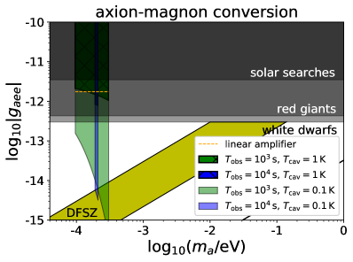
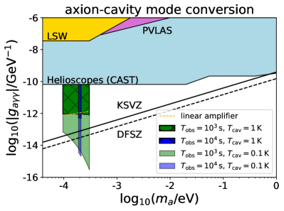
Figure 1: Sensitivity plot for $\text{SNR}=3$ under $T_{\text{total}}=10\,\text{years}$. Left: Sensitivity of the magnon detector on the axion-electron coupling $g_{aee}$ as a function of the axion mass $m_{a}$. The green and blue regions show the sensitivity for an ideal setup. The colors and styles of regions represent different setups; the observation time for each scan is set to be $T_{\mathrm{obs}}=10^{3}\,\mathrm{s}$ (green) or $10^{4}\,\mathrm{s}$ (blue), and the cavity temperature is $T_{\mathrm{cav}}=1\,\mathrm{K}$ (dark-meshed) or $0.1\,\mathrm{K}$ (light). The orange dashed line shows the sensitivity for a realistic setup with $T_{\mathrm{obs}}=10^{3}\,\mathrm{s}$ and $T_{\mathrm{cav}}\ll m_{a}$. Throughout the figure, the setup of $M_{\text{target}}=1\,\mathrm{kg}$, $\tau=2\,\mathrm{\mu s}$, $v_{a}=10^{-3}$, and $\sin^{2}\theta=0.5$ is assumed. Besides, the gray regions show the parameter region already excluded by other searches and the yellow region and the black solid line correspond to the prediction of the DFSZ model with $0.28\lesssim\tan\beta\lesssim 140$ and that of the KSVZ model, respectively. Right: Sensitivity of the cavity detector on the axion-photon coupling $g_{a\gamma\gamma}$ as a function of $m_{a}$. Similar to the left panel, the green and blue regions and orange lines show the sensitivities with $B_{0}=1\,\mathrm{T}$, $V_{\text{cav}}\mathcal{G}_{\text{cav}}=100\,\mathrm{cm}^{3}$, and $\tau_{\text{cav}}=2\,\mathrm{\mu s}$. The other shaded regions show the region excluded by other searches and the black dashed (solid) line corresponds to the prediction of the DFSZ (KSVZ) model.

In Fig. 1, we show the sensitivity of the magnon detector (left) and the cavity detector (right) with the total observation of $T_{\text{total}}=10\,\text{years}$. For an ideal setup, we use two different choices of the observation time $T_{\text{obs}}=10^{3}\,\mathrm{s}$ and $10^{4}\,\mathrm{s}$, which are shown by green and blue colors, respectively. We also use two different choices of the cavity temperature $T_{\mathrm{cav}}=1\,\mathrm{K}$ and $0.1\,\mathrm{K}$, which are shown by the dark-meshed and the light regions, respectively. For a realistic setup, we use the choice of $T_{\mathrm{obs}}=10^{3}\,\mathrm{s}$ and $T_{\mathrm{cav}}\ll m_{a}$ and the result is shown with an orange dashed line. The center of the scanned region of the axion mass is fixed to be $m_{a}=200\,\mathrm{\mu eV}$ and the width of the region is given by $\Delta m_{a}$ for each choice of $T_{\text{obs}}$.

In the left panel, the sensitivity on the dimensionless axion-electron coupling $g_{aee}\equiv m_{e}/f$ is shown as a function of the axion mass $m_{a}$, assuming the setup of $M_{\text{target}}=1\,\mathrm{kg}$, $\tau=2\,\mathrm{\mu s}$, $v_{a}=10^{-3}$, and $\sin^{2}\theta=0.5$. Gray regions correspond to the parameter space excluded by other searches using the bremsstrahlung from white dwarfs [70], the brightness of the tip of the red-giant branch in globular clusters [71], and the direct detection of solar axions at the EDELWEISS-II [72], the XENON100 [73], and the LUX [74] collaborations. Besides, the yellow region and the black solid line show the prediction for the DFSZ and KSVZ models, respectively. To obtain the DFSZ prediction, we variate $\tan\beta$, which is the ratio between vacuum expectation values of the two Higgs doublets, within $0.28\lesssim\tan\beta\lesssim 140$ as required by the perturbative unitarity of Yukawa couplings [75]. By comparing with the right panel, we can see that the axion search using the cavity mode has a better sensitivity than that using magnon excitation for the DFSZ and KSVZ models. At the same time, however, the sensitivity of the magnon detector reaches the DFSZ prediction for a relatively heavy mass due to the Boltzmann suppression of the noise rate according to Eq. (46). Thus, the figure shows the potential to probe the axion-electron coupling depending on the details of the model. It opens up a possibility to distinguish the KSVZ and DFSZ model by looking at the magnon-induced signal, once the DM signal is discovered at the cavity experiment.

In the right panel, the sensitivity on the axion-photon coupling $g_{a\gamma\gamma}\equiv C_{a\gamma}\alpha_{e}/(2\pi f)$ is shown, assuming the setup of $B_{0}=1\,\mathrm{T}$, $V_{\text{cav}}\mathcal{G}_{\text{cav}}=100\,\mathrm{cm}^{3}$, and $\tau_{\text{cav}}=2\,\mathrm{\mu s}$ in this case. Three shaded regions in $|g_{a\gamma\gamma}|\gtrsim 10^{-10}\,\mathrm{GeV}^{-1}$ correspond to the regions excluded by existing searches; the helioscope CAST [76], the Light-Shining-through-Walls (LSW) experiments such as the OSQAR [77], and the measurement of the vacuum magnetic birefringence at the PVLAS [78]. The black dashed (solid) line corresponds to the prediction of the DFSZ (KSVZ) model. We can see that the predicted values of $g_{a\gamma\gamma}$ around $m_{a}\simeq 200\,\mathrm{\mu eV}$ are covered by the cavity detector with the given setup.

4 Hidden photon conversion into magnon

4.1 Formulation

Let us consider a model with a massive hidden photon which has a kinetic mixing with hypercharge photon. In such a model, the hidden photon interacts with SM fields via

$$\mathcal{L}=-\frac{1}{4}H_{\mu\nu}H^{\mu\nu}-\frac{1}{4}B_{\mu\nu}B^{\mu\nu}+\frac{\epsilon_{Y}}{2}H_{\mu\nu}B^{\mu\nu}+\frac{1}{2}m_{H}^{2}H_{\mu}H^{\mu},$$ (49)

where $H_{\mu\nu}=\partial_{\mu}H_{\nu}-\partial_{\nu}H_{\mu}$ with $H_{\mu}$ being the hidden photon, $B_{\mu\nu}=\partial_{\mu}B_{\nu}-\partial_{\nu}B_{\mu}$ with $B_{\mu}$ being the hypercharge photon and $\Phi$ denotes the SM Higgs doublet. The kinetic terms of gauge bosons are diagonalized by the following transformation:

$$B_{\mu}^{\prime}=B_{\mu}-\epsilon_{Y}H_{\mu},~{}~{}~{}~{}~{}~{}H_{\mu}^{\prime}=\sqrt{1-\epsilon_{Y}^{2}}H_{\mu},$$ (50)

so that the kinetic term of the hidden photon and hypercharge photon and the hidden photon mass term become

$$\mathcal{L}=-\frac{1}{4}H^{\prime}_{\mu\nu}H^{\prime\mu\nu}-\frac{1}{4}B^{\prime}_{\mu\nu}B^{\prime\mu\nu}+\frac{1}{2}m_{H}^{\prime 2}H^{\prime}_{\mu}H^{\prime\mu},$$ (51)

where $m_{H}^{\prime 2}=m_{H}^{2}/(1-\epsilon_{Y}^{2})$. After the Higgs obtains a VEV, these gauge bosons, as well as the neutral weak gauge boson $(W^{3}_{\mu})$, are mixed. Denoting the Higgs VEV as $v\simeq 174\,$GeV, the gauge boson mass term is given by

$$\mathcal{L}_{\rm mass}=\frac{m_{Z}^{2}}{2}\left(c_{W}W_{\mu}^{3}-s_{W}B_{\mu}\right)^{2}+\frac{m_{H}^{\prime 2}}{2}H_{\mu}^{\prime 2}.$$ (52)

Here, $m_{Z}^{2}=(g_{W}^{2}+g_{Y}^{2})v^{2}/2$, $c_{W}=g_{W}/\sqrt{g_{W}^{2}+g_{Y}^{2}}$, where $s_{W}=g_{Y}/\sqrt{g_{W}^{2}+g_{Y}^{2}}$, $g_{W}$ is the weak gauge coupling and $g_{Y}$ is the hypercharge gauge coupling $(g_{Y}=e/c_{W})$. Besides, the SM fermions (denoted as $\psi$) are neutral for the hidden photon gauge interaction and hence the interactions between the SM fermions and hidden photon originate from

$$\mathcal{L}_{\rm int}=\overline{\psi}(Q_{Y}g_{Y}\gamma^{\mu}B_{\mu}+Q_{T_{3}}g_{W}\gamma^{\mu}W^{3}_{\mu})\psi,$$ (53)

where $Q_{Y}$ is the hypercharge of $\psi$ and $Q_{T_{3}}$ is the charge under $T_{3}$ rotation of SU(2).

The mass matrix in the $(W_{\mu}^{3},B_{\mu}^{\prime},H_{\mu}^{\prime})$ basis is

$$\mathcal{M}^{2}=m_{Z}^{2}\begin{pmatrix}c_{W}^{2}&-s_{W}c_{W}&s_{W}c_{W}\epsilon_{Y}/\sqrt{1-\epsilon_{Y}^{2}}\\ -s_{W}c_{W}&s_{W}^{2}&-s_{W}^{2}\epsilon_{Y}/\sqrt{1-\epsilon_{Y}^{2}}\\ s_{W}c_{W}\epsilon_{Y}/\sqrt{1-\epsilon_{Y}^{2}}&-s_{W}^{2}\epsilon_{Y}/\sqrt{1-\epsilon_{Y}^{2}}&s_{W}^{2}\epsilon_{Y}^{2}/(1-\epsilon_{Y}^{2})+m_{H}^{\prime 2}/m_{Z}^{2}\end{pmatrix}.$$ (54)

Up to the first order in $\epsilon_{Y}$, It is diagonalized by the following unitary transformation to go to the mass eigenstate $(Z_{\mu},A_{\mu},H_{\mu}^{\prime})$:

$$\begin{pmatrix}W_{\mu}^{3}\\ B_{\mu}^{\prime}\\ H_{\mu}^{\prime}\end{pmatrix}\simeq\begin{pmatrix}c_{W}&s_{W}&-s_{W}c_{W}\epsilon_{Y}\\ -s_{W}&c_{W}&s_{W}^{2}\epsilon_{Y}\\ s_{W}\epsilon_{Y}&0&1\end{pmatrix}\begin{pmatrix}Z_{\mu}\\ A_{\mu}\\ H_{\mu}^{\prime\prime}\end{pmatrix},$$ (55)

with the mass eigenvalues of $(m_{Z}^{2},0,m_{H}^{\prime 2})$.

After integrating out $Z$-boson, whose mass is much larger than the energy scale of our interest, the relevant part of the fermion interaction can be written as

$$\mathcal{L}_{\rm int}\supset-\epsilon\,eQ\,H_{\mu}^{\prime\prime}\,\overline{\psi}\gamma^{\mu}\psi,$$ (56)

where $Q=Q_{Y}+Q_{T_{3}}$ is the electromagnetic charge and $\epsilon\equiv\epsilon_{Y}c_{W}$. Thus, the hidden photon effectively couples to electromagnetic current with an effective coupling constant $\epsilon e$. The interaction Hamiltonian with electron in the non-relativistic limit is then given by

$$H_{\rm int}=-\frac{\epsilon eQ}{m_{e}}\sum_{\ell}\vec{B}_{H}(\vec{x}_{\ell})\cdot\vec{S}_{\ell},$$ (57)

where $\vec{B}_{H}\equiv\vec{\nabla}\times\vec{H}$ is the hidden magnetic field (see Appendix A).

We parametrize the hidden photon background as

$$H_{0}(t,\vec{x})= \,-\vec{v}_{H}\cdot\vec{\widetilde{H}}\cos\left(m_{H}t-m_{H}\vec{v}_{H}\cdot\vec{x}+\delta\right),$$ (58)

$$\vec{H}(t,\vec{x})= \,\vec{\widetilde{H}}\cos\left(m_{H}t-m_{H}\vec{v}_{H}\cdot\vec{x}+\delta\right),$$ (59)

to satisfy the equation of motion $(\square+m_{H}^{2})\vec{H}=0$ and the Lorentz condition $\partial_{\mu}H^{\mu}=0$. At the location of the ferromagnetic material, the hidden electric and magnetic fields are given by

$$\vec{E}_{H}\simeq \,\vec{\widetilde{H}}\,m_{H}\sin\left(m_{H}t+\delta\right),$$ (60)

$$\vec{B}_{H}\simeq \,\vec{v}_{H}\times\vec{\widetilde{H}}\,m_{H}\sin\left(m_{H}t+\delta\right).$$ (61)

The DM density is given by $\rho_{\rm DM}=m_{H}^{2}\widetilde{H}^{2}/2$.

The hidden photon-magnon interaction Hamiltonian is written as

$$H_{\rm int}=\frac{\epsilon em_{H}\widetilde{H}v_{H}}{m_{e}}\sum_{\ell}\vec{e}_{B}\cdot\vec{S}_{\ell}\sin\varphi\,\sin(m_{H}t+\delta),$$ (62)

where $\varphi$ denotes the angle between $\vec{v}_{H}$ and $\vec{H}$, and $\vec{e}_{B}$ is the unit vector of the direction of $\vec{B}_{H}$. It causes hidden photon-magnon conversion under the static magnetic field as in the case of the axion. Comparing (62) with the axion-magnon Hamiltonian (26), we can repeat the same analysis by just reinterpreting $1/f\to\epsilon e\sin\varphi/m_{e}$. Thus, referring to (39), the power obtained by this process is given by

$$\frac{dE_{\rm signal}}{dt}=\frac{(\epsilon e)^{2}\omega_{L}sN\rho_{\rm DM}v_{H}^{2}t}{8m_{e}^{2}}\sin^{2}\theta\sin^{2}\varphi,$$ (63)

where $\theta$ denotes the angle between $\vec{B}_{H}$ and $z$-axis. Note again that $t$ is limited by the hidden photon coherence time or magnon relaxation time (due to spin-lattice or spin-spin interactions), which we denote by $\tau$. The event rate is then

$$\left[\frac{dN_{\rm signal}}{dt}\right]_{\rm spin} =\frac{(\epsilon e)^{2}sN\rho_{\rm DM}v_{H}^{2}\tau}{8m_{e}^{2}}\sin^{2}\theta\sin^{2}\varphi$$

$$\simeq 9.6\times 10^{-5}\,{\rm s^{-1}}\left(\frac{\epsilon}{10^{-14}}\right)^{2}\left(\frac{M_{\text{target}}}{1\,\text{kg}}\right)\left(\frac{v_{H}}{10^{-3}}\right)^{2}\left(\frac{\tau}{2\,{\rm\mu s}}\right)\sin^{2}\theta\sin^{2}\varphi,$$ (64)

where we use the same setup like that in the previous section to convert $sN$ into $M_{\text{target}}$.

4.2 Sensitivity

So far we have discussed the hidden photon interaction with electron spin and its consequences for magnon excitation. However, as in the case of axion DM, the cavity setup itself also works as a hidden photon detector even without magnetic material [41, 2]. The background DM hidden photon generates the cavity mode through the kinetic mixing term and the photon event rate is estimated as [2]

$$\left[\frac{dN_{\rm signal}}{dt}\right]_{\rm mix} =\epsilon^{2}m_{H}\rho_{\rm DM}V_{\rm cav}\mathcal{G}_{\rm cav}{\rm min}\left[\tau_{H},\tau_{\rm cav}\right]$$ (65)

$$\simeq 1.4\times 10^{3}\,{\rm s^{-1}}\left(\frac{\epsilon}{10^{-14}}\right)^{2}\left(\frac{m_{H}}{10^{-4}\,{\rm eV}}\right)\left(\frac{V_{\rm cav}\mathcal{G}_{\rm cav}}{100\,{\rm cm^{3}}}\right)\left(\frac{\tau_{\rm cav}}{2\,{\rm\mu s}}\right),$$ (66)

where $\mathcal{G}_{\rm cav}$ is an $\mathcal{O}(1)$ form factor which may take a different value from the axion DM case. Comparing it with $\left[dN_{\rm signal}/dt\right]_{\rm spin}$, the signal induced by the mixing is expected to be much larger than the spin-induced ones. Note, however, that if each magnon event could be detected in other ways, i.e, without the use of cavity, the hidden photon interactions with spin and SM photon may be separately confirmed, which works as strong evidence of hidden photon DM. Conversely, if the DM signal is discovered in a cavity without magnetic material and the sizable spin-induced signal is also present, one can rule out the hidden photon DM.

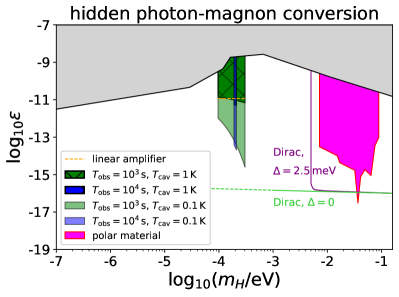
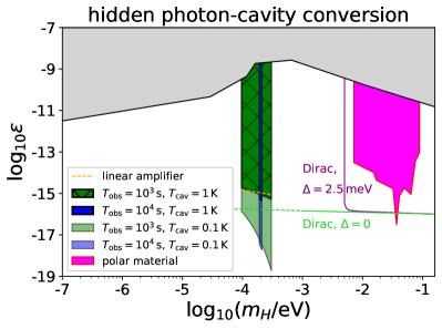
Figure 2: Sensitivity of the magnon (left) and cavity (right) detectors in the $m_{H}$ vs. $\epsilon$ plane. We use $M_{\text{target}}=1\,\text{kg}$ and $T_{\text{total}}=10\,\text{years}$. The other parameters are chosen as $v_{H}=10^{-3}$, $\tau=2\,\mathrm{\mu s}$, and $\sin^{2}\theta=\sin^{2}\varphi=1/2$. The green and blue colors correspond to an ideal setup case with $(\mathrm{SNR})=3$ and $T_{\text{obs}}=10^{3}\,\mathrm{s}$ and $10^{4}\,\text{s}$, respectively, and the dark-meshed and the light regions show those with $T_{\mathrm{cav}}=1\,\mathrm{K}$ and $0.1\,\mathrm{K}$, respectively. The orange dashed lines correspond to a realistic setup with $T_{\mathrm{obs}}=10^{3}\,\mathrm{s}$ and $T_{\mathrm{cav}}\ll m_{a}$. The gray region corresponds to the parameter space already excluded by other experiments. Magenta region shows the expected sensitivity of polar materials, while purple and light green lines show that of Dirac materials.

Let us estimate the experimental sensitivity as done in Sec. 3.2. In Fig. 2, we show the sensitivity of the magnon (left) and the cavity (right) detectors on the hidden photon with $M_{\text{target}}=1\,\text{kg}$ and $T_{\text{total}}=10\,\text{years}$. The center of the scan is fixed to be $m_{H}=200\,\mathrm{\mu eV}$. To derive the sensitivity, we use the parameter choices $v_{H}=10^{-3}$, $\tau=2\,\mathrm{\mu s}$, and $\sin^{2}\theta=\sin^{2}\varphi=1/2$. For an ideal setup, we again use two different choices of the observation time $T_{\text{obs}}=10^{3}\,\mathrm{s}$ (green) and $10^{4}\,\mathrm{s}$ (blue), while the dark-meshed and light regions show the sensitivities with $T_{\mathrm{cav}}=1\,\mathrm{K}$ and $T_{\mathrm{cav}}=0.1\,\mathrm{K}$, respectively. The orange dashed lines show the sensitivities of a realistic setup with $T_{\mathrm{obs}}=10^{3}\,\mathrm{s}$ and $T_{\mathrm{cav}}\ll m_{a}$. Also shown in gray color is the parameter region already excluded [79]; this includes constraints from spectral distortions [2], modifications to $N_{\text{eff}}$ [2], and stellar cooling [80, 81, 82]. The magenta region shows the expected sensitivity using polar materials with phonon excitation by the hidden photon absorption [47]. The purple (light green) solid line shows the expected sensitivity using Dirac materials with a band gap of $\Delta=2.5\,\mathrm{meV}$ ($\Delta=0$) [48], while the light green dotted line is an extrapolation of the sensitivity assuming that the electron excitation with energy of $\mathcal{O}(10^{-4})\,\mathrm{eV}$ can be detected. From the figure, we can see the strong potential of this setup on the hidden photon search. Even if we use a much shorter value of $T_{\text{obs}}$ than the canonical value adopted in the QUAX proposal, a much stronger bound on the kinetic mixing $\epsilon$ is obtained than the existing ones. For models with kinetic mixing between the photon and hidden photon DM, we can see that the cavity mode can cover a larger parameter region. It is notable that the magnon mode can also reach a parameter region which has not been explored yet. If one can separate the cavity signal and magnon-induced signal, it is in principle possible that the hidden photon DM scenario is confirmed by looking at the ratio of both the signals, although it might be challenging due to the weakness of the magnon signal.

Although we have fixed the central value of $m_{H}$ for the scan to be $200\,\mathrm{\mu eV}$, the choice of this value is not mandatory. The mass range to which this search method can be applied is estimated as follows. As for the heavier region, the strength of the magnetic field will put an upper bound on the applicability. The hidden photon mass of $200\,\mathrm{\mu eV}$ already corresponds to the magnetic field of $1.7\,\text{T}$, which should be amplified linearly as considering heavier mass. Thus a few times $10^{-4}\,\mathrm{eV}$ is considered to be the largest mass that can practically be probed. On the other hand, for the lighter region, the energy deposited to the detector from the hidden photon becomes comparable to the thermal noise when $m_{H}\sim 10^{-5}\,\mathrm{eV}$. This lower bound, however, may be loosened by further cooling the detector, though larger cavity may be needed to detect magnon-polariton as a final state particle.

So far, we have seen that the cavity mode has a better sensitivity than the magnon mode if the coupling to the hidden photon is dominated by the kinetic mixing given in Eq. (49). This conclusion is, however, model dependent. For example, one can consider a model where the electron has only the magnetic interaction with the hidden photon:

$$\mathcal{L}=-\frac{1}{4}H_{\mu\nu}H^{\mu\nu}-\frac{1}{4}B_{\mu\nu}B^{\mu\nu}+\frac{1}{2}m_{H}^{2}H_{\mu}H^{\mu}+\frac{m_{e}}{M^{2}}\overline{\psi}\sigma_{\mu\nu}\psi H^{\mu\nu},$$ (67)

with some cutoff scale $M$. In this case, the magnon-induced photon is practically the only possible signal and the strongest constraint on $\epsilon$, which is now reinterpreted as the effective interaction strength $m_{e}/M^{2}$, may be obtained from the magnon excitation.

5 Conclusions and discussion

We have shown that the light boson DM (axion and hidden photon) can be converted into magnon and it can be used as a DM detection method. Such an idea was already given in the QUAX proposal [29] for the axion DM detection and we have shown that a similar process happens for the hidden photon DM. A key observation is that the hidden photon has a magnetic interaction with electrons, which induces a spin wave or the magnon in the ferromagnetic/ferrimagnetic insulator. Since the magnon dispersion relation can be adjusted by applying the external magnetic field, one can scan the hidden photon DM mass. Unfortunately, such a spin-induced signal is smaller than the conventional hidden photon to SM conversion in the cavity, but it can be used to distinguish the axion DM (DFSZ or flaxion model) and hidden photon DM since the former predicts relatively large signal from the DM-magnon interaction.

Below we comment on ideas of hidden photon DM detection in the condensed-matter system. Refs. [44, 45] considered superconductor and semiconductor as a target material. The hidden photon is absorbed by electrons in the conducting band and it emits the (acoustic) phonon, hence it is a scattering process $\vec{H}+e\to P+e$, where $P$ denotes the phonon. Refs. [47, 49] also considered the hidden photon absorption by polar material, which has gapped optical phonon modes. It may be regarded as a hidden photon conversion process into an optical phonon, followed by the dissipation of the optical phonon. On the other hand, we focused on the hidden photon conversion into magnon in a ferromagnetic or ferrimagnetic insulator.

We have only considered resonant conversion into the magnon. It is rather regarded as a magnon-polariton so that the magnon effectively induces a cavity photon mode [29]. While the conversion rate is enhanced, one drawback of this idea is that it takes a long time to scan the wide range of DM mass. It is in principle possible that the magnon decays into several quanta, such as two magnons [83, 84] or magnon plus phonon [85]. Multi-phonon processes in the context of light DM detection was discussed in Refs. [86, 87, 88] for superfluid helium target and in Ref. [89] for crystal target. In such a case the kinematical constraint is weakened and wide mass range may be covered while the excitation rate is suppressed. We keep a detailed study of this issue as a future work [90].

Here we point out that other ideas for axion DM detection may also be used as a hidden photon detector. In Ref. [22] a novel method to detect axion DM was proposed using the topological antiferromagnet insulator. The axion is assumed to have an interaction with photon through the Chern-Simons term like (43). In a topological magnetic insulator, the magnon may also have a similar Chern-Simons coupling to the photon [91]. Under the applied magnetic field, the background DM axion is converted into the electric field. It is again converted into the magnon under the magnetic field, which induces photon emission due to the boundary effect. By choosing the magnetic field appropriately, the intermediate magnon hits the resonance to enhance the signal. Notably, the same idea also applies to the hidden photon DM. The hidden photon DM is converted to the electric field through the kinetic mixing

$$\mathcal{L}=\frac{\epsilon}{2}H_{\mu\nu}F^{\mu\nu}=-\epsilon(\vec{E}_{H}\cdot\vec{E}-\vec{B}_{H}\cdot\vec{B}).$$ (68)

Given $|\vec{E}_{H}|\gg|\vec{B}_{H}|$, the hidden photon DM mainly produces electric fields. Then it is converted into the magnon under the magnetic field, as explained above. Comparing (43) with (68), one obtains a sensitivity on the kinetic mixing parameter $\epsilon$ by replacing the sensitivity on $(m_{a},f)$ obtained in Ref. [22] through the correspondence

$$\epsilon=C_{a\gamma}\frac{\alpha_{e}}{2\pi}\frac{B_{0}}{m_{a}f}\simeq 2\times 10^{-17}\,C_{a\gamma}\left(\frac{10^{10}\,{\rm GeV}}{f}\right)\left(\frac{1\,{\rm meV}}{m_{a}}\right)\left(\frac{B_{0}}{1\,{\rm T}}\right),$$ (69)

where $B_{0}$ is the applied magnetic field. Thus it may have a very good sensitivity on the hidden photon DM. We will also come back to this issue in a separate publication.

Appendix A Effective Hamiltonian of magnon

Here, we derive the magnon couplings to axion and hidden photon, starting from the Lorentz-invariant quantum field theory (QFT). Let us denote the electron field operator in the QFT as

$$\psi(x)=\int\frac{d^{3}p}{(2\pi)^{3}\sqrt{2p_{0}}}\sum_{s}a_{\vec{p},s}u_{\vec{p},s}e^{-ipx},$$ (70)

where $p_{0}\equiv\sqrt{\vec{p}^{2}+m_{e}^{2}}$ and

$$u_{\vec{p},s}=\left(\begin{array}[]{c}\sqrt{p_{0}+m}\,\chi_{s}\\ \sqrt{p_{0}-m}\,\vec{e}_{p}\cdot\vec{\sigma}\chi_{s}\end{array}\right),$$ (73)

with $\vec{e}_{p}$ denoting the unit vector pointing to the direction of $\vec{p}$, and $\chi_{s}=(1,0)^{T}$ or $(0,1)^{T}$. (We adopt the Dirac representation of the $\gamma$-matrices.) Besides, the creation and annihilation operators of the electron are denoted as $a_{\vec{p},s}$ and $a^{\dagger}_{\vec{p},s}$, respectively, which satisfy $\{a_{\vec{p},s},a^{\dagger}_{\vec{p}^{\prime},s^{\prime}}\}=(2\pi)^{3}\delta(\vec{p}-\vec{p}^{\prime})\delta_{ss^{\prime}}$. We are interested in the system containing only the electron, so we neglect the positron degrees freedom. Concentrating on non-relativistic degrees of freedom, the spin operator in the QFT is given by

$$\vec{S}^{\rm(QFT)}=\int\frac{d^{3}p}{(2\pi)^{3}}\sum_{s,s^{\prime}}a^{\dagger}_{\vec{p},s}a_{\vec{p},s^{\prime}}\chi_{s}^{\dagger}\vec{\sigma}\chi_{s^{\prime}}.$$ (74)

Notice that the spin operator given above satisfies the relevant commutation relations.

We expect that the total spin operator in the QFT is matched to that in the Heisenberg model as

$$\vec{S}^{\rm(QFT)}\rightarrow\sum_{\ell}\vec{S}_{\ell}.$$ (75)

Hereafter, we derive the effective interaction of the magnon using this matching condition as well as assuming the locality of the interaction.

In the model with the hidden photon, the magnon couples to the hidden photon via the kinetic mixing with the hypercharge photon given in Eq. (49). Because we are interested in the energy scale much lower than the electron mass, we can concentrate on the effective field theory that contains only non-relativistic electron, photon, and hidden photon. In such a case, the only relevant interaction of the hidden photon with the electron is from the mixing of the hidden photon with the ordinary photon, and is given by

$${\cal L}=-\epsilon eQH_{\mu}\bar{\psi}\gamma^{\mu}\psi,$$ (76)

where $Q$ is the charge of the electron (in units of $e$), and $\epsilon\equiv\epsilon_{Y}c_{W}$. Then, we can find

$$H_{\rm int}\simeq\frac{\epsilon eQ}{2m_{e}}\epsilon_{ijk}\int d^{3}x\frac{d^{3}p}{(2\pi)^{3}}\frac{d^{3}p^{\prime}}{(2\pi)^{3}}\sum_{s,s^{\prime}}a^{\dagger}_{\vec{p},s}a_{\vec{p}^{\prime},s^{\prime}}(\partial_{i}H_{j})e^{i(p-p^{\prime})x}\chi^{\dagger}_{s}\sigma^{k}\chi_{s^{\prime}}+\epsilon\int d^{3}xH_{\mu}j^{\mu},$$ (77)

where

$$j^{0}\equiv \,-eQ\int\frac{d^{3}p}{(2\pi)^{3}}\frac{d^{3}p^{\prime}}{(2\pi)^{3}}\sum_{s}a^{\dagger}_{\vec{p},s}a_{\vec{p}^{\prime},s}e^{i(p-p^{\prime})x},$$ (78)

$$\vec{j}\equiv \,-eQ\int\frac{d^{3}p}{(2\pi)^{3}}\frac{d^{3}p^{\prime}}{(2\pi)^{3}}\sum_{s}\frac{\vec{p}+\vec{p^{\prime}}}{2m_{e}}a^{\dagger}_{\vec{p},s}a_{\vec{p}^{\prime},s}e^{i(p-p^{\prime})x}.$$ (79)

The first term of the right-hand side gives the coupling of magnon to the hidden photon. Assuming the locality of the interaction, and using the (discrete) translational invariance of the system, we expect that the effective interaction between the spin (i.e., magnon) and the hidden photon contains the following term:

$$H_{\rm int}\ni-\frac{\epsilon eQ}{m_{e}}\sum_{\ell}\vec{B}_{H}(\vec{x}_{\ell})\cdot\vec{S}_{\ell},$$ (80)

with $\vec{B}_{H}$ being the hidden magnetic field. The second term of the right-hand side of Eq. (77) is the coupling of the (ordinary) current with the vector potential of the hidden photon. So far, we have concentrated on the coupling between the hidden photon and the electron. The hidden photon coupling to the nucleon can be also derived similarly. The nucleon counterpart of the second term of Eq. (77) may cause the hidden photon-phonon conversion. However, it is not kinematically allowed unless the (optical) phonon energy gap happens to be close to the hidden photon mass. The hidden photon absorption by polar material was considered in Refs. [47, 49] for the mass range of $10^{-2}$–$10^{-1}$ eV. We consider lighter DM mass region around meV, so we neglect such an effect.

The magnon-axion coupling originates from the axion-electron interaction (see the last term of Eq. (23)). Using the fact that, in the non-relativistic limit,

$$\vec{S}^{\rm(QFT)}\simeq\frac{1}{2}\int d^{3}x\bar{\psi}\vec{\gamma}\gamma_{5}\psi,$$ (81)

we obtain the coupling of an axion to a magnon as

$$H_{\rm int}=\frac{1}{f}\sum_{\ell}\vec{\nabla}a(x_{\ell})\cdot\vec{S}_{\ell}.$$ (82)

Appendix B Classical calculation of conversion rate

Let us reproduce the same result with classical calculation [29]. We treat the magnetization $\vec{M}$ of the material as a classical magnetic moment and study its motion under the classical axion background. Neglecting damping effects due to radiation, spin-spin or spin-lattice interactions, the classical equation of motion is given by

$$\dot{\vec{M}}=\frac{e}{m_{e}}\vec{M}\times\vec{B},~{}~{}~{}~{}~{}~{}\vec{B}=B_{z}^{0}\vec{e}_{z}+\vec{B}_{a}.$$ (83)

We find

$$\ddot{M}_{x}+\omega_{L}^{2}M_{x}=\frac{eM_{z}}{m_{e}}\left(\omega_{L}B_{x}^{a}-\dot{B}_{a}^{y}\right),$$ (84)

$$\ddot{M}_{y}+\omega_{L}^{2}M_{y}=\frac{eM_{z}}{m_{e}}\left(\omega_{L}B_{y}^{a}+\dot{B}_{a}^{x}\right).$$ (85)

We can rewrite these equations by using $M_{\pm}\equiv M_{x}\pm iM_{y}$ as

$$\ddot{M}_{+}+\omega_{L}^{2}M_{+}=i\frac{esNm_{a}^{2}a_{0}v^{+}}{m_{e}}e^{-i(m_{a}t+\delta)},$$ (86)

$$\ddot{M}_{-}+\omega_{L}^{2}M_{-}=-i\frac{esNm_{a}^{2}a_{0}v^{-}}{m_{e}}e^{i(m_{a}t+\delta)}.$$ (87)

The solution is

$$M_{+}(t)=\frac{i\widetilde{V}e^{-i(m_{a}t+\delta)}}{m_{a}^{2}-\omega_{L}^{2}}\left[-1+e^{im_{a}t}\left(\cos(\omega_{L}t)-i\frac{m_{a}}{\omega_{L}}\sin(\omega_{L}t)\right)\right]+\frac{i\widetilde{V}\sin(\omega_{L}t)\sin\delta}{m_{a}\omega_{L}},$$ (88)

where

$$\widetilde{V}\equiv\frac{esNm_{a}^{2}a_{0}v_{a}^{+}}{m_{e}f}.$$ (89)

Taking the limit $\omega_{L}=m_{a}$, we obtain

$$M_{+}(t)\simeq\frac{i\widetilde{V}te^{-i(m_{a}t+\delta)}}{2m_{a}},~{}~{}~{}~{}~{}~{}M_{-}(t)\simeq-\frac{i\widetilde{V}^{*}te^{i(m_{a}t+\delta)}}{2m_{a}},$$ (90)

for $m_{a}t\gg 1$. The power obtained by the axion wind is then estimated as

$$\frac{dE_{M}}{dt}=\frac{d}{dt}(\vec{B}\cdot\vec{M})\simeq\frac{sN\rho_{\rm DM}m_{a}(v_{a}^{x2}+v_{a}^{y2})t}{f^{2}}\sin^{2}(m_{a}t+\delta).$$ (91)

After averaging $\sin^{2}(m_{a}t+\delta)=1/2$, it is consistent with (39).

References

- [1] J. Jaeckel and A. Ringwald, Ann. Rev. Nucl. Part. Sci. 60, 405 (2010) [arXiv:1002.0329 [hep-ph]].
- [2] P. Arias, D. Cadamuro, M. Goodsell, J. Jaeckel, J. Redondo and A. Ringwald, JCAP 1206, 013 (2012) [arXiv:1201.5902 [hep-ph]].
- [3] J. Preskill, M. B. Wise and F. Wilczek, Phys. Lett. B 120, 127 (1983).
- [4] L. F. Abbott and P. Sikivie, Phys. Lett. B 120, 133 (1983).
- [5] M. Dine and W. Fischler, Phys. Lett. B 120, 137 (1983).
- [6] J. E. Kim, Phys. Rept. 150, 1 (1987).
- [7] M. Kawasaki and K. Nakayama, Ann. Rev. Nucl. Part. Sci. 63, 69 (2013) [arXiv:1301.1123 [hep-ph]].
- [8] P. Svrcek and E. Witten, JHEP 0606, 051 (2006) [hep-th/0605206].
- [9] A. Arvanitaki, S. Dimopoulos, S. Dubovsky, N. Kaloper and J. March-Russell, Phys. Rev. D 81, 123530 (2010) [arXiv:0905.4720 [hep-th]].
- [10] M. Cicoli, M. Goodsell and A. Ringwald, JHEP 1210, 146 (2012) [arXiv:1206.0819 [hep-th]].
- [11] P. Sikivie, Phys. Rev. Lett. 51, 1415 (1983) Erratum: [Phys. Rev. Lett. 52, 695 (1984)].
- [12] R. Bradley, J. Clarke, D. Kinion, L. J. Rosenberg, K. van Bibber, S. Matsuki, M. Muck and P. Sikivie, Rev. Mod. Phys. 75, 777 (2003).
- [13] S. J. Asztalos et al. [ADMX Collaboration], Phys. Rev. Lett. 104, 041301 (2010) [arXiv:0910.5914 [astro-ph.CO]].
- [14] L. Zhong et al. [HAYSTAC Collaboration], Phys. Rev. D 97, no. 9, 092001 (2018) [arXiv:1803.03690 [hep-ex]].
- [15] B. T. McAllister, G. Flower, E. N. Ivanov, M. Goryachev, J. Bourhill and M. E. Tobar, Phys. Dark Univ. 18, 67 (2017) [arXiv:1706.00209 [physics.ins-det]].
- [16] D. Alesini, D. Babusci, D. Di Gioacchino, C. Gatti, G. Lamanna and C. Ligi, arXiv:1707.06010 [physics.ins-det].
- [17] Y. K. Semertzidis et al., arXiv:1910.11591 [physics.ins-det].
- [18] D. Horns, J. Jaeckel, A. Lindner, A. Lobanov, J. Redondo and A. Ringwald, JCAP 1304, 016 (2013) [arXiv:1212.2970 [hep-ph]].
- [19] J. Jaeckel and J. Redondo, Phys. Rev. D 88, no. 11, 115002 (2013) [arXiv:1308.1103 [hep-ph]].
- [20] A. Caldwell et al. [MADMAX Working Group], Phys. Rev. Lett. 118, no. 9, 091801 (2017) [arXiv:1611.05865 [physics.ins-det]].
- [21] Y. Kahn, B. R. Safdi and J. Thaler, Phys. Rev. Lett. 117, no. 14, 141801 (2016) [arXiv:1602.01086 [hep-ph]].
- [22] D. J. E. Marsh, K. C. Fong, E. W. Lentz, L. Smejkal and M. N. Ali, Phys. Rev. Lett. 123, no. 12, 121601 (2019) [arXiv:1807.08810 [hep-ph]].
- [23] I. Obata, T. Fujita and Y. Michimura, Phys. Rev. Lett. 121, no. 16, 161301 (2018) [arXiv:1805.11753 [astro-ph.CO]].
- [24] K. Nagano, T. Fujita, Y. Michimura and I. Obata, Phys. Rev. Lett. 123, no. 11, 111301 (2019) [arXiv:1903.02017 [hep-ph]].
- [25] M. Lawson, A. J. Millar, M. Pancaldi, E. Vitagliano and F. Wilczek, Phys. Rev. Lett. 123 (2019) no.14, 141802 [arXiv:1904.11872 [hep-ph]].
- [26] M. Zarei, S. Shakeri, M. Abdi, D. J. E. Marsh and S. Matarrese, arXiv:1910.09973 [hep-ph].
- [27] D. Budker, P. W. Graham, M. Ledbetter, S. Rajendran and A. Sushkov, Phys. Rev. X 4, no. 2, 021030 (2014) [arXiv:1306.6089 [hep-ph]].
- [28] R. Barbieri, M. Cerdonio, G. Fiorentini and S. Vitale, Phys. Lett. B 226, 357 (1989).
- [29] R. Barbieri et al., Phys. Dark Univ. 15, 135 (2017) [arXiv:1606.02201 [hep-ph]].
- [30] N. Crescini et al., arXiv:2001.08940 [hep-ex].
- [31] M. Cicoli, M. Goodsell, J. Jaeckel and A. Ringwald, JHEP 1107, 114 (2011) [arXiv:1103.3705 [hep-th]].
- [32] P. Agrawal, N. Kitajima, M. Reece, T. Sekiguchi and F. Takahashi, arXiv:1810.07188 [hep-ph].
- [33] R. T. Co, A. Pierce, Z. Zhang and Y. Zhao, Phys. Rev. D 99, no. 7, 075002 (2019) [arXiv:1810.07196 [hep-ph]].
- [34] M. Bastero-Gil, J. Santiago, L. Ubaldi and R. Vega-Morales, JCAP 1904, no. 04, 015 (2019) [arXiv:1810.07208 [hep-ph]].
- [35] J. A. Dror, K. Harigaya and V. Narayan, Phys. Rev. D 99, no. 3, 035036 (2019) [arXiv:1810.07195 [hep-ph]].
- [36] A. J. Long and L. T. Wang, Phys. Rev. D 99, no. 6, 063529 (2019) [arXiv:1901.03312 [hep-ph]].
- [37] P. W. Graham, J. Mardon and S. Rajendran, Phys. Rev. D 93, no. 10, 103520 (2016) [arXiv:1504.02102 [hep-ph]].
- [38] Y. Ema, K. Nakayama and Y. Tang, JHEP 1907, 060 (2019) [arXiv:1903.10973 [hep-ph]].
- [39] G. Alonso-Alvarez, T. Hugle and J. Jaeckel, arXiv:1905.09836 [hep-ph].
- [40] K. Nakayama, JCAP 1910, no. 10, 019 (2019) [arXiv:1907.06243 [hep-ph]].
- [41] A. Wagner et al. [ADMX Collaboration], Phys. Rev. Lett. 105, 171801 (2010) [arXiv:1007.3766 [hep-ex]].
- [42] S. R. Parker, J. G. Hartnett, R. G. Povey and M. E. Tobar, Phys. Rev. D 88, 112004 (2013) [arXiv:1410.5244 [hep-ex]].
- [43] S. Chaudhuri, P. W. Graham, K. Irwin, J. Mardon, S. Rajendran and Y. Zhao, Phys. Rev. D 92, no. 7, 075012 (2015) [arXiv:1411.7382 [hep-ph]].
- [44] Y. Hochberg, T. Lin and K. M. Zurek, Phys. Rev. D 94, no. 1, 015019 (2016) [arXiv:1604.06800 [hep-ph]].
- [45] Y. Hochberg, T. Lin and K. M. Zurek, Phys. Rev. D 95, no. 2, 023013 (2017) [arXiv:1608.01994 [hep-ph]].
- [46] I. M. Bloch, R. Essig, K. Tobioka, T. Volansky and T. T. Yu, JHEP 1706, 087 (2017) [arXiv:1608.02123 [hep-ph]].
- [47] S. Knapen, T. Lin, M. Pyle and K. M. Zurek, Phys. Lett. B 785, 386 (2018) [arXiv:1712.06598 [hep-ph]].
- [48] Y. Hochberg et al., Phys. Rev. D 97 (2018) no.1, 015004 [arXiv:1708.08929 [hep-ph]].
- [49] S. Griffin, S. Knapen, T. Lin and K. M. Zurek, Phys. Rev. D 98, no. 11, 115034 (2018) [arXiv:1807.10291 [hep-ph]].
- [50] A. Arvanitaki, S. Dimopoulos and K. Van Tilburg, Phys. Rev. X 8, no. 4, 041001 (2018) [arXiv:1709.05354 [hep-ph]].
- [51] M. Baryakhtar, J. Huang and R. Lasenby, Phys. Rev. D 98, no. 3, 035006 (2018) [arXiv:1803.11455 [hep-ph]].
- [52] C. Herring and C. Kittel, Phys. Rev. 81, 869 (1951).
- [53] A. G. Gurevich, G. A. Melkov, “Magnetization Oscillation and Waves”, CRC Press (1996).
- [54] V. Cherepanov, I. Kolokolov and V. L’vov, Physics Reports 229, 81 (1993).
- [55] H. Watanabe and H. Murayama, Phys. Rev. Lett. 108 (2012) 251602 [arXiv:1203.0609 [hep-th]].
- [56] Y. Hidaka, Phys. Rev. Lett. 110, no.9, 091601 (2013) [arXiv:1203.1494 [hep-th]].
- [57] T. Trickle, Z. Zhang and K. M. Zurek, arXiv:1905.13744 [hep-ph].
- [58] G. Flower, J. Bourhill, M. Goryachev and M. E. Tobar, Phys. Dark Univ. 25, 100306 (2019) [arXiv:1811.09348 [physics.ins-det]].
- [59] A. R. Zhitnitsky, Sov. J. Nucl. Phys. 31, 260 (1980) [Yad. Fiz. 31, 497 (1980)].
- [60] M. Dine, W. Fischler and M. Srednicki, Phys. Lett. 104B, 199 (1981).
- [61] Y. Ema, K. Hamaguchi, T. Moroi and K. Nakayama, JHEP 1701, 096 (2017) [arXiv:1612.05492 [hep-ph]].
- [62] L. Calibbi, F. Goertz, D. Redigolo, R. Ziegler and J. Zupan, Phys. Rev. D 95, no. 9, 095009 (2017) [arXiv:1612.08040 [hep-ph]].
- [63] X. Zhang, C. Zou, L. Jiang and H. X. Tang, Phys. Rev. Lett. 113, 156401 (2014).
- [64] Y. Tabuchi, S. Ishino, T. Ishikawa, R. Yamazaki, K. Usami and Y. Nakamura, Phys. Rev. Lett. 113, 083603 (2014) [arXiv:1405.1913].
- [65] Y. Tabuchi, S. Ishino, A. Noguchi, T. Ishikawa, R. Yamazaki and K. Usami, Comp. Rend. Phys. 17, 729 (2016) [arXiv:1508.05290].
- [66] J. E. Kim, Phys. Rev. Lett. 43, 103 (1979).
- [67] M. A. Shifman, A. I. Vainshtein and V. I. Zakharov, Nucl. Phys. B 166, 493 (1980).
- [68] S. Lamoreaux, K. van Bibber, K. Lehnert and G. Carosi, Phys. Rev. D 88 (2013) no.3, 035020 [arXiv:1306.3591 [physics.ins-det]].
- [69] L. Capparelli, G. Cavoto, J. Ferretti, F. Giazotto, A. Polosa and P. Spagnolo, Phys. Dark Univ. 12 (2016), 37-44 [arXiv:1510.06892 [hep-ph]].
- [70] M. M. Miller Bertolami, B. E. Melendez, L. G. Althaus and J. Isern, JCAP 1410 (2014) 069 [arXiv:1406.7712 [hep-ph]].
- [71] N. Viaux, M. Catelan, P. B. Stetson, G. Raffelt, J. Redondo, A. A. R. Valcarce and A. Weiss, Phys. Rev. Lett. 111 (2013) 231301 [arXiv:1311.1669 [astro-ph.SR]].
- [72] E. Armengaud et al., JCAP 1311 (2013) 067 [arXiv:1307.1488 [astro-ph.CO]].
- [73] E. Aprile et al. [XENON100 Collaboration], Phys. Rev. D 90 (2014) no.6, 062009 Erratum: [Phys. Rev. D 95 (2017) no.2, 029904] [arXiv:1404.1455 [astro-ph.CO]].
- [74] D. S. Akerib et al. [LUX Collaboration], Phys. Rev. Lett. 118 (2017) no.26, 261301 [arXiv:1704.02297 [astro-ph.CO]].
- [75] C. Y. Chen and S. Dawson, Phys. Rev. D 87 (2013) 055016 [arXiv:1301.0309 [hep-ph]].
- [76] V. Anastassopoulos et al. [CAST Collaboration], Nature Phys. 13 (2017) 584 [arXiv:1705.02290 [hep-ex]].
- [77] R. Ballou et al. [OSQAR Collaboration], Phys. Rev. D 92 (2015) no.9, 092002 [arXiv:1506.08082 [hep-ex]].
- [78] F. Della Valle, A. Ejlli, U. Gastaldi, G. Messineo, E. Milotti, R. Pengo, G. Ruoso and G. Zavattini, Eur. Phys. J. C 76 (2016) no.1, 24 [arXiv:1510.08052 [physics.optics]].
- [79] S. D. McDermott and S. J. Witte, arXiv:1911.05086 [hep-ph].
- [80] H. An, M. Pospelov and J. Pradler, Phys. Lett. B 725 (2013) 190 [arXiv:1302.3884 [hep-ph]].
- [81] J. Redondo and G. Raffelt, JCAP 1308 (2013) 034 [arXiv:1305.2920 [hep-ph]].
- [82] N. Vinyoles, A. Serenelli, F. L. Villante, S. Basu, J. Redondo and J. Isern, JCAP 1510 (2015) 015 [arXiv:1501.01639 [astro-ph.SR]].
- [83] A. Kreisel, F. Sauli, L. Bartosch and P. Kopietz, Eur. Phys. J. B 71, 59 (2009) [arXiv:0903.2847].
- [84] A. Ruckriegel, P. Kopietz, D. A. Bozhko, A. A. Serga and B. Hillebrands, Phys. Rev. B 89, 184413 (2014) [arXiv:1402.6575].
- [85] S. Streib, N. Vidal-Silva, K. Shen and G. E. W. Bauer, Phys. Rev. B 99, 184442 (2019) [arXiv:1906.01042].
- [86] K. Schutz and K. M. Zurek, Phys. Rev. Lett. 117, no. 12, 121302 (2016) [arXiv:1604.08206 [hep-ph]].
- [87] S. Knapen, T. Lin and K. M. Zurek, Phys. Rev. D 95, no. 5, 056019 (2017) [arXiv:1611.06228 [hep-ph]].
- [88] F. Acanfora, A. Esposito and A. D. Polosa, Eur. Phys. J. C 79, no. 7, 549 (2019) [arXiv:1902.02361 [hep-ph]].
- [89] B. Campbell-Deem, P. Cox, S. Knapen, T. Lin and T. Melia, arXiv:1911.03482 [hep-ph].
- [90] S. Chigusa, T. Moroi and K.Nakayama, in preparation.
- [91] R. Li, J. Wang, X. L. Qi, S. C. Zhang, Nature Phys. 6, 284 (2010) [arXiv:0908.1537].