Global simulations of stellar dynamos

Abstract

The dynamo mechanism, responsible for the solar magnetic activity, is still an open problem in astrophysics. Different theories proposed to explain such phenomena have failed in reproducing the observational properties of the solar magnetism. Thus, ab-initio computational modeling of the convective dynamo in a spherical shell turns out as the best alternative to tackle this problem. In this work we review the efforts performed in global simulations over the past decades. Regarding the development and sustain of mean-flows, as well as mean magnetic field, we discuss the points of agreement and divergence between the different modeling strategies. Special attention is given to the implicit large-eddy simulations performed with the EULAG-MHD code.

1 Introduction

The Sun exhibits a large-scale magnetic field which is believed to be driven by a dynamo somewhere in its interior. As a consequence of the dynamo several processes in the upper layers of the Sun define the solar activity (i.e., the 11-years sunspot cycle, the solar wind, coronal mass ejections and flares). It establishes a close interaction between the Sun and the earth defining the space weather and, perhaps, influencing long term variations of the earth’s temperature. Besides being fascinating as a physical problem, the astrophysical dynamo is a highly relevant area for our society.

The main properties of the solar cycle are presented in Fig. 1(top panel) and can be summarized as follow: (1) Sunspots appear in pairs of opposite polarity at latitudes of about $30^{\circ}$ and migrate towards the equator, (2) Spots in the northern hemisphere have the opposite polarity than their analogs in the southern hemisphere, (3) When the number of sunspots is maximum, the poloidal field reaches its minimum and reverses polarity, (4) accordingly, when the poloidal field is maximum, sunspots of a new cycle start to appear with opposite polarity in both hemispheres.

In addition to the solar data, recent observations of magnetic fields in main sequence stars of types F, G and K have imposed further constrains to the dynamo mechanism. Observations indicate two important relations between rotational period of the stars, $P_{\rm rot}$ and the observed magnetic field. First, the field strength exhibits two regimes: for fast rotation it is independent of $P_{\rm rot}$, for slow rotation the field amplitude decays with $P_{\rm rot}$ with power law dependence (e.g. Wright et al., 2011; Vidotto et al., 2014). The second relation regards the stars that exhibit activity cycles. A comparison between the magnetic cycle period, $P_{\rm cyc}$, and $P_{\rm rot}$ shows two regimes of activity, the so called active and inactive branches. For both of them, the longer $P_{\rm rot}$, the longer the $P_{\rm cyc}$ (Fig 1, bottom-right).

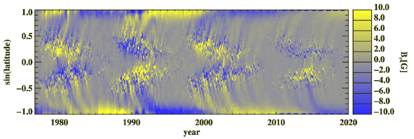
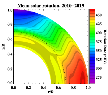
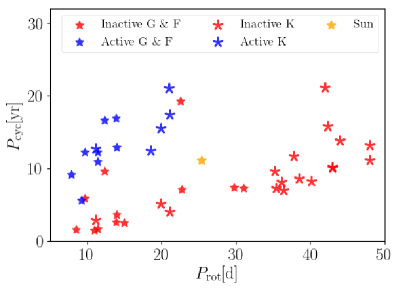
Figure 1: Top: time-latitude butterfly diagram (courtesy: A. Kosovichev); bottom-left: solar differential rotation (courtesy: A. Kosovichev); bottom-right: relation between $P_{\rm rot}$ and $P_{\rm cyc}$. The blue and red stars correspond to the observed active and inactive branches, respectively. The data was taken from Brandenburg et al. (2017).

Models to understand the solar/stellar dynamo problem are based on the theoretical framework known as mean-field dynamo theory (Parker, 1955; Steenbeck et al., 1966). It describes the generation of the mean magnetic field as the results of the inductive action of large-scale shear-flows ($\Omega$-effect) and small scale, turbulent, helical motions and currents ($\alpha$-effect). The properties of the $\Omega$-effect, i.e., the solar differential rotation, have been accurately identified by helioseismology (Fig. 1, bottom-left). Recent asteroseismology results have inferred that similar rotational shear profiles occur in solar type stars (Benomar et al., 2018). On the other side, the values and profiles of the $\alpha$-effect in the solar convection zone are uncertain. Some heuristic guesses for these contribution have found some success in reproducing the main characteristics of the solar cycle, nevertheless the results are ambiguous.

From the seminal work of Gilman & Miller (1981), three dimensional, first principles, global simulations were developed with the goal of unambiguously determine the location and properties of the dynamo sources. These models have been successful in reproducing and explaining the mechanisms that sustain the differential rotation (DR, see e.g., Miesch et al., 2006; Käpylä et al., 2011; Guerrero et al., 2013; Featherstone & Miesch, 2015), yet the magnetism has still some caveats. The growing of magnetic field in spherical turbulent convection resembling the solar case was obtained by Brun et al. (2004). They found magnetic fields with erratic behaviour without large-scale dynamics. More recently, Ghizaru et al. (2010) obtained for the first time cyclic dynamo action in a simulation using implicit sub-grid scale (SGS) modeling with the EULAG-MHD code. The magnetic cycle period of their simulation was about $60$ years, yet the migration of the magnetic field did not reproduce quite well the solar activity pattern. Later on, other groups have obtained oscillatory dynamos (e.g., Käpylä et al., 2012; Augustson et al., 2015) in spherical shells that consider only the convection zone. Their results are characterized by short dynamo cycle periods. Guerrero et al. (2016a) compared dynamo models with and without the radial shear layer at the interface between the radiative and the convective zone, the tachocline. They found important differences in the process of generating large scale magnetic fields and noticed that when the tachocline is included, $P_{\rm cyc}$ could be of the order of decades.

More recently the role of rotation was explored for simulations mimicking the solar interior. At odds with the observations, simulations including the convection zone only found that the cycle period decreases as the rotational period increases (Strugarek et al., 2017). On the other hand, Guerrero et al. (2019b) found proportionality between $P_{\rm cyc}$ and $P_{\rm rot}$ in simulations including also a fraction of the convection zone. The results, however, do not completely fit to the active or inactive branches of activity.

The numerical resolution used in the simulations discussed above is still far from capturing all the relevant scales of the solar (or stellar) interior. To the date, the simulations with highest resolution were run for less than $100$ years (Viviani et al., 2018; Hotta et al., 2016). The simulations of Hotta et al. (2016) have the maximal resolution reported in the literature and were run for $50$ yr. These simulations show reversals of magnetic field and, more importantly, are able to develop small scale dynamo action. Thus, the contribution of the small scale Maxwell stresses is captured in the simulations. Unfortunately, the characteristics of the magnetic field, evolution and periodicity, still diverge from the solar case. Parametric analyses at this resolution are still prohibitive. For simulations where the cycle periods are of the order of decades, the evolution time should be several hundred years for the variables to achieve statistically steady state. Therefore, large computing resources are needed.

The results described above make clear that in spite of the recent progress in observations and the development of high resolution simulations, the solar/stellar dynamo problem is not closed. There are some convergent results from which we have learn much about the behavior of stellar interiors. However, there is not yet a complete theory to satisfactory explain the details captured by the observations. In this work we review the recent advances in ab-initio global simulations of solar and stellar dynamos. We discuss the encouraging results as well as the caveats in the different approaches of global modeling. Even though great progress has been done in simulating fully convective stars, we focus here in solar-like stars with an inner radiative zone and a convective envelope.

This paper is organized as follows. In the following section we describe the equations of magnetohydrodynamics (MHD), the framework on which the global simulations are built, and some characteristics of the simulations setups. In §2.2 we discuss the direct numerical simulations and the large eddy simulations approaches for modeling rotating turbulent convection. In §3 and in §4 we examine the results regarding mean-flow and large-scale magnetic field development in stellar interiors. A brief discussion of the theoretical interpretation of the results is also presented. Finally, we draw some conclusions in §5.

2 Magnetohydrodynamics in stellar interiors

The mathematical formalism describing the dynamics of the plasma in stellar interiors combines the equations of Navier-Stokes for a magnetized fluid with the magnetic field induction equation. The goal is simulating the motions in convection zones of the Sun and other similar stars. With exception of the upper part of the solar convection zone, these motions are sub-sonic. Thus, the anelastic approximation, which relaxes the Courant condition imposed from sound waves on the simulations time step, has been broadly used. Under this approach the MHD equations are the following:

$${\bm{\nabla}}\cdot(\rho_{s}\bm{u})=0,$$ (1)

$$\frac{D\bm{u}}{Dt}+2{\bm{\Omega}}\times{\bm{u}}=-{\bm{\nabla}}\left(\frac{p^{\prime}}{\rho_{s}}\right)+{\bf g}\frac{\Theta^{\prime}}{\Theta_{s}}+\frac{1}{\mu_{0}\rho_{s}}({\bm{B}}\cdot\nabla){\bm{B}}+\cal{D}_{\bf u}\;,$$ (2)

$$\frac{D\Theta^{\prime}}{Dt}={\cal{D}}_{\Theta}\;,$$ (3)

$$\frac{D{\bm{B}}}{Dt}=({\bf B}\cdot\nabla){\bm{u}}-{\bm{B}}(\nabla\cdot{\bm{u}})+\cal{D}_{\bf B}\;,$$ (4)

$$\nabla\cdot{\bm{B}}=0\;,$$ (5)

where $D/Dt=\partial/\partial t+\bm{u}\cdot{\bm{\nabla}}$ is the total time derivative, ${\bm{u}}$ is the velocity field in a rotating frame with ${\bm{\Omega}}=\Omega_{0}(\cos\theta,-\sin\theta,0)$, $p^{\prime}$ is a pressure perturbation variable that accounts for both the gas and magnetic pressure, ${\bm{B}}$ is the magnetic field, and $\Theta^{\prime}$ is the potential temperature perturbation with respect to a background state. It is related to the specific entropy via $s=c_{p}\ln\Theta+{\rm const}$; ${\bm{g}}=GM/r^{2}\bm{\hat{e}}_{r}$ is the gravity acceleration, $G$ and $M$ are the gravitational constant and the stellar mass, respectively, and $\mu_{0}$ is the magnetic permeability. The $\cal{D}$ terms in the equations (2)-(4) are dissipative terms which diffuse momentum, heat and magnetic field. Inside stars the dissipation coefficients may be computed with the Spitzer formula (Spitzer, 1962). In the upper part of the convection zone there is radiative cooling because of hydrogen ionization, nevertheless, global simulations do not include this effect because of its numerical cost.

2.1 Simulation domains

Convective dynamos are modeled in spherical coordinates. Most of the simulations cover the entire longitudinal and latitudinal extent, i.e., $0\leq\varphi<2\pi$, and $0\leq\theta\leq\pi$, respectively. The radial extent spans for most of the convection zone, $0.71R_{\odot}\leq r\leq 0.95R_{\odot}$, for the case of the Sun. Simulations with the pencil-code consider wedges of different longitudinal extents, and a latitudinal extent that does not reach the poles to avoid shorter time scales due to the spherical grid (e.g., Käpylä et al., 2012). However, since it solves fully compressible equations, the radial extent in simulations with this code reaches up to $1R_{\odot}$. Brun et al. (2011, 2017), with the ASH code, and Guerrero et al. (2013) with the EULAG-MHD code have performed hydrodynamic (HD) simulations including a stable stratified layer. Masada et al. (2013) with a code based on the Yin-Yang grid and second order finite differences, as well as Ghizaru et al. (2010); Guerrero et al. (2016a), with the EULAG-MHD code, performed dynamo simulations which also include a fraction of the radiative zone.

2.2 Direct numerical simulations (DNS) and large eddy simulations (LES)

The dynamo phenomena is a MHD problem associated to rotating turbulent convection, i.e., the Reynolds number ($\mbox{\rm Re}=u_{\rm rms}L/\nu$, where $u_{\rm rms}$ is the turbulent velocity, $L$ a characteristic length scale of the system, and $\nu$ is the kinematic viscosity of the plasma) and the magnetic Reynolds number ($R_{\rm m}=u_{\rm rms}L/\eta$, where $\eta$ is the magnetic diffusivity) have large values. In the solar convection zone both quantities exceed $10^{6}$. Numerical simulations capturing all the relevant scales of a turbulent flow are called direct numerical simulations (DNS). Since the Reynolds numbers give a rough measurement of the range of scales, between the advective and the dissipative processes, it can be estimated that the number of grid points necessary to resolve all the contributing scales must be of the order of $N\sim\mbox{\rm Re}^{9/4}$. Thus, DNS simulations reproducing the dynamics of the Sun’s interior are still prohibitive for the current supercomputers (e.g., the simulations of Hotta et al. (2016) reach a maximum Reynolds number of about $7000$). Thus, most simulations use values of the dissipation coefficients much larger than the molecular ones and consistent with the turbulent rates of dissipation.

Other alternatives have been developed over the years to simulate turbulent flows. These theories aim to mimic the contribution of the non-resolved motions by adding a sub-grid scale (SGS) terms in the prognostic equations. This allows to model high Re flows with less expensive simulations. Since the computations in this approach resolve only the scales of relatively large structures they are called large-eddy simulations. In most of the SGS models the contribution of the non-resolved scales is proportional to the strain tensor of the large-scale flows (Smagorinsky, 1963; Germano et al., 1991). To test the accuracy of this kind of modeling, LES are compared, when possible, with experiments or with high resolution DNS. For instance, the incompressible simulations with forced turbulence carried out at a resolution of $4096^{3}$ mesh points by Kaneda et al. (2003) were compared to the Smagorinsky and the hypervisocity SGS models by Haugen et al. (2004); Haugen & Brandenburg (2006). The results showed a good agreement between the three cases in the turbulent inertial range.

More recently, a new class of numerical schemes have obtained results compatible with LES simulations without the need of a SGS model. These schemes are based on non-oscillatory finite volume (NFV) approximations and the strategy is called implicit large-eddy simulation (ILES, see e.g., Grinstein et al., 2007). There is not yet a turbulence theory justifying the basis of the ILES approach, nevertheless, Margolin & Rider (2002) presented a solid rationale for their use by studying the Burger’s equation. More recently, Margolin (2019) showed that the terms resulting from the NFV formulation might indeed represent physical phenomena.

ILES modeling of the solar interior were performed during the last decade with the EULAG-MHD code. These attempts are summarized in the sections below, where we point out the success and caveats of the obtained results.

2.3 Global solar/stellar simulations with the EULAG-MHD code

EULAG-MHD (Smolarkiewicz & Charbonneau, 2013) is an extension of the hydrodynamic model EULAG predominantly used in atmospheric and climate research (Prusa et al., 2008). Its solver is adapted to simulate the turbulent subsonic flows found in the majority of the solar interior. EULAG-MHD is powered by a non-oscillatory forward-in-time MPDATA method (multidimensional positive definite advection transport algorithm; see Smolarkiewicz (2006) for an overview). This is a nonlinear, second-order-accurate iterative implementation of the elementary first-order-accurate flux-form upwind scheme.

Elliott & Smolarkiewicz (2002) performed the first HD ILES simulations of the solar convection zone. They were able to create solar-like differential rotation profiles by modeling turbulent convection rotating at the solar rotation rate. MHD simulations including the radiative zone were performed by Ghizaru et al. (2010). They found, for the first time, cyclic reversals of magnetic field occurring at the tachocline. In their work, and subsequent simulations with EULAG-MHD, the heat and radiative transfer terms, ${\cal D}_{\theta}$, are replaced by the simple forcing and cooling parametrization,

$$\frac{D\Theta^{\prime}}{Dt}=-{\bm{u}}\cdot{\bm{\nabla}}\Theta_{\rm amb}-\frac{\Theta^{\prime}}{\tau}\;.$$ (6)

In this form, the Newtonian cooling (second term on the RHS) relaxes perturbations of potential temperature towards an axisymmetric ambient state, $\Theta_{\rm amb}$, in a time scale, $\tau$ (see Held & Suarez, 1994; Cossette et al., 2017, and references therein). Under this scheme, convection is driven by these perturbations whenever the ambient is super-adiabatic, and relaxes towards a statistically steady state on timescales much shorter than the ones needed by the transport of heat due to radiation or diffusion. In addition, it simplifies the energy boundary conditions because only the radial derivative of the radial convective flux has to be specified (Smolarkiewicz & Charbonneau, 2013). As it will be discussed below, the choice of the ambient state is pivotal to define not only the strength of the convective motions, but also the frequency of inertial gravity waves in stable stratified atmospheres. Suitable ambient states may be obtained for the Sun and other stars from evolutionary codes. The viscosity and magnetic diffusivity terms are also dropped out from Eqs. (2 and 4). Thus, the only dissipation in the system is due to the ILES numerical scheme, MPDATA. Figure 2 depicts the vertical velocity of a characteristic EULAG-MHD simulation with a rotational period of $28$ days. The banana cell structures, typical of rotationally constrained convection, are evident in the snapshot.

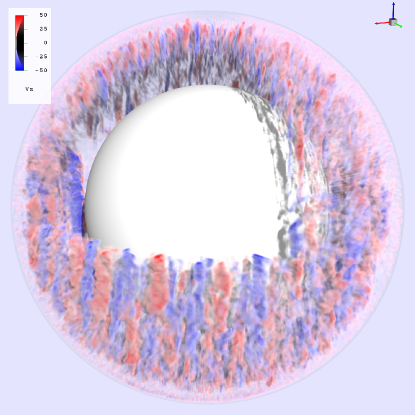
Figure 2: Radial velocity component of a characteristic EULAG-MHD simulation of rotating convection. The elongated convective rolls are the so-called banana cells, typical from rotationally constrained motions.

Although this approach has been instrumental to obtain mean-flows and cyclic dynamos resembling the observations, it still has some issues that must be addressed. For instance, Guerrero et al. (2013) used EULAG-MHD to study how mean-flows develop and sustain in simulated stars rotating at different rates. Their reference simulations have $128\times 64\times 64$ grid points in the $\varphi$, $\theta$ and $r$ directions, respectively. Rotating at the solar rotation rate it develops solar-like DR. When the resolution is doubled or increased four fold, the resulting DR exhibits different patterns. Thus, understanding the interplay between a scale independent Newtonian cooling and the implicit numerical dissipation (depending on numerical resolution) is necessary.

3 Mean flows

Differential rotation and meridional circulation (MC) are stellar large scale motions in the longitudinal and the meridional directions, respectively. Thanks to helioseismology, the differential rotation in the Sun has been measured with great accuracy (Schou et al., 1998). The profile shown in Fig. 1 (bottom-left panel) is a long term average of the angular velocity. Its main characteristics are: fast equator, slow poles with conical isocontours. Latitudinal differential rotation goes from the surface down to the tachocline at $\sim 0.71R_{\odot}$, from where the rotation is rigid. At the surface there is a thin layer of negative shear called the near-surface shear layer (NSSL). The solar DR suffers periodic speeds-up and slows-down called torsional oscillations (e.g., Howard & Labonte, 1980; Kosovichev & Schou, 1997; Antia & Basu, 2001; Vorontsov et al., 2002).

The meridional circulation, observed in the solar photosphere with different techniques, shows poleward flows on each hemisphere. Its amplitude of, about $20$ m s^-1, also fluctuates with the solar cycle. The helioseismic signal of the meridional flow from the solar interior is weak. For that reason, despite that few attempts have been conducted, its profile has not yet been accurately measured. Zhao et al. (2013); Schad et al. (2013); Böning et al. (2017) inferred meridional circulation patterns with multiple radial cells. Liang et al. (2018) reported evidences for single cell circulation.

Global simulations aim to reproduce the observed properties of these mean-flows. However, explaining their peculiarities is still challenging. Simulations from diverse numerical techniques and codes have consistently found a transition from anti-solar DR (with slow equator and fast poles) for slow rotating models, to solar-like DR for rotationally constrained turbulent convection (Gilman, 1977; Käpylä et al., 2011; Guerrero et al., 2013; Gastine et al., 2014). This transition seems to occur when the Rossby number, measuring the ratio between the rotational period and the convective turnover time ($\mbox{\rm Ro}=P_{\rm rot}/\tau_{c}$), is about one. This point marks the transition between strong and fast convection and slow convective motions influenced by the Coriolis force. Self consistently developed tachoclines have been found in recent simulations (e.g., Guerrero et al., 2013; Brun et al., 2017). Similarly, the formation of the NSSL has been studied in recent papers (Matilsky et al., 2019).

From the simulation results it is possible to explore how this flows are sustained. Differential rotation may be explained from the distribution of angular momentum ${\cal L}=\rho\varpi\overline{u}_{\varphi}$, where $\overline{u}_{\varphi}$ is the mean, longitudinally averaged, zonal flow and $\varpi=r\sin\theta$ is the lever arm. In the HD case its evolution equation is

$$\frac{\partial{\cal L}}{\partial t}=-\nabla\cdot\left(\varpi\left[\rho(\overline{u}_{\varphi}+\varpi\Omega_{0})\overline{\bm{u}}_{\rm m}+\rho\overline{u_{\varphi}^{\prime}{\bm{u}}^{\prime}_{\rm m}}\right]\right),$$ (7)

where, $\overline{\bm{u}}_{\rm m}$, ${\bm{u}}^{\prime}_{\rm m}$ are the mean and turbulent meridional ($r$ and $\theta$) components of the velocity field, respectively. All these terms can be computed from the global simulations. For solar-like differential rotation, the second term on the RHS, namely the Reynolds stresses, dominate over the meridional circulation terms, first term on the RHS. A mostly positive latitudinal Reynolds stress component, $\rho\varpi\overline{{u}_{\phi}^{\prime}{u}^{\prime}_{\theta}}$, transporting angular momentum towards the equator, is a robust feature of global simulations of the Sun (Brun & Toomre, 2002; Guerrero et al., 2013; Featherstone & Miesch, 2015; Passos et al., 2017). This result is in agreement with the $\Lambda$-effect theory (Ruediger, 1989) where the Reynold stresses are parametrized as $R_{ij}=R_{ij}^{\Lambda}+R_{ij}^{\nu}$. Here, the first and second terms correspond to non-diffusive and diffusive parts of the $\Lambda$-effect, respectively. Positive values of the non diffusive part are required to sustain solar-like DR (Kitchatinov, 2013).

For anti-solar DR the meridional circulation terms dominate, advecting angular momentum towards higher latitudes. Featherstone & Miesch (2015) argue that this meridional flow is driven by the transport of angular momentum through the so-called gyroscopic pumping mechanism which results from Eq. (7) and considering steady state ($\partial{\cal L}/\partial t=0$). Under this scenario, negative values of $-\nabla\cdot\varpi\rho\overline{u_{\varphi}^{\prime}{\bm{u}}^{\prime}_{\rm m}}$ will induce a strong meridional flow away from the rotation axis at lower latitudes. Because of the closed boundary conditions, this flow transports angular momentum to the high latitudes increasing the angular velocity. At the equator it will result in a differential rotation that decreases away from the rotation axis (Miesch & Hindman, 2011).

This description is completed with the equation of the thermal wind balance (TWB) which in its HD form reads,

$$\varpi\frac{\partial\overline{\Omega}^{2}}{\partial z}=\frac{g}{r}\frac{\partial}{\partial\theta}\left(\frac{\Theta^{\prime}}{\Theta_{0}}\right)\;,$$ (8)

where $z$ is the height in cylindrical coordinates. If the DR has isocontours which are not aligned with the rotation axis, the term on the LHS implies gyroscopic pumping. The term on the RHS is the baroclinicity of the system. Models with anti-solar differential rotation result in warm equator and cold poles, favoring then a counterclockwise meridional in the northern hemisphere. cell (Featherstone & Miesch, 2015). The same, gyroscopic pumping mechanism might explain the, more complex, multi cell pattern of MC typical of simulations with solar-like differential rotation (Guerrero et al., 2016b).

An alternative explanation to the gyroscopic pumping dominance in defining the meridional circulations comes from the $\Lambda$-effect theory. Mean-field models under this approximation explain MC from departures of the TWB (Eq. 8). Since the TWB is likely lost at the boundaries of the convection zone, viscous forces might drive the meridional flows (Kitchatinov, 2013). In contrast with global simulations where all the driving forces arise naturally, in $\Lambda$-effect mean-field simulations these forces are parametrized by theoretical turbulence models. Thus, including this viscous force in the equation for the vorticity results in single circulation cells for both fast and slow rotating stars (Karak et al., 2014). This disagrees with the results of HD global simulations where single cell circulation is obtained for slow rotation and multiple cells show up in fast rotation simulations. (See, however, Pipin & Kosovichev (2018) for $\Lambda$-effect mean-field simulations with double cell MC.)

In the MHD case, simulations have shown that the magnetic field quenches the convective flux affecting the distribution of the Reynolds stresses and, therefore, of angular momentum. It allows for slow rotating models to develop solar-like DR (Fan & Fang, 2014; Karak et al., 2015; Guerrero et al., 2019b). The HD and MHD balance of angular momentum and thermal wind for solar-like DR are discussed in detail by Passos et al. (2017). The transition from solar-like to anti-solar DR for HD and MHD simulations was explored by Karak et al. (2015). It was found that the transition is smooth for dynamo simulations and occurs at larger values of the Rossby number. In the EULAG-MHD simulations presented in Guerrero et al. (2019b) this transition is not observed for Rossby numbers up to $\sim 3$ ($63$ days rotational period). This can be seen in Fig. 3 depicting the DR (left of each panel) and MC (right) of some simulations in that publication. Note also that in all the cases the MC has multiple cells in radius at lower latitudes.

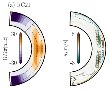
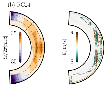
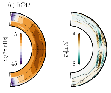
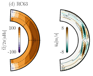
Figure 3: Differential rotation in the inertial frame, $\overline{\Omega}-\Omega_{0}$, and meridional circulation of characteristic simulations of Guerrero et al. (2019b). In the differential rotation panels the color contours show regions of iso-rotation. In the meridional circulation panels the continuous (dashed) lines represent clockwise (counterclockwise) circulation. The color contours show the mean latitudinal velocity, $\overline{u}_{\theta}$. Adapted from Guerrero et al. (2019b).

Differential rotation has been observed in other stars by different means including tracking magnetic features, photometric variability and asteroseismology (e.g., Reinhold & Gizon, 2015; Kővári et al., 2017; Benomar et al., 2018). The results indicate DR consistent with faster equator for a large number of observed stars. Anti-solar DR has not been yet confirmed. Reinhold & Gizon (2015); Kővári et al. (2017) found a shear parameter, $\alpha^{*}=\Delta\Omega/\Omega_{\rm eq}$, increasing with the rotational period of the stars with values between $10^{-3}$ and $0.5$. The recent asteroseismology analysis of Benomar et al. (2018) does not show a clear defined trend and found shear values larger than unity. In the Sun $\Delta\Omega/\Omega_{\rm eq}$, with $\Delta\Omega=\Omega_{\rm eq}-\Omega_{45}$, is about $0.1$.

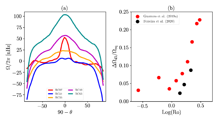
Figure 4: (a) Latitudinal differential rotation in the inertial frame, $\overline{\Omega}-\Omega_{0}$, of the simulations presented in Guerrero et al. (2019b); (b) relative shear, $\Delta\Omega/\Omega_{\rm eq}$, where $\Delta\Omega=\Omega_{\rm eq}-\Omega_{45}$, as a function of the Rossby number (in logarithmic scale). The red and black dots correspond to the simulations of Guerrero et al. (2019b) and Ferreira et al. (2020), respectively.

Most of the observational findings on DR estimate the shear parameter by assuming a solar-like latitudinal variation, i.e., $\sim\cos^{2}\theta$. This, however, might not be the case. Figure 4 shows the results of the global simulations presented in Guerrero et al. (2019b). The LHS panel shows the latitudinal profile of $\overline{\Omega}$ in the inertial frame. It is evident that the latitudinal shear has different profiles for different rotational periods. The fast rotating simulations show strong variation concentrated at the equator and the poles. Intermediate cases have smooth profiles while slow rotating simulations develop a strong shear between the equator and the poles. The parameter $\alpha^{*}$, measuring the shear between the equator and $45^{\circ}$ (to compare with astroseismic results of Benomar et al., 2018), as a function of the Rossby number is presented on the RHS of Fig. 4. The shear evidently increases with the increase of Ro (decreasing rotation). The black dots, corresponding to simulations of the star HD43587 presented in Ferreira et al. (2020), follow a similar trend yet with smaller values of $\alpha^{*}$. If the increase of the shear with the rotational period is confirmed by further observations, the physics behind this counterintuitive result must be elucidated through global models.

4 Large-scale magnetic field

4.1 The solar dynamo

For the reasons discussed in previous sections, performing global MHD simulation of the solar dynamo, including all the features of the convection zone, and all the relevant scales involved in the processes, is still unfeasible. Nevertheless, in view of the ambiguities of the mean-field simulations, global MHD modeling is perhaps the most promising method to understand the dynamo mechanism in stellar interiors. Several attempts have been done over the last decades with the aim of capturing some relevant physics. In the solar context, Gilman & Miller (1981); Gilman (1983) presented pseudo-spectral simulations of rotating convection in the Boussinesq approximation. They were able to obtain dynamo action and even magnetic field reversals. The anelastic approximation was used in the early works of Glatzmaier (1984, 1985a, 1985b). With the advent of parallel supercomputer architectures, simulations with improved resolutions were performed by Brun et al. (2004) with the ASH code. They obtained amplification of the magnetic field without a large-scale dynamo.

Large-scale organized magnetic fields were found in the simulations performed by Browning et al. (2006). They achieve mean-field dynamo action by forcing a shear layer, i.e., mimicking the tachocline, below the convection zone. Nevertheless, Brown et al. (2010) showed that the formation of organized global structures do not need strong tachocline shear but only rapidly rotating turbulent convection. Their simulations, rotating $\sim 3$ times faster than the Sun, developed steady antisymmetric magnetic wreaths.

Periodic magnetic fields were first reported by Ghizaru et al. (2010) with the ILES formulation of the EULAG-MHD code. The lower values of the numerical viscosity due to the implicit SGS scheme, together with the energy description presented in §6 led to a self-consistent development of the tachocline and a solar-like differential rotation. The resulting dynamo mode does not show, however, clear latitudinal migration and reverses with a cycle period of 30 yrs.

Fully compressible simulations of spherical wedges performed with the pencil-code also found cyclic dynamo solutions (Käpylä et al., 2010). Also, Käpylä et al. (2012) reported solutions where the toroidal magnetic field migrates towards the equator resembling the solar observations. Considering slope-limited diffusion for diffusing momentum, and eddy values for the heat transport coefficients and the magnetic diffusivity, Augustson et al. (2015) obtained periodic field reversals with the ASH code. These cases simulate only in the convection zone and the cycle periods are between 3 to 6 yrs.

Masada et al. (2013), with a code based on second order finite differences and using the Yin-Yang grid explored the role of penetrative convection in models with and without a fraction of the radiative interior. They found that larger magnetic fields develop when the stable layer is present. Nevertheless, there is not a well defined tachocline in their results. Guerrero et al. (2016a) performed the same comparison with EULAG-MHD and explored simulations with rotation rates of $2\Omega_{\odot}$, $\Omega_{\odot}$ and $\Omega_{\odot}/2$. The results showed striking differences between the two cases. While the resulting latitudinal shear was roughly the same, the presence of the radial shear at the tachoclines led to a different behavior of the strong magnetic field developed at and below these shear regions. As a consequence, the cycle period, of about 2 yrs in simulations of the convection zone only, resulted of the order of decades.

Figure 5 shows the time-latitude butterfly diagram of a recent EULAG-MHD simulation of the solar analog HD43587 presented in Ferreira et al. (2020). The color contours represent the strength of the mean toroidal field, $\overline{B}_{\phi}$. The continuous (dashed) contour lines show the positive (negative) levels of the mean radial magnetic field, $\overline{B}_{r}$. The panels (a), (b) and (c) correspond to different depths, as indicated. At $0.85R_{*}$, where $R_{*}=1.19R_{\odot}$ is the radius of the star, the butterfly diagram shows qualitative similarities with the solar one, i.e., there is strong magnetic field migrating equatorward at lower latitudes and poleward migration at higher latitudes. This configuration is likely the result of magnetic field emerging from the tacholine at lower latitudes, (see also the upper-left panel of Fig. 5 which shows a snapshot of the magnetic field configuration in the meridional, $\theta-r$, plane), followed by poleward advection at the upper part of the domain. At $0.95R_{*}$, upper boundary of the simulation, only the polar branch is evident (this stage corresponds to the lower-left panel of Fig. 5).

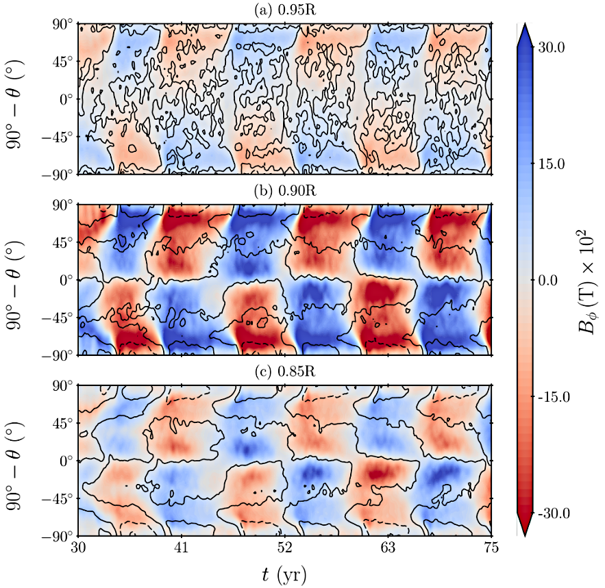
Figure 5: Time-latitude butterfly diagram of one simulation of the star HD43587. The color contours show the toroidal mean magnetic field, $\overline{B}_{\phi}$. The continuous (dashed) contour lines show the positive (negative) mean radial magnetic field, $\overline{B}_{r}$.

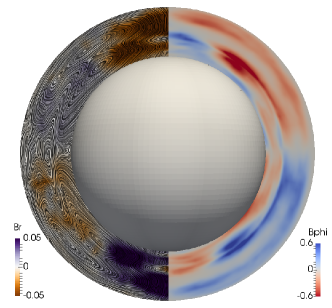
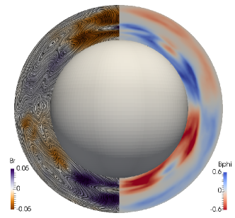
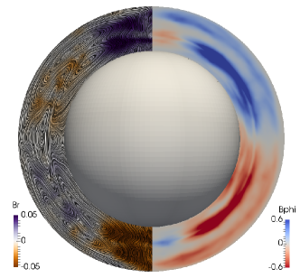
Figure 6: Snapshots presenting half magnetic cycle in the EULAG-MHD simulation P25 presented in Ferreira et al. (2020). On the left of each snapshot, the LIC representation depicts the distribution of the poloidal field lines with the color indicating the magnitude of the mean radial field, $\bar{B}_{r}(t,\theta,r)$. The colored contours on the right quadrants correspond to the azimuthal mean magnetic field, $\bar{B}_{\varphi}(t,\theta,r)$.

4.2 Mean-field interpretation

Similar to the theory of the $\Lambda$-effect, a mean-field model can be used to describe the evolution of the large-scale magnetic field, $\overline{{\bm{B}}}$ in stellar interiors (Parker, 1955; Steenbeck et al., 1966). After separation of the turbulent and the large scales, the induction equation (Eq. 4) becomes,

$$\frac{\partial\overline{\bm{B}}}{\partial t}=\nabla\times(\overline{\bm{u}}\times\overline{\bm{B}})+\nabla\times(\alpha\overline{\bm{B}})-\nabla\times(\eta\nabla\times\overline{\bm{B}}),$$ (9)

where $\overline{\bm{B}}=(\overline{B}_{r},\overline{B}_{\theta},\overline{B}_{\phi})$ and $\overline{\bm{u}}=(\overline{u}_{r},\overline{u}_{\theta},\overline{u}_{\phi})$ are the averaged magnetic and velocity fields. In the second term on the RHS, the $\alpha$ term stems for the $\alpha$-effect which has kinetic and magnetic contributions, namely $\alpha=\alpha_{\rm k}+\alpha_{\rm m}$. These terms are the first order correlations of the turbulent electromotive force,

$$\overline{\cal{\bm{E}}}=\overline{{\bm{u}}^{\prime}\times{\bm{B}}^{\prime}}\simeq\alpha\overline{\bm{B}}-\eta_{\rm t}\mu_{0}\nabla\times\overline{\bm{B}}\;,$$ (10)

where ${\bm{u}}^{\prime}$ and ${\bm{B}}^{\prime}$ are the turbulent velocity and magnetic fields and $\eta_{\rm t}$ is the turbulent magnetic diffusivity. The $\alpha$ terms induce the large-scale magnetic field from small scale helical motions and currents. Under suitable closure models (e.g., Pouquet et al., 1976; Moffatt, 1978), the it may be expressed as:

$$\alpha=\alpha_{\rm k}+\alpha_{\rm m}=-\frac{\tau_{c}}{3}\langle{\bm{\omega}^{\prime}}\cdot{\bm{u}^{\prime}}\rangle+\frac{\tau_{c}}{3}\langle{\bm{j}^{\prime}}\cdot{\bm{B}^{\prime}}\rangle/\rho\;,$$ (11)

where ${\bm{\omega}}^{\prime}=\nabla\times{\bm{u}}^{\prime}$ and ${\bm{j}}^{\prime}=\nabla\times{\bm{B}}^{\prime}$ are the small scale vorticity and current, respectively, and $\tau_{c}$ is the convective turnover time of the turbulent motions.

In the third term in Eq. (9), $\eta=\eta_{m}+\eta_{\rm t}$ is the sum of the molecular and the turbulent magnetic diffusivities. The turbulent contribution is dominant by several orders of magnitude and under the first order smoothed approximation (FOSA) may be computed as

$$\eta_{\rm t}=\frac{1}{3}\tau_{c}u^{\prime 2}\;.$$ (12)

Either the terms in the electromotive force (Eq. 10) or those in Eqs. (11 and 12) may be estimated from the global simulations output allowing to search for a theoretical interpretation of complex results. This has been done for the EULAG-MHD simulations of Ghizaru et al. (2010) by using a method for multidimensional regression (Racine et al., 2011). Their results indicate that the process is consistent with an $\alpha^{2}\Omega$ dynamo (see also Simard et al., 2013). For pencil-code dynamo results Warnecke et al. (2014) computed the dynamo coefficients, $\alpha$ and $\Omega$, and proved that the evolution of the magnetic field follows the Parker (1955)-Yoshimura (1975) sign rule. More recently Warnecke et al. (2018) used the test-field method (Schrinner et al., 2005; Brandenburg et al., 2008) to perform a fiducial prediction of the electromotive force coefficients. For the profiles and amplitude of the coefficients, they conclude that the dominant dynamo in pencil-code simulations is of $\alpha\Omega$ type with a localized $\alpha^{2}$ dynamo.

The FOSA coefficients of Eqs. (11 and 12) were computed by Guerrero et al. (2019b) for EULAG-MHD simulations including both, radiative and a convective layer; having solar-like ambient state and rotating at different rates. The results showed that for fast rotation the dominant dynamo is of $\alpha\Omega$ type and operates at the convection zone (Fig. 7(a)). For intermediate and slow rotation rates, the dominant dynamo operates locally at the tachocline and is of $\alpha^{2}\Omega$ type (Fig. 7(b and c)). The $\alpha$-effect contributes to the amplification of the toroidal field at intermediate to high latitudes while the rotational shear generates toroidal field at the equator. The results indicated that the appearance of cycles in tachocline dynamos is related to the strength of the equatorial shear. The most striking result observed in the simulations is that the $\alpha$-effect, at and below the tachocline, has magnetic origin, i.e., the inductive contribution of small-scale current helicity (second term in Eq. 11) is dominant over the induction of magnetic field by small-scale helical eddies.

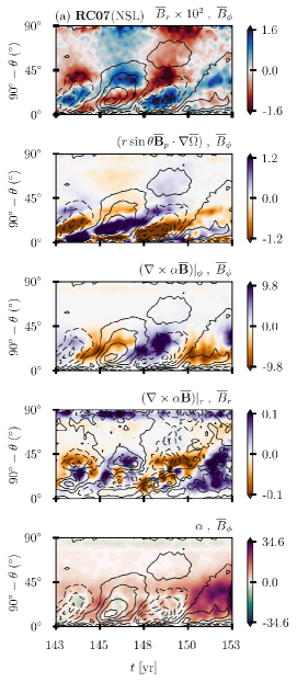
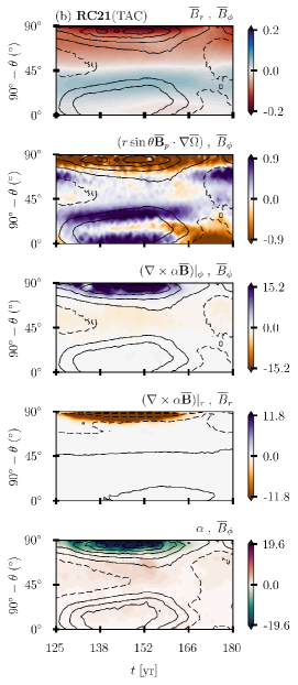
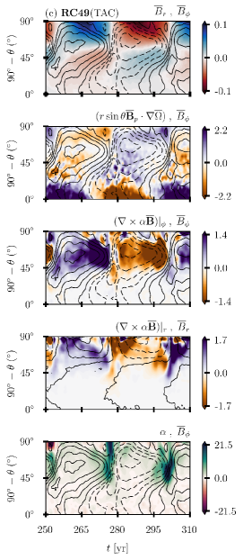
Figure 7: Mean-field sources of large-scale magnetic fields in some characteristic simulations presented in Guerrero et al. (2019b). The columns correspond to simulations with a cycle period of 7 (a), 21 (b) and 49 (c) days, respectively. All the quantities are averaged in longitude and over a radial extent in the near-surface layer (a) or in the tachocline (b and c). From top to bottom the panels display the radial, $\bar{B}_{r}$ (colored contours) and toroidal, $\bar{B}_{\phi}$ (contour lines) mean magnetic fields; the sources of the toroidal field, $r\sin\theta(\bar{B}_{p}\cdot\nabla)\bar{\Omega}$ and $(\nabla\times\alpha\bar{\bf B})|_{\phi}$ (colored contours), both compared with $\bar{B}_{\phi}$; the source of the radial field, $(\nabla\times\alpha\bar{\bf B})|_{r}$ (color), compared with $\bar{B}_{r}$ (contour lines); and $\alpha=\alpha_{k}+\alpha_{m}$ (colored contours), compared with $\bar{B}_{\phi}$. In the color map the dimensions are [T] for the magnetic field, $10^{-8}$ [T/s] for the source terms, and [m/s] for the $\alpha$-effect, respectively. Adapted from Guerrero et al. (2019b).

The magnetic loop observed in the deep seated $\alpha^{2}\Omega$ dynamos described above is illustrated in Fig. 8. Turbulent convection is necessary to generate and sustain the differential rotation (left panel). It supplies the strong shear necessary for the $\Omega$-effect to develop a large-scale toroidal magnetic field, $\overline{B}_{\phi}$ (top). The generated layer of toroidal field is unstable to the shear present in the region and decays in non-axisymmetric modes ($m\neq 0$), whose collective contribution, in turn, develop an axisymmetric magnetic $\alpha$-effect (right). This $\alpha$-effect contributes to the generation of both, toroidal and poloidal mean magnetic fields. Between maxima and minima the developed magnetic tension speeds-up and slows-down the azimuthal motions creating a pattern of torsional oscillations. The mechanism generating this pattern is described in detail in Guerrero et al. (2016b).

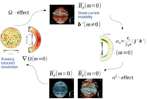
Figure 8: Dynamo loop for oscillatory $\alpha^{2}\Omega$ dynamos operating in the simulations of Guerrero et al. (2019b).

Several instabilities are simultaneously operating in the cycle depicted in Fig. 8. Disentangle them is a rather difficult task, thus, simple simulations are necessary to understand the processes separately. The most intriguing mechanism in this dynamo is perhaps the generation of small scale helicities in the stable layer because of instabilities of the magnetic field. We have claimed that it is consistent with a shear-current instability where a decaying toroidal field produces helical currents that allow the growing of the poloidal field. This kind of instabilities was first proposed by (Tayler, 1973) and studied further by several authors (e.g., Pitts & Tayler, 1985; Bonanno & Urpin, 2012, 2013). In the presence of shear the instability was explored in detail by Cally (2003); Miesch et al. (2007). They reported that the shear-current instability for a broad band of toroidal magnetic field results in modes where the field lines open in the form of a clamshell. When the initial field has two bands of opposite polarity, the axis of the bands tilts in latitude. Similarly to the Tayler instability, in these cases the fastest growing mode is $m=1$. The clamshell instability is observed in the simulations presented in (Guerrero et al., 2019b, see their Fig. 10). A cyclic dynamo based on Tayler-like instabilities has been previously proposed by Spruit (2002); Zahn et al. (2007); Bonanno (2013), however, the global EULAG-MHD simulations of Guerrero et al. (2019b) were the first ones to develop and sustain the dynamo.

To fully understand how these instabilities are the source of an $\alpha$-effect, Guerrero et al. (2019b) explored the stabilizing properties of gravity to the Tayler instability using the EULAG-MHD code. The results showed that for weak gravitational stratification the instability has radial dependence, while for larger stratification the unstable modes develop in horizontal layers and might have oscillatory behavior. The growth rate depends on the local value of the Brunt-Väisäla (BV) frequency (in turn depending on the gravity force). An extension to this work is currently being carried out including rotation and shear (Monteiro et al. 2020, in preparation).

4.3 Stellar cycles

The study of magnetism in stars different from the Sun is necessary to get a broad understanding of the physics in stellar interiors as well as the interaction between stars and planetary systems. It may also provide hints and constraints to unveil the details of the solar dynamo. From the Mount Wilson data several stars were found to have activity cycles (Baliunas et al., 1995; Saar & Brandenburg, 1999) evident in the ${\rm Ca}\leavevmode\nobreak\ _{\rm II}\;{\rm H}$ and ${\rm K}$ spectral lines. Further studies correlated the magnetic cycle period to the rotational period (Noyes et al., 1984; Brandenburg et al., 1998; Böhm-Vitense, 2007; Brandenburg et al., 2017). Two main branches, classified as active (A) or inactive (I) depending also in the strength of the magnetic field, have been canonically discussed in the literature (Brandenburg et al., 1998; Böhm-Vitense, 2007; Brandenburg et al., 2017). Both of them show a positive linear correlation between $P_{\rm cyc}$ and $P_{\rm rot}$. The same two branches appear parallel when $\log(P_{\rm rot}/P_{\rm cyc})$ is compared with $\log\langle R^{\prime}_{HK}\rangle$, where $\langle R^{\prime}_{HK}\rangle=F^{\prime}_{HK}/F_{\rm bol}$ is the mean fractional ${\rm Ca}\leavevmode\nobreak\ _{\rm II}\;{\rm H}$ and ${\rm K}$ flux normalized with the stellar bolometric flux, $F_{\rm bol}$ (Brandenburg et al., 1998, 2017). Olspert et al. (2018) re-visited the Mount Wilson data computing cycle periods with sophisticated techniques for analysis of periodic and quasi-periodic time series. Their results confirmed the existence of the two branches, A and I. They found, however, that the trend of the active branch is not positive but broadly distributed and connects with a third transitional branch of activity (Lehtinen et al., 2016).

Over the last years few attempts have been done to explore the relation between magnetic cycles and rotation by using global convective dynamo simulations. Strugarek et al. (2017) performed ILES simulations with the EULAG-MHD code. They found a negative correlation between $P_{\rm cyc}$ and $P_{\rm rot}$ and argue that the cycle period is established by the back-reaction of the magnetic field over the differential rotation (Strugarek et al., 2018). Warnecke (2018) reported a similar relation in pencil-code wedge simulations. They attributed, however, the magnetic cycles to $\alpha\Omega$ dynamos operating at the base of the convection zone. The resulting cycle periods follow the linear mean-field dynamo theory (see e.g., Stix, 1976):

$$P_{\rm cyc}\propto(C_{\alpha}C_{\Omega})^{-1/2}\;,$$ (13)

where $C_{\alpha}$ and $C_{\Omega}$ are non-dimensional quantities comparing the inductive effects of the $\alpha$ and the $\Omega$ effects, respectively, with the magnetic turbulent diffusion. Warnecke (2018) argues that their simulations are reproducing the transitional branch. Another set of simulations performed with the pencil-code cover the entire domain in the $\varphi$ direction but without reaching the poles (Viviani et al., 2018). They explore fast convective dynamos with rotations from $1$ to $30$ $\Omega_{\odot}$. Since rotation breaks the convective cells, these simulations require high resolution. They found that the slow rotating cases fall in the I branch but having a negative tilt. On the other hand, the fast rotating cases result in non-axisymmetric dynamos with cycles falling in a different branch of activity representative of superactive stars.

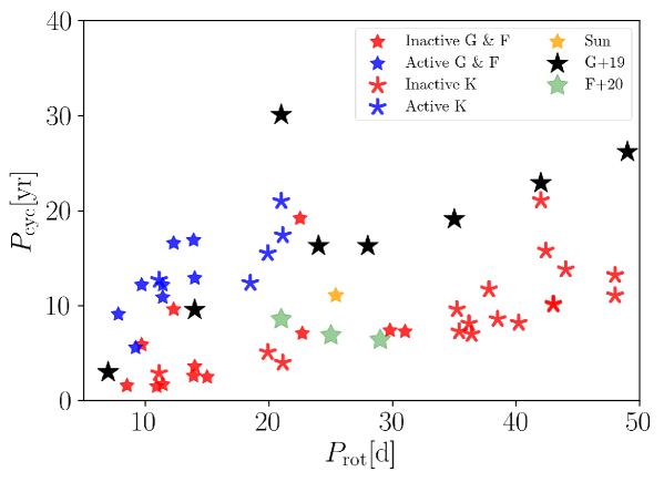
Figure 9: Magnetic cycle period of rotation, $P_{\rm cyc}$ as a function of the rotational period $P_{\rm rot}$. The black stars correspond to the simulations presented in Guerrero et al. (2019b), the green stars correspond to the simulations of the star HD43586 presented in Ferreira et al. (2020).

All these cyclic dynamo simulations have in common the absence of the strong shear at the tachocline. Guerrero et al. (2016a) found that long-lived strong magnetic fields develop in models that include the tachocline and a stable layer underneath. A longer set of simulations was recently presented in Guerrero et al. (2019b) with dynamo solutions for rotational periods between 7 and 63 days. The results revealed two different types of dynamos: $\alpha\Omega$ dynamos operating at the bulk of the convection zone for fast rotating simulations, and depth seated $\alpha^{2}\Omega$ dynamos for intermediate and slow rotating simulations. In between, there is a bifurcation point where deep seated oscillatory dynamo at lower latitudes coexists with a steady dynamo at the poles. This point marks the level of equatorial shear necessary to generate tachocline cyclic dynamos. In both types of dynamos $P_{\rm cyc}$ increases with $P_{\rm rot}$. The ones operating in the convection zone fall close to the active branch whereas the tachocline dynamos fall in between the two branches (see black stars in Fig. 9). Although the deep seated magnetic cycles are consistent with $\alpha^{2}\Omega$ dynamos (as seen in §4.2), the cycle periods do not agree with the mean-field prediction (Eq. 13). The cycle is established once a balance between a non-linear dynamo and tachocline instabilities is reached. A better understanding of this mechanism is necessary to be able of predicting cycle lengths as a function of stellar parameters. Furthermore, the numerical experiments presented in Ferreira et al. (2020) show that the simulations are rather sensitive to the profile o the ambient state, $\Theta_{\rm amb}$, described in section §2.3.

In one hand, the level of superadiabaticity of the convection zone determines the strength of the convection, and therefore the profile of differential rotation. On the other hand, the level of subadiabaticity in the stable layer determines the Brunt-Väisäla frequency and therefore the development of gravity waves in the stable layer. These waves might be fundamental for the development of the instability of toroidal fields in radiative zones (Guerrero et al., 2019a). We have implemented these ideas in the simulations of the solar analog HD43568 (Ferreira et al., 2020). The stratification profile in the convection zone is set to fit the convective velocity obtained by the mixing length theory (MLT); in the stable layer it fits the BV frequency of the same structural model. In addition, we changed the magnetic boundary condition at the bottom of the domain from radial field to perfect conductor. The results agree with the spectroscopic analysis indicating an activity cycle of $\sim 10$ years and low magnetic activity levels. Simulations for 21, 25 and 29 days results in cycles which fall in the inactive branch (see green stars in Fig. 9). Further simulations with this improved ambient state configuration are currently being performed for the Sun and other stars of the Mount Wilson sample.

5 Conclusions

In this work we described the modeling of solar and stellar dynamos through self-consistent global simulations. We argue that these are the most relevant tools to understand the development and sustain of stellar magnetic fields. Special focus is given to the recent ILES simulations performed with the anelastic solver EULAG-MHD. A short discussion on the need of including SGS modeling in the current global modeling was also presented.

In spite of the recent advances, the current models still are unable to reproduce the main characteristics of the solar dynamo nor the empirical relations between magnetic cycle periods and magnetic field strength with stellar parameters like the Rossby number. It is worth mentioning, however, that these relations still need to be revised with a large number of samples and longer observational missions.

Regarding the development of mean flows, the result of global simulations with different numerical schemes show good agreement. Consequently, great advances have been done in the understanding of the buildup of these flows. While the role of the Reynolds stresses is unanimously recognized as the responsible for the sustain of the differential rotation, the formation of meridional circulation has not yet a closed theoretical interpretation. It is attributed to the gyroscopic pumping mechanism resulting from the thermal wind balance (Miesch & Hindman, 2011), or to deviations of this equilibrium given mostly by viscous forcing at boundary layers (Kitchatinov, 2013). Most of global models tend to support the first alternative (e.g., Featherstone & Miesch, 2015; Guerrero et al., 2016b).

With respect to the development of mean magnetic fields, several questions still remain to be answered. Perhaps the most important are, first, what global simulations have missed until now to reproduce solar-like patterns? Second, what physical processes are occurring in the global simulations? And third, how relevant are the tachoclines in the dynamo process? About the first question, there is still room for exploration. For instance, the role of the stratification, compressibility and a realistic upper magnetic boundary are yet to be studied. In addition, simulations with higher Reynolds numbers would likely be possible over the starting decade. With respect to the second question, the work until now has proven that the FOSA approximation might allow to distinguish what type of dynamo is occurring. However, computing the full set of elements in the electromotive force tensors seems to be the appropriate alternative to fully understand the dynamo process (e.g., Warnecke et al., 2018). The third question has been an issue of debate over the last years. Doubts about the relevance of the layers of strong radial shear started from the observational results of Wright & Drake (2016). They reported that stars without tachoclines follow the same scaling law between the magnetic field strength and Ro that stars with this layer. On the other hand, recent observations of the magnetic field topology in solar-type stars with different ages, show a clear change at the age of the formation of the radiative zone (Gregory et al., 2012). The structural change corresponds to the shift from a mainly poloidal configuration to a magnetic field dominated by high order modes. This is a clear indication of a change in the dynamo regime at the age when the tachoclines appear. Whatever is the case, for the time being global models with and without tachoclines are able to develop large-scale magnetic fields with polarity reversals. As these models are better understood, further observational evidence will provide a clearest scenario of stellar magnetism.

BrandenburgThe cycle to rotation frequency is found to increase with stellar activity. Do you agree that there is currently no model that reproduces this? How can we hope to reproduce the Sun if this essential feature is not reproduced. Could you speculate what might be missing in the models?

GuerreroAs a matter of fact no current model reproduces this relation. Nevertheless, cycle dynamos in global simulations are relatively new. There is still a broad parameter space to explore in the simulations, specially concerning the resolution and the energy transport issue. I’m optimistic that as soon as these issues are clarified the models will be able to reproduce better the solar and stellar magnetism. Note also that observations are still providing new results.

StrugarekThe trend of differential rotation seems to increase as rotation rate diminishes. This is at odds with other 3D simulations with and without underlying stable layer. How is differential rotation sustained in your models?

GuerreroThe latitudinal shear indeed increases when the rotational rate decreases. This relation, not included in the presentation, is shown in Fig. 4 of this proceeding. The results, however, are not completely at odds with other simulations. See, for instance, the results presented in Gastine et al. (2014) including global simulations from several groups. As rotation decreases the shear increases before changing sing for anti-solar differential rotation. In Guerrero et al. (2016b) we presented the angular momentum balance of one particular simulation, a detailed analysis of all the simulations is still on its way. This will clarify the reason for this relation.

LuhmannThere is a well-known observed relationship between surface polar fields and cycle size. Do the simulations reveal a physical reason for that relationship?

GuerreroThis property has not yet been studied in the results of global models. The reason is that unfortunately there is not yet a model reproducing well all the properties of the solar cycle.