Longitudinal fluid response and pseudorapidity dependent flow in relativistic heavy-ion collisions

Abstract

We study the pseudorapidity dependent hydrodynamic response in heavy-ion collisions. A differential hydrodynamic relation is obtained for elliptic flow. Using event-by-event simulations of 3+1D MUSIC, with initial conditions generated via a multi-phase transport (AMPT) model, the differential response relation is verified. Based on the response relation, we find that the two-point correlation of elliptic flow in pseudorapidity are separated into the fluid response and the two-point correlation of initial eccentricity.

1 Introduction

The fluidity of the quark-gluon plasma (QGP) created in heavy-ion collisions has been discovered through the measurements of flow harmonics in multi-particle correlations. These flow harmonics can be understood as the fluid response to the decomposed azimuthal modes associated with the initial state geometrical deformations. For instance, it is noticed that the eccentricity of the initial density profile, $\mathcal{E}_{2}$, is linear to the elliptic flow $V_{2}$ [1]. While this linear relation has been well studied by relativistic hydrodynamics [2, 3, 4], a pseudorapidity dependent hydrodynamic response relation between $V_{2}$ and $\mathcal{E}_{2}$ is absent in the community, until some recent studies [5, 6]. In the current proceeding, we generalize the linear response relation for the second flow harmonics, to a pseudorapidity dependent hydrodynamic response. With event-by-event simulations of 3+1D MUSIC with respect to initial condition from AMPT, the pseudorapidity dependent response relation is confirmed. Given the pseudorapidity dependent hydrodynamic response, we are able to explore the relation between the two-point correlation of elliptic flow in pseudorapidity and that of initial eccentricity.

2 Framework

To study the pseudorapidity dependent hydrodynamic response, we generalize the linear response relation as

$$V_{2}(\zeta)=\int_{-\infty}^{\infty}d\xi\;G(\zeta-\xi)\mathcal{E}_{2}(\xi)\,,$$ (1)

where $\zeta$ is the pseudorapidity and $\xi$ is the space-time rapidity. Although the response function $G(\zeta-\xi)$ implies a boost invariant background, the broken boost invariant symmetry in realistic heavy-ion collisions can be accounted for by perturbations. In Eq. (1), the pseudorapidity dependent flow is defined according to the Fourier decomposition of the particle emission probability in heavy-ion collisions, $P(\phi_{p},\zeta)$

$$P(\phi_{p},\zeta)=\frac{1}{2\pi}\sum_{n=-\infty}^{\infty}V_{n}(\zeta)e^{-in\phi_{p}}\,,\qquad{\mbox{integrated flow: }}V_{n}=\int_{-\infty}^{\infty}d\zeta V_{n}(\zeta)\,.$$ (2)

With respect to initial energy density $\rho(\vec{x}_{\perp},\xi)$, the initial eccentricity is defined as $\mathcal{E}_{2}(\xi)=-\int d^{2}\vec{x}_{\perp}\;\rho(\vec{x}_{\perp},\xi)(x+iy)^{2}/\int d\xi d^{2}\vec{x}_{\perp}\;\rho(\vec{x}_{\perp},\xi)|x+iy|^{2}\,$. Up to integration over $\xi$, one finds that $\mathcal{E}_{2}=\int_{-\infty}^{\infty}\mathcal{E}_{2}(\xi)$ is the standard eccentricity considered in literature. It is also worth mentioning that, asymptotically, $\mathcal{E}_{2}(\xi)\to 0$ when $|\xi|\to\infty$, which would allow one to ignore boundary corrections from infinities when deriving Eq. (6).

To identify the response function, it is advantageous to work through a Fourier transformation, namely, for the elliptic flow $\tilde{V}_{2}(k)=\int_{-\infty}^{\infty}d\zeta\;V_{2}(\zeta)e^{-ik\zeta}$ and initial eccentricity $\tilde{\mathcal{E}}_{2}(k)=\int_{-\infty}^{\infty}d\xi\;\mathcal{E}_{2}(\xi)e^{-ik\xi}$. In terms of the wave-number $k$, Eq. (1) becomes,

$$\tilde{V}_{2}(k)=\tilde{G}(k)\tilde{\mathcal{E}}_{2}(k)\,.$$ (3)

In the small wave number limit with $|k|\ll k^{*}$, corresponding to the hydrodynamic regime, the response function can be expanded in series of $k$. Up to the second order, the expansion is

$$\tilde{G}(k)=G_{0}+ikG_{1}-k^{2}G_{2}+O(k^{3})\,,$$ (4)

which in the $\zeta$-space amounts to

$$V_{2}(\zeta)=G_{0}\mathcal{E}_{2}(\zeta)+G_{1}\frac{d\mathcal{E}_{2}(\zeta)}{d\zeta}+G_{2}\frac{d^{2}\mathcal{E}_{2}(\zeta)}{d\zeta^{2}}+O\left(\frac{d^{3}}{d\zeta^{3}}\right)\,.$$ (5)

Note that odd order $G_{n}$ vanish owing to the parity symmetry in the background. To obtain these expansion coefficients $G_{n}$’s, we define new sets of flow variables and initial eccentricity variables weighted with powers of $\zeta$ (or $\xi$): $V^{(n)}_{2}=\int d\zeta\zeta^{n}V_{2}(\zeta)/n!\,$ and $\mathcal{E}^{(n)}_{2}=\int d\xi\xi^{n}\mathcal{E}_{2}(\xi)/n!\,.$ Using integration by parts repeatedly, with these new variables the generalized linear response relation Eq. (1) can be rewritten as

$$V_{2}^{(n)}=\sum_{i=0}^{n}(-1)^{i}G_{i}\mathcal{E}_{2}^{(n-i)}\,.$$ (6)

Note that the leading order relation $V_{2}^{(0)}=G_{0}\mathcal{E}_{2}^{(0)}$ is the familiar linear response relation of elliptic flow, with the response coefficients being calculated in event-by-event hydrodynamic simulations as [4]: $G_{0}=\left\langle V_{2}^{(0)}\mathcal{E}_{2}^{(0)*}\right\rangle\Big{/}\left\langle\mathcal{E}_{2}^{(0)}\mathcal{E}_{2}^{(0)*}\right\rangle$, where and in the following the angular brackets indicate event average. Following a similar procedure, a set of linear relations can be realized between $\mathcal{E}_{2}^{(0)}$ and $V_{2}^{(n)}-\sum_{i=0}^{n-1}(-1)^{i}G_{i}\mathcal{E}_{2}^{(n-i)}$, and $G_{n}$ can be calculated recursively. More details on these higher coefficients can be found in Ref.[5].

The pseudorapidity dependent response relation Eq. (1) is non-local, which implies that the generation of $V_{2}$ at one pseudorapidity receives contributions from other space-time rapidities. This effect can be shown in the analysis of two-point correlations. We define

$$\left\langle(\Delta\zeta)^{2}\right\rangle\equiv\frac{\int d\zeta d\zeta^{\prime}\left\langle V_{2}(\zeta)V_{2}^{*}(\zeta^{\prime})\right\rangle(\zeta^{\prime}-\zeta)^{2}}{\int d\zeta d\zeta^{\prime}\left\langle V_{2}(\zeta)V_{2}^{*}(\zeta^{\prime})\right\rangle},$$ (7)

to characterize the length of the two-point correlation measured via elliptic flow at different pseudorapidities. With the response relation derived in Eq. (6), it can be proved that

$$\left\langle(\Delta\zeta)^{2}\right\rangle=\left\langle(\Delta\xi)^{2}\right\rangle+4G_{2}/G_{0}\,.$$ (8)

The length of the initial state eccentricity two-point correlation $\left\langle(\Delta\xi)^{2}\right\rangle$ is defined according to Eq. (7) through $\mathcal{E}_{2}(\xi)$.

3 Results and discussion

To verify the pseudorapidity dependent response relation, we perform event-by-event hydrodynamic simulations, for the Pb-Pb collision system with $\sqrt{s_{NN}}=2.76$ TeV at the LHC, within centrality class 30-40%. The 3+1D MUSIC  [7, 8] is used with respect to random 3D initial conditions generated by the AMPT model [9]. The initial density profile is obtained similarly as in [10]. The pseudorapidity dependent elliptic flow $V_{2}(\zeta)$ is calculated from thermal pions. Given the results from hydrodynamic simulations, the linear relation between $\mathcal{E}_{2}^{(0)}$ and $V_{2}^{(n)}-\sum_{i=0}^{n-1}(-1)^{i}G_{i}\mathcal{E}_{2}^{(n-i)}$ can be verified, which further determines the constant response coefficients as the slope. Fig. 1 shows the results from the hydrodynamic simulations of approximately 5000 events, with a constant $\eta/s=0.08$. Only the case of $n=1$ and $n=2$ are presented, but they are representative to illustrate the linear relations, and the fact that odd order $G_{n}$’s vanish. The absolute values of even order $G_{n}$’s increase exponentially, which implies a finite radius of convergence, $k^{*}$, of the hydrodynamic gradient expansion in Eq. (4). More detailed discussions on the convergence behavior can be found in Ref.[5].

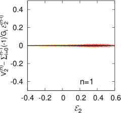
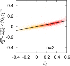
Fig. 1: Linear relations respectively from the real part (red points) and the imaginary part (yellow points) for $n=1$ and $n=2$, from hydro simulations with constant $\eta/s=0.08$. Slopes of solid lines are determined from the values of $G_{1}$ and $G_{2}$ respectively.

Fig. 2 shows the numerical results of about 1000 events from hydrodynamic simulations with different values of $\eta/s$ from 0.001 to 0.2. The obtained length of the two-point correlation of $V_{2}$ defined in Eq. (7) is plotted as a function of $\eta/s$, which agrees with the expectation from Eq. (8) within statistical errors. This indicates that the increase of the two-point correlation length in elliptic flow comparing to that in the initial eccentricity is purely an effect of fluid dynamics. One can also see that the two-point correlation at the final stage is reduced as the increase of $\eta/s$. This can be understood as a direct consequence of sound propagation, reflected in the ratio $G_{2}/G_{0}$ [11]. Since sound propagation is damped as a result of fluid dissipation, the two-point correlation at the final stage is reduced.

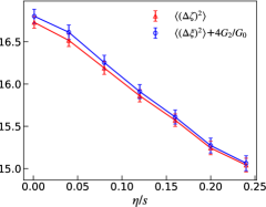
Fig. 2: Two-point correlation length of $V_{2}$ and the expectations from Eq. (8), as a function of $\eta/s$, where the initial two-point correlation length is $\left\langle(\Delta\xi)^{2}\right\rangle=12.81\pm 0.08$. Figure taken from Ref. [5].

In summary, we have derived the differential formulation of pseudorapidity dependent hydrodynamic response which is different from some previous studies (cf. [12, 13]). The formulation is expected to be applicable to other flow harmonics as well, when nonlinear response is not dominant in flow generation [4, 14]. Through the event-by-event simulations of 3+1D MUSIC, with initial conditions generated via the AMPT model, the differential response relation is verified. We also find that the increase of the two-point correlation of elliptic flow comparing to that in the initial eccentricity is purely an effect of fluid dynamics.

4 Acknowledgements

This work is supported by National Natural Science Foundation of China (NSFC) under Grant No. 11975079 (LY) and China Postdoctoral Science Foundation under Grant No. 2019M661333 (HL).

References

- [1] J.-Y. Ollitrault, Anisotropy as a signature of transverse collective flow, Phys. Rev. D46 (1992) 229–245. doi:10.1103/PhysRevD.46.229.
- [2] Z. Qiu, U. W. Heinz, Event-by-event shape and flow fluctuations of relativistic heavy-ion collision fireballs, Phys. Rev. C84 (2011) 024911. arXiv:1104.0650, doi:10.1103/PhysRevC.84.024911.
- [3] H. Niemi, G. S. Denicol, H. Holopainen, P. Huovinen, Event-by-event distributions of azimuthal asymmetries in ultrarelativistic heavy-ion collisions, Phys. Rev. C87 (5) (2013) 054901. arXiv:1212.1008, doi:10.1103/PhysRevC.87.054901.
- [4] J. Noronha-Hostler, L. Yan, F. G. Gardim, J.-Y. Ollitrault, Linear and cubic response to the initial eccentricity in heavy-ion collisions, Phys. Rev. C93 (1) (2016) 014909. arXiv:1511.03896, doi:10.1103/PhysRevC.93.014909.
- [5] H. Li, L. Yan, Pseudorapidity dependent hydrodynamic response in heavy-ion collisionsarXiv:1907.10854, doi:10.1016/j.physletb.2020.135248.
- [6] R. Franco, M. Luzum, Rapidity-dependent eccentricity scaling in relativistic heavy-ion collisionsarXiv:1910.14598.
- [7] B. Schenke, S. Jeon, C. Gale, (3+1)D hydrodynamic simulation of relativistic heavy-ion collisions, Phys. Rev. C82 (2010) 014903. arXiv:1004.1408, doi:10.1103/PhysRevC.82.014903.
- [8] B. Schenke, S. Jeon, C. Gale, Elliptic and triangular flow in event-by-event (3+1)D viscous hydrodynamics, Phys. Rev. Lett. 106 (2011) 042301. arXiv:1009.3244, doi:10.1103/PhysRevLett.106.042301.
- [9] Z.-W. Lin, C. M. Ko, B.-A. Li, B. Zhang, S. Pal, A Multi-phase transport model for relativistic heavy ion collisions, Phys. Rev. C72 (2005) 064901. arXiv:nucl-th/0411110, doi:10.1103/PhysRevC.72.064901.
- [10] H. Li, L.-G. Pang, Q. Wang, X.-L. Xia, Global polarization in heavy-ion collisions from a transport model, Phys. Rev. C96 (5) (2017) 054908. arXiv:1704.01507, doi:10.1103/PhysRevC.96.054908.
- [11] J. I. Kapusta, B. Muller, M. Stephanov, Relativistic Theory of Hydrodynamic Fluctuations with Applications to Heavy Ion Collisions, Phys. Rev. C85 (2012) 054906. arXiv:1112.6405, doi:10.1103/PhysRevC.85.054906.
- [12] P. Bozek, W. Broniowski, A. Olszewski, Hydrodynamic modeling of pseudorapidity flow correlations in relativistic heavy-ion collisions and the torque effect, Phys. Rev. C91 (2015) 054912. arXiv:1503.07425, doi:10.1103/PhysRevC.91.054912.
- [13] A. Sakai, K. Murase, T. Hirano, Rapidity decorrelation from hydrodynamic fluctuations, Nucl. Phys. A982 (2019) 339–342. arXiv:1807.06254, doi:10.1016/j.nuclphysa.2018.08.012.
- [14] D. Teaney, L. Yan, Non linearities in the harmonic spectrum of heavy ion collisions with ideal and viscous hydrodynamics, Phys. Rev. C86 (2012) 044908. arXiv:1206.1905, doi:10.1103/PhysRevC.86.044908.