Abstract

For a high-dimensional linear model with a finite number of covariates measured with error, we study statistical inference on the parameters associated with the error-prone covariates, and propose a new corrected decorrelated score test and the corresponding one-step estimator. We further established asymptotic properties of the newly proposed test statistic and the one-step estimator. Under local alternatives, we show that the limiting distribution of our corrected decorrelated score test statistic is non-central normal. The finite-sample performance of the proposed inference procedure is examined through simulation studies. We further illustrate the proposed procedure via an empirical analysis of a real data example.

Keywords: Measurement error model, high-dimensional inference, decorrelated score function, nuisance parameter

1 Introduction

High dimensional data becomes more and more common in diverse fields such as computational biology, economics and climate science. Many statistical procedures have been developed for analysis of high dimensional data. However, most of them often assume that all covariates are measured accurately. In reality, measurement errors are ubiquitous in many high-dimensional problems, for example, measurements of gene expression with cDNA or oligonucleotide arrays (Rocke & Durbin, 2001) and sensor network data (Slijepcevic et al., 2002). This work was motivated by an empirical analysis of a real data set in Section 4.2, where both finite-dimensional phenotypic covariates and high-dimensional SNPs are available and one of the phenotypic covariates is of clinical interest but measured with error.

The classical measurement error models, where the number of covariates $p$ is fixed or is smaller than the sample size $n$, have been studied systematically, see Fuller (1987), Carroll et al. (2006), Yi (2016) and Ma & Li (2010). Penalized methods have been developed for high-dimensional linear measurement error models with $p>n$. Consider the model

$${\bf Y}={\bf X}{\boldsymbol{\theta}}_{0}+\boldsymbol{\epsilon},\ \ \text{and}\ \ {\bf W}={\bf X}+{\bf U},$$ (1)

where random vectors ${\bf Y},\boldsymbol{\epsilon}\in\mathbb{R}^{n}$, the $n\times p$ matrix ${\bf X}$ is unobservable, ${\bf W}$ is its observed surrogate, and the matrix ${\bf U}$ is random noise, i.e. measurement error. This is a difficult problem. In fact, even in the absence of measurement error, Zhao & Yu (2006) and Meinshausen et al. (2006) showed that the Lasso or Dantzig selector often fails in identifying significant covariates in high-dimensional models. With measurement error, Rosenbaum et al. (2010) showed that the true selection is likely to be outside of the feasible set of the Dantzig selector. Sørensen et al. (2015) analyzed the impact of measurement error on the standard Lasso and showed that treating ${\bf W}$ as the true ${\bf X}$ leads to erroneous results.

To correct the bias caused by the measurement error ${\bf U}$, a corrected objective function is

$$\frac{1}{2}{\boldsymbol{\theta}}^{\rm T}\widehat{\bf\Sigma}{\boldsymbol{\theta}}-\frac{1}{n}{\bf W}^{\rm T}{\bf y}+P_{\lambda}({\boldsymbol{\theta}}),$$

where $P_{\lambda}({\boldsymbol{\theta}})$ is a penalty with tuning parameter $\lambda$, $\widehat{\bf\Sigma}={\bf W}^{\rm T}{\bf W}/n-{\bf D}$, and ${\bf D}$ is the $p\times p$ covariance matrix of ${\bf U}_{i}$. Since $\widehat{\bf\Sigma}$ can have negative eigenvalues when $p$ is larger than $n$, the loss function ${\boldsymbol{\theta}}^{\rm T}\widehat{\bf\Sigma}{\boldsymbol{\theta}}/2-{\bf X}^{\rm T}{\bf y}/n$ is no longer convex. To overcome the difficulties caused by the non-convexity, Loh & Wainwright (2012) proposed a projected gradient descent algorithm that finds a possible local optimum with strong performance guarantees. Chen & Caramanis (2013) developed a simple variant of orthogonal matching pursuit algorithm that performs at the minimax optimal rate. Later, Belloni, Rosenbaum & Tsybakov (2017) proposed the compensated matrix uncertainty (MU) selector, which can be written as a second-order cone programming minimization problem and the estimator attains the minimax efficiency bound. Loh et al. (2017) developed a primal-dual witness proof framework to establish the estimator error bounds in different norms in general sparse regression problems with non-convex loss function and penalty. This work does not require the typical incoherence condition, but need to impose the constraint $\|{\boldsymbol{\theta}}_{0}\|_{1}<R$. Datta et al. (2017) proposed CoCoLasso estimator which forces the non-convex problem to be convex by applying a nearest positive semi-definite matrix projection operator to $\widehat{\bf\Sigma}$, which can be solved by the ADMM algorithm, and analyzed its error bounds with deterministic design matrix ${\bf X}$. Under a slightly stronger sparsity conditions, the asymptotic sign-consistency properties were established.

The aforementioned works focus on the theory and numerical algorithms of regularization methods rather than statistical inference. It is important to quantify the uncertainty of an estimator in high dimensional linear measurement error models. Recently, significant progress has been made regarding hypothesis testing on low dimensional sub-parameters in high dimensional sparse models. From a semiparametric perspective, the challenges in these problems lie in how to handle the effect of high-dimensional nuisance parameters and correct the bias of the estimators for the low dimensional parameters of interest caused by the penalty. Zhang & Zhang (2014) proposed a low dimensional projection (LDP) approach to construct bias-corrected linear Lasso estimator and corresponding confidence intervals without assuming the uniform signal strength condition (Wainwright, 2009). Van de Geer et al. (2014) exploited the idea of inverting the Karush-Kuhn-Tucker characterization to desparsify Lasso, which essentially leads to the same results as in Zhang & Zhang (2014) for a linear model. Javanmard & Montanari (2014) proposed to debias the Lasso estimator by adding a term proportional to the subgradient of the $\ell_{1}$ norm at the Lasso solution, and the confidence intervals constructed based on the debiased estimator have nearly optimal size. All these works assume either linear or generalized linear models. Ning et al. (2017) provided a general framework for high-dimensional inference by proposing a decorrelated score function. By applying a decorrelation operation on the high-dimensional score functions, the derived decorrelated score function is uncorrelated with the nuisance score function. In this case, the efficiency of the estimators for the parameters of interest will not be impaired provided that the estimators for the nuisance parameters are consistent at sufficient rate.

Inference for high dimensional measurement error models is believed to be a difficult topic due to the bias and lack of power introduced by measurement error as well as high dimensional nuisance parameters. Recently, Belloni, Chernozhukov & Kaul (2017) constructed simultaneous confidence regions for the parameters of interest in high-dimensional linear models with error-in-variables using multiplier bootstrap. Wang et al. (2019) employed a de-biasing approach and constructed component-wise confidence intervals in a sparse high-dimensional linear regression model when some covariates of the design matrix are missing completely at random. In this paper, we consider the setting where only a fixed number of covariates are measured with error and our goal is to develop statistical inference procedures for the coefficients of these covariates. In practice, it is common that not all covariates are corrupted. For example, in the real data example analyzed in Section 4.2, covariates such as gender and age are measured precisely. Moreover, it is in general very difficult to find a good estimate for the $p\times p$ covariance matrix ${\bf D}$ of measurement error without any strong and restrictive assumptions.

We extend the inference results of low dimensional linear measurement error models to high dimensional settings, which is important yet challenging, and requires vastly different treatments. In the spirit of semiparametrics, we employ decorrelation operation to control the impact of high-dimensional nuisance parameters, and construct a corrected decorrelated score function for the parameters of interest. The performance of the corrected decorrelated score test relies on the convergence rate of the initial estimator. The asymptotic normality of the corrected decorrelated score test statistic holds provided that the initial estimator is statistically consistent at certain rate. Here, we take the CoCoLasso estimator (Datta et al., 2017) as an example. Indeed, any estimator with sufficient convergence rate can be served as the initial estimator in forming the decorrelated score function. Different from the settings in Datta et al. (2017), we assume that the design is random and sub-Gaussian, and only a fixed number of covariates, without loss of generality, one covariate, is measured with error. We rederive the theoretical properties of the CoCoLasso estimator in our new settings, which is one of the contributions of this work. Our corrected decorrelated score test statistics retain power under the local alternatives around $0$, because we essentially do not impose any penalty on the parameter of interest in the construction. We further construct confidence intervals by proving the limiting distribution of the one-step estimator, which is semiparametrically efficient. Note that although we write our development for one variable with measurement error, the proposed method is directly applicable to a finite number of covariates with measurement error naturally.

Our work extends the key idea of semiparametrics to inference in high dimensional linear measurement error models. We handle the sparsity assumptions differently from Belloni, Rosenbaum & Tsybakov (2017) and Loh & Wainwright (2012), and extend the results in Datta et al. (2017) to random sub-Gaussian designs. Although a general framework of inference was provided in Ning et al. (2017), the existence of measurement errors imposes many special challenges in methodology and theoretical proofs, which requires innovative technical treatments, as illustrated in the main text of the paper. Compared to Belloni, Chernozhukov & Kaul (2017), we avoid solving estimating equations completely. Our one-step estimator has the same limiting distribution as that of the root of estimating equations but is much easier to compute.

We specify the model for high-dimensional data with one covariate with measurement error and develop the methodology in Section 2, which includes construction of the corrected decorrelated score function, statistical properties of the initial estimator as well as the algorithm. Technical conditions, asymptotic properties of the score test statistic and the one-step estimator are established in Section 3. To assess the performance of our method, we conduct simulation studies and perform an empirical data analysis in Section 4.

Notations and Preliminaries: Before we pursue further, let us introduce some notation and some preliminaries. For a vector ${\bf v}=(v_{1},\dots,v_{p})^{\rm T}\in\mathbb{R}^{p}$, we define $\|{\bf v}\|_{0}=|\rm{supp}({\bf v})|$, where $\rm{supp}({\bf v})=\{j:v_{j}\neq 0\}$ and $|A|$ is the cardinality of a set $A$. Denote $\|{\bf v}\|_{\infty}=\max_{1\leq j\leq p}|v_{j}|$ and ${\bf v}^{\otimes 2}={\bf v}{\bf v}^{\rm T}$. For $S\subseteq\{1,\dots,p\}$, let ${\bf v}_{S}=\{v_{j}:j\in S\}$ and $S^{C}$ be the complement of $S$ . For a matrix ${\bf M}=[{\bf M}_{jk}]$, let $\|{\bf M}\|_{\max}=\max_{j,k}|M_{jk}|$, $\|M\|_{\infty}=\max_{j}\sum_{k}|M_{jk}|$ and ${\bf M}^{\otimes 2}={\bf M}{\bf M}^{\rm T}$. If ${\bf M}$ is symmetric, then $\lambda_{\min}({\bf M})$ and $\lambda_{\max}({\bf M})$ are the minimal and maximal eigenvalues of ${\bf M}$. For two positive sequences $a_{n}$ and $b_{n}$, we use $a_{n}\precsim b_{n}$ to denote $a_{n}\leq Cb_{n}$ for some constant $C>0$, and use $a_{n}\asymp b_{n}$ to denote $C\leq a_{n}/b_{n}\leq C^{\prime}$ for some constants $C,C^{\prime}>0$. Denote $\Phi(\cdot)$ to be the cumulative distribution function of the standard normal distribution. For simplicity, we use $E(\cdot)$ and $\Pr(\cdot)$ to denote the expectation and probability calculated under the true model, respectively.

The sub-exponential norm of a random variable $X$ is defined as $\|X\|_{\psi_{1}}=\sup_{q\geq 1}q^{-1}\{E(|X|^{q})\}^{1/q}$. Note that $\|X\|_{\psi_{1}}<C_{1}$ for some constant $C_{1}$, if $X$ is sub-exponential. The sub-Gaussian norm of $X$ is defined as $\|X\|_{\psi_{2}}=\sup_{q\geq 1}q^{-1/2}\{E(|X|^{q})\}^{1/q}$. Note that $\|X\|_{\psi_{2}}<C_{2}$ for some constant $C_{2}$, if $X$ is sub-Gaussian. More properties regarding sub-exponential and sub-Gaussian random variables are given in Appendix G.1 in the supplementary materials.

2 Model Setup and Proposed Method

2.1 Model Specification

Suppose that $\{Y_{i},W_{i},{\bf Z}_{i}\}$, $i=1,\dots,n$, is an independent and identically distributed sample from a linear model with one of the covariates measured with additive error

$$Y_{i}=\beta_{0}X_{i}+{\boldsymbol{\gamma}}_{0}^{\rm T}{\bf Z}_{i}+\epsilon_{i}\ \ \text{and}\ \ W_{i}=X_{i}+U_{i}.$$ (2)

Covariate $X_{i}\in\mathbb{R}$ is unobservable, and $W_{i}$ is its error-prone surrogate. Covariate vector ${\bf Z}_{i}\in\mathbb{R}^{p-1}$ is measured precisely. Assume that $(X_{i},{\bf Z}_{i}^{\rm T})^{\rm T}$ is sub-Gaussian element-wise with mean ${\bf 0}$ and unit diagonal covariance matrix. To exclude the intercept term in the model, we let the response $Y_{i}$ have mean 0 as well. The regression error $\epsilon_{i}$ is sub-Gaussian with mean 0, variance $\sigma_{\epsilon}^{2}$, and sub-Gaussian norm $K_{\epsilon}$. The measurement error $U_{i}$ is also sub-Gaussian with mean 0, variance $\sigma_{U}^{2}$, and sub-Gaussian norm $K_{U}$. It is independent of $\epsilon_{i}$, $X_{i}$ and ${\bf Z}_{i}$. As in the literature, we assume that $\sigma_{U}^{2}$ and $E(U_{i}^{4})$ are known.

Let ${\bf Y}=(Y_{1},\dots,Y_{n})^{\rm T}$, ${\bf X}=(X_{1},\dots,X_{n})^{\rm T}$, ${\bf W}=(W_{1},\dots,W_{n})^{\rm T}$ and ${\bf Z}=({\bf Z}_{1},\dots,{\bf Z}_{n})^{\rm T}$ denote the corresponding vector or matrix version of $n$ samples. In practice, we only need to center all variables, and standardize the columns of the data matrix such that $\sum_{i=1}^{n}Z_{ij}^{2}/n=1$ and $\sum_{i=1}^{n}W_{i}^{2}/n=1+\sigma_{U}^{2}$ for $j=1,\dots,p-1$ and $i=1,\dots,n$ .

For the purpose of theoretical proofs, we have the following standard assumptions.

Assumption 1.

Assume that

• $2\kappa\leq\lambda_{\min}[E\{(X_{i},{\bf Z}_{i}^{\rm T})^{{}^{\rm T}\otimes 2}\}]\leq\lambda_{\max}[E\{(X_{i},{\bf Z}_{i}^{\rm T})^{{}^{\rm T}\otimes 2}\}]\leq 2/\kappa$ for some constant $\kappa>0$;

• $\|Z_{ij}\|_{\psi_{2}}$ and $\|X_{i}\|_{\psi_{2}}$ are uniformly bounded by some constant $K$ for $j=1,\dots,p-1$;

• The true parameter ${\boldsymbol{\theta}}_{0}=(\beta_{0},{\boldsymbol{\gamma}}_{0}^{\rm T})^{\rm T}$ is sparse with support $S$, and $|S|=s_{0}$; Let $\|{\boldsymbol{\theta}}_{0}\|_{\infty}\leq K_{0}$, where $K_{0}$ is a positive constant;

• $E(X_{i}{\bf Z}_{i}^{\rm T})\{E({\bf Z}_{i}^{\otimes 2})\}^{-1}$ is sparse with support $S^{\prime}$ and $|S^{\prime}|=s^{\prime}$. Moreover,

  $\|E(X_{i}{\bf Z}_{i}^{\rm T})\{E({\bf Z}_{i}^{\otimes 2})\}^{-1}\|_{1}\leq K_{\boldsymbol{\omega}}$ for some constant $K_{\boldsymbol{\omega}}>0$.

In Assumption 1, ${\rm(i)}$ and ${\rm(ii)}$ are common assumptions for high dimensional random designs. Assumption ${\rm(iii)}$ is about the sparsity of the true model (2). Instead of assuming $\|{\boldsymbol{\theta}}_{0}\|_{1}$ is bounded, we only assume the $l_{\infty}$ norm of ${\boldsymbol{\theta}}_{0}$ is bounded. Assumption ${\rm(iv)}$ is crucial in the inference framework of Ning et al. (2017). When conducting decorrelation operation, their key assumption is that the projection of the score function for $\beta$ to the linear space spanned by the nuisance score functions for ${\boldsymbol{\gamma}}$, denoted as $\Lambda_{{\boldsymbol{\gamma}}}$, is identical to the projection of the score function for $\beta$ to a low dimensional subspace of $\Lambda_{{\boldsymbol{\gamma}}}$. More details about the motivation of sparse projection and the formation of $E(X_{i}{\bf Z}_{i}^{\rm T})\{E({\bf Z}_{i}^{\otimes 2})\}^{-1}$ will be discussed in Section 2.2.

Our goal is to test the hypothesis $H_{0}:\beta_{0}=\beta^{*}$ and construct valid confidence intervals for $\beta_{0}$ when the dimension of ${\boldsymbol{\theta}}_{0}=(\beta_{0},{\boldsymbol{\gamma}}_{0}^{\rm T})^{\rm T}$ is much larger than the sample size $n$, that is, $p\gg n$. Note that when $\beta^{*}=0$, under the null hypothesis, the model degenerates to a linear model without measurement error, hence testing procedures for high dimensional sparse linear models can be applied. In this paper, we consider a general hypothesis test setting where $\beta^{*}\in\mathbb{R}$.

2.2 Corrected Decorrelated Score Function

If covariate $X$ is observed with no measurement error, it is known that the loss function based on least squares is ${\boldsymbol{\theta}}^{\rm T}{\bf\Sigma}{\boldsymbol{\theta}}/2-{\boldsymbol{\rho}}^{\rm T}{\boldsymbol{\theta}}$, where ${\bf\Sigma}=({\bf X},{\bf Z})^{\rm T}({\bf X},{\bf Z})/n$ and ${\boldsymbol{\rho}}=({\bf X},{\bf Z})^{\rm T}{\bf Y}/n$. For our corrupted data $({\bf Y},{\bf W},{\bf Z})$, as emphasized above, instead of treating ${\bf W}$ as ${\bf X}$ in the loss function directly, we define the corrected loss function as

$$l({\boldsymbol{\theta}})=\frac{1}{2}{\boldsymbol{\theta}}^{\rm T}\widehat{\bf\Sigma}{\boldsymbol{\theta}}-\widehat{\boldsymbol{\rho}}^{\rm T}{\boldsymbol{\theta}},$$ (3)

where

$$\widehat{\bf\Sigma}=\frac{1}{n}({\bf W},{\bf Z})^{\rm T}({\bf W},{\bf Z})-\begin{pmatrix}\sigma_{U}^{2}&{\bf 0}\\ {\bf 0}&{\bf 0}\end{pmatrix}\ \ \text{and}\ \ \widehat{\boldsymbol{\rho}} = \frac{1}{n}({\bf W},{\bf Z})^{\rm T}{\bf Y}.$$

By assumption, $U_{i}$ is independent of $X_{i}$, ${\bf Z}_{i}$ and $\epsilon_{i}$, it is easy to verify that $E(\widehat{\bf\Sigma})=E({\bf\Sigma})$ and $E(\widehat{\boldsymbol{\rho}})=E({\boldsymbol{\rho}})$.

The gradient of the loss function plays an important role in statistical analysis. Because our corrected loss function is no longer the log-likelihood, we name it the gradient corrected score function, which has the form ${\bf S}_{{\boldsymbol{\theta}}}({\boldsymbol{\theta}})=n^{-1}\sum_{i=1}^{n}{\bf S}_{i{\boldsymbol{\theta}}}({\boldsymbol{\theta}})=\widehat{\bf\Sigma}{\boldsymbol{\theta}}-\widehat{\boldsymbol{\rho}}$. Because we aim at conducting inference on the parameter $\beta$, we treat the $p-1$ dimensional parameter ${\boldsymbol{\gamma}}$ as nuisance. Then the corrected score function can be decomposed as

$${\bf S}_{{\boldsymbol{\theta}}}({\boldsymbol{\theta}})=\begin{pmatrix}S_{\beta}(\beta,{\boldsymbol{\gamma}})\\ {\bf S}_{{\boldsymbol{\gamma}}}(\beta,{\boldsymbol{\gamma}})\end{pmatrix}=\begin{pmatrix}\widehat{\Sigma}_{11}\beta+\widehat{\bf\Sigma}_{12}{\boldsymbol{\gamma}}-\widehat{\rho}_{1}\\ \widehat{\bf\Sigma}_{21}\beta+\widehat{\bf\Sigma}_{22}{\boldsymbol{\gamma}}-\widehat{\boldsymbol{\rho}}_{2}\end{pmatrix},$$

where $\widehat{\Sigma}_{11}={\bf W}^{\rm T}{\bf W}/n-\sigma^{2}_{U}$, $\widehat{\bf\Sigma}_{12}={\bf W}^{\rm T}{\bf Z}/n$, $\widehat{\bf\Sigma}_{21}={\bf Z}^{\rm T}{\bf W}/n$, $\widehat{\bf\Sigma}_{22}={\bf Z}^{\rm T}{\bf Z}/n$, $\widehat{\rho}_{1}={\bf W}^{\rm T}{\bf Y}/n$ and $\widehat{\boldsymbol{\rho}}_{2}={\bf Z}^{\rm T}{\bf Y}/n$.

Similar to the standard score function, it can be easily verified that $E\{{\bf S}_{i{\boldsymbol{\theta}}}({\boldsymbol{\theta}}_{0})\}={\bf 0}$. Define the $p\times p$ corrected score covariance matrix as

$${\bf I}({\boldsymbol{\theta}})=E\{{\bf S}_{i{\boldsymbol{\theta}}}({\boldsymbol{\theta}}){\bf S}_{i{\boldsymbol{\theta}}}({\boldsymbol{\theta}})^{\rm T}\}=\begin{pmatrix}I_{\beta\beta}&{\bf I}_{\beta{\boldsymbol{\gamma}}}\\ {\bf I}_{{\boldsymbol{\gamma}}\beta}&{\bf I}_{{\boldsymbol{\gamma}}{\boldsymbol{\gamma}}}\end{pmatrix}.$$

Note that the covariance matrix ${\bf I}({\boldsymbol{\theta}})$ is no longer equal to $E\{\partial{\bf S}_{i{\boldsymbol{\theta}}}({\boldsymbol{\theta}})/\partial{\boldsymbol{\theta}}^{\rm T}\}$ due to the bias correction procedure in constructing the loss function. In fact, the matrix ${\bf I}({\boldsymbol{\theta}})$ has more complex form. With standardized data matrix $({\bf X},{\bf Z})$, by simple calculations we obtain that

$${\bf I}({\boldsymbol{\theta}})=\begin{pmatrix}(\sigma_{\epsilon}^{2}+\beta^{2}\sigma_{U}^{2})+\sigma_{\epsilon}^{2}\sigma_{U}^{2}+\beta^{2}E(U_{i}^{4})-\beta^{2}\sigma_{U}^{4}&(\sigma_{\epsilon}^{2}+\beta^{2}\sigma_{U}^{2})E(X_{i}{\bf Z}_{i})^{\rm T}\\ (\sigma_{\epsilon}^{2}+\beta^{2}\sigma_{U}^{2})E(X_{i}{\bf Z}_{i})&(\sigma_{\epsilon}^{2}+\beta^{2}\sigma_{U}^{2})E({\bf Z}_{i}{\bf Z}_{i}^{\rm T})\end{pmatrix}.$$ (4)

To control the impact of high-dimensional nuisance parameter ${\boldsymbol{\gamma}}$ on the inference of the parameter of interest $\beta$, we define the corrected decorrelated score function for $\beta$ as

$$S(\beta,{\boldsymbol{\gamma}})=S_{\beta}(\beta,{\boldsymbol{\gamma}})-\boldsymbol{\omega}^{\rm T}{\bf S}_{{\boldsymbol{\gamma}}}(\beta,{\boldsymbol{\gamma}}),$$

where $\boldsymbol{\omega}^{\rm T}={\bf I}_{\beta{\boldsymbol{\gamma}}}{\bf I}_{{\boldsymbol{\gamma}}{\boldsymbol{\gamma}}}^{-1}=E(X_{i}{\bf Z}_{i}^{\rm T})E({\bf Z}_{i}{\bf Z}_{i}^{\rm T})^{-1}=E(W_{i}{\bf Z}_{i}^{\rm T})E({\bf Z}_{i}{\bf Z}_{i}^{\rm T})^{-1}$. Under the assumption that the minimal eigenvalue of $E\{(X_{i},{\bf Z}_{i}^{\rm T})^{{}^{\rm T}\otimes{2}}\}$ is bounded and bounded away from $0$, it is easy to show that the $(p-1)\times(p-1)$ matrix $E({\bf Z}_{i}{\bf Z}_{i}^{\rm T})$ is invertible. Note that this construction ensures that $S(\beta,{\boldsymbol{\gamma}})$ is uncorrelated with the nuisance score function ${\bf S}_{{\boldsymbol{\gamma}}}(\beta,{\boldsymbol{\gamma}})$, i.e. $E\{S(\beta_{0},{\boldsymbol{\gamma}}_{0}){\bf S}_{{\boldsymbol{\gamma}}}(\beta_{0},{\boldsymbol{\gamma}}_{0})\}={\bf 0}$. The detailed verification is in Appendix D.1 in supplementary materials. We denote the variance of $S(\beta,{\boldsymbol{\gamma}})$ as $\sigma_{\beta\mid{\boldsymbol{\gamma}}}^{2}$, and it is easy to show that

$$\sigma^{2}_{\beta|{\boldsymbol{\gamma}}}=I_{\beta\beta}-{\bf I}_{\beta{\boldsymbol{\gamma}}}{\bf I}_{{\boldsymbol{\gamma}}{\boldsymbol{\gamma}}}^{-1}{\bf I}_{{\boldsymbol{\gamma}}\beta}.$$ (5)

Under the null hypothesis $H_{0}:\beta_{0}=\beta^{*}$, to construct score test statistic, we need to find estimators for the nuisance parameter ${\boldsymbol{\gamma}}$ and the $p-1$ dimensional vector $\boldsymbol{\omega}$. For ${\boldsymbol{\gamma}}$, we can use any consistent estimator $\widetilde{\boldsymbol{\gamma}}$ with sufficient convergence rate due to the decorrelation operation. More details about $\widetilde{\boldsymbol{\gamma}}$ as well as the initial estimator $\widetilde{\beta}$ for $\beta$ will be discussed in Section 2.3. For $\boldsymbol{\omega}$, an intuitive estimator is its sample version $\widehat{\bf\Sigma}_{12}\widehat{\bf\Sigma}_{22}^{-1}$. However, matrix $\widehat{\bf\Sigma}_{22}$ is not invertible when $p-1>n$. Ning et al. (2017) imposed sparsity assumption on $\boldsymbol{\omega}$ to control the estimation error. Many different penalized methods can be applied to obtain a sparse estimator of $\boldsymbol{\omega}$. For example, the Dantzig type estimator $\widehat{\boldsymbol{\omega}}$ can be obtained as follows:

$$\widehat{\boldsymbol{\omega}}=\operatorname*{arg\,min}\|\boldsymbol{\omega}\|_{1}\ \ \text{s.t.}\ \ \|\widehat{\bf\Sigma}_{12}-\boldsymbol{\omega}^{\rm T}\widehat{\bf\Sigma}_{22}\|_{\infty}\leq\lambda^{\prime},$$ (6)

where $\lambda^{\prime}$ is a tuning parameter. Note that in our model $\widehat{\bf\Sigma}_{12}$ and $\widehat{\bf\Sigma}_{22}$ do not depend on ${\boldsymbol{\theta}}$. Then the estimated corrected decorrelated score function is defined as $\widehat{S}(\beta,\widetilde{\boldsymbol{\gamma}})=S_{\beta}(\beta,\widetilde{\boldsymbol{\gamma}})-\widehat{\boldsymbol{\omega}}^{\rm T}{\bf S}_{{\boldsymbol{\gamma}}}(\beta,\widetilde{\boldsymbol{\gamma}})$.

Under the null hypothesis, we construct the test statistic as $\widehat{T}_{n}=n^{1/2}\widehat{S}(\beta^{*},\widetilde{\boldsymbol{\gamma}})(\widehat{\sigma}^{2}_{\beta|{\boldsymbol{\gamma}},H_{0}})^{-1/2}$, where

$$\widehat{\sigma}^{2}_{\beta|{\boldsymbol{\gamma}},H_{0}} = \{\widehat{I}_{\beta\beta}-\widehat{\boldsymbol{\omega}}^{\rm T}\widehat{\bf I}_{{\boldsymbol{\gamma}}\beta}\}|_{\beta=\beta^{*}}$$ (7)

$$= (\widehat{\sigma}_{\epsilon,H_{0}}^{2}+\beta^{*2}\sigma_{U}^{2})(1-\widehat{\boldsymbol{\omega}}^{\rm T}\widehat{\bf\Sigma}_{21})+\beta^{*2}E(U_{i}^{4})+\widehat{\sigma}_{\epsilon,H_{0}}^{2}\sigma_{U}^{2}-\beta^{*2}\sigma_{U}^{4},$$

and $\widehat{\sigma}_{\epsilon,H_{0}}^{2}=n^{-1}\sum_{i=1}^{n}(Y_{i}-\beta^{*}W_{i}-\widetilde{\boldsymbol{\gamma}}^{\rm T}{\bf Z}_{i})^{2}-\beta^{*2}\sigma_{U}^{2}$. The detailed derivation is given in Appendix D.2 in supplementary materials. Under some assumptions we will specify in Section 4, the test statistic $\widehat{T}_{n}$ is asymptotically standard normal, see Corollary 1.

For confidence interval construction, define the one-step estimator for $\beta$ as the root of the first order approximation of the approximately unbiased estimating equation $\widehat{S}(\beta,\widetilde{\boldsymbol{\gamma}})=0$ around the initial estimator $\widetilde{\beta}$, i.e.,

$$\widehat{\beta} = \widetilde{\beta}-\widehat{S}(\widetilde{\boldsymbol{\theta}})/\{\partial\widehat{S}(\beta,\widetilde{\boldsymbol{\gamma}})/\partial\beta\}|_{\beta=\widetilde{\beta}}$$

$$= \widetilde{\beta}-\widehat{S}(\widetilde{\boldsymbol{\theta}})/(\widehat{\bf\Sigma}_{11}-\widehat{\boldsymbol{\omega}}^{\rm T}\widehat{\bf\Sigma}_{21}).$$

Of course, we could use the true root of $\widehat{S}(\beta,\widetilde{\boldsymbol{\gamma}})=0$ as $\widehat{\boldsymbol{\beta}}$. Here, we choose to use the one-step update for its computational simplicity. In fact, we have proved that the asymptotic distribution of the one-step estimator is identical to that of the true root because we have a relatively good initial estimator $\widetilde{\boldsymbol{\beta}}$. We will show that the one-step estimator $\widehat{\beta}$ is consistent and asymptotically normal with asymptotic variance $\sigma_{\beta}^{2}$ under suitable assumptions in Theorem 2. Hence, the $(1-\alpha)100\%$ confidence interval for $\beta_{0}$ can be constructed as $\left(\widehat{\beta}-z_{\alpha}\sqrt{\widehat{\sigma}_{\beta}^{2}/n},\widehat{\beta}+z_{\alpha}\sqrt{\widehat{\sigma}_{\beta}^{2}/n}\right)$, where $\Phi(z_{\alpha})=1-\alpha/2$, and $\widehat{\sigma}_{\beta}^{2}$ is an estimate of $\sigma_{\beta}^{2}$ whose specific form is given in Theorem 2.

2.3 Initial Estimator

In the literature, estimation theories under different assumptions have been developed for model (1), where all covariates are measured with error, see Loh & Wainwright (2012), Chen & Caramanis (2013), Belloni, Rosenbaum & Tsybakov (2017), Loh et al. (2017) and Datta et al. (2017). With slight modifications, these methods can all be applied to our model to construct desired initial estimators. Here, we take CoCoLasso estimator proposed by Datta et al. (2017) as an example to show how the convergence performance of the initial estimator affects the inferential results of $\beta$.

The CoCoLasso estimator is defined as

$$\widetilde{\boldsymbol{\theta}}=\operatorname*{arg\,min}_{{\boldsymbol{\theta}}}\frac{1}{2}{\boldsymbol{\theta}}^{\rm T}\widetilde{\bf\Sigma}{\boldsymbol{\theta}}-\widehat{\boldsymbol{\rho}}^{\rm T}{\boldsymbol{\theta}}+\lambda\|{\boldsymbol{\theta}}\|_{1},$$ (8)

where $\widetilde{\bf\Sigma}=(\widehat{\bf\Sigma})_{+}$ and $\lambda$ is a tuning parameter. The nearest positive semi-definite matrix projection operator $(\cdot)_{+}$ is defined as follows: for any matrix ${\bf K}$,

$$({\bf K})_{+}=\operatorname*{arg\,min}_{{\bf K}_{1}\geq{\bf 0}}\|{\bf K}-{\bf K}_{1}\|_{\rm{max}}.$$

The ADMM algorithm is used to find the nearest positive semi-definite matrix. For more details, see Fan et al. (2016) and Datta et al. (2017).

As mentioned in the introduction, since we consider sub-Gaussian design with fixed number of covariates measured with error, which is different from the settings in Datta et al. (2017), we modified their theoretical proofs under our settings and the error bounds are different in terms of certain constants. We give the $l_{1}$, $l_{2}$ and prediction error bounds of $\widetilde{\boldsymbol{\theta}}$ in the following Lemma.

Lemma 1.

Let $\lambda=C_{\lambda}s_{0}\sqrt{n^{-1}{\rm log}p}=o(1)$. For $C_{\lambda}>\max\left(8K_{0}K_{2}/C^{\prime\prime},8\sqrt{2}K_{0}K_{3}/\sqrt{C^{\prime\prime}}\right)$ and $\lambda\leq\min(8K_{1},16KK_{\epsilon},8K_{0}K_{2},8K_{0}K_{3})$, with probability at least $1-C_{1}\exp(-C_{2}{\rm log}p)$, we have

$$\|\widetilde{\boldsymbol{\theta}}-{\boldsymbol{\theta}}_{0}\|_{1}\leq 16\lambda s_{0}/\kappa,\ \ \|\widetilde{\boldsymbol{\theta}}-{\boldsymbol{\theta}}_{0}\|_{2}\leq\sqrt{32s_{0}}\lambda/\kappa,\ \ \text{and}\ \ \|({\bf X},{\bf Z})({\boldsymbol{\theta}}_{0}-\widetilde{\boldsymbol{\theta}})\|_{2}/\sqrt{n}\leq\lambda\sqrt{32s_{0}/\kappa},$$

where $\|{\boldsymbol{\theta}}_{0}\|_{\infty}\leq K_{0}$, $C^{\prime\prime}$ is a universal constant, $C_{1}$ and $C_{2}$ are positive constants depending on $K$, $K_{\epsilon}$, $K_{U}$, $K_{0}$, $\kappa$ and $\sigma_{U}^{2}$ given in the proof, $K_{1}=2K_{U}(K_{0}K+K_{\epsilon})$, $K_{2}=4K(K+K_{U})+2K_{U}^{2}+\sigma_{U}^{2}$ and $K_{3}=4(K+K_{U})^{2}+2\sigma_{U}^{2}$.

The detailed proof is given in Appendix E.1 in supplementary materials. It is based on the closeness condition for $\widehat{\bf\Sigma}$ and $\widehat{\boldsymbol{\rho}}$, and the restricted eigenvalue (RE) condition for matrix ${\bf\Sigma}$. Different from deterministic design, Bernstein inequalities were used repeatedly and we have shown that under the assumption that $s_{0}\sqrt{n^{-1}{\rm log}p}$ = o(1), the RE condition for sub-Gaussian matrix ${\bf\Sigma}$ holds with probability at least $1-2p^{-\zeta}$ in Lemma F.2 in supplementary materials.

For the $l_{\infty}$ error bound, for simplicity, slightly different notations are used here. Specifically, we write ${\boldsymbol{\theta}}_{0}=({\boldsymbol{\theta}}_{0,S}^{\rm T},{\bf 0}^{\rm T})^{\rm T}$, $({\bf X},{\bf Z})=({\bf Q}_{S},{\bf Q}_{S^{C}})$, and then partition the matrix ${\bf\Sigma}$ as

$${\bf\Sigma}=\begin{pmatrix}&n^{-1}{\bf Q}_{S}^{\rm T}{\bf Q}_{S}&n^{-1}{\bf Q}_{S}^{\rm T}{\bf Q}_{S^{C}}\\ &n^{-1}{\bf Q}_{S^{C}}^{\rm T}{\bf Q}_{S}&n^{-1}{\bf Q}_{S^{C}}^{\rm T}{\bf Q}_{S^{C}}\end{pmatrix}=\begin{pmatrix}{\bf\Sigma}_{S,S}&{\bf\Sigma}_{S,S^{C}}\\ {\bf\Sigma}_{S^{C},S}&{\bf\Sigma}_{S^{C},S^{C}}\end{pmatrix}.$$

To clarify, the above partition is based on the true support of model (2), that is, whether ${\bf X}$ is a part of ${\bf Q}_{S}$ depends on the true value $\beta_{0}$. Actually, when deriving the $l_{\infty}$ error bound for $\widetilde{\boldsymbol{\theta}}$, whether $\beta_{0}$ equals $0$ would not affect the proof as well as the theoretical result. To derive the $l_{\infty}$ error bound for $\widetilde{\boldsymbol{\theta}}$, we need to further assume that

$$\lambda_{\min}\{E({\bf\Sigma}_{S,S})\}=\kappa_{S}>0,\ \ \text{and}\ \ \|E({\bf\Sigma}_{S^{C},S})\{E({\bf\Sigma}_{S,S})\}^{-1}\|_{\infty}\leq 1-{\boldsymbol{\gamma}},$$ (9)

for some ${\boldsymbol{\gamma}}\in(0,1]$. Let $\|E({\bf\Sigma}_{S,S})^{-1}\|_{\infty}=\phi$ and $\|E({\bf\Sigma}_{S,S})^{-1}\|_{\infty}=\Phi$. The $l_{\infty}$ error bound result is stated as follows, which are similar to those given in Theorem 2 in Datta et al. (2017) with minor modifications. The detailed proof is given in the Appendix E.2 in the supplementary materials.

Lemma 2.

Let $\lambda=C_{\lambda}s_{0}\sqrt{n^{-1}{\rm log}p}=o(1)$. Under the assumptions given in (9) and $C_{\lambda}>8K_{4}/(\gamma\sqrt{C^{\prime\prime}})$, where $K_{4}=2K^{2}K_{0}+2KK_{\epsilon}$

1. With probability at least $1-p_{1}(\delta)$, there exists a unique solution $\widetilde{\boldsymbol{\theta}}$ minimizing ${\boldsymbol{\theta}}^{\rm T}\widetilde{\bf\Sigma}{\boldsymbol{\theta}}/2-\widehat{\boldsymbol{\rho}}^{\rm T}{\boldsymbol{\theta}}+\lambda\|{\boldsymbol{\theta}}\|_{1}$ whose support is a subset of the true support.

2. With probability at least $1-p_{2}(\delta^{\prime})$, $\|\widetilde{\boldsymbol{\theta}}_{S}-{\boldsymbol{\theta}}_{0S}\|_{\infty}\leq C_{\infty}\lambda$, where $C_{\infty}=8\phi$.

Probabilities $p_{1}(\delta)$ and $p_{2}(\delta^{\prime})$ go to zero as $n$ goes to infinity and the detailed expressions are given in Appendix E.2 in supplementary materials.

Note that Parts (a) and (b) of Lemma 2 imply that under the given conditions, $\|\widetilde{\boldsymbol{\theta}}-{\boldsymbol{\theta}}_{0}\|_{\infty}=\|\widetilde{\boldsymbol{\theta}}_{S}-{\boldsymbol{\theta}}_{0S}\|_{\infty}\leq C_{\infty}\lambda$ with probability at least $1-p_{1}(\delta)-p_{2}(\delta^{\prime})$.

Remark 1.

Note that we use $\widetilde{\bf\Sigma}$ in the loss function for CoCoLasso estimator to make the problem convex, but use $\widehat{\bf\Sigma}$ in the loss function to construct decorrelated score function. This discrepancy does not cause any problem when deriving the theoretical properties of our corrected score test statistic and one-step estimator.

Remark 2.

For CoCoLasso estimator, the tuning parameter $\lambda$ has the order $s_{0}\sqrt{n^{-1}{\rm log}p}$. However, in Loh et al. (2017), the tuning parameter has the order $\sqrt{n^{-1}{\rm log}p}$ under the assumption that $\|{\boldsymbol{\theta}}_{0}\|_{1}$ is bounded. In our proofs, we only assume that $\|{\boldsymbol{\theta}}_{0}\|_{\infty}$ is bounded. With the stronger assumption that $\|{\boldsymbol{\theta}}_{0}\|_{1}$ is bounded, the error bounds of CoCoLasso estimator would have the same order as those proposed in Loh et al. (2017) and Belloni, Rosenbaum & Tsybakov (2017).

2.4 Algorithm

Now we summarize the proposed estimation procedure as the following algorithm.

1. Calculate the initial CoCoLasso estimator $\widetilde{\boldsymbol{\theta}}=(\widetilde{\beta},\widetilde{\boldsymbol{\gamma}}^{\rm T})^{\rm T}$.

2. Estimate $\boldsymbol{\omega}$ by the Dantzig type estimator $\widehat{\boldsymbol{\omega}}$,

   $$\widehat{\boldsymbol{\omega}}=\operatorname*{arg\,min}\|\boldsymbol{\omega}\|_{1}\ \ \text{s.t.}\ \ \|\widehat{\bf\Sigma}_{12}-\boldsymbol{\omega}^{\rm T}\widehat{\bf\Sigma}_{22}\|_{\infty}\leq\lambda^{\prime},$$

   where $\lambda^{\prime}=O(\sqrt{{\rm log}p/n})$. For the detailed algorithm, see Candes et al. (2007). Note that other penalized M-estimators can also be used to solve for $\widehat{\boldsymbol{\omega}}$, for example, the Lasso.

3. Calculate the estimated decorrelated score function

   $$\widehat{S}(\beta,\widetilde{\boldsymbol{\gamma}})=S_{\beta}(\beta,\widetilde{\boldsymbol{\gamma}})-\widehat{\boldsymbol{\omega}}^{\rm T}{\bf S}_{{\boldsymbol{\gamma}}}(\beta,\widetilde{\boldsymbol{\gamma}}),$$

   and the test statistic $\widehat{T}_{n}=n^{1/2}\widehat{S}(\beta^{*},\widetilde{\boldsymbol{\gamma}})(\widehat{\sigma}^{2}_{\beta|{\boldsymbol{\gamma}},H_{0}})^{-1/2}$, where $\widehat{\sigma}^{2}_{\beta|{\boldsymbol{\gamma}},H_{0}}$ is given in (7). Under the conditions given in Theorem 1, the test statistic $\widehat{T}_{n}$ is asymptotically standard normal.

4. Calculate the one-step estimator

   $$\widehat{\beta} = \widetilde{\beta}-\widehat{S}(\widetilde{\boldsymbol{\theta}})/\{\partial\widehat{S}(\beta,\widetilde{\boldsymbol{\gamma}})/\partial\beta\}|_{\beta=\widetilde{\beta}}$$

   $$= \widetilde{\beta}-\widehat{S}(\widetilde{\boldsymbol{\theta}})/(\widehat{\bf\Sigma}_{11}-\widehat{\boldsymbol{\omega}}^{\rm T}\widehat{\bf\Sigma}_{21}).$$

   Construct the $(1-\alpha)100\%$ confidence interval for $\beta_{0}$ as $[\widehat{\beta}-z_{\alpha}\sqrt{\widehat{\sigma}_{\beta}^{2}/n},\widehat{\beta}+z_{\alpha}\sqrt{\widehat{\sigma}_{\beta}^{2}/n}]$, where $\Phi(z_{\alpha})=1-\alpha/2$, and $\widehat{\sigma}_{\beta}^{2}$ is given in Theorem 2.

3 Theory for Test and Confidence Intervals

We first establish four technical lemmas 3, 4, 5 and 6 to ensure the asymptotic normality of the corrected score test statistic $\widehat{T}_{n}$ and the one-step estimator $\widehat{\beta}$. Detailed descriptions of the four lemmas are given in Appendix A.

3.1 Corrected Score Test

Theorem 1.

Under conditions of Lemmas 3 - 5 and under $H_{0}:\beta_{0}=\beta^{*}$, it follows that

$$n^{1/2}\widehat{S}(\beta^{*},\widetilde{\boldsymbol{\gamma}})(\sigma^{2}_{\beta|{\boldsymbol{\gamma}},0})^{-1/2}\to N(0,1)$$

in distribution.

In Theorem 1, we state the asymptotic normality of the decorrelated score test statistic by assuming its true variance is known. The detailed proof is given in Appendix B.1. To show the asymptotic properties of the test statistic $\widehat{T}_{n}$ with estimated variance $\widehat{\sigma}^{2}_{\beta\mid{\boldsymbol{\gamma}},H_{0}}$, we need to further study the difference between $\widehat{\sigma}^{2}_{\beta\mid{\boldsymbol{\gamma}},H_{0}}$ and $\sigma^{2}_{\beta|{\boldsymbol{\gamma}},0}$, which is more complex than that of linear models without measurement error. We need to use $l_{\infty}$ error bound of $\widetilde{\boldsymbol{\gamma}}-{\boldsymbol{\gamma}}_{0}$ to facilitate the proof. Under a stronger assumption that $s_{0}^{3}\sqrt{n^{-1}{\rm log}p}=o(1),$ we show that $\widehat{T}_{n}$ is still asymptotically standard normal in the following corollary and detailed proof can be found in Appendix B.2.

Corollary 1.

Suppose that $s_{0}^{3}\sqrt{n^{-1}{\rm log}p}=o(1)$. Under conditions of Lemmas 3 - 5 and under $H_{0}$, it follows that

$$n^{1/2}\widehat{S}(\beta^{*},\widetilde{\boldsymbol{\gamma}})(\widehat{\sigma}^{2}_{\beta|{\boldsymbol{\gamma}},H_{0}})^{-1/2}\to N(0,1)$$

in distribution.

Remark 3.

Assume that ${\rm log}(p)=O(n^{a_{1}})$, $s_{0}=O(n^{a_{2}})$ and $s^{\prime}=O(n^{a_{3}})$. Then the conditions in Corollary 1 together with $s_{0}(s_{0}\vee s^{\prime})n^{-1/2}{\rm log}p=o(1)$, imply that

$$a_{2}+(a_{2}\vee a_{3})+a_{1}<1/2\ \ \text{and}\ \ 3a_{2}+a_{1}/2<1/2.$$

The inference framework of Ning et al. (2017) requires $(a_{2}\vee a_{3})+a_{1}<1/2$, while the consistency of CoCoLasso estimator of Datta et al. (2017) requires $2a_{2}+a_{1}/2<1/2$. Our requirement on $(n,p,s_{0},s^{\prime})$ here is stronger. This is because the CoCoLasso estimator converges more slowly than standard penalized M-estimators for high-dimensional linear models. On the other hand, the inference framework based on decorrelation operation needs stronger assumptions on dimensionality and sparsity compared with pure estimation theory.

We further study the power of our test statistic $\widehat{T}_{n}$ at local alternatives in the following corollary, and its proof is given in Appendix B.3.

Corollary 2.

Consider the local alternative $\beta_{n}=\beta^{*}+h/\sqrt{n}$, where $h$ is a constant. Under the assumptions given in Corollary 1, our score test statistic $\widehat{T}_{n}=n^{1/2}\widehat{S}(\beta^{*},\widetilde{\boldsymbol{\gamma}})(\widehat{\sigma}^{2}_{\beta|{\boldsymbol{\gamma}},H_{0}})^{-1/2}$ converges to $N\{-h(\sigma_{\beta_{n}}^{2})^{-1/2},1\}$ in distribution under the local alternatives, where $\sigma_{\beta_{n}}^{2}=[E\{\partial S(\beta,{\boldsymbol{\gamma}}_{0})/\partial\beta\mid_{\beta=\beta_{n}}\}]^{-2}\sigma^{2}_{\beta_{n}|{\boldsymbol{\gamma}},0}$, and $\sigma^{2}_{\beta_{n}|{\boldsymbol{\gamma}},0}$ is $\sigma^{2}_{\beta|{\boldsymbol{\gamma}},0}$ with $\beta_{0}$ replaced by $\beta_{n}$.

3.2 Confidence Interval

In addition to hypothesis testing, we also construct asymptotic confidence intervals for the parameter of interest $\beta$ based on the one-step estimator $\widehat{\beta}$. Its asymptotic normality is given in the following theorem and the detailed proof is given in Appendix C.1.

Theorem 2.

Suppose conditions of Lemmas 3 - 6 are valid, if $E[\{\partial S(\beta,{\boldsymbol{\gamma}}_{0})/\partial\beta\}|_{\beta=\beta_{0}}]\geq C$ for some positive constant $C$, then

$$n^{1/2}(\widehat{\beta}-\beta_{0})=-\left[E\left\{\frac{\partial S(\beta,{\boldsymbol{\gamma}}_{0})}{\partial\beta}\bigg{\arrowvert}_{\beta=\beta_{0}}\right\}\right]^{-1}n^{1/2}S(\beta_{0},{\boldsymbol{\gamma}}_{0})+o_{P}(1)\to N(0,\sigma_{\beta}^{2})$$

in distribution, where the asymptotic variance $\sigma_{\beta}^{2}=\{E(X_{i}^{2})-\boldsymbol{\omega}^{\rm T}E(X_{i}{\bf Z}_{i})\}^{-2}\sigma_{\beta\mid{\boldsymbol{\gamma}},0}^{2}.$ The variance $\sigma_{\beta}^{2}$ can be estimated as

$$\widehat{\sigma}_{\beta}^{2}=\left(1-\widehat{\boldsymbol{\omega}}^{\rm T}\widehat{\bf\Sigma}_{21}\right)^{-2}\left\{(\widehat{\sigma}_{\epsilon}^{2}+\widehat{\beta}^{2}\sigma_{U}^{2})(1-\widehat{\boldsymbol{\omega}}^{\rm T}\widehat{\bf\Sigma}_{21})+\widehat{\beta}^{2}E(U_{i}^{4})+\widehat{\sigma}_{\epsilon}^{2}\sigma_{U}^{2}-\widehat{\beta}^{2}\sigma_{U}^{4}\right\},$$ (10)

where $\widehat{\sigma}_{\epsilon}^{2}=n^{-1}\sum_{i=1}^{n}(Y_{i}-\widehat{\beta}W_{i}-\widetilde{\boldsymbol{\gamma}}^{\rm T}{\bf Z}_{i})^{2}-\widehat{\beta}^{2}\sigma_{U}^{2}$.

Remark 4.

Lemma 2 shows that the sign consistency property of the CoCoLasso estimator is ensured by the minimal signal condition $\min_{j\in S}|{\boldsymbol{\theta}}_{j}|>C_{\infty}\lambda$. That is, when $|\beta_{0}|<C_{\infty}\lambda$, then the CoCoLasso estimate $\widetilde{\beta}$ will be set to $0$ with high probability. With the decorrelation operation, the convergence performance of our one-step estimator $\widehat{\beta}$ is improved significantly. Meanwhile, our test statistic $\widehat{T}_{n}$ retains power under the local alternatives around $0$.

Remark 5.

In low dimensional case, Nakamura (1990) provided inference results of generalized linear models with measurement error using corrected score functions. We have established inference results in high-dimensional settings. Since $\sigma_{\beta\mid{\boldsymbol{\gamma}}}^{2}$ is the variance of the corrected decorrelated score $S(\beta,{\boldsymbol{\gamma}})$, the form of our asymptotic variance $\sigma_{\boldsymbol{\beta}}^{2}$ is similar to theirs. Further, we show that our one-step estimator is semiparametrically efficient. The extension to generalized linear models is important but beyond the scope of this paper.

4 Empirical Studies

4.1 Simulation Studies

We conducted simulation studies under different settings to investigate the performance of our proposed corrected decorrelated score test and the one-step estimator. The code is available for public use. To generate the data matrix $({\bf X},{\bf Z})$, we simulated $n=100$ and $n=200$ independent and identically distributed samples from a multivariate Gaussian distribution $N_{p}({\bf 0},{\bf\Sigma})$, where $p=250$ and ${\bf\Sigma}$ is the autoregressive matrix with its entry ${\bf\Sigma}_{jk}=\rho^{|j-k|}$. We considered two cases, where $\rho=0.25$ and $\rho=0.5$. To generate the responses ${\bf Y}$, we added the regression error $\boldsymbol{\epsilon}$ following the normal distribution $N({\bf 0},\sigma_{\epsilon}^{2}{\bf I}_{n})$, where $\sigma_{\epsilon}=0.2$. The measurement error ${\bf U}$ was generated from $N({\bf 0},\sigma_{U}^{2}{\bf I}_{n})$. Three different values of $\sigma_{U}$ are considered, where $\sigma_{U}=0.1,0.15$ and 0.2 respectively. Both estimation and inference become progressively more difficult with larger measurement error variance. We considered two scenarios for the true parameter ${\boldsymbol{\theta}}_{0}=(\beta_{0},{\boldsymbol{\gamma}}_{0}^{\rm T})^{\rm T}$. In the first scenario, ${\boldsymbol{\theta}}_{0}=(1,1,0,\dots 0)^{\rm T}$. In the second scenario, we set ${\boldsymbol{\theta}}_{0}=(1,0.8,1.5,0,\dots 0)^{\rm T}$. Our goal is to test $H_{0}:\beta_{0}=1$ versus $H_{1}:\beta_{0}\neq 1$.

For the initial CoCoLasso estimator $\widetilde{\boldsymbol{\theta}}$, we first perform variable selection using (8). Then refit the model using the selected covariates and set the coefficients of the rest of the covariates to zero. During the procedure, the tuning parameter $\lambda^{\prime}$ in (6) is selected by a K-fold cross-validation, where $K=4$. Specifically, the optimal $\lambda^{\prime}$ is chosen in the sense of $l_{2}$ prediction for the test sample, see Bickel (2007).

In each setting, 1000 simulations are conducted. The averaged type I error rates at significance levels $\alpha=1\%,5\%$ and $10\%$ of our test are summarized in Table 1. We can see that the type I error rates are very close to the nominal significance levels in all the simulation settings. To examine the power of our test, we regenerated data with $\beta_{0}=1.05,1.10,1.15$ and report the rejection rate at different significance levels ranging from $1\%$ to $10\%$. The results, together with the rejection rates under $H_{0}$ when $\beta_{0}=\beta^{*}=1$, are shown in Figure 1, as well as Figures S1, S2 and S3 in supplementary materials. Overall, the test has very good performance in terms of level under $H_{0}$, reflected in the close approximation of the observed rejection rates and the nominal levels. The power performance is also satisfactory in general, where the curves representing the rejection rates under all three alternatives are well separated from the null rejection curve, and the power increases when sample size increases, the correlation $\rho$ decreases, the nonzero covariates number is smaller, or the measurement error variance decreases.

We also provide the performance of our one-step estimator $\widehat{\beta}$ in Table 2, where we report the mean and standard deviation of 1000 estimates of $\widehat{\beta}$, as well as the average of the estimated asymptotic standard deviation calculated based on (10). In addition, we constructed the $95\%$ confidence intervals in each simulation using the asymptotic normality of $\widehat{\beta}$, and computed the empirical coverage of the true value $\beta_{0}$. We find that the one-step estimator performs well in different simulations settings. In each setting, the difference between the mean of the estimates and the true value is very small, the mean of estimated standard deviations closely approximates the empirical value, and the empirical coverage of the estimated $95\%$ confidence intervals is reasonably close to the nominal level.

We have assumed $\sigma_{U}^{2}$ and $E(U_{i}^{4})$ to be known. In this section, we further conducted simulation studies to examine the impact of $\widehat{\sigma}_{U}^{2}$ and $\widehat{E}(U_{i}^{4})$. The simulation results are in the supplementary materials H.2.

Table 1: Type I error of the corrected decorrelated score test at different significance levels

		Scenario 1				Scenario 2
		$\rho=0.25$		$\rho=0.5$		$\rho=0.25$		$\rho=0.5$
$\sigma_{U}$	$\alpha$	$n=100$	$n=200$	$n=100$	$n=200$	$n=100$	$n=200$	$n=100$	$n=200$
0.1	$1\%$	$1.1\%$	$0.9\%$	$1.6\%$	$1.1\%$	$1.0\%$	$0.8\%$	$1.4\%$	$1.1\%$
	$5\%$	$5.6\%$	$4.4\%$	$5.2\%$	$5.4\%$	$5.6\%$	$4.4\%$	$5.5\%$	$5.5\%$
	$10\%$	$9.8\%$	$10.6\%$	$9.4\%$	$12.0\%$	$10.2\%$	$10.7\%$	$9.3\%$	$12.0\%$
0.15	$1\%$	$1.4\%$	$1.0\%$	$1.3\%$	$1.1\%$	$1.1\%$	$1.1\%$	$1.4\%$	$0.9\%$
	$5\%$	$5.4\%$	$4.9\%$	$5.4\%$	$5.9\%$	$4.6\%$	$5.4\%$	$5.9\%$	$5.9\%$
	$10\%$	$11.3\%$	$10.8\%$	$9.9\%$	$11.4\%$	$9.2\%$	$10.9\%$	$10.5\%$	$12.0\%$
0.2	$1\%$	$1.5\%$	$1.0\%$	$1.4\%$	$0.8\%$	$2.1\%$	$1.2\%$	$1.5\%$	$0.7\%$
	$5\%$	$6.2\%$	$5.9\%$	$5.9\%$	$5.7\%$	$6.0\%$	$6.3\%$	$6.4\%$	$5.7\%$
	$10\%$	$10.9\%$	$10.9\%$	$10.7\%$	$11.7\%$	$11.1\%$	$10.5\%$	$11.3\%$	$11.3\%$

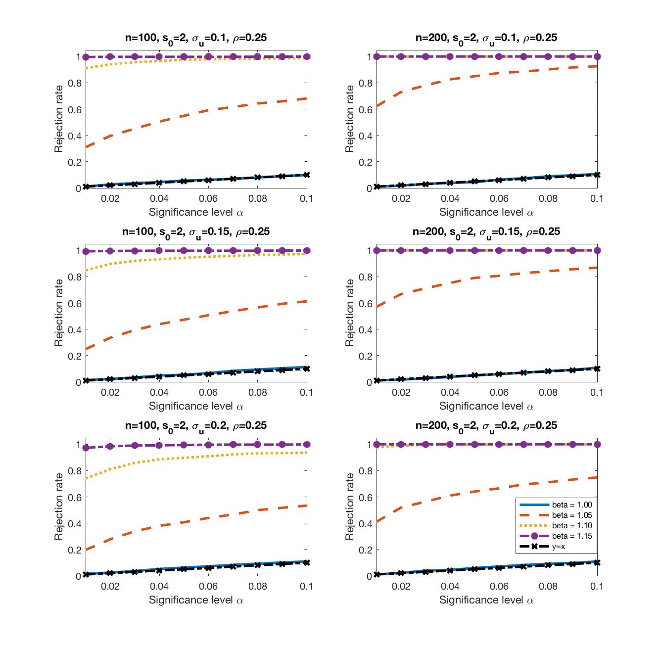
Figure 1: Power of the proposed corrected decorrelated score test at different significance levels in scenario 1 with $\rho=0.25$

Table 2: Performance of the one-step estimator $\widehat{\beta}$

		Scenario 1				Scenario 2
		$\rho=0.25$		$\rho=0.5$		$\rho=0.25$		$\rho=0.5$
$\sigma_{U}$		$n=100$	$n=200$	$n=100$	$n=200$	$n=100$	$n=200$	$n=100$	$n=200$
0.1	Mean	1.0008	1.0000	1.0010	1.0001	1.0008	1.0000	1.0003	0.9996
	Est sd	0.0237	0.0163	0.0259	0.0177	0.0235	0.0162	0.0257	0.0177
	Emp sd	0.0246	0.0167	0.0259	0.0185	0.0246	0.0167	0.0260	0.0185
	Emp cvg	$94.1\%$	$94.6\%$	$93.6\%$	$93.8\%$	$93.9\%$	$94.7\%$	$93.7\%$	$93.6\%$
0.15	Mean	1.0024	1.0011	1.0031	1.0012	1.0024	1.0011	1.0028	1.0009
	Est sd	0.0268	0.0183	0.0294	0.0199	0.0267	0.0183	0.0292	0.0199
	Emp sd	0.0279	0.0183	0.0299	0.0204	0.0270	0.0184	0.0302	0.0204
	Emp cvg	$94.2\%$	$94.9\%$	$93.3\%$	$94.0\%$	$94.6\%$	$94.7\%$	$93.4\%$	$93.7\%$
0.2	Mean	1.0049	1.0015	1.0062	1.0024	1.0085	1.0016	1.0061	1.0021
	Est sd	0.0309	0.0211	0.0341	0.0230	0.0313	0.0211	0.0339	0.0229
	Emp var	0.0324	0.0217	0.0355	0.0234	0.0333	0.0218	0.0359	0.0234
	Emp cvg	$94.1\%$	$94.1\%$	$93.0\%$	$93.5\%$	$92.9\%$	$93.9\%$	$92.2\%$	$93.2\%$

• In Table 2, “Est sd” denotes the mean of 1000 estimated asymptotic standard deviations; “Emp sd” denotes the empirical standard deviation of 1000 estimates; “Emp cvg” denotes the empirical coverage of the estimated $95\%$ CI for ${\boldsymbol{\beta}}_{0}$.

4.2 Real Data Analysis

We illustrate the proposed procedure via an empirical analysis of a data set analyzed in Chu et al. (2016). The data set was collected in a clinical trial designed to determine the long-term effects of different inhaled treatments for mild to moderate childhood asthma, where phenotypic information and genome-wide SNP data are accessible. The FEV1/FVC ratio is an important index used in diagnosis of obstructive and restrictive lung disease, which represents the proportion of a person’s vital capability to expire in the first second of forced expiration to the full vital capacity. We are interested in understanding how this ratio, often measured with errors, together with basic demographic variables and SNPs would affect the severity of asthma symptoms in children.

Here we focus on $n=199$ subjects in the nedocromil treatment group, each had four clinical visits over 8 months. Exploratory data analysis was conducted on the four measurements of FEV1/FVC ratio, and no visible time trend was detected. The response variable $Y_{i}$ is the average asthma symptoms (amsys). We let $X_{i}$ be the unobserved FEV1/FVC ratio and $W_{i}$ be the average of four measurements with homoscedastic measurement errors. Standard deviation and the fourth moment of measurement error $U_{i}$ are estimated using the four measurements for each subject based on the fact that $W_{ik}-W_{ij}=U_{ik}-U_{ij}$, $\hbox{var}(U_{ik}-U_{ij})=2\sigma_{U}^{2}$, and $E(U_{i}^{4})=[E\{(U_{ik}-U_{ij})^{4}\}-6\sigma_{U}^{4}]/2$ for $i=1,\dots n$ and $j,k=1,\dots,4$. Note that we do not need to assume the normality of measurement errors here. The estimated values are $\widehat{\sigma}_{U}=0.4625$ and $\widehat{E}(U_{i}^{4})=0.1719$. The error-free variables ${\bf Z}_{i}$ are gender, age at baseline and 676 SNPs screened based on minor allele frequency (MAF). Here we treat SNPs as continuous variables by assuming that having two of the minor alleles has twice the effect on the phenotype as having one of the minor alleles, and zero means no effect.

Our goal is to first select significant variables among $p=679$ variables in model (2), estimate the corresponding coefficients and then make inference for the error-prone variable FEV1/FVC ratio based on the proposed corrected decorrelated score test and the asymptotic properties of the one-step estimator. For the initial CoCoLasso estimator $\widetilde{\boldsymbol{\theta}}$, the tuning parameter $\lambda$ is selected by cross validation with the criterion proposed in Datta et al. (2017). We find that besides FEV1/FVC ratio which is of interest, seven SNPs are selected. Detailed information about the selected SNPs is given in Table 3.

Table 3: Information about the seven SNPs selected by CoCoLasso method

	${\rm SNP}_{1}$	${\rm SNP}_{2}$	${\rm SNP}_{3}$	${\rm SNP}_{4}$	${\rm SNP}_{5}$	${\rm SNP}_{6}$	${\rm SNP}_{7}$
SNP name	rs2830066	rs11798747	rs6961655	rs4432291	rs6860832	rs699770	rs4520841
Chromosome	21	X	7	17	5	1	16
Chr.position	26121885	18889776	136422490	72610903	8451644	119318352	26088794
Coefficient	0.0143	-0.0125	-0.0118	-0.0092	-0.0056	-0.0046	-0.0025

Under the null hypothesis $H_{0}:\beta_{0}=0$, the corrected decorrelated score test statistic $\widehat{T}_{n}=4.9806$. Hence, we reject the null hypothesis. The CoCoLasso estimate for $\beta$ is $-0.0654$, while the one-step estimate is $-0.1101$ with confidence interval $(-0.1508,-0.0693)$. The negativeness of $\widehat{\beta}$ verifies the fact that the lower the FEV1/FVC ratio, the severer the obstruction of air escaping from the lungs.

Throughout the data analysis, we estimated the second and fourth moments of the measurement error using the four measurements of each subject. Because of the independent error assumption, $U_{ik}+U_{ij}$ is uncorrelated to $U_{ij}-U_{ik}$. Recall that the $W_{i}$ relies on $U_{ik}+U_{ij}$, while the error moment estimates are based on $U_{ij}-U_{ik}$. Under normality assumption, the standard errors of the two moment estimates do not affect the performance of our proposed inference procedure.

5 Discussion

In this paper, we have proposed an inference procedure for high-dimensional linear measurement error models based on corrected decorrelated score functions. With the decorrelation operation, our corrected score test statistic $\widehat{T}_{n}$ is asymptotically normal and retains power under the local alternatives around 0. Further, the convergence rate of the one-step estimator $\widehat{\boldsymbol{\beta}}$ has significantly improved compared to that of the initial estimator and achieves the semiparametric efficiency. Here we have assumed that the variance and the fourth moments of the measurement error are known. The framework in this paper still works if we treat $\sigma_{U}^{2}$ and $E(U_{i}^{4})$ as nuisance parameters and then conduct decorrelation. Specifically, the new nuisance parameters are $({\boldsymbol{\gamma}}^{\rm T},\sigma_{U}^{2},E(U_{i}^{4}))$. Note that we do not impose any penalty on $\sigma_{U}^{2}$ and $E(U_{i}^{4})$.

One further research direction is to develop inference procedures when the number of covariates with measurement errors diverges with sample size $n$. Another possible consideration is to relax the sparsity assumption on $\boldsymbol{\omega}$. That is, extend the theory to cases where the ordered entries of $\boldsymbol{\omega}$ decay at a certain rate.

Appendix A: Four technical Conditions

Lemma 3.

Recall that $S^{\prime}=\rm{supp}(\boldsymbol{\omega})$ and $|S^{\prime}|=s^{\prime}$. Let $\lambda^{\prime}=C_{\lambda^{\prime}}\sqrt{n^{-1}{\rm log}p}$. The Dantzig type estimator $\widehat{\boldsymbol{\omega}}$ satisfies $\|\widehat{\boldsymbol{\omega}}-\boldsymbol{\omega}\|_{1}=O_{P}(s^{\prime}\sqrt{n^{-1}{\rm log}{p}})$, when $C_{\lambda^{\prime}}>\sqrt{2K_{5}/C^{\prime\prime}}$. Here $C^{\prime\prime}$ is a universal constant and $K_{5}=2K(K+K_{U}+KK_{\omega})$.

Lemma 4.

Let $\boldsymbol{\nu}=(1,-\boldsymbol{\omega}^{\rm T})^{\rm T}$. The gradient and Hessian of the corrected loss function (3) satisfy $\|{\bf S}_{{\boldsymbol{\theta}}}({\boldsymbol{\theta}}_{0})\|_{\infty}=O_{p}(\sqrt{n^{-1}{\rm log}{p}})$ and $\|\boldsymbol{\nu}^{\rm T}\nabla{\bf S}_{{\boldsymbol{\theta}}}({\boldsymbol{\theta}}_{0})-E\{\boldsymbol{\nu}^{\rm T}\nabla{\bf S}_{{\boldsymbol{\theta}}}({\boldsymbol{\theta}}_{0})\}\|_{\infty}=O_{P}(\sqrt{n^{-1}{\rm log}{p}})$.

Lemma 5.

Let $\widetilde{\boldsymbol{\theta}}_{H_{0}}=(\beta^{*},\widetilde{\boldsymbol{\gamma}}^{\rm T})^{\rm T}$, $\widehat{\boldsymbol{\nu}}=(1,-\widehat{\boldsymbol{\omega}}^{\rm T})^{\rm T}$. Assume that

$$\frac{s_{0}(s^{\prime}\vee s_{0}){\rm log}p}{\sqrt{n}}=o(1).$$

Then $\boldsymbol{\nu}^{\rm T}\{{\bf S}_{{\boldsymbol{\theta}}}(\widecheck{{\boldsymbol{\theta}}})-{\bf S}_{{\boldsymbol{\theta}}}({\boldsymbol{\theta}}_{0})-\nabla{\bf S}_{{\boldsymbol{\theta}}}({\boldsymbol{\theta}}_{0})(\widecheck{{\boldsymbol{\theta}}}-{\boldsymbol{\theta}}_{0})\}=0$, and $(\widehat{\boldsymbol{\nu}}-\boldsymbol{\nu})^{\rm T}\{{\bf S}_{{\boldsymbol{\theta}}}(\widecheck{{\boldsymbol{\theta}}})-{\bf S}_{{\boldsymbol{\theta}}}({\boldsymbol{\theta}}_{0})\}=o_{P}(n^{-1/2})$, for both $\widecheck{{\boldsymbol{\theta}}}=\widetilde{\boldsymbol{\theta}}_{H_{0}}$ and $\widecheck{{\boldsymbol{\theta}}}=\widetilde{\boldsymbol{\theta}}$.

Lemma 6.

When (2) does not degenerate, i.e., the corrected decorrelated score function $S({\boldsymbol{\theta}})\not\equiv 0$ a.s., then

$$\sqrt{n}\boldsymbol{\nu}^{\rm T}{\bf S}_{{\boldsymbol{\theta}}}({\boldsymbol{\theta}}_{0})(\sigma^{2}_{\beta|{\boldsymbol{\gamma}},0})^{-1/2}\to N(0,1)$$

in distribution. Here $\sigma^{2}_{\beta|{\boldsymbol{\gamma}},0}=(\sigma_{\epsilon}^{2}+\beta_{0}^{2}\sigma_{U}^{2})\{1-\boldsymbol{\omega}^{\rm T}E(X_{i}{\bf Z}_{i})\}+\beta_{0}^{2}E(U_{i}^{4})+\sigma_{\epsilon}^{2}\sigma_{U}^{2}-\beta_{0}^{2}\sigma_{U}^{4}$ by (4) and (5), and $\sigma^{2}_{\beta|{\boldsymbol{\gamma}},0}\geq C$ for some positive constant $C$.

Lemma 3, together with Lemma 1, states the consistency properties for initial estimators $\widetilde{\boldsymbol{\theta}}$ and $\widehat{\boldsymbol{\omega}}$, which are crucial to the asymptotic performance of our corrected test statistic and one-step estimator. Lemma 4 and Lemma 5 describe the concentration properties of the gradient and Hessian of the corrected loss function (3), and its local smoothness properties, respectively. For high-dimensional random designs, it is important to quantify the distance between sample level statistic and its corresponding population level value, especially for critical statistics like the score function and the Hessian matrix. For local smoothness, Ning et al. (2017) require $(s_{0}\vee s^{\prime})n^{-1/2}{\rm log}p=o(1)$. However, using CoCoLasso estimator as the initial estimator, we need a stronger condition on dimensionality and sparsity to guarantee the $n^{-1/2}$ rate local smoothness of the corrected loss function. Lemma 6 is the central limit theorem for corrected decorrelated sore function $S({\boldsymbol{\theta}}_{0})$, which is a linear combination of $S_{{\boldsymbol{\theta}}}({\boldsymbol{\theta}}_{0})$. Because we define the score function as the gradient of the corrected loss function, which is different from negative log-likelihood, the variance $\sigma^{2}_{\beta\mid{\boldsymbol{\gamma}},0}$ of $S({\boldsymbol{\theta}}_{0})$ has relatively complex form. Detailed proofs of the four lemmas are given in Appendices F.1, F.2, F.3 and F.4, respectively, in supplementary materials.

Appendix B: Proofs Regarding Score Test Statistic

B.1 Proof of Theorem 1

Proof.

Recall that $\widetilde{\boldsymbol{\theta}}_{H_{0}}=(\beta^{*},\widetilde{\boldsymbol{\gamma}}^{\rm T})^{\rm T}$, $\widehat{\boldsymbol{\nu}}=(1,-\widehat{\boldsymbol{\omega}}^{\rm T})^{\rm T}$ and $\boldsymbol{\nu}=(1,-\boldsymbol{\omega}^{\rm T})^{\rm T}$. We have

$$\sqrt{n}|\widehat{S}(\widetilde{\boldsymbol{\theta}}_{H_{0}})-S({\boldsymbol{\theta}}_{0})|$$

$$= \sqrt{n}|\widehat{\boldsymbol{\nu}}^{\rm T}{\bf S}_{{\boldsymbol{\theta}}}(\widetilde{\boldsymbol{\theta}}_{H_{0}})-\boldsymbol{\nu}^{\rm T}{\bf S}_{{\boldsymbol{\theta}}}({\boldsymbol{\theta}}_{0})|$$

$$\leq \sqrt{n}|\boldsymbol{\nu}^{\rm T}\{{\bf S}_{{\boldsymbol{\theta}}}(\widetilde{\boldsymbol{\theta}}_{H_{0}})-S_{{\boldsymbol{\theta}}}({\boldsymbol{\theta}}_{0})\}|+\sqrt{n}|(\widehat{\boldsymbol{\nu}}-\boldsymbol{\nu})^{\rm T}{\bf S}_{{\boldsymbol{\theta}}}(\widetilde{\boldsymbol{\theta}}_{H_{0}})|$$

$$= D_{1}+D_{2},$$

where $D_{1}\equiv\sqrt{n}|\boldsymbol{\nu}^{\rm T}\{{\bf S}_{{\boldsymbol{\theta}}}(\widetilde{\boldsymbol{\theta}}_{H_{0}})-S_{{\boldsymbol{\theta}}}({\boldsymbol{\theta}}_{0})\}|$ and $D_{2}\equiv\sqrt{n}|(\widehat{\boldsymbol{\nu}}-\boldsymbol{\nu})^{\rm T}{\bf S}_{{\boldsymbol{\theta}}}(\widetilde{\boldsymbol{\theta}}_{H_{0}})|$. Since the corrected loss function (3) is a quadratic function of ${\boldsymbol{\theta}}$, by Lemma 5, we have

$$|D_{1}| = \sqrt{n}|\boldsymbol{\nu}^{\rm T}\nabla{\bf S}_{{\boldsymbol{\theta}}}({\boldsymbol{\theta}}_{0})(\widetilde{\boldsymbol{\theta}}_{H_{0}}-{\boldsymbol{\theta}}_{0})|$$ (11)

$$= \sqrt{n}|\boldsymbol{\nu}^{\rm T}\nabla{\bf S}_{{\boldsymbol{\theta}}}({\boldsymbol{\theta}}_{0})(0,\widetilde{\boldsymbol{\gamma}}^{\rm T}-{\boldsymbol{\gamma}}_{0}^{\rm T})^{\rm T}|$$

$$\leq \sqrt{n}\|\widetilde{\boldsymbol{\gamma}}-{\boldsymbol{\gamma}}_{0}\|_{1}\|\widehat{\bf\Sigma}_{12}-\boldsymbol{\omega}^{\rm T}\widehat{\bf\Sigma}_{22}\|_{\infty}$$

$$= \sqrt{n}\|\widetilde{\boldsymbol{\theta}}_{H_{0}}-{\boldsymbol{\theta}}_{0}\|_{1}\|\widehat{\bf\Sigma}_{12}-\boldsymbol{\omega}^{\rm T}\widehat{\bf\Sigma}_{22}\|_{\infty}$$

$$= \sqrt{n}\|\widetilde{\boldsymbol{\theta}}_{H_{0}}-{\boldsymbol{\theta}}_{0}\|_{1}\|\widehat{\bf\Sigma}_{12}-\boldsymbol{\omega}^{\rm T}\widehat{\bf\Sigma}_{22}-E\{\widehat{\bf\Sigma}_{12}-\boldsymbol{\omega}^{\rm T}\widehat{\bf\Sigma}_{22}\}\|_{\infty}$$

$$+\sqrt{n}\|\widetilde{\boldsymbol{\theta}}_{H_{0}}-{\boldsymbol{\theta}}_{0}\|_{1}\|E\{\widehat{\bf\Sigma}_{12}-\boldsymbol{\omega}^{\rm T}\widehat{\bf\Sigma}_{22}\}\|_{\infty}$$

$$= \sqrt{n}\|\widetilde{\boldsymbol{\theta}}_{H_{0}}-{\boldsymbol{\theta}}_{0}\|_{1}\|\widehat{\bf\Sigma}_{12}-\boldsymbol{\omega}^{\rm T}\widehat{\bf\Sigma}_{22}-E\{\widehat{\bf\Sigma}_{12}-\boldsymbol{\omega}^{\rm T}\widehat{\bf\Sigma}_{22}\}\|_{\infty}$$

$$\leq \sqrt{n}\|\widetilde{\boldsymbol{\theta}}_{H_{0}}-{\boldsymbol{\theta}}_{0}\|_{1}\|\boldsymbol{\nu}^{\rm T}\nabla{\bf S}_{{\boldsymbol{\theta}}}({\boldsymbol{\theta}}_{0})-E\{\boldsymbol{\nu}^{\rm T}\nabla{\bf S}_{{\boldsymbol{\theta}}}({\boldsymbol{\theta}}_{0})\}\|_{\infty}.$$

In the above derivation, we used the fact that $\nabla{\bf S}_{{\boldsymbol{\theta}}}(\theta_{0})=\widehat{\bf\Sigma}$, and under $H_{0}$ the first element of $\widetilde{\boldsymbol{\theta}}_{H_{0}}-{\boldsymbol{\theta}}_{0}$ is $0$. In addition, $\boldsymbol{\omega}^{\rm T}=E(W_{i}{\bf Z}_{i}^{\rm T})E({\bf Z}_{i}{\bf Z}_{i}^{\rm T})^{-1}$, and hence

$$E(\widehat{\bf\Sigma}_{12}-\boldsymbol{\omega}^{\rm T}\widehat{\bf\Sigma}_{22})=E(W_{i}{\bf Z}_{i}^{\rm T})-\boldsymbol{\omega}^{\rm T}E({\bf Z}_{i}{\bf Z}_{i}^{\rm T})={\bf 0}.$$

By Lemmas 1 and 4, we have $D_{1}\leq O_{P}\left\{s_{0}^{2}\sqrt{n^{-1}{\rm log}p}\cdot\sqrt{{\rm log}p}\right\}=o_{P}(1)$.

For $D_{2}$, Lemma 5 yields

$$|D_{2}| \leq \sqrt{n}|(\widehat{\boldsymbol{\nu}}-\boldsymbol{\nu})^{\rm T}{\bf S}_{{\boldsymbol{\theta}}}({\boldsymbol{\theta}}_{0})|+\sqrt{n}|(\widehat{\boldsymbol{\nu}}-\boldsymbol{\nu})^{\rm T}\{{\bf S}_{{\boldsymbol{\theta}}}(\widetilde{\boldsymbol{\theta}}_{H_{0}})-{\bf S}_{{\boldsymbol{\theta}}}({\boldsymbol{\theta}}_{0})\}|$$

$$\leq \sqrt{n}|(\widehat{\boldsymbol{\nu}}-\boldsymbol{\nu})^{\rm T}{\bf S}_{{\boldsymbol{\theta}}}({\boldsymbol{\theta}}_{0})|+o_{P}(1)$$

$$\leq \sqrt{n}\|\widehat{\boldsymbol{\nu}}-\boldsymbol{\nu}\|_{1}\|{\bf S}_{{\boldsymbol{\theta}}}({\boldsymbol{\theta}}_{0})\|_{\infty}+o_{P}(1).$$

By Lemmas 3 and 4, we have $|D_{2}|\leq O_{P}\left\{s^{\prime}\sqrt{n^{-1}{\rm log}p}\cdot\sqrt{{\rm log}p}\right\}+o_{P}(1)=o_{P}(1)$. Hence, we have $\sqrt{n}|\widehat{S}(\widetilde{\boldsymbol{\theta}}_{H_{0}})-S({\boldsymbol{\theta}}_{0})|=o_{P}(1)$. Since $\sigma^{2}_{\beta|{\boldsymbol{\gamma}},0}>0$, we obtain that

$$\sqrt{n}\mid\widehat{S}(\widetilde{\boldsymbol{\theta}}_{H_{0}})(\sigma^{2}_{\beta|{\boldsymbol{\gamma}},0})^{-1/2}-S({\boldsymbol{\theta}}_{0})(\sigma^{2}_{\beta|{\boldsymbol{\gamma}},0})^{-1/2}\mid=o_{P}(1).$$

By Lemma 6, $\sqrt{n}S({\boldsymbol{\theta}}_{0})(\sigma^{2}_{\beta|{\boldsymbol{\gamma}},0})^{-1/2}=\sqrt{n}\boldsymbol{\nu}^{\rm T}{\bf S}_{\boldsymbol{\theta}}({\boldsymbol{\theta}}_{0})(\sigma^{2}_{\beta|{\boldsymbol{\gamma}},0})^{-1/2}\to N(0,1)$ in distribution. Applying the Slutsky’s theorem, we hence get $\sqrt{n}\widehat{S}(\beta^{*},\widetilde{\boldsymbol{\gamma}})(\sigma^{2}_{\beta|{\boldsymbol{\gamma}},0})^{-1/2}\to N(0,1)$ in distribution under null hypothesis. This completes the proof. ∎

B.2 Proof of Corollary 1

Proof.

Recall that $\widehat{T}_{n}=n^{1/2}\widehat{S}(\beta^{*},\widetilde{\boldsymbol{\gamma}})(\widehat{\sigma}_{\beta\mid{\boldsymbol{\gamma}},H_{0}}^{2})^{-1/2}$. Let $T_{n}=n^{1/2}\widehat{S}(\beta^{*},\widetilde{\boldsymbol{\gamma}})(\sigma_{\beta\mid{\boldsymbol{\gamma}},0}^{2})^{-1/2}$. Then

$$\widehat{T}_{n}-T_{n}=T_{n}\left(\frac{\sigma_{\beta\mid{\boldsymbol{\gamma}},0}}{\widehat{\sigma}_{\beta\mid{\boldsymbol{\gamma}},H_{0}}}-1\right).$$

In Theorem 1, we have proved that $T_{n}\to N(0,1)$ in distribution, as $n\to\infty$. It remains to show that $\sigma_{\beta\mid{\boldsymbol{\gamma}},0}/\widehat{\sigma}_{\beta\mid{\boldsymbol{\gamma}},H_{0}}-1=o_{p}(1)$. We start from deriving the bound of $|\widehat{\sigma}_{\beta\mid{\boldsymbol{\gamma}},H_{0}}^{2}-\sigma_{\beta\mid{\boldsymbol{\gamma}},0}^{2}|$. Recall that

$$\widehat{\sigma}_{\beta\mid{\boldsymbol{\gamma}},H_{0}}^{2} = (\widetilde{\sigma}_{\epsilon,H_{0}}^{2}+\beta^{*2}\sigma_{U}^{2})(1-\widehat{\boldsymbol{\omega}}^{\rm T}\widehat{\bf\Sigma}_{21})+\beta^{*2}E(U_{i}^{4})+\widetilde{\sigma}_{\epsilon,H_{0}}^{2}\sigma_{U}^{2}-\beta^{*2}\sigma_{U}^{4},$$

$$\sigma_{\beta\mid{\boldsymbol{\gamma}},0}^{2} = (\sigma_{\epsilon}^{2}+\beta_{0}^{2}\sigma_{U}^{2})\{1-\boldsymbol{\omega}^{\rm T}E(X_{i}{\bf Z}_{i})\}+\beta_{0}^{2}E(U_{i}^{4})+\sigma_{\epsilon}^{2}\sigma_{U}^{2}-\beta_{0}^{2}\sigma_{U}^{4}.$$

Since $\beta_{0}=\beta^{*}$ under null hypothesis, then we have

$$\widehat{\sigma}_{\beta\mid{\boldsymbol{\gamma}},H_{0}}^{2}-\sigma_{\beta\mid{\boldsymbol{\gamma}},0}^{2} = (\widetilde{\sigma}_{\epsilon,H_{0}}^{2}-\sigma_{\epsilon}^{2})\sigma_{U}^{2}+\beta_{0}^{2}\sigma_{U}^{2}\{\boldsymbol{\omega}^{\rm T}E(X_{i}{\bf Z}_{i})-\widehat{\boldsymbol{\omega}}^{\rm T}\widehat{\bf\Sigma}_{21}\}$$

$$+ \widetilde{\sigma}_{\epsilon,H_{0}}^{2}(1-\widehat{\boldsymbol{\omega}}^{\rm T}\widehat{\bf\Sigma}_{21})-\sigma_{\epsilon}^{2}\{1-\boldsymbol{\omega}^{\rm T}E(X_{i}{\bf Z}_{i})\}.$$

Let $D_{1}=(\widetilde{\sigma}_{\epsilon,H_{0}}^{2}-\sigma_{\epsilon}^{2})\sigma_{U}^{2}$, $D_{2}=\beta_{0}^{2}\sigma_{U}^{2}\{\boldsymbol{\omega}^{\rm T}E(X_{i}{\bf Z}_{i})-\widehat{\boldsymbol{\omega}}^{\rm T}\widehat{\bf\Sigma}_{21}\}$ and $D_{3}=\widetilde{\sigma}_{\epsilon,H_{0}}^{2}(1-\widehat{\boldsymbol{\omega}}^{\rm T}\widehat{\bf\Sigma}_{21})-\sigma_{\epsilon}^{2}\{1-\boldsymbol{\omega}^{\rm T}E(X_{i}{\bf Z}_{i})\}$. For term $D_{1}$, recall that

$$\widetilde{\sigma}_{\epsilon,H_{0}}^{2} = n^{-1}\sum_{i=1}^{n}(Y_{i}-\beta^{*}W_{i})^{2}-n^{-1}\sum_{i=1}^{n}(\widetilde{\boldsymbol{\gamma}}^{\rm T}{\bf Z}_{i})^{2}-\beta^{*2}\sigma_{U}^{2},$$

$$\sigma_{\epsilon}^{2} = E\{(Y_{i}-\beta_{0}W_{i})^{2}\}-E\{({\boldsymbol{\gamma}}_{0}^{\rm T}{\bf Z}_{i})^{2}\}-\beta_{0}^{2}\sigma_{U}^{2}.$$

Then we have

$$\widetilde{\sigma}_{\epsilon,H_{0}}^{2}-\sigma_{\epsilon}^{2}$$

$$= n^{-1}\sum_{i=1}^{n}(Y_{i}-\beta^{*}W_{i})^{2}-E\{(Y_{i}-\beta_{0}W_{i})^{2}\}-\left[n^{-1}\sum_{i=1}^{n}(\widetilde{\boldsymbol{\gamma}}^{\rm T}{\bf Z}_{i})^{2}-E\{({\boldsymbol{\gamma}}_{0}^{\rm T}{\bf Z}_{i})^{2}\}\right]$$

$$= n^{-1}\sum_{i=1}^{n}(Y_{i}-\beta_{0}W_{i})^{2}-E\{(Y_{i}-\beta_{0}W_{i})^{2}\}-\left[n^{-1}\sum_{i=1}^{n}(\widetilde{\boldsymbol{\gamma}}^{\rm T}{\bf Z}_{i})^{2}-E\{({\boldsymbol{\gamma}}_{0}^{\rm T}{\bf Z}_{i})^{2}\}\right].$$

First, by triangle inequality and Assumption 1, we know

$$\|{\boldsymbol{\gamma}}_{0}^{\rm T}{\bf Z}_{i}\|_{\psi_{2}}\leq\sum_{j=1}^{p-1}|\gamma_{0j}|\|{\bf Z}_{ij}\|_{\psi_{2}}\leq K\|{\boldsymbol{\gamma}}_{0}\|_{1}\leq s_{0}KK_{0}.$$

Then we have

$$\|s_{0}^{-2}(Y_{i}-\beta_{0}W_{i})^{2}\|_{\psi_{1}} = \|s_{0}^{-2}({\boldsymbol{\gamma}}_{0}^{\rm T}{\bf Z}_{i}+\epsilon_{i}-\beta_{0}U_{i})^{2}\|_{\psi_{1}}$$

$$\leq 2\|s_{0}^{-1}({\boldsymbol{\gamma}}_{0}^{\rm T}{\bf Z}_{i}+\epsilon_{i}-\beta_{0}U_{i})\|_{\psi_{2}}^{2}$$

$$\leq 2\left(\|s_{0}^{-1}{\boldsymbol{\gamma}}_{0}{\bf Z}_{i}\|_{\psi_{2}}+\|s_{0}^{-1}\epsilon_{i}\|_{\psi_{2}}+\|s_{0}^{-1}\beta_{0}U_{i}\|_{\psi_{2}}\right)^{2}$$

$$\leq 2(K_{0}K+s_{0}^{-1}K_{\epsilon}+s_{0}^{-1}|\beta_{0}|K_{U})^{2}$$

$$\leq K_{8},$$

where $K_{8}$ is a finite constant. Then by Bernstein inequality, for any $t>0$ we have

$$\Pr\left(s_{0}^{-2}\left|n^{-1}\sum_{i=1}^{n}(Y_{i}-\beta_{0}W_{i})^{2}-E\{(Y_{i}-\beta_{0}W_{i})^{2}\}\right|\geq t\right)\leq 2\exp\left\{-C^{\prime\prime}\min\left(\frac{t^{2}}{4K_{8}^{2}},\frac{t}{2K_{8}}\right)n\right\}.$$

Let $t=\sqrt{n^{-1}{\rm log}p}$. Then for $n$ large enough, we have

$$\Pr\left(\left|n^{-1}\sum_{i=1}^{n}(Y_{i}-\beta_{0}W_{i})^{2}-E\{(Y_{i}-\beta_{0}W_{i})^{2}\}\right|\leq s_{0}^{2}\sqrt{n^{-1}{\rm log}p}\right)\geq 1-2\exp\left(\frac{-C^{\prime\prime}{\rm log}p}{4K_{8}^{2}}\right).$$

Thus,

$$\left|n^{-1}\sum_{i=1}^{n}(Y_{i}-\beta_{0}W_{i})^{2}-E\{(Y_{i}-\beta_{0}W_{i})^{2}\}\right|\leq s_{0}^{2}\sqrt{n^{-1}{\rm log}p}$$ (12)

with probability tending to $1$. Note that under the condition given in Lemma 3, $s_{0}^{2}\sqrt{n^{-1}{\rm log}p}=o(1)$. For term $n^{-1}\sum_{i=1}^{n}(\widetilde{\boldsymbol{\gamma}}^{\rm T}{\bf Z}_{i})^{2}-E\{({\boldsymbol{\gamma}}_{0}^{\rm T}{\bf Z}_{i})^{2}\}$, we first have

$$\left|n^{-1}\sum_{i=1}^{n}(\widetilde{\boldsymbol{\gamma}}^{\rm T}{\bf Z}_{i})^{2}-E\{({\boldsymbol{\gamma}}_{0}^{\rm T}{\bf Z}_{i})^{2}\}\right|$$

$$\leq \left|n^{-1}\sum_{i=1}^{n}(\widetilde{\boldsymbol{\gamma}}^{\rm T}{\bf Z}_{i})^{2}-n^{-1}\sum_{i=1}^{n}({\boldsymbol{\gamma}}_{0}^{\rm T}{\bf Z}_{i})^{2}\right|+\left|n^{-1}\sum_{i=1}^{n}({\boldsymbol{\gamma}}_{0}^{\rm T}{\bf Z}_{i})^{2}-E\{({\boldsymbol{\gamma}}_{0}^{\rm T}{\bf Z}_{i})^{2}\}\right|$$

$$\leq \|\widetilde{\boldsymbol{\gamma}}-{\boldsymbol{\gamma}}_{0}\|_{1}\left\|n^{-1}\sum_{i=1}^{n}(\widetilde{\boldsymbol{\gamma}}+{\boldsymbol{\gamma}}_{0})^{\rm T}{\bf Z}_{i}{\bf Z}_{i}\right\|_{\infty}+\left|n^{-1}\sum_{i=1}^{n}({\boldsymbol{\gamma}}_{0}^{\rm T}{\bf Z}_{i})^{2}-E\{({\boldsymbol{\gamma}}_{0}^{\rm T}{\bf Z}_{i})^{2}\}\right|.$$

By triangle inequality, Lemma G.4 in supplementary materials and Lemma 1, we have

$$\|(\widetilde{\boldsymbol{\gamma}}+{\boldsymbol{\gamma}}_{0})^{\rm T}{\bf Z}_{i}Z_{ik}\|_{\psi_{1}} = \left\|\sum_{j=1}^{p-1}(\widetilde{\gamma}_{j}+\gamma_{0j})Z_{ij}Z_{ik}\right\|_{\psi_{1}}$$

$$\leq \sum_{j=1}^{p-1}|\widetilde{\gamma}_{j}+\gamma_{0j}|\|Z_{ij}Z_{ik}\|_{\psi_{1}}$$

$$\leq 2K^{2}\|\widetilde{\boldsymbol{\gamma}}+{\boldsymbol{\gamma}}_{0}\|_{1}$$

$$\leq 2K^{2}s_{0}(\|\widetilde{\boldsymbol{\gamma}}-{\boldsymbol{\gamma}}_{0}\|_{\infty}+2\|{\boldsymbol{\gamma}}_{0}\|_{\infty})$$

$$\leq 2K^{2}s_{0}(C_{\infty}C_{\lambda}s_{0}\sqrt{n^{-1}{\rm log}p}+2K_{0})$$

$$\leq 2K^{2}s_{0}K_{0}^{\prime},$$

with probability tending to 1, where $K_{0}^{\prime}$ is a constant. The third last inequality holds because the support of CoCoLasso estimate $\widetilde{\boldsymbol{\theta}}$ is a subset of the true support with probability going to 1. The second last inequality used result (b) in Lemma 2 and that $\|{\boldsymbol{\theta}}\|_{\infty}$ is bounded. Then $\|s_{0}^{-1}(\widetilde{\boldsymbol{\gamma}}+{\boldsymbol{\gamma}}_{0})^{\rm T}{\bf Z}_{i}Z_{ik}\|_{\psi_{1}}\leq 2K^{2}K_{0}^{\prime}<\infty$, for $k=1,\dots,p-1$. By the definition of sub-exponential norm, we know that $|E\{s_{0}^{-1}(\widetilde{\boldsymbol{\gamma}}+{\boldsymbol{\gamma}}_{0})^{\rm T}{\bf Z}_{i}Z_{ik}\}|$ is also finite. By Bernstein inequality and union bound inequality, for any $t>0$ we have

$$\Pr\left(\left\|n^{-1}\sum_{i=1}^{n}s_{0}^{-1}(\widetilde{\boldsymbol{\gamma}}+{\boldsymbol{\gamma}}_{0})^{\rm T}{\bf Z}_{i}{\bf Z}_{i}-E\{s_{0}^{-1}(\widetilde{\boldsymbol{\gamma}}+{\boldsymbol{\gamma}}_{0})^{\rm T}{\bf Z}_{i}{\bf Z}_{i}\}\right\|_{\infty}\geq t\right)$$

$$\leq 2p\exp\left\{-C^{\prime\prime}\min\left(\frac{t^{2}}{16K^{4}K_{0}^{\prime 2}},\frac{t}{4K^{2}K_{0}^{\prime}}\right)n\right\}.$$

Let $t=C\sqrt{n^{-1}{\rm log}p}$. Then for $n$ large enough, we have

$$\Pr\left(\left\|n^{-1}\sum_{i=1}^{n}s_{0}^{-1}(\widetilde{\boldsymbol{\gamma}}+{\boldsymbol{\gamma}}_{0})^{\rm T}{\bf Z}_{i}{\bf Z}_{i}-E\{s_{0}^{-1}(\widetilde{\boldsymbol{\gamma}}+{\boldsymbol{\gamma}}_{0})^{\rm T}{\bf Z}_{i}{\bf Z}_{i}\}\right\|_{\infty}\leq C\sqrt{n^{-1}{\rm log}p}\right)$$

$$\geq 1-2p\exp\left(\frac{-C^{\prime\prime}C^{2}{\rm log}p}{16K^{4}K_{0}^{\prime 2}}\right).$$

When $C^{\prime\prime}C^{2}/(16K^{4}K_{0}^{\prime})>1$, we have

$$\left\|n^{-1}\sum_{i=1}^{n}s_{0}^{-1}(\widetilde{\boldsymbol{\gamma}}+{\boldsymbol{\gamma}}_{0})^{\rm T}{\bf Z}_{i}{\bf Z}_{i}\right\|_{\infty}\leq\|E\{s_{0}^{-1}(\widetilde{\boldsymbol{\gamma}}+{\boldsymbol{\gamma}}_{0})^{\rm T}{\bf Z}_{i}{\bf Z}_{i}\}\|_{\infty}+C\sqrt{n^{-1}{\rm log}p}$$

with probability tending to $1$. Hence, we obtain that

$$\|\widetilde{\boldsymbol{\gamma}}-{\boldsymbol{\gamma}}_{0}\|_{1}\left\|n^{-1}\sum_{i=1}^{n}(\widetilde{\boldsymbol{\gamma}}+{\boldsymbol{\gamma}}_{0})^{\rm T}{\bf Z}_{i}{\bf Z}_{i}\right\|_{\infty} \leq s_{0}\|\widetilde{\boldsymbol{\theta}}-{\boldsymbol{\theta}}_{0}\|_{1}\left\{\|E\{s_{0}^{-1}(\widetilde{\boldsymbol{\gamma}}+{\boldsymbol{\gamma}}_{0})^{\rm T}{\bf Z}_{i}{\bf Z}_{i}\}\|_{\infty}+C\sqrt{n^{-1}{\rm log}p}\right\}$$

$$\leq 16s_{0}^{2}\lambda\kappa^{-1}\{\|E\{s_{0}^{-1}(\widetilde{\boldsymbol{\gamma}}+{\boldsymbol{\gamma}}_{0})^{\rm T}{\bf Z}_{i}{\bf Z}_{i}\}\|_{\infty}+C\sqrt{n^{-1}{\rm log}p}\}$$

$$\leq C_{1}s_{0}^{3}\sqrt{n^{-1}{\rm log}p},$$

for some constant $C_{1}$ with probability tending to $1$.

For term $\left|n^{-1}\sum_{i=1}^{n}({\boldsymbol{\gamma}}_{0}^{\rm T}{\bf Z}_{i})^{2}-E\{({\boldsymbol{\gamma}}_{0}^{\rm T}{\bf Z}_{i})^{2}\}\right|$, since $\|s_{0}^{-1}{\boldsymbol{\gamma}}_{0}^{\rm T}{\bf Z}_{i}\|_{\psi_{2}}\leq KK_{0}$, then $\|s_{0}^{-2}({\boldsymbol{\gamma}}_{0}^{\rm T}{\bf Z}_{i})^{2}\|_{\psi_{1}}\leq 2K^{2}K_{0}^{2}<\infty$ by Lemma G.4. By Bernstein inequality, for any $t>0$, we have

$$\Pr\left(\left|n^{-1}\sum_{i=1}^{n}s_{0}^{-2}({\boldsymbol{\gamma}}_{0}^{\rm T}{\bf Z}_{i})^{2}-E\{s_{0}^{-2}({\boldsymbol{\gamma}}_{0}^{\rm T}{\bf Z}_{i})^{2}\}\right|\geq t\right)\leq 2\exp\left\{-C^{\prime\prime}\min\left(\frac{t^{2}}{16K^{4}K_{0}^{4}},\frac{t}{4K^{2}K_{0}^{2}}\right)n\right\}.$$

Let $t=\sqrt{n^{-1}{\rm log}p}$, then for $n$ large enough we have

$$\Pr\left(\left|n^{-1}\sum_{i=1}^{n}({\boldsymbol{\gamma}}_{0}^{\rm T}{\bf Z}_{i})^{2}-E\{({\boldsymbol{\gamma}}_{0}^{\rm T}{\bf Z}_{i})^{2}\}\right|\leq s_{0}^{2}\sqrt{n^{-1}{\rm log}p}\right)\geq 1-2\exp\left(\frac{-C^{\prime\prime}{\rm log}p}{16K^{4}K_{0}^{4}}\right).$$

Hence, we obtain that

$$\left|n^{-1}\sum_{i=1}^{n}(\widetilde{\boldsymbol{\gamma}}^{\rm T}{\bf Z}_{i})^{2}-E\{({\boldsymbol{\gamma}}_{0}^{\rm T}{\bf Z}_{i})^{2}\}\right|\leq C_{1}s_{0}^{3}\sqrt{n^{-1}{\rm log}p}+s_{0}^{2}\sqrt{n^{-1}{\rm log}p}$$ (13)

with probability tending to $1$. Therefore, from (12) and (13), we obtain

$$|D_{1}| = |\widetilde{\sigma}_{\epsilon,H_{0}}^{2}-\sigma_{\epsilon}^{2}|\sigma_{U}^{2}$$ (14)

$$\leq \left(2s_{0}^{2}\sqrt{n^{-1}{\rm log}p}+C_{1}s_{0}^{3}\sqrt{n^{-1}{\rm log}p}\right)\sigma_{U}^{2}$$

$$\leq C_{2}s_{0}^{3}\sqrt{n^{-1}{\rm log}p}\sigma_{U}^{2},$$

with probability tending to $1$.

For term $D2$, by triangle inequality, we first have

$$|D_{2}| \leq \beta_{0}^{2}\sigma_{U}^{2}\{|\boldsymbol{\omega}^{\rm T}\{E(X_{i}{\bf Z}_{i})-\widehat{\bf\Sigma}_{21}\}|+|(\widehat{\boldsymbol{\omega}}-\boldsymbol{\omega})^{\rm T}\widehat{\bf\Sigma}_{21}|\}$$

$$\leq \beta_{0}^{2}\sigma_{U}^{2}\{\|\boldsymbol{\omega}\|_{1}\|\widehat{\bf\Sigma}_{21}-E(X_{i}{\bf Z}_{i})\|_{\infty}+\|\widehat{\boldsymbol{\omega}}-\boldsymbol{\omega}\|_{1}\|\widehat{\bf\Sigma}_{21}\|_{\infty}\}.$$

In the proof of Lemma 1, we have showed that $\{\widehat{\bf\Sigma}_{21}-E(X_{i}{\bf Z}_{i})\}_{j}$ is sub-exponential and $\|\{\widehat{\bf\Sigma}_{21}-E(X_{i}{\bf Z}_{i})\}_{j}\|_{\psi_{1}}\leq 4K^{2}$ for $j=1,\dots,p-1$. Then by Bernstein inequality, for any $t>0$ we have

$$\Pr\left(\|\widehat{\bf\Sigma}_{21}-E(X_{i}{\bf Z}_{i})\|_{\infty}\geq t\right)\leq 2(p-1)\exp\left\{-C^{\prime\prime}\min\left(\frac{t^{2}}{16K^{4}},\frac{t}{4K^{2}}\right)n\right\}.$$

Let $t=M\sqrt{n^{-1}{\rm log}p}$, where $M>0$. Then for any $\varepsilon>0$, there exists $M>\sqrt{16K^{4}/C^{\prime\prime}}$, such that

$$\Pr\left(\|\widehat{\bf\Sigma}_{21}-E(X_{i}{\bf Z}_{i})\|_{\infty}\geq M\sqrt{n^{-1}{\rm log}p}\right)\leq\varepsilon,$$ (15)

for $n$ large enough. Hence, $\|\widehat{\bf\Sigma}_{21}-E(X_{i}{\bf Z}_{i})\|_{\infty}=O_{P}(\sqrt{n^{-1}{\rm log}p})$. By Assumption 1, then we have

$$\|\boldsymbol{\omega}\|_{1}\|\widehat{\bf\Sigma}_{21}-E(X_{i}{\bf Z}_{i})\|_{\infty}\leq K_{\boldsymbol{\omega}}M\sqrt{n^{-1}{\rm log}p}\leq C_{3}\sqrt{n^{-1}{\rm log}p}$$

for some constant $C_{3}$, with probability tending to $1$. Here, $K_{\boldsymbol{\omega}}$ is a positive constant satisfying $\|E(X_{i}{\bf Z}_{i}^{\rm T})\{E({\bf Z}_{i}^{\otimes 2})\}^{-1}\|_{1}\leq K_{\boldsymbol{\omega}}$. Since the data is standardized, $|E(X_{i}Z_{ij})|=|{\rm cor}(X_{i},Z_{ij})|\leq 1$ for $j=1,\dots,p-1$. Then $\|E(X_{i}{\bf Z}_{i})\|_{\infty}\leq 1$. By (15), $\|\widehat{\bf\Sigma}_{21}\|_{\infty}\leq\|E(X_{i}{\bf Z}_{i})\|_{\infty}+M\sqrt{n^{-1}{\rm log}p}\leq 1+M\sqrt{n^{-1}{\rm log}p}$ for some constant $M$ and $n$ large enough, with probability tending to $1$. By Lemma 3, we have

$$\|\widehat{\boldsymbol{\omega}}-\boldsymbol{\omega}\|_{1}\|\widehat{\bf\Sigma}_{21}\|_{\infty}\leq\|\widehat{\boldsymbol{\omega}}-\boldsymbol{\omega}\|_{1}+\|\widehat{\boldsymbol{\omega}}-\boldsymbol{\omega}\|_{1}M\sqrt{n^{-1}{\rm log}p}\leq C_{4}s^{\prime}\sqrt{n^{-1}{\rm log}p}$$ (16)

for some constant $C_{4}$, with probability tending to $1$. Then we obtain

$$|D_{2}|\leq\beta_{0}^{2}\sigma_{U}^{2}(C_{3}+C_{4})s^{\prime}\sqrt{n^{-1}{\rm log}p}.$$ (17)

with probability tending to $1$.

For term $D3$, by triangle inequality, (14) and (17), we have

$$|D_{3}| \leq \widetilde{\sigma}_{\epsilon,H_{0}}^{2}|\boldsymbol{\omega}^{\rm T}E(X_{i}{\bf Z}_{i})-\widehat{\boldsymbol{\omega}}^{\rm T}\widehat{\bf\Sigma}_{21}|+|1-\boldsymbol{\omega}^{\rm T}E(X_{i}{\bf Z}_{i})|\cdot|\widetilde{\sigma}_{\epsilon,H_{0}}^{2}-\sigma_{\epsilon}^{2}|$$

$$\leq \widetilde{\sigma}_{\epsilon,H_{0}}^{2}(C_{3}+C_{4})s^{\prime}\sqrt{n^{-1}{\rm log}p}+|1-\boldsymbol{\omega}^{\rm T}E(X_{i}{\bf Z}_{i})|C_{2}s_{0}^{3}\sqrt{n^{-1}{\rm log}p}$$

$$\leq (\sigma_{\epsilon}^{2}+C_{2}s_{0}^{3}\sqrt{n^{-1}{\rm log}p})(C_{3}+C_{4})s^{\prime}\sqrt{n^{-1}{\rm log}p}+|1-\boldsymbol{\omega}^{\rm T}E(X_{i}{\bf Z}_{i})|C_{2}s_{0}^{3}\sqrt{n^{-1}{\rm log}p}$$

$$\leq C_{5}(s_{0}^{3}+s^{\prime})\sqrt{n^{-1}{\rm log}p}$$

with probability tending to $1$, where $C_{5}$ is a constant. Note that $|1-\boldsymbol{\omega}^{\rm T}E(X_{i}{\bf Z}_{i})|$ is bounded, because $\|\boldsymbol{\omega}\|_{1}\leq K_{\boldsymbol{\omega}}$ and $\|E(X_{i}{\bf Z}_{i})\|_{\infty}\leq 1$. Therefore,

$$\left|\widehat{\sigma}_{\beta\mid{\boldsymbol{\gamma}},H_{0}}^{2}-\sigma_{\beta\mid{\boldsymbol{\gamma}},0}^{2}\right|\leq|D_{1}|+|D_{2}|+|D_{3}|=O_{p}\{(s_{0}^{3}+s^{\prime})\sqrt{n^{-1}{\rm log}p}\}.$$

Since we assume that the true parameter $\sigma_{\beta\mid{\boldsymbol{\gamma}},0}^{2}$ is bounded away from $0$, $s_{0}^{3}\sqrt{n^{-1}{\rm log}p}=o(1)$ and $s^{\prime}\sqrt{n^{-1}{\rm log}p}=o(1)$, then

$$\left|\frac{\sigma_{\beta\mid{\boldsymbol{\gamma}},0}}{\widehat{\sigma}_{\beta\mid{\boldsymbol{\gamma}},H_{0}}}-1\right| = \frac{1}{\widehat{\sigma}_{\beta\mid{\boldsymbol{\gamma}},H_{0}}(\widehat{\sigma}_{\beta\mid{\boldsymbol{\gamma}},H_{0}}+\sigma_{\beta\mid{\boldsymbol{\gamma}},0})}|\sigma_{\beta\mid{\boldsymbol{\gamma}},0}^{2}-\widehat{\sigma}_{\beta\mid{\boldsymbol{\gamma}},H_{0}}^{2}|$$

$$\leq \widehat{\sigma}_{\beta\mid{\boldsymbol{\gamma}},H_{0}}^{-2}|\sigma_{\beta\mid{\boldsymbol{\gamma}},0}^{2}-\widehat{\sigma}_{\beta\mid{\boldsymbol{\gamma}},H_{0}}^{2}|$$

$$\leq C_{6}|\sigma_{\beta\mid{\boldsymbol{\gamma}},0}^{2}-\widehat{\sigma}_{\beta\mid{\boldsymbol{\gamma}},H_{0}}^{2}|,$$

for some constant $C_{6}$ with probability tending to $1$. Hence, $|\sigma_{\beta\mid{\boldsymbol{\gamma}},0}/\widehat{\sigma}_{\beta\mid{\boldsymbol{\gamma}},H_{0}}-1|=o_{p}(1)$ and $\widehat{T}_{n}\to N(0,1)$ in distribution as $n$ goes to infinity. ∎

B.3 Proof of Corollary 2

Proof.

Under local alternatives, we know $E\{S(\beta_{n},{\boldsymbol{\gamma}}_{0})\}=0$ and $\sqrt{n}\widehat{S}(\beta_{n},\widetilde{\boldsymbol{\gamma}})(\widehat{\sigma}^{2}_{\beta_{n}|{\boldsymbol{\gamma}}})^{-1/2}$ converges to standard normal distribution by Corollary 1. Then by Taylor expansion, we have

$$\widehat{T}_{n} = \frac{\sqrt{n}\widehat{S}(\beta_{n},\widetilde{\boldsymbol{\gamma}})}{\sqrt{\widehat{\sigma}^{2}_{\beta_{n}|{\boldsymbol{\gamma}}}}}+\left\{\frac{\partial\widehat{S}(\beta_{0n},\widetilde{\boldsymbol{\gamma}})}{\partial\beta_{0n}}\frac{1}{\sqrt{\widehat{\sigma}^{2}_{\beta_{0n}|{\boldsymbol{\gamma}}}}}-\frac{\widehat{S}(\beta_{0n},\widetilde{\boldsymbol{\gamma}})}{2(\widehat{\sigma}^{2}_{\beta_{0n}|{\boldsymbol{\gamma}}})^{3/2}}\right\}\sqrt{n}(\beta^{*}-\beta_{n})$$

$$= \frac{\sqrt{n}\widehat{S}(\beta_{n},\widetilde{\boldsymbol{\gamma}})}{\sqrt{\widehat{\sigma}^{2}_{\beta_{n}|{\boldsymbol{\gamma}}}}}+\left[E\left\{\frac{\partial S(\beta,{\boldsymbol{\gamma}}_{0})}{\partial\beta}\bigg{\arrowvert}_{\beta=\beta_{n}}\right\}\frac{1}{\sqrt{\sigma^{2}_{\beta_{n}|{\boldsymbol{\gamma}},0}}}-\frac{E\{S(\beta_{n},{\boldsymbol{\gamma}}_{0})\}}{2(\sigma^{2}_{\beta_{n}|{\boldsymbol{\gamma}},0})^{3/2}}\right]\sqrt{n}(\beta^{*}-\beta_{n})+o_{p}(1)$$

$$= \frac{\sqrt{n}\widehat{S}(\beta_{n},\widetilde{\boldsymbol{\gamma}})}{\sqrt{\widehat{\sigma}^{2}_{\beta_{n}|{\boldsymbol{\gamma}}}}}-hE\left\{\frac{\partial S(\beta,{\boldsymbol{\gamma}}_{0})}{\partial\beta}\bigg{\arrowvert}_{\beta=\beta_{n}}\right\}\frac{1}{\sqrt{\sigma^{2}_{\beta_{n}|{\boldsymbol{\gamma}},0}}}+o_{p}(1)$$

$$\to N\{-h(\sigma_{\beta}^{2})^{-1/2},1\}$$

in distribution, where $\beta_{0n}$ is between $\beta^{*}$ and $\beta_{n}$, and $\sigma^{2}_{\beta_{n}|{\boldsymbol{\gamma}},0}$ is the variance of the decorrelated score $S(\beta_{n},{\boldsymbol{\gamma}}_{0})$ under local alternatives. Therefore, the power function converges to $\Pr\{|Z-h(\sigma_{\beta}^{2})^{-1/2}|\geq Z_{\alpha/2}\}$, where $Z$ is a standard normal random variable. ∎

Appendix C: Proofs Regarding Confidence Interval

C.1 Proof of Theorem 2

Proof.

To prove the asymptotic normality of the one-step estimator $\widehat{\beta}$, we first show that $\{\partial\widehat{\bf S}(\beta,\widetilde{\boldsymbol{\gamma}})/\partial\beta\}|_{\beta=\widetilde{\beta}}=1-\widehat{\boldsymbol{\omega}}^{\rm T}\widehat{\bf\Sigma}_{21}$ is consistent for $E[\{\partial S(\beta,{\boldsymbol{\gamma}}_{0})/\partial\beta\}|_{\beta=\beta_{0}}]=1-\boldsymbol{\omega}^{\rm T}E(X_{i}{\bf Z}_{i})$. By triangle inequality, we have the following decomposition

$$|1-\boldsymbol{\omega}^{\rm T}E(X_{i}{\bf Z}_{i})-(1-\widehat{\boldsymbol{\omega}}^{\rm T}\widehat{\bf\Sigma}_{21})| = |\widehat{\boldsymbol{\omega}}^{\rm T}\widehat{\bf\Sigma}_{21}-\boldsymbol{\omega}^{\rm T}E(X_{i}{\bf Z}_{i})|$$

$$\leq |\boldsymbol{\omega}^{\rm T}\{\widehat{\bf\Sigma}_{21}-E(X_{i}{\bf Z}_{i})\}|+|(\widehat{\boldsymbol{\omega}}-\boldsymbol{\omega})^{\rm T}\widehat{\bf\Sigma}_{21}|$$

$$\leq \|\boldsymbol{\omega}\|_{1}\|\widehat{\bf\Sigma}_{21}-E(X_{i}{\bf Z}_{i})\|_{\infty}+\|\widehat{\boldsymbol{\omega}}-\boldsymbol{\omega}\|_{1}\|\widehat{\bf\Sigma}_{21}\|_{\infty}.$$

By (15), we know that $\|\widehat{\bf\Sigma}_{21}-E(X_{i}{\bf Z}_{i})\|_{\infty}=O_{P}(\sqrt{n^{-1}{\rm log}p})$. Since $\|\boldsymbol{\omega}\|_{1}\leq K_{\boldsymbol{\omega}}$, then $\|\boldsymbol{\omega}\|_{1}\|\widehat{\bf\Sigma}_{21}-E(X_{i}{\bf Z}_{i})\|_{\infty}=O_{P}(\sqrt{n^{-1}{\rm log}p})$. By (16), we have $\|\widehat{\boldsymbol{\omega}}-\boldsymbol{\omega}\|_{1}\|\widehat{\bf\Sigma}_{21}\|_{\infty}=O_{P}(s^{\prime}\sqrt{n^{-1}{\rm log}p})$. Hence, $|1-\boldsymbol{\omega}^{\rm T}E(X_{i}{\bf Z}_{i})-(1-\widehat{\boldsymbol{\omega}}^{\rm T}\widehat{\bf\Sigma}_{21})|\leq O_{P}(s^{\prime}\sqrt{n^{-1}{\rm log}p})=o_{P}(1)$.

Recall that $\widehat{\beta}=\widetilde{\beta}-\widehat{S}(\widetilde{\boldsymbol{\theta}})/(1-\widehat{\boldsymbol{\omega}}^{\rm T}\widehat{\bf\Sigma}_{21})$. By plugging in the expression of $\widehat{\beta}$, we have

$$n^{1/2}(\widehat{\beta}-\beta_{0}) = n^{1/2}\left\{\widetilde{\beta}-\frac{\widehat{S}(\widetilde{\boldsymbol{\theta}})}{1-\widehat{\boldsymbol{\omega}}^{\rm T}\widehat{\bf\Sigma}_{21}}-\beta_{0}\right\}$$

$$= n^{1/2}\left[\widetilde{\beta}-\beta_{0}-\frac{1}{1-\widehat{\boldsymbol{\omega}}^{\rm T}\widehat{\bf\Sigma}_{21}}\left\{\widehat{S}(\beta_{0},\widetilde{\boldsymbol{\gamma}})+\frac{\partial\widehat{S}(\beta,\widetilde{\boldsymbol{\gamma}})}{\partial\beta}\bigg{\arrowvert}_{\beta=\beta_{0}}(\widetilde{\beta}-\beta_{0})\right\}\right]$$

$$= n^{1/2}\left[\widetilde{\beta}-\beta_{0}-\frac{1}{1-\widehat{\boldsymbol{\omega}}^{\rm T}\widehat{\bf\Sigma}_{21}}\left\{\widehat{S}(\beta_{0},\widetilde{\boldsymbol{\gamma}})+(1-\widehat{\boldsymbol{\omega}}^{\rm T}\widehat{\bf\Sigma}_{21})(\widetilde{\beta}-\beta_{0})\right\}\right]$$

$$= -\frac{n^{1/2}\widehat{S}(\beta_{0},\widetilde{\boldsymbol{\gamma}})}{1-\widehat{\boldsymbol{\omega}}^{\rm T}\widehat{\bf\Sigma}_{21}}$$

$$= -\frac{n^{1/2}S(\beta_{0},{\boldsymbol{\gamma}}_{0})+o_{P}(1)}{1-\widehat{\boldsymbol{\omega}}^{\rm T}\widehat{\bf\Sigma}_{21}}$$

$$= -\frac{n^{1/2}S(\beta_{0},{\boldsymbol{\gamma}}_{0})}{1-\widehat{\boldsymbol{\omega}}^{\rm T}\widehat{\bf\Sigma}_{21}}+o_{P}(1)$$

$$= -\frac{n^{1/2}S(\beta_{0},{\boldsymbol{\gamma}}_{0})}{1-\boldsymbol{\omega}^{\rm T}E(X_{i}{\bf Z}_{i})}\frac{1-\boldsymbol{\omega}^{\rm T}E(X_{i}{\bf Z}_{i})}{1-\widehat{\boldsymbol{\omega}}^{\rm T}\widehat{\bf\Sigma}_{21}}+o_{P}(1)$$

$$= -\frac{n^{1/2}S(\beta_{0},{\boldsymbol{\gamma}}_{0})}{1-\boldsymbol{\omega}^{\rm T}E(X_{i}{\bf Z}_{i})}\{1+o_{P}(1)\}+o_{P}(1)$$

$$= -\frac{n^{1/2}S(\beta_{0},{\boldsymbol{\gamma}}_{0})}{1-\boldsymbol{\omega}^{\rm T}E(X_{i}{\bf Z}_{i})}+o_{P}(1).$$

The second equality holds because the estimated decorrelated score $\widehat{S}(\beta,{\boldsymbol{\gamma}})$ is linear in $\beta$, then by expanding $\widehat{S}(\widetilde{\beta},\widetilde{\boldsymbol{\gamma}})$ around $\beta_{0}$, we obtain

$$\widehat{S}(\widetilde{\beta},\widetilde{\boldsymbol{\gamma}})=\widehat{S}(\beta_{0},\widetilde{\boldsymbol{\gamma}})+\frac{\partial\widehat{S}(\beta,\widetilde{\boldsymbol{\gamma}})}{\partial\beta}\bigg{\arrowvert}_{\beta=\beta_{0}}(\widetilde{\beta}-\beta_{0}).$$

The fifth equality holds by Theorem 1 . The eighth equality holds because of the consistency of $1-\widehat{\boldsymbol{\omega}}^{\rm T}\widehat{\bf\Sigma}_{21}$ to $1-\boldsymbol{\omega}^{\rm T}E(X_{i}{\bf Z}_{i})$.

By Lemma 6, we know $n^{1/2}S(\beta_{0},{\boldsymbol{\gamma}}_{0})\to N(0,\sigma_{\beta\mid{\boldsymbol{\gamma}},0}^{2})$ in distribution. Hence,

$$n^{1/2}(\widehat{\beta}-\beta_{0})=-\frac{n^{1/2}S(\beta_{0},{\boldsymbol{\gamma}}_{0})}{1-\boldsymbol{\omega}^{\rm T}E(X_{i}{\bf Z}_{i})}+o_{P}(1)\to N(0,\sigma_{\beta}^{2})$$

in distribution, where $\sigma_{\beta}^{2}=\{1-\boldsymbol{\omega}^{\rm T}E(X_{i}{\bf Z}_{i})\}^{-2}\sigma_{\beta\mid{\boldsymbol{\gamma}},0}^{2}$. ∎

Supplementary Material

We provide additional technical details for the results in the main body of the paper in supplementary materials.

References

- (1)
- Belloni, Chernozhukov & Kaul (2017) Belloni, A., Chernozhukov, V. & Kaul, A. (2017), ‘Confidence bands for coefficients in high dimensional linear models with error-in-variables’, arXiv preprint arXiv:1703.00469 .
- Belloni, Rosenbaum & Tsybakov (2017) Belloni, A., Rosenbaum, M. & Tsybakov, A. B. (2017), ‘Linear and conic programming estimators in high dimensional errors-in-variables models’, Journal of the Royal Statistical Society: Series B (Statistical Methodology) 79(3), 939–956.
- Bickel (2007) Bickel, P. J. (2007), ‘Discussion: The dantzig selector: Statistical estimation when p is much larger than n’, Ann. Statist. 35(6), 2352–2357.
- Candes et al. (2007) Candes, E., Tao, T. et al. (2007), ‘The dantzig selector: Statistical estimation when p is much larger than n’, The Annals of Statistics 35(6), 2313–2351.
- Carroll et al. (2006) Carroll, R. J., Ruppert, D., Stefanski, L. A. & Crainiceanu, C. M. (2006), Measurement error in nonlinear models: a modern perspective, CRC press.
- Chen & Caramanis (2013) Chen, Y. & Caramanis, C. (2013), Noisy and missing data regression: Distribution-oblivious support recovery, in ‘International Conference on Machine Learning’, pp. 383–391.
- Chu et al. (2016) Chu, W., Li, R. & Reimherr, M. (2016), ‘Feature screening for time-varying coefficient models with ultrahigh dimensional longitudinal data’, The Annals of Applied Statistics 10(2), 596.
- Datta et al. (2017) Datta, A., Zou, H. et al. (2017), ‘Cocolasso for high-dimensional error-in-variables regression’, The Annals of Statistics 45(6), 2400–2426.
- Fan et al. (2016) Fan, J., Xue, L. & Zou, H. (2016), ‘Multitask quantile regression under the transnormal model’, Journal of the American Statistical Association 111(516), 1726–1735.
- Fuller (1987) Fuller, W. A. (1987), Measurement error models, Vol. 305, John Wiley & Sons.
- Javanmard & Montanari (2014) Javanmard, A. & Montanari, A. (2014), ‘Confidence intervals and hypothesis testing for high-dimensional regression’, The Journal of Machine Learning Research 15(1), 2869–2909.
- Loh & Wainwright (2012) Loh, P.-L. & Wainwright, M. J. (2012), ‘High-dimensional regression with noisy and missing data: Provable guarantees with nonconvexity’, Ann. Statist. 40(3), 1637–1664.
- Loh et al. (2017) Loh, P.-L., Wainwright, M. J. et al. (2017), ‘Support recovery without incoherence: A case for nonconvex regularization’, The Annals of Statistics 45(6), 2455–2482.
- Ma & Li (2010) Ma, Y. & Li, R. (2010), ‘Variable selection in measurement error models’, Bernoulli 16, 274–300.
- Meinshausen et al. (2006) Meinshausen, N., Bühlmann, P. et al. (2006), ‘High-dimensional graphs and variable selection with the lasso’, The Annals of Statistics 34(3), 1436–1462.
- Nakamura (1990) Nakamura, T. (1990), ‘Corrected score function for errors-in-variables models: Methodology and application to generalized linear models’, Biometrika 77(1), 127–137.
- Ning et al. (2017) Ning, Y., Liu, H. et al. (2017), ‘A general theory of hypothesis tests and confidence regions for sparse high dimensional models’, The Annals of Statistics 45(1), 158–195.
- Rocke & Durbin (2001) Rocke, D. M. & Durbin, B. (2001), ‘A model for measurement error for gene expression arrays’, Journal of Computational Biology 8(6), 557–569.
- Rosenbaum et al. (2010) Rosenbaum, M., Tsybakov, A. B. et al. (2010), ‘Sparse recovery under matrix uncertainty’, The Annals of Statistics 38(5), 2620–2651.
- Slijepcevic et al. (2002) Slijepcevic, S., Megerian, S. & Potkonjak, M. (2002), ‘Location errors in wireless embedded sensor networks: sources, models, and effects on applications’, ACM SIGMOBILE Mobile Computing and Communications Review 6(3), 67–78.
- Sørensen et al. (2015) Sørensen, Ø., Frigessi, A. & Thoresen, M. (2015), ‘Measurement error in lasso: Impact and likelihood bias correction’, Statistica Sinica pp. 809–829.
- Van de Geer et al. (2014) Van de Geer, S., Bühlmann, P., Ritov, Y., Dezeure, R. et al. (2014), ‘On asymptotically optimal confidence regions and tests for high-dimensional models’, The Annals of Statistics 42(3), 1166–1202.
- Wainwright (2009) Wainwright, M. J. (2009), ‘Information-theoretic limits on sparsity recovery in the high-dimensional and noisy setting’, IEEE Transactions on Information Theory 55(12), 5728–5741.
- Wang et al. (2019) Wang, Y., Wang, J., Balakrishnan, S. & Singh, A. (2019), ‘Rate optimal estimation and confidence intervals for high-dimensional regression with missing covariates’, Journal of Multivariate Analysis 174, 104526.
- Yi (2016) Yi, G. Y. (2016), Statistical Analysis with Measurement Error Or Misclassification, Springer.
- Zhang & Zhang (2014) Zhang, C.-H. & Zhang, S. S. (2014), ‘Confidence intervals for low dimensional parameters in high dimensional linear models’, Journal of the Royal Statistical Society: Series B (Statistical Methodology) 76(1), 217–242.
- Zhao & Yu (2006) Zhao, P. & Yu, B. (2006), ‘On model selection consistency of lasso’, Journal of Machine Learning Research 7(Nov), 2541–2563.