Reservoir engineering with arbitrary temperatures for spin systems and quantum thermal machine with maximum efficiency

Abstract

Reservoir engineering is an important tool for quantum information science and quantum thermodynamics since it allows for preparing and/or protecting special quantum states of single or multipartite systems or to investigate fundamental questions of the thermodynamics as quantum thermal machines and their efficiencies. Here we employ this technique to engineer reservoirs with arbitrary (effective) negative and positive temperatures for a single spin system. To this end, we firstly engineer an appropriate interaction between a qubit system, a ${}^{13}C$ nuclear spin, to a fermionic reservoir, in our case a large number of ${}^{1}H$ nuclear spins that acts as the spins bath. This carbon-hydrogen structure is present in a polycrystalline adamantane, which was used in our experimental setup. The required interaction engineering is achieved by applying a specific sequence of radio-frequency pulses using Nuclear Magnetic Resonance (NMR), while the temperature of the bath can be controlled by appropriate preparation of the initial ${}^{1}H$ nuclear spin state, being the predicted results in very good agreement with the experimental data. As an application we implemented a single qubit quantum thermal machine which operates at a single reservoir at effective negative temperature whose efficiency is always 100%, independent of the unitary transformation performed on the qubit system, as long as it changes the qubit state.

The study of quantum thermodynamics has been growing in recent years since it has allowed a deeper understanding of the basics laws of thermodynamics and its limitations that appear when quantum effects are taken into account (Gemmer2004, ). In this context, quantum thermal machines, which employ quantum systems as the working medium, have attracted great interest from physicists since it allows investigating the fundamental limits of thermal machine efficiencies (Alicki1979, ; Quan2007, ). In a recent work we have shown, both theoretically and experimentally, that quantum thermal machines working with one of the reservoirs at an effective negative temperature (Purcell1951, ; Ramsey1956, ; Carr2013, ; Braun2013, ) present counterintuitive behaviors as higher efficiency when performing non-adiabatic cycles (deAssis2019, ), contrary to the usual behavior of classic thermal machines which provide their maximum efficiency only in strictly adiabatic processes. In (deAssis2019, ) the temperature of the working medium is simulated by properly preparing the qubit in a thermal state. So, the natural question is: can we indeed prepare a real reservoir with arbitrary temperature, even effective negative one, for NMR systems? By employing reservoir engineering techniques (Poyatos1996, ; Myatt2000, ), here we show, experimentally, that this is indeed possible. The idea behind reservoir engineering relies on the manipulation of the system-environment interaction in order to drive the dynamics of the system to the desired state (Poyatos1996, ). This technique was already successfully applied, for instance, to investigate the decoherence of motional superposition states a trapped ion coupled to engineered reservoirs (Myatt2000, ) and to engineer vacuum squeezed reservoir for two-level atoms (Murch2013, ). There are also theoretical proposals to apply reservoir engineering techniques for protecting arbitrary superposition of motional states of trapped ions (Carvalho2001, ), to engineer steady squeezed states for single (Werlang2008b, ) or two harmonic modes (Pielawa2007, ; Werlang2008, ), to perform decoherence-free rotations in two-level atoms (Prado2009, ), to implement quantum computation and quantum-state engineering driven by dissipation (Verstraete2009, ), and to engineer two collective spin ensembles individually coupled to the same reservoir (Hama2018, ). Reservoir engineering was also already applied in spin systems using NMR technique, e.g., to build a time-dependent bath (Suter2011, ) or an adjustable system-bath coupling strength (Suter2007, ). Following these ideas, here we show how to engineer reservoirs at arbitrary temperatures for a qubit spin system, even at effective negative ones (Purcell1951, ; Ramsey1956, ; Carr2013, ; Braun2013, ) which allows for intriguing phenomena in thermal machines (deAssis2019, ). As a special application of reservoirs at effective negative temperatures, here we implement a new single qubit quantum thermal machine, which presents the advantage of employing a single reservoir and allowing for maximum efficiency ($100\%$), independent of the process we carry out, as long as the final qubit state is different from its initial one.

Theoretical model: Our model is inspired on the adamantane molecule ($C_{10}H_{16}$), Figure 1a, which is composed of six $CH_{2}$ groups and four $CH$ groups. The ${}^{13}C$ nuclear spins ($S=1/2$) are approximately 1.1% of all the carbon spins contained in an adamantane sample. In this case we can disregard the carbon-carbon interaction and, although a carbon spin couples with several ${}^{1}H$ spins close to it, the coupling strength is inversely proportional to the distance between the respective spins, which allow us to keep only the first-neighbor interactions. Therefore, we can consider each ${}^{13}C$ nucleus as an independent spin surrounded by a large number of hydrogen nuclear spins ($I=1/2$) that acts as a bath to the carbons (Alvarez2010, ; Ajoy2011, ; Souza2011, ).

The experiments were performed at room temperature with a sample of polycrystalline adamantane subjected to a high intensity magnetic field using a Varian 500 MHz Nuclear Magnetic Resonance (NMR) spectrometer. We consider $\boldsymbol{S}=S_{x}\boldsymbol{i}+S_{y}\boldsymbol{j}+S_{z}\boldsymbol{k}$ and $\boldsymbol{I=}I_{x}\boldsymbol{i}+I_{y}\boldsymbol{j}+I_{z}\boldsymbol{k}$ as the nuclear spin operators for ${}^{13}C$ and ${}^{1}H$, respectively, with $S_{\alpha}$and $I_{\alpha}$, $\alpha=x,y,z$, the Pauli matrices. In polycrystalline adamantane the spin-spin interaction is dominated by the dipolar interaction (Abragam1961, ; SlichterLivro1990, ), while the interaction of the spins with the static magnetic field results in a Zeeman splitting with angular frequency $\omega_{S}$ for the ${}^{13}C$ and $\omega_{I}$ for the ${}^{1}H$. Using the secular approximation, we can neglect the terms of the dipolar coupling Hamiltonian that do not commute with the strong Zeeman interaction (Abragam1961, ). For modeling the entire spin system, here we propose a configuration of two linear spin chains, as illustrated in Fig. 1b. We consider that the ${}^{13}C$ nucleus is coupled only to the first hydrogen of each array and each hydrogen nucleus is coupled only to its first neighbors. The total Hamiltonian for this model written in the rotating frame at the Larmor frequencies is of the form (SlichterLivro1990, ) $H=H_{SE}+H_{E}$, where $H_{SE}\text{ and }H_{E}$ are, respectively, the Hamiltonians of the system-environment interaction and of the environment, such that

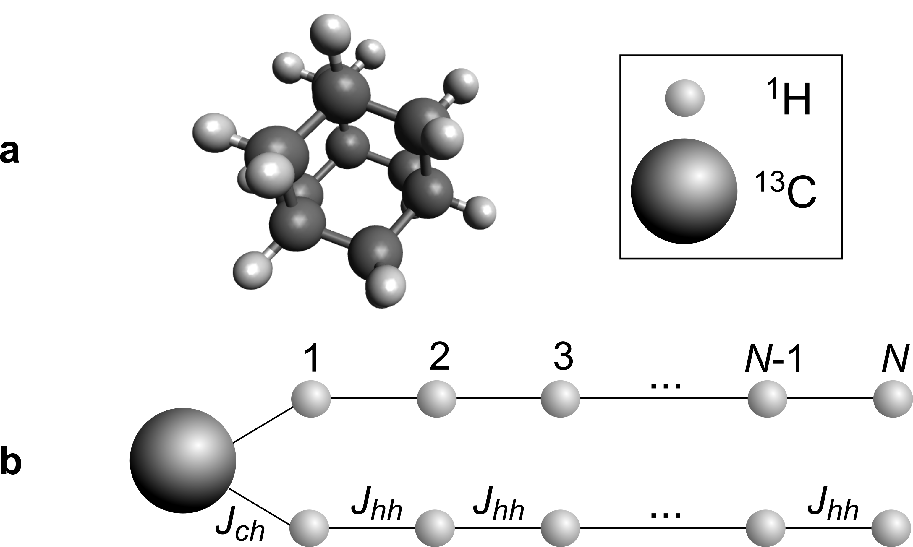
Figure 1: Spin system: a Adamantane molecule and b representation of our spin system model composed by a${}^{13}C$ atom coupled to two linear chains of $N$ ${}^{1}H$ atoms each.

$${\displaystyle H_{SE}}= J_{ch}\sum_{\alpha=a,b}S_{z}I_{z}^{\alpha,1},$$ (1)

$$H_{E}= J_{hh}\sum_{\alpha=a,b}\sum_{k=1}^{N-1}\left[2I_{z}^{\alpha,k}I_{z}^{\alpha,k+1}-\left(I_{x}^{\alpha,k}I_{x}^{\alpha,k+1}+I_{y}^{\alpha,k}I_{y}^{\alpha,k+1}\right)\right],$$ (2)

where the index $\alpha=a,b$ represents the arrays of hydrogen spins, being the first one of each array coupled directly to the ${}^{13}C$. The index $k$ represents the $k^{th}$ ${}^{1}H$ of the bath, being $2N$ the total number of ${}^{1}H$ nuclear spins in the bath system ($N$ in each array). $J_{ch}$ and $J_{hh}$ are, respectively, the carbon-hydrogen and hydrogen-hydrogen coupling constants.

The natural interaction between the carbon and the hydrogen is not able to promote flips on the qubit system (carbon spin), thus not being immediately useful for our proposal. To engineer the desired reservoir we firstly need to build up interactions that allow the exchange of energy between the system and the environment. To this end, we need to manipulate the nuclear spins in order to obtain an effective suitable Hamiltonian. This can be done by applying the sequence of radiofrequency (r.f.) pulses, being each one followed by a free evolution governed by the system Hamiltonian $H$ during a short time interval $\Delta t$. This sequence is then described by the evolution operator

$$U(\tau_{c})=e^{-\frac{i}{2\hbar}H\Delta t}P_{4}e^{-\frac{i}{\hbar}H\Delta t}P_{3}e^{-\frac{i}{\hbar}H\Delta t}P_{2}e^{-\frac{i}{\hbar}H\Delta t}P_{1}e^{-\frac{i}{2\hbar}H\Delta t},$$ (3)

where $P_{1}=exp\left[-i\frac{\pi}{2}\left(S_{x}+I_{x}\right)\right]$, $P_{2}=exp\left[i\frac{\pi}{2}\left(S_{x}+I_{x}\right)\right]$, $P_{3}=exp\left[-i\frac{\pi}{2}\left(S_{y}+I_{y}\right)\right]$, and $P_{4}=exp\left[i\frac{\pi}{2}\left(S_{y}+I_{y}\right)\right]$ are r.f. pulse operators that make the spins $I$ and $S$ to flip at angles $\nicefrac{{\pi}}{{2}}$ in the $x$, $-x$, $y$ and $-y$ directions, respectively.

We can rewrite the equation (3) as a single evolution operator governed by an effective Hamiltonian, i.e., $U(t)=e^{-\frac{i}{\hbar}H_{eff}t}$, which can be calculated using average Hamiltonian theory (SlichterLivro1990, ):

$$H_{eff}=\bar{H}_{0}+\bar{H}_{1}+\bar{H}_{2}+...\bar{H}_{p}.$$ (4)

The terms of $H_{eff}$ can be calculated from the Magnus’ expansion (Magnus1954, ), where $\bar{H}_{0}$ is the first approximation for the Hamiltonian and $\bar{H}_{1}\text{, }\bar{H}_{2},...,\bar{H}_{p}$ are the correction terms (Maricq1982, ). The time interval between the different pulses used in this work is designed to be small enough such that the correction terms are reduced close to zero, remaining only the zeroth-order term $\bar{H}_{0}$, which is given by (SlichterLivro1990, )

$$\bar{H}_{0}=\frac{1}{t}\sum_{j=1}^{M}\Delta t_{j}\tilde{H}_{j},$$ (5)

where $\tilde{H}_{j}=T_{j}^{\dagger}HT_{j}$, ${\displaystyle T_{j}=\prod_{m=1}^{M}P_{m}}$, and $t={\displaystyle\sum_{j=1}^{M}}\Delta t_{j}$, being $M$ the number of r.f. pulses. $\Delta t_{j}$ is the time duration that the system evolves under the $\tilde{H}_{j}$ Hamiltonian. As a result, considering our linear spin chain model described by the Hamiltonian $H$ (2), we derive the effective Hamiltonian for the carbon-hydrogen and hydrogen-hydrogen interactions:

$${\displaystyle H_{eff}^{SE}=} J_{ch}^{eff}\sum_{\alpha=a,b}\left(2S_{z}I_{z}^{\alpha,1}+S_{x}I_{x}^{\alpha,1}+S_{y}I_{y}^{\alpha,1}\right),$$ (6)

$$H_{eff}^{E}= J_{hh}^{eff}\sum_{\alpha=a,b}\sum_{k=1}^{N-1}\left[2I_{z}^{\alpha,k}I_{z}^{\alpha,k+1}-\left(I_{x}^{\alpha,k}I_{x}^{\alpha,k+1}+I_{y}^{\alpha,k}I_{y}^{\alpha,k+1}\right)\right].$$ (7)

$J_{ch}^{eff}=J_{ch}/4\text{ and }J_{hh}^{eff}=J_{hh}/4$ are, respectively, the effective coupling constants of the interactions between the nuclear spin of the ${}^{13}C$ and its first neighboring hydrogens and between the nuclear hydrogen spins of each chain obtained after the application of the pulse sequence described in equation (3). In Figure 2 we plot the magnetization of the carbon spin in $z$ direction ($M_{z}=\left\langle S_{z}\right\rangle$) as a function of time, derived by solving numerically the Schrödinger equation, either using the effective Hamiltonian (dashed line), Eqs. (6) and (7), or by simulating the propagator (3) (full, dotted and dashed-dotted lines). We considered the initial state of the system as $|1\rangle$ (excited) for the carbon nuclear spin and $|0\rangle$ (ground) for all hydrogen nuclear spins. The time duration of each pulse was fixed as $\tau_{p}=9.89$ $\mu s$ in all cases. However, we considered different time intervals between each pulse: $\Delta t=15.10$ $\mu s$, $1.22$ $\mu s$ and $0.10$ $\mu s$, for a sequence of $100$, $225$ and $250$ cycles during the total time evolution of $10$ $ms$. We can observe that the lower the value of $\Delta t$, the better the match between the results predicted via $H_{eff}$ and those obtained from the pulse sequence described by equation 3.

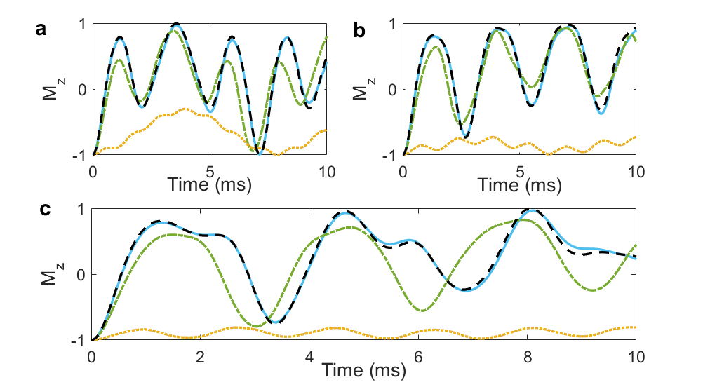
Figure 2: Time evolution of the $z$ component of the magnetization of the carbon nuclear spin ($M_{z}$) coupled to two symmetric chains containing a total of a 6, b 8 and c 10 spins of hydrogen. The dashed black line was derived using $H_{eff}$ while the yellow (dotted), green (dashed-dotted) and blue (full) lines refer to the simulations of $100$ ($\Delta t=15.10$ $\mu s$), 225 ($\Delta t=1.228$ $\mu s$) and 250 ($\Delta t=0.10$ $\mu s$) cycles, respectively, with pulse sequence described by equation 3. The parameters used are: $\tau_{p}=9.89$ $\mu s$, $J_{ch}^{eff}=550$ rad $s^{-1}$, $J_{hh}^{eff}=980$ rad $s^{-1}$. The initial state is $|1\rangle$ for the carbon nuclear spin and $|0\rangle$ for all hydrogen spins.

The control of the spin temperature is done by adjusting the hydrogen nuclear spin state (Purcell1951, ; Quan2007, ; Carr2013, ). For example, by inverting the population of the hydrogen spins, the environment can be treated as having effective negative temperatures (Struchtrup2018, ). To study the dynamics and thermalization of the carbon spin system we consider different sizes of the environment, for different initial states. Fig. 3a shows how the dynamics of our carbon spin system behaves when we increase the size of the environment (number of hydrogen spins) when the carbon spin system is prepared in the excited state $|1\rangle$ and the environment spins with positive temperature, i.e., all of them in the ground state $|0\rangle$. The coupling strengths $J_{ch}^{eff}=550$ rad $s^{-1}$and $J_{hh}^{eff}=980$ rad $s^{-1}$ were calibrated from the experimental data shown in Fig. 4. We observe that the greater the number of hydrogens in the spin system, the better the thermalization. In Fig. 3b we also plot the degree of entanglement between the carbon and the first hydrogen spin (first array), quantified by the Entanglement of Formation ($EoF$) (Wootters1998, ). A general bipartite system is entangled if the global density matrix of the composite system $\rho$ can not be written as as separable state, i.e., if $\rho\neq\sum_{i}P_{i}\rho_{C}^{(i)}\otimes\rho_{H}^{(i)}$, being $\rho_{C}^{(i)}$ ($\rho_{H}^{(i)}$) any possible reduced density matrix for the carbon (hydrogen) nuclear spin. When a system is in a separable (not entangled) state $EoF=0$, while $EoF=1$ for maximally entangled states. From Fig. 3b we see that, for chains of few hydrogen spins, the entanglement between carbon and the first hydrogen spin oscillates all the time. But, as we increase the number of hydrogen spins, the carbon spin initially gets highly entangled with the first hydrogen spin, and then the degree of entanglement decreases, becoming close to zero. This means that entanglement moves to the other hydrogen spins, disentangling the carbon spin from the hydrogen chains. At the same time, the state of the carbon spin approaches the initial hydrogen spin state. This is a clear signature that the hydrogen spin chains work out as a real thermal bath for the carbon spin, as desired.

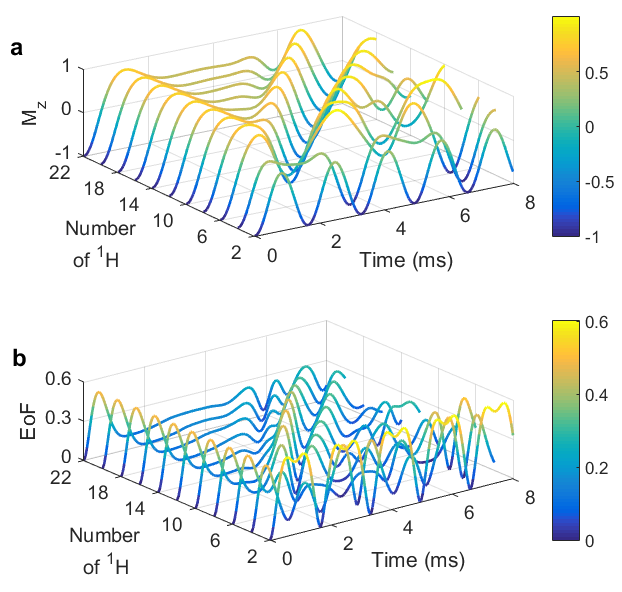
Figure 3: a $z$ component of the magnetization of the carbon nuclear spin as a function of time and number of qubits of the bath, derived via solution of the Schrödinger equation with $H_{eff}$ and b $EoF$ between the carbon and first hydrogen spin (first array). The parameters used are: $\tau_{p}=9.89$ $\mu s$, $\Delta t=0.10$ $\mu s$, $J_{ch}^{eff}=550$ rad $s^{-1}$ and $J_{hh}^{eff}=980$ rad $s^{-1}$. The initial state is $|1\rangle$ for the carbon nuclear spin and $|0\rangle$ for all hydrogen spins.

Experimental results: We prepared different initial states for ${}^{13}C$ and ${}^{1}H$ simulating different temperatures of the spin bath for the main qubit (carbon spin) and measured the expected value of $z$ component of magnetization. Initially we start from the thermal equilibrium at room temperature. In this high-temperature limit, the spin states are almost equally populated with the excess of the lower energy state on the order of $10^{-5}$. Firstly the excess population of the carbon spins is prepared in the excited state $|1\rangle$ and the hydrogen spins are kept in the thermal equilibrium state (with excess of population in the ground state $|0\rangle$), Figure 4a. Then we prepared the excess population of carbon spins in the state $|0\rangle$ and the hydrogen spins in the thermal equilibrium with negative temperature (with excess of population in the state $|1\rangle$), Figures 4b. This is obtained by inverting the population of all hydrogen spins with r.f. pulses. During a short period of time, compared to the thermal relaxation time of the sample, the transitions between the magnetic energy levels can be neglected, keeping the hydrogen spins in an state corresponding to the negative room temperature thermal state. By modulating the system-environment interaction, i.e., the carbon-hydrogen interaction, with the sequence of r.f. pulses it is possible to promote energy exchange between the system and the environment. The resulting situation is equivalent to put the carbon spins in contact to a thermal bath with negative temperature. Still in Figure 4, we do the same for the bath at infinite temperature, i.e. the hydrogen spins of the bath is prepared in the mixed state without population excess $\rho=\frac{1}{2}\left(|0\rangle\langle 0|+|1\rangle\langle 1|\right)$, Figures 4c and 4d. In all cases we can observe, in very good agreement between the experimental and the prediction of our model, that the qubit system tends to thermalize in the state of the qubit bath, and this happens even when the qubit system is in the ground state and the qubits bath are in the excited state.

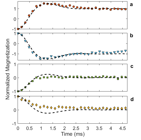
Figure 4: Normalized $z$ component of the magnetization of the carbon nuclear spin ($M_{z}$) as a function of time for the initial states: a Carbon in $|1\rangle$ and hydrogens in $|0\rangle$; b Carbon in $|0\rangle$ and hydrogens in $|1\rangle$; Hydrogens in $\rho=\frac{1}{2}\left(|0\rangle\langle 0|+|1\rangle\langle 1|\right)$ and carbon in c $|1\rangle$ and d $|0\rangle$. The symbols refer to experimental data while the dashed lines are derived theoretically via $H_{eff}$ (with $N=22$ hydrogen spins). The parameters used here are $J_{ch}^{eff}=550$ rad $s^{-1}$and $J_{hh}^{eff}=980$ rad $s^{-1}$.

Slight difference between experimental and theoretical data can be observed in different regions in all panels of Figure 4. The origin of these errors are mainly due to r.f. pulse imperfections and the natural relaxation of the spins. In NMR, the thermal relaxation time is associated to the spin-lattice relaxation, which occurs at a characteristic times $T_{1}$, which for our system are $T_{1}^{H}=0.9$ $s$ and $T_{1}^{C}=1.6$ $s$. These source of errors may reduce the fidelity $\mathscr{F}$ (Wang2008, ), which is a parameter commonly used to quantify the performance of quantum operations by checking the compatibility between experimental and theoretical operators. We can map a process matrix into a set of transformations of unitary evolutions from the initial and final density matrices (Chuang1997, ). For this purpose we use the equation $\rho_{f}={\displaystyle\sum_{mn}}\chi_{mn}E_{m}\rho_{i}E_{n}^{\dagger}$, where $\rho_{i}$ and $\rho_{f}$ are the density matrices at the beginning and end of the process, and the operators $E_{m}=I,S_{x},iS_{y},S_{z}$ must form a basis. Thus the propagator $\chi_{mn}$ for the process can therefore be quantified.

We performed a quantum tomography process to obtain the implemented propagator and use $\mathscr{F}$ to compare the theoretical and experimental results for $\chi_{mn}$. The fidelity $\mathscr{F}$ between the experimental and ideal matrices of the thermalization process at positive temperature, Figures 5a and 5b, and of the thermalization process at negative temperature, Figures 5c and 5d, are 0.999 and 0.984, respectively.

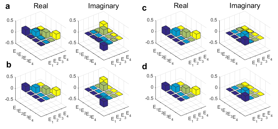
Figure 5: Theoretical and experimental process matrices of $\chi_{mn}$ of the thermalization processes of the Figures 4a and 4b. The Figures in the left (right) are the real (imaginary) part. a and b are, respectively, the experimental and theoretical process matrices of the Fig. 4a. Panels c and d are, respectively, the experimental and theoretical process matrices of the 4b.

Quantum thermal machine of a single reservoir: As an application for this reservoir technique here implemented, we propose a single reservoir quantum thermal machine at an effective negative temperature. The spin 1/2 of the ${}^{13}C$ nucleus is the working medium, and the ensemble of spin 1/2 of ${}^{1}H$ nuclei plays the role of the hot thermal reservoir. The Quantum thermal machine can be described by the relation

$$\rho_{ground}\overset{thermalization}{\rightarrow}\rho_{1}\overset{U(\tau)}{\rightarrow}\rho_{2}\overset{thermalization}{\rightarrow}\rho_{1}.$$ (8)

Firstly the qubit system (carbon nucleus) is put in contact with the hot reservoir, to absorb heat from it (step described in Fig. 4b, i.e., step $\rho_{ground}\rightarrow\rho_{1}$ in relation (8)). Therefore, the ${}^{13}C$ spin will initially be in a thermal state equivalent to $\rho_{1}=e^{-\beta_{1}H_{1}}/Z_{1}$, where $H_{1}=-\frac{1}{2}\hbar\omega_{1}S_{z}$ is Zeeman Hamiltonian, being $\hbar$ the Planck’s constant, $\omega_{1}$ the Larmor frequency of the ${}^{13}C$ nuclear spin, $Z_{1}$ the partition function, and $\beta_{1}=1/k_{B}T$ such that $T<0$ is the spin temperature and $k_{B}$ is the Boltzmann constant. Then, our thermodynamic cycle consists of two steps. (i) In the first step an unitary evolution operator $U(\tau)$ is applied to bring the ${}^{13}C$ spin state to $\rho_{2}=U(\tau)\rho_{1}U^{\dagger}(\tau)$ (step $\rho_{1}\rightarrow\rho_{2}$ in relation (8)). The Hamiltonian $H_{1}$ changes in this process, which is the one where we can extract work from the machine, then turning to its initial form at the end of this step. (ii) The second step consists of thermalization with the hot thermal reservoir (step $\rho_{2}\rightarrow\rho_{1}$ in relation (8)), when the qubit absorbs heat and then goes back to the state $\rho_{1}$. Here the Hamiltonian $H_{1}$ remains unchanged.

In Figure 6 we show the application of four different unitary operators: Fig. 6a $U_{x}=exp\left(-i\frac{\pi}{2}S_{x}\right)$, Fig. 6b $U_{y}=exp\left(-i\frac{\pi}{2}S_{y}\right)$, Fig. 6c $U_{\pi}=exp\left(-i\pi S_{x}\right)$, and Fig. 6d $U_{I}=exp\left(-2i\pi S_{y}\right)=\mathbb{I}$, where $U_{x}$ and $U_{y}$ are operators that represent pulses in the $x$ and $y$ directions, allowing the ${}^{13}C$ spin to flip by an angle of $\nicefrac{{\pi}}{{2}}$. $U_{\pi}$ is the operator which rotates the spin by an angle of $\pi$ and $U_{I}$ is an identity operator (a complete rotation around the Bloch sphere). The total magnetization in the $x$, $y$ and $z$ directions - $M_{U}=(M_{x},M_{y},M_{z})$ - immediately after each unitary operation (second point in Fig. 6) is $M_{U_{x}}=(0.11,-0.92,0.20)\mathrm{a.u.}$, $M_{U_{y}}=(0.96,-0.05,0.13)\mathrm{a.u.}$, $M_{U_{\pi}}=(-0.01,-0.01,1.0)\mathrm{a.u.}$, and $M_{U_{I}}=(-0.01,0.15,-0.87)\mathrm{a.u.}$.

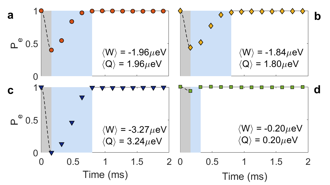
Figure 6: Population ($\mathrm{P_{e}}$) of the excited state as a function of time for different unitary operations. We consider the beginning of our cycle in $t=0$, starting from a thermalized state with the environment at a negative effective temperature. The unitary operations performed were: a $U_{x}=exp\left(-i\frac{\pi}{2}S_{x}\right)$, b $U_{y}=exp\left(-i\frac{\pi}{2}S_{y}\right)$, c $U_{\pi}=exp\left(-i\pi S_{x}\right)$ and d $U_{I}=exp\left(-2i\pi S_{x}\right)$. The work is calculated in the unitary operation region (gray region) and the heat exchanged with the hot thermal reservoir is calculated in the thermalization region with the reservoir (blue region).

The gray region in Fig. 8 refers to the carbon nucleus leaving the thermalized state with the hot reservoir (spin bath) $\rho_{1}$ and going to the state $\rho_{2}$ as a result of the unitary operation. The average work $\left\langle W\right\rangle$ performed by the quantum thermal machine is then given by (see SM of (deAssis2019, ))

$$\left\langle W\right\rangle=Tr\left[\rho_{2}H_{1}\right]-Tr\left[\rho_{1}H_{1}\right]=-\hbar\omega_{1}\xi\tanh\left({\textstyle\frac{1}{2}}\left|\beta_{1}\right|\hbar\omega_{1}\right),$$ (9)

where $\xi=\left|\langle 1|U(t)|0\rangle\right|^{2}\geq 0$ is the transition probability between initial state $|0\rangle$ and $|1\rangle$ and $\beta_{1}=-\left|\beta_{1}\right|<0$. Here $\left\langle W\right\rangle<0$ means that the work is done by the machine. The blue region in Fig. 6 refers to the thermalization process with the hot reservoir, immediately after the carbon spin being in the state $\rho_{2}$, which brings it back to the state $\rho_{1}.$ The average heat $\left\langle Q\right\rangle$ exchanged with the hot thermal reservoir is then (see SM of (deAssis2019, ))

$$\left\langle Q\right\rangle=Tr\left[\rho_{1}H_{1}\right]-Tr\left[\rho_{2}H_{1}\right]=\hbar\omega_{1}\xi\tanh\left({\textstyle\frac{1}{2}}\left|\beta_{1}\right|\hbar\omega_{1}\right).$$ (10)

The results obtained experimentally for the different unitary operations are: $\left\langle W\right\rangle_{U_{x}}=-\left(1.97\pm 0.28\right)\mu eV$, $\left\langle W\right\rangle_{U_{y}}=-\left(1.84\pm 0.21\right)\mu eV$, $\left\langle W\right\rangle_{U_{\pi}}=-\left(3.27\pm 0.22\right)\mu eV$, and $\left\langle W\right\rangle_{U_{I}}=-\left(0.20\pm 0.21\right)\mu eV$. The heat absorbed from the reservoir are: $\left\langle Q\right\rangle_{U_{x}}=\left(1.96\pm 0.29\right)\mu eV$, $\left\langle Q\right\rangle_{U_{y}}=\left(1.79\pm 0.18\right)\mu eV$, $\left\langle Q\right\rangle_{U_{\pi}}=\left(3.24\pm 0.22\right)\mu eV$, and $\left\langle Q\right\rangle_{U_{I}}=\left(0.20\pm 0.21\right)\mu eV$. Thus, the efficiency $\eta=\left|\frac{\left\langle W\right\rangle}{\left\langle Q\right\rangle}\right|$ for each process is $\eta_{U_{x}}=1.00\pm 0.05$, $\eta_{U_{y}}=1.03\pm 0.06$, $\eta_{U_{\pi}}=1.01\pm 0.02$ and $\eta{}_{U_{I}}=1.00\pm 0.12$, i.e., whenever the final state is different from the initial one, the machine absorbs heat and converts it entirely into liquid work.

To conclude, here we have applied the reservoir engineering technique to build up reservoirs with arbitrary temperatures, even effective negative ones, for qubit systems. Our system is composed by a nuclear carbon spin (the main qubit) coupled to a large number of nuclear hydrogen spins. By properly manipulating the initial hydrogen state and the carbon-hydrogen and hydrogen-hydrogen nuclear spin interactions, the effective dynamics describes the interaction of a qubit with reservoirs at arbitrary temperatures. We have shown theoretically that, the larger the number of hydrogen spins, the better the hydrogen arrays work out as a bath for the main qubit, which is in excellent agreement with our experimental results. As an application, we have implemented a single reservoir heat engine. Several papers have discussed how to increase the efficiency of quantum thermal machines, for example via the use of quantum coherence (Scully2003, ; Serra2019a, ) or artificial environments as squeezed reservoirs (Myatt2000, ; Murch2013, ). However, as shown in our work, the simple use of a single reservoir with negative effective temperature allows us to obtain maximum efficiency ($\eta$ = 1) regardless of the unitary transformation performed on the qubit (making sure that the final state is different from the initial one), thus being, to the best of our knowledge, the simpler and most efficient quantum thermal machine implemented so far. Naturally, to achieve this result we need to build up this artificial reservoir, with inverted population, which demands energy, but this is the price we have to pay for this new technology. For instance, this is quite similar to what happens to laser, another system based on inverted population, which is responsible for great scientific and technological advances in the last decades. Thus, we believe our single reservoir heat engine can be another interesting application for inverted population systems and that the results presented here can be very useful for investigating fundamental and applications of quantum thermodynamics in general, for instance, to study quantum thermal engines which require specific kinds of reservoirs (Klaers2017, ; deAssis2019, ; deAssis2019b, ).

- [1] J. Gemmer, M. Michel, and G. Mahler. Quantum Thermodynamics. Springer Verlag, Berlin, 2004.
- [2] R. Alicki. The quantum open system as a model of the heat engine. Journal of Physics A: Mathematical and General, 12(5):L103–L107, may 1979.
- [3] H. T. Quan, Yu-xi Liu, C. P. Sun, and Franco Nori. Quantum thermodynamic cycles and quantum heat engines. Phys. Rev. E, 76:031105, Sep 2007.
- [4] E. M. Purcell and R. V. Pound. A nuclear spin system at negative temperature. Phys. Rev., 81:279–280, Jan 1951.
- [5] N. F. Ramsey. Thermodynamics and statistical mechanics at negative absolute temperatures. Phys. Rev., 103:20–28, Jul 1956.
- [6] L. D. Carr. Negative temperatures? Science, 339(6115):42–43, 2013.
- [7] S. Braun, J. P. Ronzheimer, M. Schreiber, S. S. Hodgman, T. Rom, I. Bloch, and U. Schneider. Negative absolute temperature for motional degrees of freedom. Science, 339(6115):52–55, 2013.
- [8] R. J. de Assis, T. M. de Mendonça, C. J. Villas-Boas, A. M. de Souza, R. S. Sarthour, I. S. Oliveira, and N. G. de Almeida. Efficiency of a quantum otto heat engine operating under a reservoir at effective negative temperatures. Phys. Rev. Lett., 122:240602, Jun 2019.
- [9] J. F. Poyatos, J. I. Cirac, and P. Zoller. Quantum reservoir engineering with laser cooled trapped ions. Phys. Rev. Lett., 77:4728–4731, Dec 1996.
- [10] C. J. Myatt, B. E. King, Q. A. Turchette, C. A. Sackett, D. Kielpinski, W. M. Itano, C. Monroe, and D. J. Wineland. Decoherence of quantum superpositions through coupling to engineered reservoirs. Nature, 403:269–273, Jan 2000.
- [11] K. W. Murch, S. J. Weber, K. M. Beck, E. Ginossar, and I. Siddiqi. Reduction of the radiative decay of atomic coherence in squeezed vacuum. Nature, 499:62–65, Jul 2013.
- [12] A. R. R. Carvalho, P. Milman, R. L. de Matos Filho, and L. Davidovich. Decoherence, pointer engineering, and quantum state protection. Phys. Rev. Lett., 86:4988–4991, May 2001.
- [13] T. Werlang, R. Guzmán, F. O. Prado, and C. J. Villas-Bôas. Generation of decoherence-free displaced squeezed states of radiation fields and a squeezed reservoir for atoms in cavity qed. Phys. Rev. A, 78:033820, Sep 2008.
- [14] S. Pielawa, G. Morigi, D. Vitali, and L. Davidovich. Generation of einstein-podolsky-rosen-entangled radiation through an atomic reservoir. Phys. Rev. Lett., 98:240401, Jun 2007.
- [15] T. Werlang and C. J. Villas-Boas. Theoretical method for the generation of a dark two-mode squeezed state of a trapped ion. Phys. Rev. A, 77:065801, Jun 2008.
- [16] F. O. Prado, E. I. Duzzioni, M. H. Y. Moussa, N. G. de Almeida, and C. J. Villas-Bôas. Nonadiabatic coherent evolution of two-level systems under spontaneous decay. Phys. Rev. Lett., 102:073008, Feb 2009.
- [17] F. Verstraete, M.l M. Wolf, and J. Ignacio Cirac. Quantum computation and quantum-state engineering driven by dissipation. Nature Physics, 5:633–636, Jul 2009.
- [18] Yusuke Hama, William J. Munro, and Kae Nemoto. Relaxation to negative temperatures in double domain systems. Phys. Rev. Lett., 120:060403, Feb 2018.
- [19] Gonzalo A. Álvarez and Dieter Suter. Measuring the spectrum of colored noise by dynamical decoupling. Phys. Rev. Lett., 107:230501, Nov 2011.
- [20] Marko Lovrić, Hans Georg Krojanski, and Dieter Suter. Decoherence in large quantum registers under variable interaction with the environment. Phys. Rev. A, 75:042305, Apr 2007.
- [21] G. A. Alvarez, A. Ajoy, X. Peng, and D. Suter. Performance comparison of dynamical decoupling sequences for a qubit in a rapidly fluctuating spin bath. Phys. Rev. A, 82:042306, Oct 2010.
- [22] A. Ajoy, G. A. Alvarez, and D. Suter. Optimal pulse spacing for dynamical decoupling in the presence of a purely dephasing spin bath. Phys. Rev. A, 83:032303, Mar 2011.
- [23] A. M. Souza, G.A. Alvarez, and D. Suter. Robust dynamical decoupling for quantum computing and quantum memory. Phys. Rev. Lett., 106:240501, 2011.
- [24] A. Abragam. Principles of magnetism. Oxford University Press, Oxford, 1962.
- [25] C. P. Slichter. Principles of magnetic resonance, volume 3. Springer, Berlin, 1990.
- [26] W. Magnus. On the exponential solution of differential equations for a linear operator. Communications on Pure and Applied Mathematics, 7(4):649–673, 1954.
- [27] M. M. Maricq. Application of average hamiltonian theory to the nmr of solids. Phys. Rev. B, 25:6622–6632, Jun 1982.
- [28] H. Struchtrup. Work storage in states of apparent negative thermodynamic temperature. Phys. Rev. Lett., 120:250602, Jun 2018.
- [29] W. K. Wootters. Entanglement of formation of an arbitrary state of two qubits. Phys. Rev. Lett., 80:2245–2248, Mar 1998.
- [30] X. Wang, C.-S. Yu, and X.X. Yi. An alternative quantum fidelity for mixed states of qudits. Physics Letters A, 373(1):58 – 60, 2008.
- [31] I. L. Chuang and M. A. Nielsen. Prescription for experimental determination of the dynamics of a quantum black box. Journal of Modern Optics, 44(11-12):2455–2467, 1997.
- [32] Marlan O. Scully, M. Suhail Zubairy, Girish S. Agarwal, and Herbert Walther. Extracting work from a single heat bath via vanishing quantum coherence. Science, 299(5608):862–864, 2003.
- [33] Patrice A. Camati, Jonas F. G. Santos, and Roberto M. Serra. Coherence effects in the performance of the quantum otto heat engine. Phys. Rev. A, 99:062103, Jun 2019.
- [34] J. Klaers, S. Faelt, A. Imamoglu, and E. Togan. Squeezed thermal reservoirs as a resource for a nanomechanical engine beyond the carnot limit. Phys. Rev. X, 7:031044, Sep 2017.
- [35] R. J. de Assis, C. J. Villas-Boas, and N. G. de Almeida. Feasible platform to study negative temperatures. 52(6):065501, feb 2019.