Simultaneous State and Unknown Input Set-Valued Observers for Some Classes of Nonlinear Dynamical Systems

Abstract

In this paper, we propose fixed-order set-valued (in the form of $\ell_{2}$-norm hyperballs) observers for some classes of nonlinear bounded-error dynamical systems with unknown input signals that simultaneously find bounded hyperballs of states and unknown inputs that include the true states and inputs. Necessary and sufficient conditions in the form of Linear Matrix Inequalities (LMIs) for the stability (in the sense of quadratic stability) of the proposed observers are derived for ($\mathcal{M},\gamma$)-Quadratically Constrained (($\mathcal{M},\gamma$)-QC) systems, which includes several classes of nonlinear systems: (I) Lipschitz continuous, (II) ($\mathcal{A},\gamma$)-QC* and (III) Linear Parameter-Varying (LPV) systems. This new quadratic constraint property is at least as general as the incremental quadratic constraint property for nonlinear systems and is proven in the paper to embody a broad range of nonlinearities. In addition, we design the optimal $\mathcal{H}_{\infty}$ observer among those that satisfy the quadratic stability conditions and show that the design results in Uniformly Bounded-Input Bounded-State (UBIBS) estimate radii/error dynamics and uniformly bounded sequences of the estimate radii. Furthermore, we provide closed-form upper bound sequences for the estimate radii and sufficient condition for their convergence to steady state. Finally, the effectiveness of the proposed set-valued observers is demonstrated through illustrative examples, where we compare the performance of our observers with some existing observers.

,

1 Introduction

1.1 Motivation

Cyber-physical systems (CPS), e.g., power grids, autonomous vehicles, medical devices, etc., are systems in which computational and communication components are deeply intertwined and interacting with each other in several ways to control physical entities. Such safety-critical systems, if jeopardized or malfunctioning, can cause serious detriment to their operators, controlled physical components and the people utilizing them. A need for CPS security and for new designs of resilient estimation and control has been accentuated by recent incidents of attacks on CPS, e.g., the Iranian nuclear plant, the Ukrainian power grid and the Maroochy water service [6, 14, 40, 44, 55]. Specifically, false data injection attack is one of the most serious types of attacks on CPS, where malicious and/or strategic attackers inject counterfeit data signals into the sensor measurements and actuator signals to cause damage, steal energy etc. Given the strategic nature of these false data injection signals, they are not well-modeled by a zero-mean, Gaussian white noise nor by signals with known bounds. Nevertheless, reliable estimates of states and unknown inputs are indispensable and useful for the sake of attack identification, resilient control, etc. Similar state and input estimation problems can be found across a wide range of disciplines, from input estimation in physiological systems [13], to fault detection and diagnosis [36], to the estimation of mean areal precipitation [28].

1.2 Literature Review

Much of the research focus has been on simultaneous input and state estimation for stochastic systems with unknown inputs, assuming that the noise signals are Gaussian and white, via minimum variance unbiased (MVU) estimation approaches (e.g., [17, 18, 51, 53]), modified double-model adaptive estimation methods (e.g, [30]), or robust regularized least square approaches as in [1]. However, in order to address “set-membership” estimation problems in bounded-error settings, as is considered in this paper, where set-valued uncertainties are considered and sets of states and unknown inputs that are compatible with measurements are desired (cf. [49] for a comprehensive discussion), the development of set-theoretic approaches are needed.

In the context of attack-resilient estimation, numerous approaches were proposed for deterministic systems (e.g., [12, 15, 35, 42]), stochastic systems (e.g., [27, 52, 54]) and bounded-error systems [32, 34, 50], against false data injection attacks. However, these approaches mainly yield point estimates, i.e, the most likely or best single estimate, as opposed to set-valued estimates. On the other hand, the work in [34] only computes error bounds for the initial state and [32] assumes zero initial states and does not consider any optimality criteria.

In addition, unknown input observer designs for different classes of discrete-time nonlinear systems are relatively scarce. The method proposed in [45] leverages discrete-time sliding mode observers for calculating state and unknown input point estimates, assuming that the unknown inputs have known bounds and evolve as known functions of states, which may not be directly applicable when considering adversaries in the system. The authors in [29] proposed an LMI-based state estimation approach for globally Lipschitz nonlinear discrete-time systems, but did not consider unknown input reconstruction. An LMI-based approach was also used in [19] for simultaneous estimation of state and unknown input for a class of continuous-time dynamic systems with Lipschitz nonlinearities, but the authors did not address optimality nor stability properties for their observer, as well as only considered point estimates.

The work in [3] designed an asymptotic observer to calculate point estimates for a class of continuous-time systems whose nonlinear terms satisfy an incremental quadratic inequality property. Similar work was done for the same class of discrete-time nonlinear systems in [8], while the set-valued state estimation approach in [39] uses mean value and first-order Taylor extensions to efficiently propagate constrained zonotopes through nonlinear mappings. However, none of them addressed unknown input estimation. Moreover, the restrictive assumption of bounded unknown inputs is needed in order to obtain convergent estimates.

Considering bounded unknown inputs, but with unknown bounds, the work in [10] applied second-order series expansions to construct observer for state estimation in nonlinear discrete-time systems. The authors also provided sufficient conditions for stability and optimality of the designed estimator. However, their method does not compute unknown input estimates. On the other hand, in a recent and interesting work in [7], the authors designed an observer for reconstruction of unknown exogenous inputs in nonlinear continuous-time systems with unknown and potentially unbounded inputs, providing sufficient LMI conditions for $\mathcal{L}_{\infty}$-stability of the observer. However, their observer does not simultaneously estimate the state, the unknown input estimates are point estimates and the optimality of their approach was not analyzed.

The author in [49] and references therein discussed the advantages of set-valued observers (when compared to point estimators) in terms of providing hard accuracy bounds, which are important to guarantee safety [5]. In addition, the use of fixed-order set-valued methods can help decrease the complexity of optimal observers [31], which grows with time. Hence, a fixed-order set-valued observer for linear time-invariant discrete time systems with bounded errors, was presented in [49], that simultaneously finds bounded hyperballs of compatible states and unknown inputs that are optimal in the minimum $\mathcal{H}_{\infty}$-norm sense, i.e., with minimum average power amplification. In our preliminary work [22], we extended the approach in [49] to linear parameter-varying systems, while in [23], we generalized the method to switched linear systems with unknown modes and sparse unknown inputs (attacks), and in [24, 25] we considered simultaneous input and state interval-valued observers. In this paper, we aim to further design novel set-valued observers for broader classes of nonlinear systems.

1.3 Contribution

The goal of this paper is to bridge the gap between set-valued state estimation without unknown inputs and point-valued state and unknown input estimation for a broad range of time-varying nonlinear dynamical systems, with nonlinear observation functions. In particular, we propose fixed-order set-valued (in the form of $\ell_{2}$-norm hyperball s) observers for nonlinear discrete-time bounded-error systems that simultaneously find uniformly bounded sets of states and unknown inputs that contain the true state and unknown input, are compatible/consistent with measurement outputs as well as nonlinear observation function, and are optimal in the minimum $\mathcal{H}_{\infty}$-norm sense, i.e., with minimum average power amplification.

First, we introduce a novel class of time-varying nonlinear vector fields that we call $(\mathcal{M},\gamma)$-Quadratically Constrained ($(\mathcal{M},\gamma)$-QC) functions and show that they include a broad range of nonlinearities. We also derive some results on the relationship between $(\mathcal{M},\gamma)$-QC functions with other classes of nonlinearities, such as the incrementally quadratically constrained, Lipschitz continuous and linear parameter-varying (LPV) functions.

Then, we present our three-step recursive set-valued observer for nonlinear discrete-time systems. In particular, in the absence of noise, we derive sufficient and necessary conditions in the form of LMIs for the existence and stability of the observer in the sense of quadratic stability for this class of $(\mathcal{M},\gamma)$-QC functions, as well as three classes of nonlinearities: (I) Lipschitz continuous, (II) ($\mathcal{A},\gamma$)-QC* and (III) LPV systems.

Furthermore, we design $\mathcal{H}_{\infty}$ observers among those that satisfy the quadratic stability conditions, using semi-definite programs with additional LMIs constraints for each of the aforementioned system classes. Then, we show that our $\mathcal{H}_{\infty}$ observer design leads to estimate radii dynamics that are Uniformly Bounded-Input Bounded-State (UBIBS), which equivalently results in uniformly bounded sequences of the estimate radii in the presence of noise. Moreover, we derive closed-form expressions for upper bound sequences for the estimate radii as well as sufficient conditions for the convergence of these radii upper bound sequences to steady state.

Note that we consider completely unknown inputs (different from noise signals) without imposing any assumptions on them (such as being norm bounded, with limited energy or being included in some known set). Considering resilient estimation in cyber-physical systems, our set-valued observers are applicable for achieving attack-resiliency against false data injection attacks on both actuator and sensor signals. It is worth mentioning that in our preliminary work [22], we designed hyperball-valued $\mathcal{H}_{\infty}$ observers for the special case of LPV systems.

2 Preliminary Material

2.1 Notation

$\mathbb{R}^{n}$ denotes the $n$-dimensional Euclidean space, $\mathbb{Z}$ nonnegative integers and $\mathbb{N}$ positive integers, while $\mathbb{R}_{+}$ and $\mathbb{R}_{++}$ denote the sets of non-negative and positive real numbers and $0_{n\times m}$ denotes a zero matrix in $\mathbb{R}^{n\times m}$. For a vector $v\triangleq[v_{1},\dots,v_{n}]\in\mathbb{R}^{n}$ and a matrix $M\in\mathbb{R}^{p\times q}$, $\|v\|\triangleq\sqrt{v^{\top}v}$ and $\|M\|$ denote their (induced) 2-norm, while $\|v\|_{\infty}\triangleq\max\limits_{i\in\{1,\dots,n\}}|v_{i}|$ denotes the $\infty$-norm of $v$. Moreover, the transpose, inverse, Moore-Penrose pseudoinverse and rank of $M$ are given by $M^{\top}$, $M^{-1}$, $M^{\dagger}$ and ${\rm rk}(M)$. For symmetric matrices $S$ and $S^{\prime}$, $S\succ 0$, $S\succeq 0$, $S\prec 0$, and $S\preceq 0$ mean that $S$ is positive semi-definite, positive definite, positive semi-negative and positive negative, respectively. Moreover, $S\succeq S^{\prime}$ and $S\preceq S^{\prime}$ mean $S-S^{\prime}$ is positive semi-definite and positive semi-negative, respectively.

2.2 Structural Properties

Here, we briefly introduce the structural properties that we will consider for our different classes of systems, so that we will be able to refer to them later when needed.

Definition 1 (Strong Detectability [49]).

The following bounded-error Linear Time Invariant (LTI) system:

$$\begin{array}[]{ll}x_{k+1}&=Ax_{k}+Bu_{k}+Gd_{k}+w_{k},\\ y_{k}&=Cx_{k}+Du_{k}+Hd_{k}+v_{k},\end{array}$$ (3)

i.e., the tuple $(A,G,C,H)$, is strongly detectable if $y_{k}=0\ \forall\,k\geq 0$ implies $x_{k}\to 0$ as $k\to\infty$, for all initial states and input sequences $\{d_{i}\}_{i\in\mathbb{N}}$, where $A,B,G,C,D,H$ are known constant matrices with appropriate dimensions, and $x_{k}$, $u_{k}$, $y_{k}$, $d_{k}$, $w_{k}$ and $v_{k}$ are system state, known input, output, unknown input, bounded norm process noise and measurement noise signals, respectively.

Remark 2.

Several necessary and sufficient rank conditions are provided in [49, Theorem 1] to check the strong detectability of system (3), i.e., $(A,G,C,H)$, including ${\rm rk}\,\mathcal{R}_{S}(z)\triangleq{\rm rk}\begin{bmatrix}zI-A&-G\\ C&H\end{bmatrix}=n+p$ for all $z\in\mathbb{C},|z|\geq 1$. It is worth mentioning that all the aforementioned conditions are equivalent to the system being minimum-phase (i.e., the invariant zeros of $\mathcal{R}_{S}(z)$ are stable). Moreover, strong detectability implies that the pair $(A,C)$ is detectable, and if $l=p$, then strong detectability implies that the pair $(A,G)$ is stabilizable (cf. [49, Theorem 1] for more details).

Definition 3 ( Time-Varying Lipschitzness).

A time-varying vector field $f_{k}(\cdot):\mathcal{D}_{f_{k}}\rightarrow\mathbb{R}^{m}$ is globally $L_{f}$-Lipschitz continuous on $\mathcal{D}_{f_{k}}\subseteq\mathbb{R}^{n}$, if there exists $L_{f}\in\mathbb{R}_{++}$, such that for any time step $k\in\mathbb{Z}$, $\|f_{k}(x_{1})-f_{k}(x_{2})\|\leq L_{f}\|x_{1}-x_{2}\|$, $\forall x_{1},x_{2}\in D_{f_{k}}$.

Definition 4 ( Time-Varying LPV Functions).

A time-varying vector field $f_{k}(\cdot):\mathbb{R}^{p}\rightarrow\mathbb{R}^{q}$ is Linear Parameter-Varying (LPV), if at each time step $k\in\mathbb{Z}$, $f_{k}(x_{k})$ can be decomposed into a convex combination of linear functions with known coefficients, i.e., $\forall k\geq 0,\exists N\in\mathbb{N}$ such that $\forall i\in\{1,\dots,N\}$, there exist known $\lambda_{i,k}\in[0,1]$ and $A^{i}\in\mathbb{R}^{p\times q}$ such that $\textstyle{\sum}_{i=1}^{N}\lambda_{i,k}=1$ and $f_{k}(x_{k})=\textstyle{\sum}_{i=1}^{N}\lambda_{i,k}A^{i}x_{k}$. Each linear function $A^{i}x_{k}$ is called a constituent function of the original nonlinear time-varying vector field $f_{k}(x_{k})$ at $x_{k}\in\mathcal{D}_{f_{k}}$.

Next, through the following definition, we slightly generalize the class of $\delta$-QC functions introduced in [3] to time-varying $\delta$-QC vector fields.

Definition 5 ( Time-Varying $\delta$-QC Mappings).

A symmetric matrix $M\in\mathbb{R}^{(n_{q}+n_{f})\times(n_{q}+n_{f})}$ is an incremental multiplier matrix ($\delta MM$) for time-varying vector field $f_{k}(\cdot)\in\mathcal{D}_{f_{k}}\subseteq\mathbb{R}^{n_{q}}$, if the following incremental quadratic constraint ($\delta$-QC) is satisfied for all $q_{1},q_{2}\in\mathcal{D}_{f_{k}}$ and for all time step s $k\in\mathbb{Z}$: $\begin{bmatrix}\Delta f_{k}^{\top}&\Delta q^{\top}\end{bmatrix}{M}\begin{bmatrix}\Delta f_{k}^{\top}&\Delta q^{\top}\end{bmatrix}^{\top}\geq 0$, where $\Delta q\triangleq q_{2}-q_{1}$ and $\Delta f_{k}\triangleq f_{k}(q_{2})-f_{k}(q_{1})$.

Now, we introduce a new class of systems we call ($\mathcal{M},\gamma$)-quadratically constrained (($\mathcal{M},\gamma$)-QC) systems that is at least as general as $\delta$-QC systems and includes a broad range of nonlinearities.

Definition 6 ( Time-Varying $(\mathcal{M},\gamma$)-QC Functions).

A time-varying vector field $f_{k}(\cdot):\mathcal{D}_{f_{k}}\subseteq\mathbb{R}^{p}\rightarrow\mathbb{R}^{q}$ is $(\mathcal{M},\gamma)$-Quadratically Constrained, i.e., $(\mathcal{M},\gamma)$-QC, if there exist symmetric matrix $\mathcal{M}\in\mathbb{R}^{(p+q)\times(p+q)}$ and $\gamma\in{\mathbb{R}}$ such that

$$\begin{bmatrix}\Delta f_{k}^{\top}&\Delta x^{\top}\end{bmatrix}\mathcal{M}\begin{bmatrix}\Delta f_{k}^{\top}&\Delta x^{\top}\end{bmatrix}^{\top}\geq\gamma,$$ (4)

for all $x_{1},x_{2}\in\mathcal{D}_{f_{k}}$ and for all time step s $k\in\mathbb{Z}$, where $\Delta x\triangleq x_{2}-x_{1}$ and $\Delta f_{k}\triangleq f_{k}(x_{2})-f_{k}(x_{1})$. We call $\mathcal{M}$ a multiplier matrix for function $f_{k}(\cdot)$.

First of all, we show that a vector field may satisfy ($\mathcal{M},\gamma$)-QC property with different pairs of $(\mathcal{M},\gamma)$’s. For clarity, all proofs are provided in the Appendix.

Proposition 7.

Suppose $f_{k}(\cdot)$ is $(\mathcal{M},\gamma)$-QC. Then it is also $(\kappa\mathcal{M},\kappa\gamma)$-QC, $(\nu\mathcal{M},\gamma)$-QC, $(\mathcal{M},\rho)$-DQC and $(\mathcal{M}^{\prime},\gamma)$-QC for every $\kappa\geq 0$, $\nu\geq 1$, $\rho\leq\gamma$ and $\mathcal{M}^{\prime}\succeq\mathcal{M}$.

Moreover, we next show that the ($\mathcal{M},\gamma$)-QC property includes Lipschitz continuity and is at least as general as the incremental quadratic constraint ($\delta$-QC) property (cf. Definition 5), which recently has received considerable attention in nonlinear system state and input estimation (e.g., in [3, 7, 8]). Consequently, the class of ($\mathcal{M},\gamma$)-QC functions is a generalization of several types of nonlinearities (cf. Corollary 10 and Figure 1).

Proposition 8.

Every globally $L_{f}$-Lipschitz continuous function is $\delta$-QC with multiplier matrix $M=\begin{bmatrix}-I&0\\ 0&L^{2}_{f}I\end{bmatrix}$.

Proposition 9.

Every nonlinearity that is $\delta$-QC with multiplier matrix $M$ is ($M,\gamma$)-QC for any $\gamma\leq 0$.

Corollary 10.

Lipschitz nonlinearities, incrementally sector bounded nonlinearities and nonlinearities with matrix parameterizations, etc., which are $\delta$-QC (cf. Figure 1 and [3, Sections 5.1–5.2]), are also ($\mathcal{M},\gamma$)-QC (the reader is referred to [3, 7, 8] for definitions, demonstrations and more detailed examples).

Next, we provide some instances of nonlinear ($\mathcal{M},\gamma$)-QC vector fields, that to our best knowledge, have not been shown to be $\delta$-QC.

Example 1.

Consider any monotonically increasing vector-filed $f_{k}(\cdot):\mathbb{R}^{n}\rightarrow\mathbb{R}^{n}$, which is not necessarily globally Lipschitz. By monotonically increasing, we mean that $\Delta f_{k}^{\top}\Delta x\geq 0$, for all $x_{1},x_{2}\in\mathcal{D}_{f_{k}}$, where $\Delta f_{k}$ and $\Delta x$ are defined in Definition 6. As simple examples, the reader can consider $g(x)=x^{5}$ with $\mathcal{D}_{g}=\mathbb{R}$ or $h(x)=\tan(x)$ with $\mathcal{D}_{h}=(-\frac{\pi}{2},\frac{\pi}{2})$. It can be easily validated that such functions are $(\mathcal{M},\gamma)$-QC with $\mathcal{M}=\begin{bmatrix}0_{n\times n}&I_{n\times n}\\ I_{n\times n}&0_{n\times n}\end{bmatrix}$ and any $\gamma\leq 0$. Similarly, any monotonically decreasing vector field is $(\mathcal{M},\gamma)$-QC.

Example 2.

Now, consider $f(x)=x^{2}$ with $\mathcal{D}_{f}=[-\overline{x},\overline{x}]\in\mathbb{R}$, $\overline{x}\geq 0.5$, which is not a monotone function. Let $\mathcal{M}_{0}=\begin{bmatrix}-1&1\\ 1&-1\end{bmatrix}$. It can be verified that $\begin{bmatrix}(\Delta f)^{\top}&(\Delta x)^{\top}\end{bmatrix}\mathcal{M}_{0}\begin{bmatrix}(\Delta f)^{\top}&(\Delta x)^{\top}\end{bmatrix}^{\top}=\|\Delta f-\Delta x\|^{2}=\|(\Delta x)^{2}-\Delta x\|^{2}\geq-[2\overline{x}(2\overline{x}+1)]^{2}=-9$, for $x_{1},x_{2}\in\mathcal{D}_{f}$. Hence, $f(x)=x^{2}$ for all $x\in[-\overline{x},\overline{x}]\in\mathbb{R}$ with $\overline{x}\geq 0.5$ is $(\mathcal{M}_{0},-9)$-QC.

Furthermore, considering a specific structure for the multiplier matrix $\mathcal{M}$, we introduce a new class of functions that is a subset of the ($\mathcal{M},\gamma$)-QC class.

Definition 11 ( Time-Varying ($\mathcal{A},\gamma$)-QC* Functions).

A time-varying vector field $f_{k}(\cdot)$ is an ($\mathcal{A},\gamma$)-QC* function, if it is ($\mathcal{M},\gamma$)-QC for some ${\gamma\in\mathbb{R}}$ and there exists a known $\mathcal{A}\in\mathbb{R}^{n\times n}$, such that $\mathcal{M}=\begin{bmatrix}-I_{n\times n}&\mathcal{A}\\ \mathcal{A}^{\top}&-\mathcal{A}^{\top}\mathcal{A}\end{bmatrix}$. We call $\mathcal{A}$ an auxiliary multiplier matrix for function $f_{k}(\cdot)$.

Now we present some results that establish the relationships between the aforementioned classes of nonlinearities.

Proposition 12.

Suppose $f_{k}(\cdot)$ is globally $L_{f}$-Lipschitz continuous and the state space, $\mathcal{X}$, is bounded, i.e., there exists $r\in\mathbb{R}_{+}$ such that for all $x\in\mathcal{X}$, $\|x\|\leq r$. Then, $f_{k}(\cdot)$ is a ($\mathcal{A},\gamma$)-QC* function with $\mathcal{A}=0_{n\times n}$, and $\gamma=-4r^{2}L^{2}_{f}$.

Proposition 13.

Suppose $f_{k}(\cdot)$ is ($\mathcal{A},\gamma$)-QC* with some $\gamma\geq 0$ and $\mathcal{A}\neq 0_{n\times n}$. Then, $f_{k}(\cdot)$ is globally $L_{f}$-Lipschitz continuous with $L_{f}=\sqrt{\lambda_{\max}(\mathcal{A}^{\top}\mathcal{A})}$.

Lemma 14.

Suppose vector field $f_{k}(\cdot)$ can be decomposed as the sum of an affine and a bounded nonlinear function $g_{k}(\cdot)$ at each time step $k\in\mathbb{Z}$, i.e., $f_{k}(x)=Ax+h+g_{k}(x),\forall k\in\mathbb{Z}$, where $A\in\mathbb{R}^{n\times n}$, $h\in\mathbb{R}^{n}$ and $\|g_{k}(x)\|\leq r\in\mathbb{R}_{+}$ for all $x\in\mathcal{D}_{g_{k}}$ and all $k\in\mathbb{Z}$. Then, $f_{k}(\cdot)$ is an ($\mathcal{A},\gamma$)-QC* function with $\mathcal{A}=A$ and any $\gamma\leq-(2r)^{2}$.

Note that some ($\mathcal{M},\gamma$)-QC systems are also ($\mathcal{A},\gamma$)-QC*. The following Proposition 15 helps with finding such an $\mathcal{A}$ for some specific structures of $\mathcal{M}$.

Proposition 15.

Suppose $f_{k}(\cdot):\mathbb{R}^{2n}\rightarrow\mathbb{R}^{2n}$ is a ($\mathcal{M},\gamma$)-QC vector field, with $\mathcal{M}=\begin{bmatrix}\mathcal{M}_{11}&\mathcal{M}_{12}\\ \mathcal{M}^{\top}_{12}&\mathcal{M}_{22}\end{bmatrix}$, where $\mathcal{M}_{11},\mathcal{M}_{12},\mathcal{M}_{22}\in\mathbb{R}^{n\times n}$, $\mathcal{M}_{11}+I_{n\times n}\preceq 0$ and $\mathcal{M}_{22}+\mathcal{M}^{\top}_{12}\mathcal{M}_{12}\preceq 0$. Then, $f_{k}(\cdot)$ is an ($\mathcal{A},\gamma$)-QC* function with $\mathcal{A}=\mathcal{M}_{12}$.

The reader can verify that such sufficient conditions in Proposition 15 hold for the function in Example 2.

Proposition 16.

Every LPV function $f_{k}(\cdot)$ with constituent matrices $A^{i},\forall i\in{1\dots N}$, is $\|A^{m}\|$-globally Lipschitz continuous, where $\|A^{m}\|=\max_{i\in{1\dots N}}\|A^{i}\|$.

Corollary 17.

As a direct corollary of Propositions 12 and 16, any bounded domain LPV function is an $(\mathcal{A},\gamma$)-QC* function.

Figure 1 summarizes all the above results on the relationships between several classes of nonlinearities.

Figure 1: Relationships between different classes of nonlinearities. $\Rightarrow$ denotes direct implication, while $\rightarrow$ denotes implication with addition assumptions. Lipschitz, LPV, $\delta$-QC, ($\mathcal{M},\gamma$)-QC and ($\mathcal{A},\gamma$)-QC* nonlinearities are defined in Definitions 3–11. Incrementally Sector Bounded nonlinearities can be characterized by four fixed matrices $K_{11}$, $K_{12}$, $K_{21}$, and $K_{22}$, and a set of matrices, $\mathcal{X}$. In particular, they satisfy $(K_{11}\Delta x+K_{12}\Delta f_{k})^{\top}X(K_{21}\Delta x+K_{22}\Delta f_{k})\geq 0,\ \forall X\in\mathcal{X}$, ${\color[rgb]{0,0,0}\forall k\in\mathbb{Z}}$. Matrix Parametrized nonlinearities can be characterized by some known set of matrices, ${\Im}$. Specifically, at each time step $k\in\mathbb{Z}$, for any $\Delta x$ and corresponding $\Delta f_{k}$, there exists a $\Theta_{k}\in\Im$ such that $\Delta f_{k}=\Theta_{k}\Delta x$. The reader is referred to [3, Sections 5.1 and 5.2] for detailed discussions about these two classes of nonlinearities, which are omitted here for the sake of brevity.

We conclude this section by stating a prior result on affine abstraction, which will be used in the next section.

Proposition 18.

[43, Affine Abstraction] Consider the vector field $q(\cdot):\mathcal{B}\subset\mathbb{R}^{n_{q}}\to\mathbb{R}^{m_{q}}$, where $\mathcal{B}$ is an interval with $\overline{z},\underline{z},\mathcal{V}_{\mathcal{B}}$ being its maximal, minimal and set of vertices, respectively. Suppose $\overline{A}_{\mathcal{B}},\underline{A}_{\mathcal{B}},\overline{e}_{\mathcal{B}},\underline{e}_{\mathcal{B}},\theta_{\mathcal{B}}$ is a solution of the following linear program (LP):

$$\min\limits_{\theta,\overline{A},\underline{A},\overline{e},\underline{e}}{\theta}$$ (5)

$$\quad\quad s.t\ \underline{A}{z}_{s}+\underline{e}+\sigma\leq q({z}_{s})\leq\overline{A}{z}_{s}+\overline{e}-\sigma,$$

$$\quad\quad\quad\ (\overline{A}-\underline{A}){z}_{s}+\overline{e}-\underline{e}-2\sigma\leq\theta\mathbf{1}_{m_{q}},\ \forall z_{s}\in\mathcal{V}_{\mathcal{B}},$$

where $\mathbf{1}_{m_{q}}\in\mathbb{R}^{m_{q}}$ is a vector of ones and $\sigma$ can be computed via [43, Proposition 1] for different function classes. Then, $\underline{A}{z}+\underline{e}\leq q(z)\leq\overline{A}{z}+\overline{e},\forall z\in\mathcal{B}$. We call $\overline{A},\underline{A}$ upper and lower affine abstraction gradients of function $q(\cdot)$ on $\mathcal{B}$.

3 Problem Statement

In this section, we describe the system, vector field and unknown input signal assumptions as well as formally state the observer design problem.

System Assumptions. Consider the following nonlinear time-varying discrete-time bounded-error system

$${\color[rgb]{0,0,0}\begin{array}[]{rl}x_{k+1}&=f_{k}(x_{k})+\hat{B}_{k}\hat{u}_{k}+\hat{G}\hat{g}_{k}(x_{k},\hat{u}_{k},d^{s}_{k})+Ww_{k},\\ y_{k}&=\mu(x_{k},\hat{u}_{k})+\hat{D}_{k}\hat{u}_{k}+\hat{H}\hat{h}_{k}(x_{k},\hat{u}_{k},d^{o}_{k})+\hat{v}_{k},\end{array}}$$ (8)

where $x_{k}\in\mathcal{X}\subseteq\mathbb{R}^{n}$ is the state vector at time $k\in\mathbb{N}$, $\hat{u}_{k}\in\mathcal{U}\subseteq\mathbb{R}^{m}$ is a known input vector and $y_{k}\in\mathbb{R}^{l}$ is the measurement vector. The process noise $w_{k}\in\mathbb{R}^{n}$ and the measurement noise $\hat{v}_{k}\in\mathbb{R}^{l}$ are assumed to be bounded, with $\|w_{k}\|\leq\eta_{w}$ and $\|\hat{v}_{k}\|\leq\eta_{\hat{v}}$ (thus, they are $\ell_{\infty}$ sequences) and $W$ is known and of appropriate dimension. We also assume an estimate $\hat{x}_{0}$ of the initial state $x_{0}$ is available, where $\|\hat{x}_{0}-x_{0}\|\leq\delta_{0}^{x}$.

The mapping $f_{k}(.):\mathbb{R}^{n}\to\mathbb{R}^{n}$ is a known time-varying nonlinear function, while $d^{s}_{k}\in\mathbb{R}^{p}_{s}$ and $d^{o}_{k}\in\mathbb{R}^{p}_{o}$ can be interpreted as arbitrary (and different) unknown inputs that affect the state and observation equations through the known time-varying nonlinear vector fields $\hat{g}_{k}(.,.):\mathbb{R}^{n}\times\mathbb{R}^{m}\times\mathbb{R}^{p_{s}}\to\mathbb{R}^{n_{\hat{G}}}$ and $\hat{h}_{k}(.,.):\mathbb{R}^{n}\times\mathbb{R}^{m}\times\mathbb{R}^{p_{o}}\to\mathbb{R}^{n_{\hat{H}}}$, respectively. Moreover, $\hat{G}\in\mathbb{R}^{n\times n_{\hat{G}}}$ and $\hat{H}\in\mathbb{R}^{l\times n_{\hat{H}}}$ are known time-invariant matrices, whereas $\hat{B}_{k}\in\mathbb{R}^{n\times m}$ and $\hat{D}_{k}\in\mathbb{R}^{l\times m}$ are known time-varying matrices at each time step $k$.

On the other hand, $\mu(\cdot,\cdot):\mathbb{R}^{n}\times\mathbb{R}^{m}\to\mathbb{R}^{l}$ is a known observation mapping for which we consider two cases: $\mu(x_{k},\hat{u}_{k})=Cx_{k}+\tilde{D}\hat{u}_{k}$, i.e., $\mu(\cdot,\cdot)$ is linear in $x_{k}$ and $\hat{u}_{k}$. $\mu(\cdot,\cdot)$ is nonlinear with bounded interval domains, i.e., there exist known intervals $\overline{\mathcal{X}}$ and $\overline{\mathcal{U}}$ such that $\mathcal{X}\subseteq\overline{\mathcal{X}}\subset\mathbb{R}^{n}$ and $\mathcal{U}\subseteq\overline{\mathcal{U}}\subset\mathbb{R}^{m}$. In the second case, we can apply our previously developed affine abstraction tools in [43] (cf. Proposition 18) to derive affine upper and lower abstractions for $\mu(\cdot,\cdot)$ using Proposition 18 and the linear program therein to obtain $\overline{C},\underline{C},\overline{D},\underline{D},\overline{e}$ and $\underline{e}$ with appropriate dimensions, such that for all $x_{k}\in\mathcal{X}$ and $\hat{u}_{k}\in\mathcal{U}$:

$$\underline{C}x_{k}+\underline{D}\hat{u}_{k}+\underline{e}\leq\mu(x_{k},\hat{u}_{k})\leq\overline{C}x_{k}+\overline{D}\hat{u}_{k}+\overline{e}.$$ (9)

Next, by taking the average of the upper and lower affine abstractions in (9) and adding an additional bounded disturbance/perturbation term $v^{a}_{k}$ (with its $\infty$-norm being less than half of the maximum distance), it is straightforward to express the inequalities in (9) as the following equality:

$$\mu(x_{k},\hat{u}_{k})={C}x_{k}+\tilde{D}\hat{u}_{k}+{e}+v^{a}_{k},$$ (10)

with $C\triangleq\frac{1}{2}(\overline{C}+\underline{C})$, $\tilde{D}\triangleq\frac{1}{2}(\overline{D}+\underline{D})$, $e\triangleq\frac{1}{2}(\overline{e}+\underline{e})$, $\|v^{a}_{k}\|_{\infty}\leq\eta_{v^{a}}\triangleq\frac{1}{2}\theta^{*}$, where $\theta^{*}$ is the solution to the LP in (5). In a nutshell, the above procedure “approximates” $\mu(x_{k},\hat{u}_{k})$ with an appropriate linear term and accounts for the “approximation error” using an additional disturbance/noise term.

Then, using (10), the system in (8) can be rewritten as:

$$\begin{array}[]{rl}x_{k+1}&=f_{k}(x_{k})+{B}_{k}{u}_{k}+\hat{G}{g}_{k}(x_{k},{u}_{k},d^{s}_{k})+Ww_{k},\\ y_{k}&=Cx_{k}+{D}_{k}{u}_{k}+\hat{H}{h}_{k}(x_{k},{u}_{k},d^{o}_{k})+{v}_{k},\end{array}$$ (13)

where $B_{k}\triangleq[\hat{B}_{k}\ 0]$, $u_{k}\triangleq[\hat{u}^{\top}_{k}\ e^{\top}]^{\top}$, ${g}_{k}(x_{k},{u}_{k},d^{s}_{k})\triangleq\hat{g}_{k}(x_{k},\hat{u}_{k},d^{s}_{k})$, $D_{k}\triangleq[\hat{D}_{k}+\tilde{D}\ I]$, ${h}_{k}(x_{k},{u}_{k},d^{o}_{k})\triangleq\hat{h}_{k}(x_{k},\hat{u}_{k},d^{o}_{k})$ and $v_{k}\triangleq\hat{v}_{k}+v^{a}_{k}$ with $\|v_{k}\|\leq\eta_{v}\triangleq\eta_{\hat{v}}+\eta_{v^{a}}$. Similarly, it is straightforward to notice that Case 1 can also be represented by (13) with $B_{k}\triangleq\hat{B}_{k}$, $u_{k}\triangleq\hat{u}_{k}$, $D_{k}\triangleq\hat{D}_{k}+\tilde{D}$ and $v_{k}\triangleq\hat{v}_{k}$ with $\|v_{k}\|\leq\eta_{v}\triangleq\eta_{\hat{v}}$.

Now, courtesy of the fact that the unknown input signals $d^{s}_{k}$ and $d^{o}_{k}$ in (13) can be completely arbitrary, we can lump the nonlinear functions with the unknown inputs in (13) into a newly defined unknown input signal $d_{k}\in\mathbb{R}^{p}$ to obtain an equivalent representation of the system (13) as follows:

$$\begin{array}[]{ll}x_{k+1}&=f_{k}(x_{k})+{B}_{k}{u}_{k}+{G}d_{k}+Ww_{k},\\ y_{k}&=Cx_{k}+{D}_{k}{u}_{k}+{H}d_{k}+{v}_{k},\end{array}$$ (16)

where ${G}\triangleq\begin{bmatrix}\hat{G}&0_{n\times n_{\hat{H}}}\end{bmatrix}$, ${H}\triangleq\begin{bmatrix}0_{l\times n_{\hat{G}}}&\hat{H}\end{bmatrix}$ and ${d}_{k}\triangleq\begin{bmatrix}g_{k}(x_{k},u_{k},d^{s}_{k})\\ h_{k}(x_{k},u_{k},d^{o}_{k})\end{bmatrix}$, correspondingly. Note that without loss of generality, we assume that ${\rm rk}[G^{\top}\;H^{\top}]=p$, $n\geq l\geq 1$, $l\geq p\geq 0$ and $m\geq 0$.

Remark 19.

From the discussion above, we can conclude that set-valued state and input observer designs for system (16) are also applicable to system (8), with the slight difference in input estimates that the former returns set-valued estimates for ${d}_{k}\triangleq\begin{bmatrix}g_{k}(x_{k},u_{k},d^{s}_{k})\\ h_{k}(x_{k},u_{k},d^{o}_{k})\end{bmatrix}$, where we can apply any pre-image set computation techniques in the literature such as [33, 41, 9] to find set estimates for $d^{s}_{k}$ and $d^{o}_{k}$ using the set-valued estimate for $x_{k}$ and the known $u_{k}$. Given this, throughout the rest of the paper, we will consider the design of set-valued state and unknown input observers for system (16) (with sets in the form of hyperballs).

Vector Field Assumptions. Here, we formally state the classes of nonlinear systems, related to the assumptions about the nonlinear, time-varying vector field $f_{k}(\cdot):\mathbb{R}^{n}\rightarrow\mathbb{R}^{n}=\begin{bmatrix}f^{\top}_{k,1}(\cdot)&\dots&f^{\top}_{k,j}(\cdot)&\dots&f^{\top}_{k,n}(\cdot)\end{bmatrix}^{\top}$, $\forall j\in\{1,\dots,n\}$, $\forall k\in\mathbb{Z}$, that we consider in this paper.

Class 0.

($\mathcal{M},\gamma$)-QC systems, with some known $\mathcal{M}\in\mathbb{R}^{2n\times 2n}$ and ${\gamma\in\mathbb{R}_{+}}$.

Class I.

Globally $L_{f}$-Lipschitz continuous systems.

Class II.

($\mathcal{A},\gamma$)-QC* systems, with some known $\mathcal{A}\in\mathbb{R}^{n\times n}$ and ${\gamma\in\mathbb{R}_{+}}$.

Class III.

LPV systems with constituent matrices $A^{i}\in\mathbb{R}^{n\times n},\forall i\in\{1,\dots,N\}$.

For Class III of systems, the system dynamics is governed by an LPV system with known parameters at run-time. We call each tuple $(A^{i},C,G,H),\forall i\in\{1\dots N\}$, an LTI constituent of system (16).

Unknown Input (or Attack) Signal Assumptions. The unknown inputs $d^{s}_{k}$, $d^{o}_{k}$ and consequently, $d_{k}$ are not constrained to be a signal of any type (random or strategic) nor to follow any model, thus no prior ‘useful’ knowledge of the dynamics of $d_{k}$ is available (independent of $\{d_{\ell}\}$ $\forall k\neq\ell$, $\{w_{\ell}\}$ and $\{v_{\ell}\}$ $\forall\ell$). We also do not assume that $d_{k}$ is bounded or has known bounds and thus, $d_{k}$ is suitable for representing adversarial attack signals.

The simultaneous input and state set-valued observer design problem is twofold and can be stated as follows:

Problem 3.1.

Given the nonlinear discrete-time bounded-error system with unknown inputs (16) (cf. Remark 19),

1. Design stable observers that simultaneously find bounded sets of compatible states and unknown inputs for the four classes of nonlinear systems.

2. Among the observers that satisfy 1, find the optimal observer in the minimum $\mathcal{H}_{\infty}$-norm sense, i.e., with minimum average power amplification.

4 Fixed-Order Simultaneous Input and State Set-Valued Observer Framework

In this paper, we propose recursive set-valued observers that consist of three steps: (i) an unknown input estimation step that returns the set of compatible unknown inputs using the current measurement and the set of compatible states, (ii) a time update step in which the compatible set of states is propagated based on the system dynamics, and (iii) a measurement update step where the set of compatible states is updated according to the current measurement. Since the complexity of optimal observers increases with time, we will only focus on fixed-order recursive filters, similar to [5, 11, 49], and in particular, we consider set-valued estimates in the form of hyperballs, as follows:

$$\begin{array}[]{rl}\hat{D}_{k-1}&=\{d\in\mathbb{R}^{p}:\|d_{k-1}-\hat{d}_{k-1}\|\leq\delta^{d}_{k-1}\},\\ \hat{X}^{\star}_{k}&=\{x\in\mathbb{R}^{n}:\|x_{k}-\hat{x}^{\star}_{k|k}\|\leq\delta^{x,\star}_{k}\},\\ \hat{X}_{k}&=\{x\in\mathbb{R}^{n}:\|x_{k}-\hat{x}_{k|k}\|\leq\delta^{x}_{k}\},\end{array}$$

where $\hat{D}_{k-1}$, $\hat{X}^{\star}_{k}$ and $\hat{X}_{k}$ are the hyperballs of compatible unknown inputs at time $k-1$, propagated, and updated states at time $k$, correspondingly. In other words, we restrict the estimation errors to hyperballs of norm $\delta$. In this setting, the observer design problem is equivalent to finding the centroids $\hat{d}_{k-1}$, $\hat{x}^{\star}_{k|k}$ and $\hat{x}_{k|k}$ as well as the radii $\delta^{d}_{k-1}$, $\delta_{k}^{x,\star}$ and $\delta_{k}^{x}$ of the sets $\hat{D}_{k-1}$, $\hat{X}^{\star}_{k}$ and $\hat{X}_{k}$, respectively. In addition, we limit our attention to observers for the centroids $\hat{d}_{k-1}$, $\hat{x}^{\star}_{k|k}$ and $\hat{x}_{k|k}$ that belong to the class of three-step recursive filters given in [18] and [53], with $\hat{x}_{0|0}=\hat{x}_{0}$.

4.1 System Transformation

To aid the observer design, we first carry out a transformation to decompose the unknown input signal $d_{k}$ of system (16) into two components $d_{1,k}$ and $d_{2,k}$, as well as to decouple the output equation in (16) into two components, $z_{1,k}$ and $z_{2,k}$, one with a full rank direct feedthrough matrix and the other without direct feedthrough, as follows:

$$\begin{array}[]{rl}x_{k+1}&=f_{k}(x_{k})+B_{k}u_{k}+G_{1}d_{1,k}+G_{2}d_{2,k}+Ww_{k},\\ z_{1,k}&={C}_{1}x_{k}+\Sigma d_{1,k}+{D}_{k,1}u_{k}+{v}_{1,k},\\ z_{2,k}&={C}_{2}x_{k}+{D}_{k,2}u_{k}+{v}_{2,k}.\end{array}$$ (20)

For the sake of increasing readability and completeness, the reader is referred to Appendix A.1 for details of this similarity transformation, where the transformed system matrices $G_{1},G_{2},C_{1},C_{2},D_{k,1},D_{k,2}$ and noise signals $v_{1,k},v_{2,k}$ are defined.

Remark 20.

It is important to note that $d_{2,k}$ cannot be estimated from $y_{k}$ since it does not affect $z_{1,k}$ and $z_{2,k}$. Thus, in light of (20), we can only obtain a (one-step) delayed estimate of $\hat{D}_{k-1}$. The reader may refer to [51] for a more detailed discussion on when a delay is absent or when we can expect further delays.

4.2 Observer Structure

Using the above transformation, we propose the following three-step recursive observer structure to compute the state and input estimate sets:

Unknown Input Estimation (UIE):

$$\hat{d}_{1,k}=M_{1}(z_{1,k}-{C}_{1}\hat{x}_{k|k}-{D}_{k,1}u_{k}),$$ (21)

$$\hat{d}_{2,k-1}=M_{2}(z_{2,k}-{C}_{2}\hat{x}_{k|k-1}-{D}_{k,2}u_{k}),$$ (22)

$$\hat{d}_{k-1}=V_{1}\hat{d}_{1,k-1}+V_{2}\hat{d}_{2,k-1}.$$ (23)

Time Update (TU):

$$\hat{x}_{k|k-1} =f_{k-1}(\hat{x}_{k-1|k-1})+{B}_{k-1}u_{k-1}+G_{1}\hat{d}_{1,k-1},$$ (24)

$$\hat{x}^{\star}_{k|k} =\hat{x}_{k|k-1}+G_{2}\hat{d}_{2,k-1}.$$ (25)

Measurement Update (MU):

$$\begin{array}[]{rl}\hat{x}_{k|k}&=\hat{x}^{\star}_{k|k}+L(y_{k}-{C}\hat{x}^{\star}_{k|k}-{D}_{k}u_{k})\\ &=\hat{x}^{\star}_{k|k}+\tilde{L}(z_{2,k}-{C}_{2}\hat{x}^{\star}_{k|k}-{D}_{k,2}u_{k}),\end{array}$$ (28)

where $L\in\mathbb{R}^{n\times l}$, $\tilde{L}\triangleq LU_{2}\in\mathbb{R}^{n\times(l-p_{H})}$, $M_{1}\in\mathbb{R}^{p_{H}\times p_{H}}$ and $M_{2}\in\mathbb{R}^{(p-p_{H})\times(l-p_{H})}$ are observer gain matrices that are designed according to Lemma 21 and Theorem 30, to minimize the “volume” of the set of compatible states and unknown inputs, quantified by the radii $\delta^{d}_{k-1}$, $\delta_{k}^{x,\star}$ and $\delta_{k}^{x}$. Note also that we applied $L=LU_{2}U_{2}^{\top}=\tilde{L}U_{2}^{\top}$ from Lemma 21 into (28), where $U_{2}$ is defined in Appendix A.1. The resulting fixed-order set-valued observer (that will be further described in the following section) is summarized in Algorithm 1.

5 Observer Design and Analysis

In this section, we derive LMI conditions for designing observers that are quadratically stable in the absence of noise (Section 5.1) and optimal in the $\mathcal{H}_{\infty}$ sense in the presence of noise (Section 5.2) with uniformly bounded estimate radii (Section 5.3).

To design and analyze the observer, we first derive our observer error dynamics via the following Lemma 21. For conciseness, all proofs are provided in the Appendix.

Lemma 21.

Consider system (16) (cf. Remark 19) and the observer (21)-(28). Suppose ${\rm rk}(C_{2}G_{2})=p-p_{H}$, where $C_{2}$ and $G_{2}$ are given in Appendix A.1. Then, designing observer matrix gains as $M_{1}=\Sigma^{-1}$, $M_{2}=(C_{2}G_{2})^{\dagger}$, $LU_{1}=0$ and $L=LU_{2}U_{2}^{\top}=\tilde{L}U_{2}^{\top}$, with $U_{1}$ and $U_{2}$ given in Appendix A.1, yields $M_{1}\Sigma=I$ and $M_{2}C_{2}G_{2}=I$, and leads to the following difference equation for the state estimation error dynamics (i.e., the dynamics of $\tilde{x}_{k|k}\triangleq x_{k}-\hat{x}_{k|k}$):

$$\tilde{x}_{k+1|k+1}=(I-\tilde{L}C_{2})\Phi(\Delta f_{k}-\Psi\tilde{x}_{k|k})+\mathcal{W}(\tilde{L})\overline{w}_{k},$$ (29)

where

$$\Delta f_{k} \triangleq f_{k}(x_{k})-f_{k}(\hat{x}_{k}),\quad\Phi\triangleq I-G_{2}M_{2}C_{2},$$

$$\overline{w}_{k} \triangleq\begin{bmatrix}(\frac{1}{\sqrt{2}})v^{\top}_{k}&w^{\top}_{k}&(\frac{1}{\sqrt{2}})v^{\top}_{k+1}\end{bmatrix}^{\top},$$

$$R \triangleq\begin{bmatrix}-\sqrt{2}\Phi G_{1}M_{1}T_{1}&-\Phi W&-\sqrt{2}G_{2}M_{2}T_{2}\end{bmatrix},$$

$$Q \triangleq\begin{bmatrix}0_{(l-p_{H})\times l}&0_{(l-p_{H})\times n}&-\sqrt{2}T_{2}\end{bmatrix},$$

$$\Psi \triangleq G_{1}M_{1}C_{1},\quad\mathcal{W}(\tilde{L})\triangleq(I-\tilde{L}C_{2})R+\tilde{L}Q.$$

Note that $\overline{w}_{k}$ is chosen such that $\lim\limits_{k\rightarrow\infty}\frac{1}{k+1}\textstyle{\sum}_{i=0}^{k}\overline{w}^{\top}_{i}\overline{w}_{i}=\lim\limits_{k\rightarrow\infty}\frac{1}{k+1}\textstyle{\sum}_{i=0}^{k}{w}^{\top}_{i}{w}_{i}+{v}^{\top}_{i}{v}_{i}$. The result in (29) shows that we successfully decoupled/canceled out $d_{k}$ from the error dynamics, otherwise there would be a potentially unbounded and unknown term in the error dynamics.

Algorithm 1 Simultaneous Input and State Observer

1:Initialize:

2:Compute ${\color[rgb]{0,0,0}P},M_{1},M_{2},\tilde{{L}},{\color[rgb]{0,0,0}\rho}$ via Theorem 30 and $\theta_{1}$, $\theta_{2}$, $\overline{\eta}$, $\beta$, $\overline{\alpha}$ via Theorem 33; $\Phi=I-G_{2}M_{2}C_{2}$, $\Psi=G_{1}M_{1}C_{1}$;

3:$\hat{x}_{0|0}=\hat{x}_{0}=\text{centroid}(\hat{X}_{0})$;

4:$\hat{d}_{1,0}=M_{1}(z_{1,0}-C_{1}\hat{x}_{0|0}-D_{1}u_{0})$;

5:$\overline{\delta}^{x}_{0}={\color[rgb]{0,0,0}\delta^{x}_{0}}=\min\limits_{\delta}\{\|x-\hat{x}_{0|0}\|\leq\delta,\forall x\in\hat{X}_{0}\}$;

6:for $k=1$ to $K$ do

7:$\triangleright$ Estimation of $d_{2,k-1}$ and $d_{k-1}$

8:    $\hat{x}_{k|k-1}=f_{k}(\hat{x}_{k-1|k-1})+{B}_{k}u_{k-1}+G_{1}\hat{d}_{1,k-1};$

9:    $\hat{d}_{2,k-1}=M_{2}(z_{2,k}-{C}_{2}\hat{x}_{k|k-1}-{D}_{k,2}{u}_{k});$

10:    $\hat{d}_{k-1}=V_{1}\hat{d}_{1,k-1}+V_{2}\hat{d}_{2,k-1}$;

11:     $\overline{\delta}^{d}_{k-1}=\beta\overline{\delta}^{x}_{k-1}+\overline{\alpha}$;

12:    $\hat{D}_{k-1}=\{d\in\mathbb{R}^{l}:\|d-\hat{d}_{k-1}\|\leq{\color[rgb]{0,0,0}\overline{\delta}^{d}_{k-1}}\}$;

13:$\triangleright$ Time update

14:    $\hat{x}^{\star}_{k|k}=\hat{x}_{k|k-1}+G_{2}\hat{d}_{2,k-1}$;

15:$\triangleright$ Measurement update

16:    $\hat{x}_{k|k}=\hat{x}^{\star}_{k|k}+\tilde{{L}}(z_{2,k}-C_{2}\hat{x}^{\star}_{k|k}-{D}_{k,2}{u}_{k})$;

17:    $\overline{\delta}^{x}_{k,1}=\sqrt{(\delta^{x}_{0})^{2}\theta_{1}^{k}+\frac{\rho^{2}}{\lambda_{\min}(P)}(\eta_{w}^{2}+\eta_{v}^{2})\textstyle\sum_{i=1}^{k}\theta_{1}^{i-1}}$;

18:    $\overline{\delta}^{x}_{k,2}=\delta^{x}_{0}\theta_{2}^{k}+\overline{\eta}\textstyle\sum_{i=1}^{k}\theta_{2}^{i-1}$;

19:    $\overline{\delta}^{x}_{k}=\min(\overline{\delta}^{x}_{k,1},\overline{\delta}^{x}_{k,2})$;

20:    $\hat{X}_{k}=\{x\in\mathbb{R}^{n}:\|x-\hat{x}_{k|k}\|\leq\overline{\delta}^{x}_{k}\}$;

21:$\triangleright$ Estimation of $d_{1,k}$

22:    $\hat{d}_{1,k}=M_{1}(z_{1,k}-C_{1}\hat{x}_{k|k}-{D}_{k,1}{u}_{k})$;

23:end for

5.1 Stable Observer Design

In this section, we first investigate the existence of a stable observer in the form of (21)–(28) by providing necessary and sufficient conditions for quadratic stability of the observer for the system classes described in Section 3 by supposing for the moment that there is no exogenous bounded noise $w_{k}$ and $v_{k}$. Inspired by the definition of quadratic stability for nonlinear continuous-time systems in [2], we formally define our considered notion of quadratic stability for nonlinear discrete-time systems.

Definition 22 (Quadratic Stability).

The nonlinear discrete-time dynamical system $x_{k+1}=f_{k}(x_{k})$, with the vector field $f_{k}(\cdot):\mathbb{R}^{n}\to\mathbb{R}^{n}$, is quadratically stable, if it admits a quadratic positive definite Lyapunov function $V_{k}=x^{\top}_{k}Px_{k}>0$, with $P$ being a positive definite matrix in $\mathbb{R}^{n\times n}$, such that the Lyapunov function increment $\Delta V_{k}\triangleq V_{k+1}-V_{k}$ satisfies the following inequality for some $\alpha\in{\color[rgb]{0,0,0}[0,1]}$, for all $k\in\mathbb{Z}$:

$$\Delta V_{k}\leq-\alpha x^{\top}_{k}Px_{k}.$$ (30)

Remark 23.

It can be shown that (30) implies that $\|x_{k}\|\leq\frac{\lambda_{\max}(P)}{\lambda_{\min}(P)}(1-\alpha)^{k}\|x_{0}\|$, which is exponentially decreasing with $\alpha\in(0,1)$, non-increasing with $\alpha=0$ or deadbeat with $\alpha=1$. Note that there is also a slightly different notion of quadratic stability in the literature, e.g., in [47, 16], with $\Delta V_{k}\leq-\alpha x^{\top}_{k}x_{k}$, which implies $\|x_{k}\|\leq(\frac{\lambda_{\max}(P)-\alpha}{\lambda_{\min}(P)})^{k}\|x_{0}\|$, where the required condition on $\alpha$ for stability is dependent on $P$, making it slightly more complicated to perform a line search over $\alpha$. Hence, in this paper, we selected the notion of quadratic stability in (30), similar to [2].

Now we are ready to state our first set of main results on necessary and sufficient conditions for the existence of quadratic ally stable observers for noiseless systems through the following theorem.

Theorem 24 ( Necessary and Sufficient Conditions for Quadratically Stable Observers).

Consider system (16) (cf. Remark 19). Suppose there is no bounded noise $w_{k}$ and $v_{k}$ and all the conditions in Lemma 21 hold. Then, there exists a quadratically stable observer in the form of (21)–(28), if and only if there exist $\alpha\in{\color[rgb]{0,0,0}[0,1]}$, $\kappa>0$ and matrices ${P},\tilde{\Gamma},\breve{Q},\breve{Z}\in\mathbb{R}^{n\times n}$ and $Y\in\mathbb{R}^{n\times(l-p_{H})}$ such that the following feasibility conditions hold:

$$\begin{array}[]{rl}&P\succ 0,\tilde{\Gamma}\succeq 0,\breve{Q}\succeq 0,\\ &\begin{bmatrix}P&\tilde{Y}_{1}\\ \tilde{Y}^{\top}_{1}&\tilde{\mathbf{M}}_{1}\end{bmatrix}\succeq 0,\begin{bmatrix}P&\tilde{Y}_{2}\\ \tilde{Y}^{\top}_{2}&\tilde{\mathbf{M}}_{2}\end{bmatrix}\succeq 0,\begin{bmatrix}P&\tilde{Y}_{1}\\ \tilde{Y}^{\top}_{1}&\tilde{\mathbf{M}}_{3}\end{bmatrix}\succeq 0,\\ &\begin{bmatrix}P&\tilde{Y}_{2}\\ \tilde{Y}^{\top}_{2}&\ \breve{Z}+\tilde{\mathbf{M}}_{4}\Psi\end{bmatrix}\succeq 0,\ \ \begin{bmatrix}\tilde{\Gamma}&\breve{Z}\\ \breve{Z}^{\top}&\Psi^{\top}\breve{Q}\Psi\end{bmatrix}\succeq 0,\end{array}$$ (34)

where $\tilde{Y}_{1}\triangleq(P-YC_{2})\Phi$, $\tilde{Y}_{2}\triangleq-(P-YC_{2})\Phi\Psi$, $\Phi,\Psi$ are defined in Lemma 21 and ${\color[rgb]{0,0,0}\tilde{\mathbf{M}}_{1},\tilde{\mathbf{M}}_{2}},\tilde{\mathbf{M}}_{3},\tilde{\mathbf{M}}_{4}$ for Class 0 systems are given as follows:

1. If $f_{k}(\cdot)$ is a Class ‣ 3 function with multiplier matrix $\mathcal{M}\triangleq\begin{bmatrix}M_{11}&M_{12}\\ M^{\top}_{12}&M_{22}\end{bmatrix}$ and some $\gamma\geq 0$, then

   $$\begin{array}[]{rl}\tilde{\mathbf{M}}_{1}&\triangleq-{\color[rgb]{0,0,0}\kappa}M_{11}-\breve{Q},\\ \tilde{\mathbf{M}}_{2}&\triangleq-{\color[rgb]{0,0,0}\kappa}M_{22}+(1-\alpha)P-\tilde{\Gamma},\\ \tilde{\mathbf{M}}_{3}&\triangleq-{\color[rgb]{0,0,0}\kappa}M_{11},\ \tilde{\mathbf{M}}_{4}\triangleq{\color[rgb]{0,0,0}\kappa}M^{\top}_{12}.\end{array}$$ (38)

Moreover, for system classes I–III, the $M_{11}$, $M_{12}$ and $M_{22}$ matrices in (38) are given as follows:

1. If $f_{k}(\cdot)$ is a Class I function with Lipschitz constant $L_{f}$, then

   $$\begin{array}[]{rl}{\color[rgb]{0,0,0}M_{11}=-I,M_{12}=0,M_{22}=L^{2}_{f}I.}\end{array}$$ (40)

2. If $f_{k}(\cdot)$ is a Class II function with multiplier matrix $\mathcal{A}$, then

   $$\begin{array}[]{rl}{\color[rgb]{0,0,0}M_{11}=-I,M_{12}=\mathcal{A},M_{22}=-\mathcal{A}^{\top}\mathcal{A}.}\end{array}$$ (42)

3. If $f_{k}(\cdot)$ is a Class III function with constituent matrices $A^{i}\in\mathbb{R}^{n\times n},\forall i\in\{1,\dots,N\}$ and $\tilde{\sigma}_{m}\triangleq\max_{i\in{1\dots N}}\|A^{i}\|$, then

   $$\begin{array}[]{rl}{\color[rgb]{0,0,0}M_{11}=-I,M_{12}=0,M_{22}=\tilde{\sigma}_{m}^{2}I.}\end{array}$$ (44)

Furthermore, no quadratically stable estimator can be designed if $\gamma<0$.

Remark 25.

The feasibility conditions in Theorem 24 can be easily verified by applying line search/bisection over $\alpha$ and solving the corresponding LMIs for ${\color[rgb]{0,0,0}\kappa},{P},\tilde{\Gamma},\breve{Q},\breve{Z}$ and $Y$, given $\alpha$.

Theorem 24 provides powerful tools in terms of necessary and sufficient conditions for designing quadratically stable observers. When the LMIs in (34) do not hold, it equivalently implies that there does not exist any quadratically stable observer for that particular system. However, in such cases, one may still be able to design a Lyapunov stable observer, given the fact that quadratic and Lyapunov stability are not equivalent for general nonlinear systems (since Lyapunov stability, in its most general sense, hinges upon admitting any form of Lyapunov function s and not necessarily a quadratic form). This motivates us to derive necessary conditions in terms of LMI “infeasibility” conditions for Lyapunov stability of the observer. If these necessary conditions are feasible, then we know for certain that no stable observer, in the most general sense of stability, can be designed.

Proposition 26 ( Necessary Condition for Observer Lyapunov Stability).

Consider system (16) (cf. Remark 19) and the observer (21)–(28). Suppose there is no bounded noise $w_{k}$ and $v_{k}$ and all the conditions in Lemma 21 hold. Then, the observer error dynamics is Lyapunov stable, only if the following LMIs are always infeasible for all $0\prec\tilde{P}\in\mathbb{R}^{n\times n}$, $\tilde{Y}\in\mathbb{R}^{n\times(l-p_{H})}$, $0\prec\tilde{\Gamma}\in\mathbb{R}^{(l-p_{H})\times(l-p_{H})}$ and $0<\tilde{\eta}<1$.

$$\hat{\Pi}\triangleq\begin{bmatrix}I-\tilde{\Gamma}&0&0\\ 0&\tilde{\Gamma}&\tilde{Y}^{\top}\\ 0&\tilde{Y}&\tilde{P}\end{bmatrix}\succeq 0,\tilde{\Pi}\triangleq\begin{bmatrix}\tilde{\Pi}_{11}&\tilde{\Pi}_{12}\\ \tilde{\Pi}^{\top}_{12}&\tilde{\Pi}_{22}\end{bmatrix}\succ 0,$$ (45)

where $\tilde{S}\triangleq\tilde{P}-C^{\top}_{2}\tilde{Y}^{\top}-\tilde{Y}C_{2}$ and $\tilde{\Pi}_{11}$, $\tilde{\Pi}_{12}$ and $\tilde{\Pi}_{22}$ for Class 0 systems are defined as follows:

1. If $f_{k}(\cdot)$ is a Class ‣ 3 function with multiplier matrix $\mathcal{M}\triangleq\begin{bmatrix}M_{11}&M_{12}\\ M^{\top}_{12}&M_{22}\end{bmatrix}$ and some $\gamma\geq 0$, then

   $$\begin{array}[]{rl}&\tilde{\Pi}_{11}\triangleq\Phi^{\top}(\tilde{S}-(1-\tilde{\eta})C^{\top}_{2}C_{2})\Phi-M_{11},\\ &\tilde{\Pi}_{12}\triangleq-\Phi^{\top}\tilde{S}\Phi\Psi-M_{12},\\ &\tilde{\Pi}_{22}\triangleq\Psi^{\top}\Phi^{\top}(\tilde{S}-(1-\tilde{\eta})C^{\top}_{2}C_{2})\Phi\Psi-\tilde{P}-M_{22}.\end{array}$$ (49)

Moreover, for system classes I–III, the $M_{11}$, $M_{12}$ and $M_{22}$ matrices in (49) are given by (40), (42) and (44), respectively.

It is worth mentioning that if $f_{k}(\cdot)$ is a Class III function, then we can provide sufficient conditions for the existence of Lyapunov stable observers as well as necessary conditions that are conveniently testable. The latter are beneficial in the sense that if they are not satisfied, the designer knows a priori that there does not exist any $\mathcal{H}_{\infty}$-observer for those LPV systems with unknown inputs/attacks. The conditions are formally derived in the following Lemma 27.

Lemma 27.

Suppose $f_{k}(\cdot)$ is a Class III function and all the conditions in Lemma 21 hold. Then, there exists a stable observer for the system (8), with any sequence $\{\lambda_{i,k}\}_{k=0}^{\infty}$ for all $i\in\{1,2,\dots,N\}$ that satisfies $0\leq\lambda_{i,k}\leq 1,\sum_{i=1}^{N}\lambda_{i,k}=1,\forall k$, if $(\overline{A}_{k},C_{2})$ be uniformly detectable for each $k$, and only if all constituent LTI systems $(A^{i},G,C,H),\forall i\in\{1\dots N\},$ are strongly detectable (cf. Definition 1), where $\overline{A}_{k}\triangleq\Phi(\sum_{i=1}^{N}\lambda_{i,k}{A}^{i}-\Psi)$, with $\Phi$ and $\Psi$ defined in Lemma 21.

Corollary 28.

There exists a stable simultaneous state and input set-valued observer for the LTI system (3), through (21)–(28), if and only if the tuple $(A,G,C,H)$ is strongly detectable and only if ${\rm rk}(C_{2}G_{2})=p-p_{H}$. Moreover, the observer gain matrices can be designed as $M_{1}=\Sigma^{-1}$, $M_{2}=(C_{2}G_{2})^{\dagger}$ and $L=\tilde{L}U^{\top}_{2}$ and $\tilde{L}=P^{-1}Y$, where $P\succ 0$ and $Y$ solve the following feasibility program with LMI constraints:

$$\begin{array}[]{rl}&{\rm Find}\hskip 5.69046pt(P\succ 0,Y)\\ &s.t.\quad\begin{bmatrix}P&\Lambda\\ \Lambda^{\top}&P\end{bmatrix}\succeq 0,\end{array}$$

with $\Lambda\triangleq({A}-\Psi)^{\top}\Phi^{\top}(P-C^{\top}_{2}Y^{\top})$ and $\Phi$ and $\Psi$ defined in Lemma 21.

5.2 $\mathcal{H}_{\infty}$ Observer Design

The goal of this section is to provide additional sufficient conditions to guarantee optimality of the observers in the $\mathcal{H}_{\infty}$ sense in the presence of exogenous noise. We first define our considered notion of optimality via the following Definition 29.

Definition 29 ($\mathcal{H}_{\infty}$-Observer).

Let $T_{\tilde{x},w,v}$ denote the transfer function matrix that maps the noise signals $\vec{w}_{k}\triangleq\begin{bmatrix}w_{k}^{\top}&v_{k}^{\top}\end{bmatrix}^{\top}$ to the updated state estimation error $\tilde{x}_{k|k}\triangleq x_{k}-\hat{x}_{k|k}$. For a given noise attenuation level $\rho\in\mathbb{R}_{+}$, the observer performance satisfies $\mathcal{H}_{\infty}$ norm bounded by $\rho$, if $\|T_{\tilde{x},w,v}\|_{\infty}\leq\rho$, i.e., the maximum average signal power amplification is upper-bounded by $\rho^{2}$:

$$\frac{\lim_{k\to\infty}\frac{1}{k+1}\sum_{i=0}^{k}\tilde{x}_{i|i}^{\top}\tilde{x}_{i|i}}{\lim_{k\to\infty}\frac{1}{k+1}\sum_{i=0}^{k}\vec{w}_{i}^{\top}\vec{w}_{i}}\triangleq\|T_{\tilde{x},w,v}\|_{\infty}^{2}\leq\rho^{2}.$$ (50)

Now we present our second set of main results, on designing stable and optimal observers in the minimum $\mathcal{H}_{\infty}$ sense.

Theorem 30 ($\mathcal{H}_{\infty}$-Observer Design).

Consider system (16) (cf. Remark 19), the observer (21)–(28) and a given $\rho>0$. Suppose all the conditions in Theorem 24 hold and let $\Phi$, $\Psi$, $Q$ and $R$ be defined as in Lemma 21 and $\Omega\triangleq C_{2}R-Q$. Then, with the gain $\tilde{L}=P^{-1}Y$, we obtain a quadratically stable observer with $\mathcal{H}_{\infty}$ norm bounded by ${\rho}$, if the LMIs in (34) hold with some $P\succ 0$ and $Y=P\tilde{L}$, and there exist $0\preceq\Gamma\in\mathbb{R}^{n\times n}$ and $\varepsilon_{1},\varepsilon_{2}>0$ such that:

$$\Pi\triangleq\begin{bmatrix}I-\Gamma&0&0\\ 0&P&Y\\ 0&Y^{\top}&I\end{bmatrix}\succeq 0,\ \mathcal{N}\triangleq\begin{bmatrix}\mathcal{N}_{11}&*&*\\ \mathcal{N}_{21}&\mathcal{N}_{22}&*\\ \mathcal{N}_{31}&\mathcal{N}_{32}&\mathcal{N}_{33}\end{bmatrix}\succeq 0,$$ (51)

where

$$\mathcal{N}_{11} \triangleq\rho^{2}I+2R^{\top}Y\Omega-R^{\top}PR-\Omega^{\top}(\Gamma+(\varepsilon^{-1}_{1}+\varepsilon^{-1}_{2})I)\Omega$$

$$\mathcal{N}_{21} \triangleq\Psi^{\top}\Phi^{\top}(PR-Y\Omega-C^{\top}_{2}Y^{\top}R),$$ (52)

$$\mathcal{N}_{31} \triangleq\Phi^{\top}(Y\Omega+C^{\top}_{2}Y^{\top}R-PR),$$

and $\mathcal{N}_{22}$, $\mathcal{N}_{32}$ and $\mathcal{N}_{33}$ are defined for Class 0 systems as follows:

1. If $f(\cdot)$ is a Class ‣ 3 function with multiplier matrix $\mathcal{M}\triangleq\begin{bmatrix}M_{11}&M_{12}\\ M^{\top}_{12}&M_{22}\end{bmatrix}$ and some $\gamma\geq 0$, then

   $$\mathcal{N}_{22} \triangleq-I+\alpha P-\varepsilon_{1}\Psi^{\top}\Phi^{\top}C^{\top}_{2}C_{2}\Phi\Psi-M_{22},$$

   $$\mathcal{N}_{32} \triangleq-M_{12},$$ (53)

   $$\mathcal{N}_{33} \triangleq-\varepsilon_{2}\Phi^{\top}C^{\top}_{2}C_{2}\Phi-M_{11}.$$

Moreover, for system classes I–III, the $M_{11}$, $M_{12}$ and $M_{22}$ matrices in ( ‣ 30) are given by (40), (42) and (44), respectively. Finally, the minimum $\mathcal{H}_{\infty}$ bound can be found by solving the following semi-definite program (SDP) (with line searches over $\varepsilon_{1}>0$ and $\varepsilon_{2}>0$):

$$(\rho^{\star})^{2}= \min_{P\succ 0,\Gamma\succ 0,Y,\rho^{2}>0,0\leq\alpha\leq 1,{\color[rgb]{0,0,0}\kappa>0}}\rho^{2}$$

$$\ \ \ \ s.t.\quad\eqref{eq:quadratic-stable-LMI},\eqref{eq:noise-attenuation-general}\ \mathrm{hold},$$

where $\rho^{2}$ is a decision variable. If this SDP is feasible, then the infinity norm of the transfer function matrix $T_{\tilde{x},w,v}$ satisfies $\|T_{\tilde{x},w,v}\|_{\infty}\leq{\rho^{\star}}$. This bound is obtained by applying the observer gain $\tilde{L}^{\star}={P^{\star}}^{-1}Y^{\star}$, where $(P^{\star},Y^{\star},\Gamma^{\star})$ solves the above SDP.

5.3 Radii of Estimates and Convergence of Errors

In this section, we are interested in (i) proving the existence of uniformly bounded estimate radii, (ii) computing closed-form expressions for upper bounds/over-approximations of the estimate radii and (iii) finding sufficient conditions for the convergence of the upper bound sequences, as well as their steady-state values (if they exist).

It is worth mentioning that for linear time-invariant systems, strong detectability of the system (cf. Definition 1) is a sufficient condition for the convergence of the radii $\delta^{x}_{k}$ and $\delta^{d}_{k-1}$ to steady state [49], but it is less clear for general nonlinear systems. Notice that if $f_{k}(\cdot)$ is a Class III function, i.e., in the LPV case, even strong detectability of all constituent LTI systems does not guarantee that the radii converge. The reason is that the convergence hinges on the stability of the product of time-varying matrices (cf. proof of Theorem 33), which is not guaranteed even if all the multiplicands are stable.

To address the existence of uniformly bounded radii for the proposed observer designs for the nonlinear systems we consider, we first define the notion of uniformly bounded-input bounded-state systems.

Definition 31 (UBIBS Systems).

[21, Section 3.2] A dynamic system is uniformly bounded-input bounded-state (UBIBS), if bounded initial states $x_{0}$ and bounded (disturbance/noise) inputs $u$ produce uniformly bounded trajectories, i.e., there exist two $\mathcal{K}$-functions $\sigma_{1}$ and $\sigma_{2}$ such that

$$\sup\limits_{k}\|x(k,x_{0},u)\|\leq\max\{\sigma_{1}(\|x_{0}\|),\sigma_{2}(\|u\|)\}.$$

Now, we are ready to state our results on the uniform boundedness of the estimate radii.

Theorem 32 (Uniformly Bounded Estimate Radii).

Consider system (16) (cf. Remark 19) and the observer (21)–(28). Suppose all the conditions in Theorem 30 hold. Then, the state estimation radii/error dynamics (29) is a UBIBS system with noise as exogenous inputs. In other words, bounded initial state errors and noise produce uniformly bounded trajectories of errors, i.e., there exist $\mathcal{K}$-functions $\sigma_{1}$ and $\sigma_{2}$ such that

$$\sup\limits_{k}\|\tilde{x}_{k|k}\|\leq\max\{\sigma_{1}(\|\tilde{x}_{0|0}\|),\sigma_{2}(\sqrt{\eta^{2}_{v}+\eta^{2}_{w}})\}.$$

Moreover, (29) admits a $\mathcal{K}$-asymptotic gain, i.e., there exist $\mathcal{K}$-function $\gamma_{a}$ such that

$$\limsup\limits_{k\to\infty}\|\tilde{x}_{k|k}\|\leq\gamma_{a}(\limsup_{k\to\infty}\|\overline{w}_{k}\|),$$

where $\limsup\limits_{n\to\infty}x_{n}\triangleq\lim\limits_{n\to\infty}(\sup\limits_{m\geq n}x_{m})$ denotes the limit superior of the sequence $\{x_{n}\}_{n=1}^{\infty}$.

The above Theorem 32 guarantees uniform boundedness of the estimate radii, if an $\mathcal{H}_{\infty}$ observer in the form of (21)–(28) exists and can be designed through Theorem 30. Next, we are interested in deriving closed-form expressions for the upper bound/over-approximation of the uniformly bounded estimate radii, i.e., upper bound sequences for the resulting sequences of radii $\{\delta^{x}_{k}\}_{k=1}^{\infty}$ and $\{\delta^{d}_{k-1}\}_{k=1}^{\infty}$, when using our proposed observer for the different classes of systems. We also discuss some sufficient conditions for the convergence of the over-approximations of the estimate radii to steady state.

Theorem 33 ( Upper Bounds of the Radii of Estimates).

Consider system (16) (cf. Remark 19) along with the observer (21)–(28). Suppose the conditions of Theorem 30 hold. Let $\Re\triangleq-(\Psi\Phi G_{1}M_{1}T_{1}+\Psi G_{2}M_{2}T_{2}+\tilde{L}T_{2})$, $\overline{\alpha}\triangleq\|V_{2}M_{2}C_{2}\|\eta_{w}+\big{[}\|(V_{2}M_{2}C_{2}G_{1}-V_{1})M_{1}T_{1}\|+\|V_{2}M_{2}T_{2}\|\big{]}\eta_{v}$ and $\overline{\eta}\triangleq\|\Re\|\eta_{v}+\|\Psi\Phi W\|\eta_{w}$, with $\Phi$ and $\Psi$ defined in Lemma 21 and $T_{1},T_{2}$ given in Appendix A.1. Then, the upper bound sequences for the estimate radii, denoted $\overline{\delta}^{x}_{k}$ and $\overline{\delta}^{d}_{k-1}$, can be obtained as:

$$\delta^{x}_{k} \leq\overline{\delta}^{x}_{k}\quad\triangleq\min(\overline{\delta}^{x}_{k,1},\overline{\delta}^{x}_{k,2}),$$ (54)

$$\delta^{d}_{k-1} \leq\overline{\delta}^{d}_{k-1}\triangleq\beta\overline{\delta}^{x}_{k-1}+\overline{\alpha},$$ (55)

where

$$\overline{\delta}^{x}_{k,1} \triangleq\sqrt{(\delta^{x}_{0})^{2}\theta_{1}^{k}+\textstyle{\color[rgb]{0,0,0}\frac{\rho^{2}}{\lambda_{\min}(P)}}(\eta_{w}^{2}+\eta_{v}^{2})\textstyle\sum_{i=1}^{k}\theta_{1}^{i-1}},$$ (56)

$$\theta_{1} \triangleq{\color[rgb]{0,0,0}{\textstyle\frac{|\lambda_{\max}(P)-1|}{\lambda_{\min}(P)}}},$$ (57)

$$\overline{\delta}^{x}_{k,2} \triangleq\delta^{x}_{0}\theta_{2}^{k}+\overline{\eta}\textstyle\sum_{i=1}^{k}\theta_{2}^{i-1},$$ (58)

and $\theta_{2}$ and $\beta$ are defined for the different function classes as follows:

1. If $f(\cdot)$ is a Class I function, then

   $${\color[rgb]{0,0,0}\theta_{2}} \triangleq(L_{f}+\|\Psi\|)\|(I-\tilde{L}C_{2})\Phi\|,$$ (59)

   $$\beta \triangleq\|V_{1}M_{1}C_{1}-V_{2}M_{2}C_{2}\Psi\|+L_{f}\|V_{2}M_{2}C_{2}\|,$$

2. If $f(\cdot)$ is a Class II function, then

   $${\color[rgb]{0,0,0}\theta_{2}} \triangleq(\lambda_{\max}(\mathcal{A}^{\top}\mathcal{A})+\|\Psi\|)\|(I-\tilde{L}C_{2})\Phi\|,$$ (60)

   $$\beta \triangleq\|V_{1}M_{1}C_{1}-V_{2}M_{2}C_{2}\Psi\|+\lambda_{\max}(\mathcal{A}^{\top}\mathcal{A})\|V_{2}M_{2}C_{2}\|$$

3. If $f(\cdot)$ is a Class III function, then

   $${\color[rgb]{0,0,0}\theta_{2}} \triangleq\textstyle\max_{i\in\{1,2,\dots,N\}}\|A_{e,i}\|,$$ (61)

   $$\beta \triangleq\textstyle\max_{i\in\{1,2,\dots,N\}}\|V_{1}M_{1}C_{1}+V_{2}M_{2}C_{2}A_{e,i}\|,$$

   with $A_{e,i}\triangleq(I-\tilde{L}C_{2})\Phi(A^{i}-\Psi)$, for all $i\in\{1\dots N\}$ and $V_{1},V_{2}$ given in Appendix A.1.

Furthermore, the upper bound sequences for the estimate radii are convergent if $\theta\triangleq\min(\theta_{1},\theta_{2})<1$ (equivalently, if $\theta_{1}<1$ or $\theta_{2}<1$), and in this case, the steady -state upper bounds of the estimate radii are given by:

$$\begin{array}[]{l}\displaystyle\lim_{k\to\infty}\overline{\delta}^{x}_{k}=\overline{\delta}_{\infty}^{x}\triangleq\begin{cases}{\color[rgb]{0,0,0}\overline{\delta}_{\infty,1}^{x}},&\text{if}\ \theta_{1}<1,\theta_{2}\geq 1,\\ {\color[rgb]{0,0,0}\overline{\delta}_{\infty,2}^{x}},&\text{if}\ \theta_{1}\geq 1,\theta_{2}<1,\\ \min({\color[rgb]{0,0,0}\overline{\delta}_{\infty,1}^{x},\overline{\delta}_{\infty,2}^{x}}),&\text{if}\ \theta_{1}<1,\theta_{2}<1,\end{cases}\\ \displaystyle\lim_{k\to\infty}\overline{\delta}^{d}_{k}=\beta\overline{\delta}^{x}+\overline{\alpha},\end{array}$$

where $\overline{\delta}_{\infty,1}^{x}\triangleq\rho\sqrt{\frac{\eta_{w}^{2}+\eta_{v}^{2}}{{\color[rgb]{0,0,0}\lambda_{\min}(P)(1-\theta_{1})}}}$ and $\overline{\delta}_{\infty,2}^{x}\triangleq\frac{\overline{\eta}}{1-\theta_{2}}$.

Corollary 34.

If $f_{k}(\cdot)$ is a Class III function and the conditions of Theorem 30 hold, then, the upper bound sequences for the estimate radii, i.e., $\overline{\delta}^{x}_{k}$ and $\overline{\delta}^{d}_{k-1}$, computed in (58) and (55), are convergent if $\|A_{e,i}\|<1$ for all $i\in\left\{1,2,\dots,N\right\}$, where $A_{e,i}\triangleq(I-\tilde{L}C_{2})\Phi(A^{i}-\Psi)$, with $\Phi$ and $\Psi$ defined in Lemma 21.

Remark 35.

According to Theorem 32, if the necessary and sufficient conditions in Theorem 30 hold, i.e., when the observer is quadratically stable and optimal in the sense of $\mathcal{H}_{\infty}$, the sequences of estimate radii, $\{\delta^{x}_{k},\delta^{d}_{k-1}\}_{k=1}^{\infty}$, are uniformly bounded, regardless of the value of $\theta_{1}$ or $\theta_{2}$. Consequently, the sequences of errors, $\{\tilde{x}_{k|k},\tilde{d}_{k-1|k-1}\}_{k=1}^{\infty}$, are also uniformly bounded and do not diverge. On the other hand, the closed-form (potentially conservative) upper bound sequences, $\{\overline{\delta}^{x}_{k},\overline{\delta}^{d}_{k-1}\}_{k=1}^{\infty}$, may diverge even when $\{\tilde{x}_{k|k},\tilde{d}_{k-1|k-1}\}_{k=1}^{\infty}$ are uniformly bounded, and a sufficient condition for their convergence is that $\theta=\min(\theta_{1},\theta_{2})<1$, i.e., $\theta_{1}<1$ and/or $\theta_{2}<0$.

We conclude this section by stating a proposition with which we can trade off between observer optimality (i.e., the noise attenuation level) and convergence of the upper bound sequences for the error radii by adding some additional LMIs to the conditions in (34) and (51), and solving the corresponding mixed-integer SDP.

Proposition 36 (Convergence of Upper Bound Sequences).

Consider system (16) (cf. Remark 19) and suppose that the assumptions in Lemma 21 hold. Then, solving the following mixed-integer SDP:

$$(\rho^{\star\star})^{2}=\min_{\{P\succ 0,\Gamma\succ 0,Y,\rho^{2}>0,0\leq\alpha\leq 1,\varepsilon_{1}>0,\varepsilon_{2}>0,{\color[rgb]{0,0,0}\kappa>0},\kappa_{1}>0,\kappa_{2}>0\}}\rho^{2}$$

$$s.t.\quad\eqref{eq:quadratic-stable-LMI},\eqref{eq:noise-attenuation-general}\ \mathrm{hold},\quad\kappa_{1}I\preceq P\preceq\kappa_{2}I,$$

$$\phantom{s.t.}\quad(\kappa_{1}\geq 1,\kappa_{2}-\kappa_{1}<1)\ \vee\ (\kappa_{2}\leq 1,\kappa_{1}>0.5),$$

guarantees that $\theta_{1}<1$ and thus, ${\color[rgb]{0,0,0}\theta<1}$, where $\theta_{1}$ and $\theta$ are given in Theorem 33, and results in a quadratically stable observer in the form of (21)–(28), with convergent upper bound sequences for the radii $\{\delta^{x}_{k},\delta^{d}_{k-1}\}_{k=1}^{\infty}$ in the form of $\overline{\delta}^{x}_{k}$ and $\overline{\delta}^{d}_{k-1}$ in (58) and (55), respectively, with noise attenuation level $\rho^{\star\star}$ when using the observer gain $\tilde{L}^{\star\star}=P^{\star\star-1}Y^{\star\star}$, where $(P^{\star\star},Y^{\star\star})$ are solutions to the above mixed-integer SDP.

Note that the above mixed-integer SDP can also be solved using two independent SDPs with each the disjunctive constraints (denoted with $\vee$) and selecting the solution corresponding to the smaller $\rho^{\star\star}$. Moreover, it is worth mentioning that although the designed observer may not be optimum in the minimum $\mathcal{H}_{\infty}$ sense when using the mixed-integer SDP in Proposition 36, we can instead guarantee the steady-state convergence of the closed-form upper bound sequences of the estimate radii.

6 Simulation Results and Comparison with Benchmark Observers

Two simulation examples are considered in this section to demonstrate the performance of the proposed observer. In the first example, where the dynamic system belongs to Classes I and II, we consider simultaneous input and state estimation problem and design observers for each class to study their performances. Our second example is a benchmark dynamical Lipschitz continuous (i.e., Class I) system, where we compare the results of our observer with two other existing observers in the literature, [8, 10]. We consider two different scenarios, one with a bounded unknown input, and the other with an unbounded unknown input. The results show that in the unbounded input scenario, when applying the observers in [8, 10], the estimation errors diverge, while as expected from our theoretical results, the estimation errors of our proposed observer converge to steady state values.

6.1 Single-Link Flexible-Joint Robotic System

We consider a single-link manipulator with flexible joints [1, 38], where the system has 4 states. We slightly modify the dynamical system described in [1], by ignoring the dynamics for the unknown inputs (different from the existing bounded disturbances) to make them completely unknown input signals. We also consider bounded-norm disturbances (instead of stochastic noise signals in [1, 38]). So, we have the dynamical system (8) with $n=4$, $f(x)=Ax+\begin{bmatrix}0&2.16T_{s}&0&-3.33T_{s}\sin(x_{3})\end{bmatrix}^{\top}$, $A=\begin{bmatrix}1&T_{s}&0&0\\ -48.6T_{s}&1-1.25T_{s}&48.6T_{s}&0\\ 0&0&1&T_{s}\\ 19.5T_{s}&0&-19.5T_{s}&1\end{bmatrix}$, $p=m=1$, $l=2$, $B=0_{4\times 1}$, $G=T_{s}\begin{bmatrix}5&5&2&1\end{bmatrix}^{\top}$, $C=\begin{bmatrix}1&0&0&0\\ 0&1&0&0\end{bmatrix}$, $W=I$, $D=0_{2\times 1}$, $T_{s}=0.01$, $H=T_{s}\begin{bmatrix}1.1&2\end{bmatrix}^{\top}$ and $\eta_{w}=\eta_{v}=0.1$. The unknown input signal is depicted in Figure 2. Vector field $f(\cdot)$ is a Class I function with $L_{f}=3.33T_{s}\|diag\{0,0,0,1\}\|=3.33T_{s}$ (cf. [1]), as well as a Class II function, with $\mathcal{A}=A$ and $\gamma=0$ (cf. Lemma 14). It is also a Class ‣ 3 function with $\mathcal{M}=\begin{bmatrix}I&0\\ 0&(3.333T_{s})^{2}I\end{bmatrix}\succeq\begin{bmatrix}-I&0\\ 0&(3.333T_{s})^{2}I\end{bmatrix}$, by Propositions 7–9. Solving the SDPs in Theorem 30 corresponding to system classes 0–II return $P^{\star}_{0}=\begin{bmatrix}1.4458&-1.5232&-0.3419&-0.2265\\ -1.5232&2.5753&-0.2546&-0.1828\\ -0.3419&-0.2546&1.2159&-0.1475\\ -0.2265&-0.1828&-0.1475&1.2605\end{bmatrix}$, $Y^{\star}_{0}=\begin{bmatrix}0.4348&0.3372&0.1376&0.1243\end{bmatrix}^{\top}$, $\alpha^{\star}_{0}=0.750$, ${\rho^{\star}_{0}}={1.1781}$ and $\tilde{L}^{\star}_{0}=\begin{bmatrix}1.2471&0.8705&0.4783&0.2947\end{bmatrix}^{\top}$ for Class ‣ 30, $P^{\star}_{I}=\begin{bmatrix}1.6684&-1.8242&-0.4606&-0.2268\\ -1.8242&2.8284&-0.2860&-0.0424\\ -0.4606&-0.2860&1.2086&-0.0628\\ -0.2208&-0.0424&-0.0628&1.2088\end{bmatrix}$, $Y^{\star}_{I}=\begin{bmatrix}0.6464&0.4422&0.0420&0.0264\end{bmatrix}^{\top}$, $\alpha^{\star}_{I}=0.825$, ${\rho^{\star}_{I}}={0.9436}$ and $\tilde{L}^{\star}_{I}=\begin{bmatrix}1.2620&0.4288&0.4244&0.2667\end{bmatrix}^{\top}$ for Class I, $P^{\star}_{II}=\begin{bmatrix}2.2823&-2.7731&-1.0065&-0.5036\\ -2.7731&4.7225&-0.1605&-0.9806\\ -1.0065&-0.1605&4.5760&-0.3148\\ -0.5036&-0.9806&-0.3148&4.4577\end{bmatrix}$, $Y^{\star}_{II}=\begin{bmatrix}-0.9692&1.0644&0.0259&0.0661\end{bmatrix}^{\top}$, $\alpha^{\star}_{II}=0.793$, $\rho^{\star}_{II}={0.9783}$ and $\tilde{L}^{\star}_{II}=\begin{bmatrix}0.4605&0.1837&0.9321&0.3519\end{bmatrix}^{\top}$ for Class II. Further, we observe from Figure 2 that our proposed $\mathcal{H}_{\infty}$ observer, i.e., Algorithm 1, is able to find set-valued estimates of the states and unknown inputs, for $(\mathcal{M},\gamma)$-QC (Class ‣ 3), Lipschitz continuous (Class I) and $(\mathcal{A},\gamma)$-QC* (Class II) functions. The actual estimation errors are also within the predicted upper bounds (cf. Figure 3), which converge to steady-state values as established in Theorem 33. Furthermore, Figures 2 and 3 show that in this specific example system, estimation errors and their radii are tighter when applying the obtained observer gains for Class I (i.e., Lipschitz) functions, when compared to applying the ones corresponding to the Class ‣ 3 (i.e., $(\mathcal{M},\gamma)$-QC) and Class II (i.e., $(\mathcal{A},\gamma)$-QC*) functions.

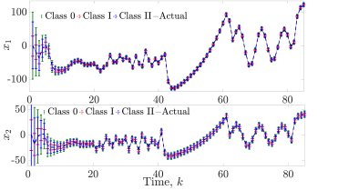
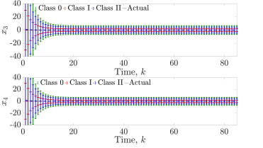
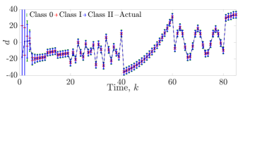
Figure 2: Actual states $x_{1}$,$x_{2}$,$x_{3}$,$x_{4}$ and input $d$, as well as their Class $0$, Class I and Class II estimates (i.e., the obtained estimates by applying the corresponding gains for Classes 0–II in Theorem 30).

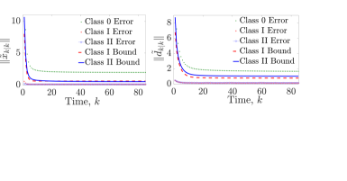
Figure 3: Estimation errors and their upper bounds for Class $0$ (${(\mathcal{M},\gamma)}$-QC), Class I (Lipschitz) and Class II (${(\mathcal{A},\gamma)}$-QC*) functions.

6.2 Comparison with Benchmark Observers

In this section, we illustrate the effectiveness of our Simultaneous Input and State Set-Valued Observer (SISO), by comparing its performance with two benchmark observers in [8] and [10]. The designed estimator in [8] calculates both (point) state and unknown input estimates, while the observer in [10], only obtains (point) state estimates. For comparison, we apply all the three observers on a benchmark dynamical system in [8], which is in the form of (8) with $n=2$, $m=l=p=1$, $f(x)=\begin{bmatrix}-0.42x_{1}+x_{2}&\ &-0.6x_{1}-1.25\tanh(x_{1})\end{bmatrix}^{\top}$, $G=\begin{bmatrix}1&-0.65\end{bmatrix}^{\top}$,$B=D=H=0_{1\times 1}$, $C=\begin{bmatrix}0&1\end{bmatrix}$, $W=I$, $\eta_{w}=0.2$ and $\eta_{v}=0.1$. The vector field $f(\cdot)$ is Lipschitz continuous (i.e., Class I) with $L_{f}=1.1171$. We consider two scenarios for the unknown input. In the first, we consider a random signal with bounded norm, i.e., $\|d_{k}\|\leq 0.2$ for the unknown input $d_{k}$, while $d_{k}$ in the second scenario is a time-varying signal that becomes unbounded as time increases. As is demonstrated in Figures 4 and 5, in the first scenario, i.e., with bounded unknown inputs, the set estimates of our approach (i.e., SISO estimates) converge to steady-state values and the point estimates of the two benchmark approaches [8, 10] are within the predicted upper bounds and exhibit a convergent behavior for all 50 randomly chosen initial values (cf. Figure 5). In this scenario, the two benchmark approaches result in slightly better performance than SISO, since they benefit from the additional assumption of bounded input.

More interestingly, considering the second scenario, i.e., with unbounded unknown inputs, Figures 6 and 7 demonstrate that our set-valued estimates still converge, i.e., our observer remains stable for all 50 randomly chosen initial values, with $P^{\star}=\begin{bmatrix}1.8086&1.4022\\ 1.4022&5.2068\end{bmatrix}$, $Y^{\star}=\begin{bmatrix}-0.2282&0.6664\end{bmatrix}^{\top}$, $\tilde{L}^{\star}=\begin{bmatrix}-0.2604&0.2064\end{bmatrix}$, $\alpha^{\star}=0.8875$ and ${\rho^{\star}}={1.7336}$, while the estimates of the two benchmark approaches exceed the boundaries of the compatible sets of states and inputs after some time steps of our approach and display a divergent behavior for all the initial values (cf. Figure 7).

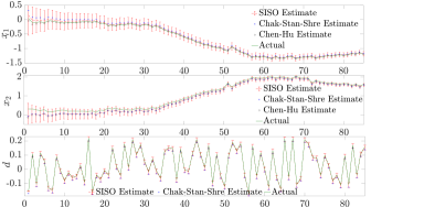
Figure 4: Actual states $x_{1}$, $x_{2}$, and their estimates, as well as unknown input $d$ and its estimates in the bounded unknown input scenario, obtained by applying the observer in [10] (Chen-Hu Estimate), the observer in [8] (Chak-Stan-Shre Estimate) and our proposed observer (SISO Estimate).

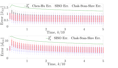
Figure 5: Estimation errors in the bounded unknown input scenario for 50 different initial values (using box plots), obtained by applying the observer in [10] (Chen-Hu Err.), the observer in [8] (Chak-Stan-Shre Err.) and our proposed observer (SISO Err.), as well as the computed upper bounds for the state and input errors ($\overline{\delta}^{x}_{k}$ and $\overline{\delta}^{d}_{k}$).

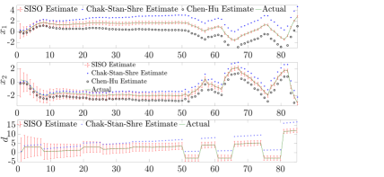
Figure 6: Actual states $x_{1}$, $x_{2}$, and their estimates, as well as unknown input $d$ and its estimates in the unbounded unknown input scenario, obtained by applying the observer in [10] (Chen-Hu Estimate), the observer in [8] (Chak-Stan-Shre Estimate) and our proposed observer (SISO Estimate).

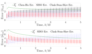
Figure 7: Estimation errors in the unbounded unknown input scenario for 50 different initial values (using box plots), obtained by applying the observer in [10] (Chen-Hu Err.), the observer in [8] (Chak-Stan-Shre Err.) and our proposed observer (SISO Err.), as well as the computed upper bounds for the state and input errors ( $\overline{\delta}^{x}_{k}$ and $\overline{\delta}^{d}_{k}$).

7 Conclusion and Future Work

We presented fixed-order set-valued $\mathcal{H}_{\infty}$-observers for nonlinear bounded-error discrete-time dynamic systems with unknown inputs. Necessary and sufficient Linear Matrix Inequalities for quadratic stability of the designed observer were derived for different classes of nonlinear systems, including ${(\mathcal{M},\gamma)}$-QC systems, Lipschitz continuous systems, ${(\mathcal{A},\gamma)}$-QC* systems and Linear Parameter-Varying systems. Moreover, we derived additional LMI conditions and corresponding tractable semi-definite programs for obtaining the minimum $\mathcal{H}_{\infty}$-norm for the transfer function that maps the noise signal to the state error of the stable observers.

In addition, we showed that the sequences of estimate radii of our $\mathcal{H}_{\infty}$-observer are uniformly bounded and derived closed- form expressions for their upper bound sequences. Further, we obtained sufficient conditions for the convergence of the radii upper bound sequences and derived their steady-state values. Finally, using two illustrative examples, we demonstrated the effectiveness of our proposed design, as well as its advantages over two existing benchmark observers. For future work, we plan to generalize this framework to hybrid and switched nonlinear systems and consider other forms of CPS attacks.

Appendix A Appendix

A.1 System Transformation

Let $p_{H}\triangleq{\rm rk}(H)$. Using singular value decomposition, we rewrite the direct feedthrough matrix $H$ as $H=\begin{bmatrix}U_{1}&U_{2}\end{bmatrix}\begin{bmatrix}\Sigma&0\\ 0&0\end{bmatrix}\begin{bmatrix}V_{1}^{\,\top}\\ V_{2}^{\,\top}\end{bmatrix}$, where $\Sigma\in\mathbb{R}^{p_{H}\times p_{H}}$ is a diagonal matrix of full rank, $U_{1}\in\mathbb{R}^{l\times p_{H}}$, $U_{2}\in\mathbb{R}^{l\times(l-p_{H})}$, $V_{1}\in\mathbb{R}^{p\times p_{H}}$ and $V_{2}\in\mathbb{R}^{p\times(p-p_{H})}$, while $U\triangleq\begin{bmatrix}U_{1}&U_{2}\end{bmatrix}$ and $V\triangleq\begin{bmatrix}V_{1}&V_{2}\end{bmatrix}$ are unitary matrices. When there is no direct feedthrough, $\Sigma$, $U_{1}$ and $V_{1}$ are empty matrices, and $U_{2}$ and $V_{2}$ are arbitrary unitary matrices, while when $p_{H}=p=l$, $U_{2}$ and $V_{2}$ are empty matrices, and $U_{1}$ and $\Sigma$ are identity matrices.

Then, we decouple the unknown input into two orthogonal components:

$$d_{1,k}=V_{1}^{\top}d_{k},\quad d_{2,k}=V_{2}^{\top}d_{k}.$$ (62)

Considering that $V$ is unitary,

$$d_{k}=V_{1}d_{1,k}+V_{2}d_{2,k},$$ (63)

and we can represent the system (16) as:

$$\begin{array}[]{rl}x_{k+1}&=f_{k}(x_{k})+B_{k}u_{k}+G_{1}d_{1,k}+G_{2}d_{2,k}+Ww_{k},\\ y_{k}&={C}x_{k}+D_{k}u_{k}+H_{1}d_{1,k}+v_{k},\end{array}$$ (66)

where $G_{1}\triangleq GV_{1}$, $G_{2}\triangleq GV_{2}$ and $H_{1}\triangleq HV_{1}=U_{1}\Sigma$. Next, the output $y_{k}$ is decoupled using a nonsingular transformation $T=\begin{bmatrix}T_{1}^{\top}&T_{2}^{\top}\end{bmatrix}^{\top}\triangleq U^{\top}=\begin{bmatrix}U_{1}&U_{2}\end{bmatrix}^{\top}$ to obtain $z_{1,k}\in\mathbb{R}^{p_{H}}$ and $z_{2,k}\in\mathbb{R}^{l-p_{H}}$ given by

$$\begin{array}[]{lll}z_{1,k}&\triangleq T_{1}y_{k}=U_{1}^{\top}y_{k}\\ &={C}_{1}x_{k}+\Sigma d_{1,k}+{D}_{k,1}u_{k}+{v}_{1,k},\\ z_{2,k}&\triangleq T_{2}y_{k}=U_{2}^{\top}y_{k}\\ &={C}_{2}x_{k}+{D}_{k,2}u_{k}+{v}_{2,k},\end{array}$$ (71)

where ${C}_{1}\triangleq U_{1}^{\top}{C}$, ${C}_{2}\triangleq U_{2}^{\top}{C}$, ${D}_{k,1}\triangleq U_{1}^{\top}{D}_{k}$, ${D}_{k,2}\triangleq U_{2}^{\top}{D}_{k}$, ${v}_{1,k}\triangleq U_{1}^{\top}{v}_{k}$ and ${v}_{2,k}\triangleq U_{2}^{\top}{v}_{k}$. This transformation is also chosen such that $\|\begin{bmatrix}{{v}_{1,k}}^{\top}&{{v}_{2,k}}^{\top}\end{bmatrix}^{\top}\|=\|U^{\top}{v}_{k}\|=\|{v}_{k}\|$. As a result, we obtain the transformed system (20).

A.2 Proofs

Next, we provide proofs for our propositions, lemmas and theorems. First, for the sake of reader’s convenience, we restate a lemma from [46] that we will frequently use in deriving some of our results.

Lemma 37.

[46, Lemma 2.2] Let $D$, $S$ and $F$ be real matrices of appropriate dimensions and $F^{\top}F\preceq I$. Then, for any scalar $\varepsilon>0$ and $x,y\in\mathbb{R}^{n}$,

$$2x^{\top}DFSy\leq\varepsilon^{-1}x^{\top}DD^{\top}x+\varepsilon y^{\top}S^{\top}Sy.$$

A.3 Proof of Proposition 7

The results follow from the facts that an inequality in $\mathbb{R}$ is preserved by multiplying the both sides by a non-negative number, or by multiplying the left hand side by a non-negative number that is not greater than 1, or by increasing the right hand side, as well as $A\preceq B\implies x^{\top}(A-B)x\preceq 0$. $\square$

A.4 Proof of Proposition 8

Considering $M=\begin{bmatrix}-I&0\\ 0&L^{2}_{f}\end{bmatrix}$, we have $\begin{bmatrix}\Delta f_{k}^{\top}&\Delta q^{\top}\end{bmatrix}{M}$ $\begin{bmatrix}\Delta f_{k}^{\top}&\Delta q^{\top}\end{bmatrix}^{\top}=-\Delta f_{k}^{\top}\Delta f_{k}+L^{2}_{f}\Delta q^{\top}\Delta q\geq 0$, where the inequality is implied by the Lipschitz continuity of $f_{k}(\cdot)$. $\square$

A.5 Proof of Proposition 9

By definition, $f_{k}(\cdot)$ is $\delta$-QC with multiplier matrix $M$ means that $\begin{bmatrix}\Delta f_{k}^{\top}&\Delta q^{\top}\end{bmatrix}$ ${M}\begin{bmatrix}\Delta f_{k}^{\top}&\Delta q^{\top}\end{bmatrix}^{\top}\geq 0$. Then, it follows in a straightforward manner that $\begin{bmatrix}\Delta f_{k}^{\top}&\Delta q^{\top}\end{bmatrix}({-M})\begin{bmatrix}\Delta f_{k}^{\top}&\Delta q^{\top}\end{bmatrix}^{\top}\leq\gamma$ for every $\gamma\geq 0$. $\square$

A.6 Proof of Proposition 12

We observe that $\begin{bmatrix}\Delta f_{k}^{\top}&\Delta x^{\top}\end{bmatrix}\mathcal{M}\begin{bmatrix}\Delta f_{k}^{\top}&\Delta x^{\top}\end{bmatrix}^{\top}$ $=-\Delta f_{k}^{\top}\Delta f_{k}$$\geq$ $-L^{2}_{f}\|\Delta x\|^{2}$$\geq-L^{2}_{f}(2r)^{2}=-4r^{2}L^{2}_{f}$, where the second and third inequalities hold by Lipschitz continuity of $f(\cdot)$ and boundedness of the state space, respectively. $\square$

A.7 Proof of Proposition 13

It follows from Definitions 6 and 11 and $\gamma\geq 0$ that

$$-\Delta f_{k}^{\top}\Delta f_{k}+2\Delta f_{k}^{\top}\mathcal{A}\Delta x-\Delta x^{\top}\mathcal{A}^{\top}\mathcal{A}\Delta x\geq\gamma\geq 0.$$

This, along with Lemma 37, imply that

$$(1-\epsilon) \|\Delta f_{k}\|^{2}\leq(\epsilon^{-1}-1)\Delta x^{\top}\mathcal{A}^{\top}\mathcal{A}\Delta x,\quad\forall\epsilon>0$$

$$\Rightarrow \|\Delta f_{k}\|^{2}\leq\frac{1}{\epsilon}\Delta x^{\top}\mathcal{A}^{\top}\mathcal{A}\Delta x,\quad\forall 0<\epsilon<1.$$

By taking the limit of the both sides when $\epsilon\to 1$ and by the continuity of the ”$\leq$” operator, we obtain

$$\|\Delta f_{k}\|^{2}\leq\Delta x^{\top}\mathcal{A}^{\top}\mathcal{A}\Delta x\leq\lambda_{\max}(\mathcal{A}^{\top}\mathcal{A})\|\Delta x\|^{2}.$$

Finally, the result is obtained by taking the square root of both sides of the above inequality. $\square$

A.8 Proof of Lemma 14

First, notice that $\Delta f_{k}=A\Delta x+\Delta g$. Given this and $\|g(x)\|\leq r$, we can conclude that

$$\begin{bmatrix}\Delta f_{k}^{\top}&\Delta x^{\top}\end{bmatrix}\mathcal{M}\begin{bmatrix}\Delta f_{k}^{\top}&\Delta x^{\top}\end{bmatrix}^{\top}$$

$$=-\Delta f_{k}^{\top}\Delta f_{k}+2\Delta x^{\top}A^{\top}\Delta f_{k}-\Delta x^{\top}A^{\top}A\Delta x$$

$$=-(\Delta f_{k}-A\Delta x)^{\top}(\Delta f_{k}-A\Delta x)=-\Delta g^{\top}\Delta g\geq-(2r)^{2}.\ \hfill\square$$

A.9 Proof of Proposition 15

By construction, we have the following condition: $\mathcal{M}-\begin{bmatrix}-I_{n\times n}&\mathcal{A}\\ \mathcal{A}^{\top}&-\mathcal{A}^{\top}\mathcal{A}\end{bmatrix}=\begin{bmatrix}\mathcal{M}_{11}+I&0\\ 0&\mathcal{M}_{22}+\mathcal{M}^{\top}_{12}\mathcal{M}_{12}\end{bmatrix}\preceq 0$, since both submatrices on the diagonal are negaitive semi-definite by assumption. $\square$

A.10 Proof of Proposition 16

The global Lipschitz continuity of LPV systems can be shown as follows:

$$\Delta f_{k} \triangleq\|f_{k}(x_{1})-f_{k}(x_{2})\|=\|\textstyle{\sum}_{i=1}^{N}\lambda_{i,k}A^{i}\Delta x_{k}\|$$

$$\leq\textstyle{\sum}_{i=1}^{N}\lambda_{i,k}\|A^{i}\Delta x_{k}\|\leq\textstyle{\sum}_{i=1}^{N}\lambda_{i,k}\|A^{i}\|\|\Delta x_{k}\|$$

$$\leq\|A^{m}\|\|\Delta x_{k}\|,$$

with $\|A^{m}\|=\max_{i\in{1\dots N}}\|A^{i}\|$, where the first and second inequalities hold by sub-multiplicative inequality for norms and positivity of $\lambda_{i,k}$, the third inequality holds by the facts that $0\leq\lambda_{i,k}\leq 1$ and $\textstyle{\sum}_{i=1}^{N}\lambda_{i,k}=1$. $\square$

A.11 Proof of Lemma 21

Aiming to derive the governing equation for the evolution of the state errors, from (71) and (21), we obtain

$$\hat{d}_{1,k}=M_{1}({C}_{1}\tilde{x}_{k|k}+\Sigma d_{1,k}+{v}_{1,k}).$$ (72)

Moreover, from (8), (71) and (22)–(25), we have

$$\hat{d}_{2,k-1} =M_{2}[C_{2}(\Delta f_{k-1}+G_{1}\tilde{d}_{1,k-1}+G_{2}d_{2,k-1}$$

$$\quad\quad\quad+Ww_{k-1})+v_{2,k}],$$ (73)

and by plugging $M_{1}=\Sigma^{-1}$ into (72), we obtain

$$\tilde{d}_{1,k}=d_{1,k}-\hat{d}_{1,k}=-M_{1}({C}_{1}\tilde{x}_{k|k}+{v}_{1,k}),$$ (74)

where $\Delta f_{k}\triangleq f_{k}(x_{k})-f_{k}(\hat{x}_{k})$. Then, by setting $M_{2}=(C_{2}G_{2})^{\dagger}$ in (A.11) and using (74), we have

$$\tilde{d}_{2,k-1}= -M_{2}[C_{2}(\Delta f_{k-1}-G_{1}M_{1}$$ (75)

$$(C_{1}\tilde{x}_{k-1|k-1}+v_{1,k-1})+Ww_{k-1})+{v}_{2,k}].$$

Furthermore, it follows from (8),(24) and (25) that

$$\textstyle\tilde{x}^{\star}_{k|k}=\Delta f_{k-1}+G_{1}\tilde{d}_{1,k-1}+\textstyle G_{2}\tilde{d}_{2,k-1}+W{w}_{k-1}.$$ (76)

In addition, by plugging $\tilde{d}_{k-1}$ and $\tilde{d}_{k-2}$ from (74) and (75) into (76), by (71) and (28), we obtain

$$\tilde{x}_{k|k} =(I-\tilde{L}C_{2})\tilde{x}^{\star}_{k|k}-\tilde{L}\tilde{v}_{k}.$$ (77)

$$\textstyle\tilde{x}^{\star}_{k|k} =\Phi[\Delta f_{k-1}-G_{1}M_{1}C_{1}\tilde{x}_{k-1|k-1}]+\textstyle\tilde{w}_{k},$$ (78)

where $\tilde{v}_{k}\triangleq v_{2,k}$, $\tilde{w}_{k}\triangleq-\Phi(G_{1}M_{1}v_{1,k-1}-Ww_{k-1})-G_{2}M_{2}v_{2,k}$ and $\Phi\triangleq I-G_{2}M_{2}C_{2}$. Finally, combining (77) and (78) returns the results. $\square$

A.12 Proof of Theorem 24

First, note that the state error dynamics (29) without bounded noise signals $w_{k}$ and $v_{k}$ can be rewritten as

$$\tilde{x}_{k+1|k+1}=\breve{A}\tilde{x}_{k|k}+\breve{B}\Delta f_{k},$$ (79)

with $\breve{A}\triangleq-(I-\tilde{L}C_{2})\Phi\Psi$ and $\breve{B}\triangleq(I-\tilde{L}C_{2})\Phi$. Moreover, considering a quadratic positive definite candidate Lyapunov function

$$V^{wn}_{k}=\tilde{x}_{k|k}^{\top}P\tilde{x}_{k|k},$$ (80)

with $P\succ 0$, (30) is equivalent to:

$$(\breve{A}\tilde{x}_{k|k}+\breve{B}\Delta f_{k})^{\top}P(\breve{A}\tilde{x}_{k|k}+\breve{B}\Delta f_{k})\leq(1-\alpha)\tilde{x}_{k|k}^{\top}P\tilde{x}_{k|k},$$

which can be reorganized as:

$$\begin{bmatrix}\Delta f_{k}\\ \tilde{x}_{k|k}\end{bmatrix}^{\top}\begin{bmatrix}\breve{B}^{\top}P\breve{B}&\breve{B}^{\top}P\breve{A}\\ \breve{A}^{\top}P\breve{B}&\breve{A}^{\top}P\breve{A}+(\alpha-1)P\end{bmatrix}\begin{bmatrix}\Delta f_{k}\\ \tilde{x}_{k|k}\end{bmatrix}\leq 0.$$ (81)

Then, for Class 0 functions (i.e., $(\mathcal{M},\gamma)$-QC functions), by Definition 6, we have

$$\begin{bmatrix}\Delta f_{k}\\ \tilde{x}_{k|k}\end{bmatrix}^{\top}\begin{bmatrix}-M_{11}&-M_{12}\\ -M^{\top}_{12}&-M_{22}\end{bmatrix}\begin{bmatrix}\Delta f_{k}\\ \tilde{x}_{k|k}\end{bmatrix}\leq-\gamma.$$ (82)

In other words, we want (81) to hold for any pair of $(\tilde{x}_{k|k},\Delta f_{k})$ that satisfy (82). By applying $\mathcal{S}$-procedure [48], this is equivalent to the existence of $\kappa\geq 0$, such that:

$$\kappa\begin{bmatrix}-M_{11}&-M_{12}&0\\ -M^{\top}_{12}&-M_{22}&0\\ 0&0&\gamma\end{bmatrix}-\begin{bmatrix}\breve{B}^{\top}P\breve{B}&\breve{B}^{\top}P\breve{A}&0\\ \breve{A}^{\top}P\breve{B}&\breve{A}^{\top}P\breve{A}+(\alpha-1)P&0\\ 0&0&0\end{bmatrix}\succeq 0.$$ (83)

Since $\gamma\geq 0$ by assumption, the above is equivalent to:

$$\exists\kappa\geq 0:\kappa\begin{bmatrix}-M_{11}&-M_{12}\\ -M^{\top}_{12}&-M_{22}\end{bmatrix}-\begin{bmatrix}\breve{B}^{\top}P\breve{B}&\breve{B}^{\top}P\breve{A}\\ \breve{A}^{\top}P\breve{B}&\breve{A}^{\top}P\breve{A}+(\alpha-1)P\end{bmatrix}\succeq 0.$$

Now, note that $\kappa=0$ is not a valid choice, since if $\kappa=0$, it can be shown that there is no $P\succ 0$ that satisfies the above inequality. Hence, $\kappa>0$, and we equivalently obtain $\exists P\succ 0,\kappa>0$, such that

$$\begin{bmatrix}\breve{B}^{\top}P\breve{B}&\breve{B}^{\top}P\breve{A}\\ \breve{A}^{\top}P\breve{B}&\breve{A}^{\top}P\breve{A}+(\alpha-1)P\end{bmatrix}\preceq{\color[rgb]{0,0,0}\kappa}\begin{bmatrix}-M_{11}&-M_{12}\\ -M^{\top}_{12}&-M_{22}\end{bmatrix}$$

$$\Leftrightarrow\begin{bmatrix}-{\color[rgb]{0,0,0}\kappa}M_{11}-\breve{B}^{\top}P\breve{B}&-{\color[rgb]{0,0,0}\kappa}M_{12}-\breve{B}^{\top}P\breve{A}\\ -{\color[rgb]{0,0,0}\kappa}M^{\top}_{12}-\breve{A}^{\top}P\breve{B}&-{\color[rgb]{0,0,0}\kappa}M_{22}-\breve{A}^{\top}P\breve{A}+(1-\alpha)P\end{bmatrix}\succeq 0,$$

which is, in turn, equivalent to:

$$\forall\epsilon>0{\color[rgb]{0,0,0},\exists P\succ 0,\kappa>0}:$$

$$\begin{bmatrix}-{\color[rgb]{0,0,0}\kappa}M_{11}-\breve{B}^{\top}P\breve{B}+\epsilon I&-{\color[rgb]{0,0,0}\kappa}M_{12}-\breve{B}^{\top}P\breve{A}\\ -{\color[rgb]{0,0,0}\kappa}M^{\top}_{12}-\breve{A}^{\top}P\breve{B}&-{\color[rgb]{0,0,0}\kappa}M_{22}-\breve{A}^{\top}P\breve{A}+(1-\alpha)P+\epsilon I\end{bmatrix}\succ 0.$$

Then, by applying Schur complement, we obtain

$$\forall\epsilon>0:\begin{cases}\tilde{M}_{22}\succ\tilde{M}_{12},\\ -{\color[rgb]{0,0,0}\kappa}M_{11}-\breve{B}^{\top}P\breve{B}+\epsilon I\succ 0,\end{cases}$$ (84)

with $\tilde{M}_{22}\triangleq-{\color[rgb]{0,0,0}\kappa}M_{22}-\breve{A}^{\top}P\breve{A}+(1-\alpha)P+\epsilon I$ and $\tilde{M}_{12}\triangleq({\color[rgb]{0,0,0}\kappa}M_{12}^{\top}+\breve{A}^{\top}P\breve{B})(-{\color[rgb]{0,0,0}\kappa}M_{11}-\breve{B}^{\top}P\breve{B}+\epsilon I)^{-1}({\color[rgb]{0,0,0}\kappa}M_{12}+\breve{B}^{\top}P\breve{A})$, where the second inequality is equivalent to:

$$-{\color[rgb]{0,0,0}\kappa}M_{11}-\breve{B}^{\top}PP^{-1}P\breve{B}\succeq 0\Leftrightarrow\begin{bmatrix}P&P\breve{B}\\ \breve{B}^{\top}P&-{\color[rgb]{0,0,0}\kappa}M_{11}\end{bmatrix}\succeq 0.$$

On the other hand, $\forall\epsilon>0:\tilde{M}_{22}\succ\tilde{M}_{12}$ is equivalent to:

$$\forall\epsilon>0,\exists\tilde{\Gamma}\succeq 0:$$

$$\begin{cases}\tilde{\Gamma}\succeq\tilde{M}_{12}\succeq 0,\\ -{\color[rgb]{0,0,0}\kappa}M_{22}-\breve{A}^{\top}PP^{-1}P\breve{A}+(1-\alpha)P+\epsilon I\succ\tilde{\Gamma}.\end{cases}$$ (85)

Since the second inequality holds for all $\epsilon$, it is equivalent to $-{\color[rgb]{0,0,0}\kappa}M_{22}-\breve{A}^{\top}PP^{-1}P\breve{A}+(1-\alpha)P\succeq\tilde{\Gamma}$, which, by applying Schur complement, is equivalent to:

$$\begin{bmatrix}P&P\breve{A}\\ \breve{A}^{\top}P&-{\color[rgb]{0,0,0}\kappa}M_{22}+(1-\alpha)P-\tilde{\Gamma}\end{bmatrix}\succeq 0.$$ (86)

By also applying Schur complement to (A.12), we obtain

$$\forall\epsilon{\color[rgb]{0,0,0}>0}:\tilde{\Gamma}\succeq\tilde{M}_{12}$$

$$\Leftrightarrow\forall\epsilon>0:\begin{bmatrix}-{\color[rgb]{0,0,0}\kappa}M_{11}-\breve{B}^{\top}P\breve{B}+\epsilon I&{\color[rgb]{0,0,0}\kappa}M_{12}+\breve{B}^{\top}P\breve{A}\\ {\color[rgb]{0,0,0}\kappa}M_{12}^{\top}+\breve{A}^{\top}P\breve{B}&\tilde{\Gamma}\end{bmatrix}\succeq 0$$

$$\Leftrightarrow\forall\epsilon>0:\begin{bmatrix}\tilde{\Gamma}&{\color[rgb]{0,0,0}\kappa}M_{12}^{\top}+\breve{A}^{\top}P\breve{B}\\ {\color[rgb]{0,0,0}\kappa}M_{12}+\breve{B}^{\top}P\breve{A}&-{\color[rgb]{0,0,0}\kappa}M_{11}-\breve{B}^{\top}P\breve{B}+\epsilon I\end{bmatrix}\succeq 0$$

$$\Leftrightarrow\forall\epsilon,\delta>0:$$

$$\quad\ \ \begin{bmatrix}\tilde{\Gamma}+\delta I&{\color[rgb]{0,0,0}\kappa}M_{12}^{\top}+\breve{A}^{\top}P\breve{B}\\ {\color[rgb]{0,0,0}\kappa}M_{12}+\breve{B}^{\top}P\breve{A}&\ -{\color[rgb]{0,0,0}\kappa}M_{11}-\breve{B}^{\top}P\breve{B}+(\epsilon+\delta)I\end{bmatrix}\succ 0.$$

Applying Schur complement to the above yields

$$\forall\epsilon,\delta>0:$$

$$\tilde{\Gamma}+\delta I\succ 0\Leftrightarrow\tilde{\Gamma}\succeq 0\ {\color[rgb]{0,0,0}\wedge-\kappa}M_{11}-\breve{B}^{\top}P\breve{B}+(\epsilon+\delta)I\succ\Xi,$$

where $\Xi\triangleq({\color[rgb]{0,0,0}\kappa}M_{12}+\breve{B}^{\top}P\breve{A})(\tilde{\Gamma}+\delta I)^{-1}({\color[rgb]{0,0,0}\kappa}M_{12}^{\top}+\breve{A}^{\top}P\breve{B})$. Then, from the last inequality, we equivalently obtain: $\forall\epsilon,\delta>0:\exists\breve{Q}$ such that:

$$-{\color[rgb]{0,0,0}\kappa}M_{11}-\breve{B}^{\top}P\breve{B}+(\epsilon+\delta)I\succ\breve{Q}$$

$$\Leftrightarrow-{\color[rgb]{0,0,0}\kappa}M_{11}-\breve{B}^{\top}P\breve{B}\succeq\breve{Q}\Leftrightarrow\begin{bmatrix}P&P\breve{B}\\ \breve{B}^{\top}P&-{\color[rgb]{0,0,0}\kappa}M_{11}-\breve{Q}\end{bmatrix}\succeq 0$$ (87)

and $\breve{Q}\succeq({\color[rgb]{0,0,0}\kappa}M_{12}+\breve{B}^{\top}P\breve{A})(\tilde{\Gamma}+\delta I)^{-1}({\color[rgb]{0,0,0}\kappa}M_{12}^{\top}+\breve{A}^{\top}P\breve{B})$, which is equivalent to

$$\forall\delta>0:\begin{bmatrix}\tilde{\Gamma}+\delta I&-{\color[rgb]{0,0,0}\kappa}M_{12}^{\top}-\breve{A}^{\top}P\breve{B}\\ -{\color[rgb]{0,0,0}\kappa}M_{12}-\breve{B}^{\top}P\breve{A}&\breve{Q}\end{bmatrix}\succeq 0.$$ (88)

Furthermore, pre - and post -multiplication of (88) by $\begin{bmatrix}I&0\\ 0&\Psi^{\top}\end{bmatrix}$ and $\begin{bmatrix}I&0\\ 0&\Psi\end{bmatrix}$, as well as the fact that $-\breve{B}\Psi=\breve{A}$ by definition and applying Schur complement, lead to

$$\forall\delta>0:\begin{bmatrix}\tilde{\Gamma}+\delta I&-{\color[rgb]{0,0,0}\kappa}M_{12}^{\top}\Psi+\breve{A}^{\top}P\breve{A}\\ -\Psi^{\top}{\color[rgb]{0,0,0}\kappa}M_{12}+\breve{A}^{\top}P\breve{A}&\Psi^{\top}\breve{Q}\Psi\end{bmatrix}\succeq 0$$

$$\Leftrightarrow\forall\delta>0:\Psi^{\top}\breve{Q}\Psi\succeq\tilde{Q},$$

where $\tilde{Q}\triangleq(-\Psi^{\top}{\color[rgb]{0,0,0}\kappa}M_{12}+\breve{A}^{\top}P\breve{A})(\tilde{\Gamma}+\delta I)^{-1}(-{\color[rgb]{0,0,0}\kappa}M_{12}^{\top}\Psi+\breve{A}^{\top}P\breve{A})$. Equivalently, we can represent this as:

$$\forall\delta>0,\exists\breve{Z}:$$

$$\breve{Z}\succeq-{\color[rgb]{0,0,0}\kappa}M_{12}^{\top}\Psi+\breve{A}^{\top}P\breve{A},\ \Psi^{\top}\breve{Q}\Psi\succeq\breve{Z}^{\top}(\tilde{\Gamma}+\delta I)^{-1}\breve{Z},$$

where the first inequality is equivalent to:

$$\begin{bmatrix}P&P\breve{A}\\ \breve{A}^{\top}P&\ \breve{Z}+{\color[rgb]{0,0,0}\kappa}M_{12}^{\top}\Psi\end{bmatrix}\succeq 0,$$

and the second inequality can be written as:

$$\forall\delta>0:\begin{bmatrix}\tilde{\Gamma}+\delta I&\breve{Z}\\ \breve{Z}^{\top}&\Psi^{\top}\breve{Q}\Psi\end{bmatrix}\succeq 0\Leftrightarrow\begin{bmatrix}\tilde{\Gamma}&\breve{Z}\\ \breve{Z}^{\top}&\Psi^{\top}\breve{Q}\Psi\end{bmatrix}\succeq 0,$$ (89)

where the forward direction (i.e., “$\Rightarrow$”) follows from the fact that the limit of a convergent sequence of positive semi-definite matrices is a positive semi-definite matrix, while the backward direction (i.e., “$\Leftarrow$”) holds since the summation of two positive semi-definite matrices is positive semi-definite. Finally, by defining $Y\triangleq P\tilde{L}$ with $\tilde{\Gamma}\succ 0$ and the LMIs in (84)–(A.12) and (A.12), we obtain the results for Class 0 functions.

Next, we consider system classes I–III by appealing to the fact that they are Class 0 systems with additional information about $M_{11},M_{12}$ and $M_{22}$:

• Case I: From Proposition 8, we can replace $M_{11},M_{12}$ and $M_{22}$ with $-I,0_{n\times n}$ and $L_{f}^{2}I$.

• Case II: By Definition 11, we can substitute $M_{11},M_{12}$ and $M_{22}$ with $-I,\mathcal{A}$ and $-\mathcal{A}^{\top}\mathcal{A}$.

• Case III: Note that by Proposition 16, an LPV function is Lipschitz continuous by Lipschitz constant $\tilde{\sigma}_{m}\triangleq\max_{i\in{1\dots N}}\|A^{i}\|$. Hence, we can apply Case I by replacing $L_{f}$ with $\tilde{\sigma}_{m}$.

Finally, suppose $\gamma<0$. Then, the fact that $\kappa=0$ is not a valid choice (as previously discussed) implies that $\kappa\gamma<0$ and hence, the matrix in the left hand side of (83) always contains a strictly negative diagonal element $\kappa\gamma<0$ and consequently, (83) can never hold, and thus, neither can (81). $\square$

A.13 Proof of Proposition 26

To prove the necessity of (45), we use contraposition. Suppose that the LMIs in (45) are feasible. Then, we will show that there exists a candidate Lyapunov function $\tilde{V}^{wn}_{k}=\tilde{x}^{\top}_{k|k}\tilde{P}\tilde{x}_{k|k}$, for some $\tilde{P}\succ 0$, such that $\Delta\tilde{V}^{wn}_{k}\triangleq\tilde{V}^{wn}_{k+1}-\tilde{V}^{wn}_{k}\succ 0$ and hence, by the Lyapunov instability theorem [26, Theorem 3.3], the error system is unstable. Therefore, the conditions in (45) are necessary for the stability of the observer. To do so, first note that

$$\Delta\tilde{V}^{wn}_{k} =\Delta f^{\top}_{k}\Phi^{\top}(I-\tilde{L}C_{2})^{\top}\tilde{P}(I-\tilde{L}C_{2})\Phi\Delta f_{k}$$ (90)

$$+\tilde{x}^{\top}_{k|k}(\Psi^{\top}\Phi^{\top}(I-\tilde{L}C_{2})^{\top}\tilde{P}(I-\tilde{L}C_{2})\Phi\Psi-\tilde{P})\tilde{x}_{k|k}$$

$$-2\Delta f^{\top}_{k}\Phi^{\top}(I-\tilde{L}C_{2})^{\top}\tilde{P}(I-\tilde{L}C_{2})\Phi\Psi\tilde{x}_{k|k}.$$

Then, (45), along with setting $\tilde{L}=\tilde{P}^{-1}\tilde{Y}\Rightarrow\tilde{Y}=\tilde{P}\tilde{L}$, defining $\tilde{S}\triangleq\tilde{P}-C^{\top}_{2}\tilde{Y}^{\top}-\tilde{Y}C_{2}$, $\hat{\Pi}\succeq 0$ and applying Schur complement, result in

$$0\prec\tilde{L}^{\top}\tilde{P}\tilde{L}\preceq\tilde{\Gamma}\preceq I,$$ (91)

as well as

$$\Delta\tilde{V}^{wn}_{k}=\Delta f^{\top}_{k}\Phi^{\top}(\tilde{S}+C^{\top}_{2}\tilde{L}^{\top}\tilde{P}\tilde{L}C_{2})\Phi\Delta f_{k}$$ (92)

$$\ \ +\tilde{x}^{\top}_{k|k}(\Psi^{\top}\Phi^{\top}(\tilde{S}+C^{\top}_{2}\tilde{L}^{\top}\tilde{P}\tilde{L}C_{2})\Phi\Psi-\tilde{P})\tilde{x}_{k|k}$$

$$\ \ -2\Delta f^{\top}_{k}\Phi^{\top}\tilde{S}\Phi\Psi\tilde{x}_{k|k}-2\Delta f^{\top}_{k}\Phi^{\top}C^{\top}_{2}\tilde{L}^{\top}\tilde{P}\tilde{L}C_{2}\Phi\Psi\tilde{x}_{k|k}.$$

Then, (91), (92) and Lemma 37 imply that there exists $\tilde{\eta}>0$ such that

$$\begin{array}[]{rl}&\Delta\tilde{V}^{wn}_{k}\geq\Delta f^{\top}_{k}\Phi^{\top}(\tilde{S}+\tilde{\eta}C^{\top}_{2}C_{2})\Phi\Delta f_{k}\\ &\ \ +\tilde{x}^{\top}_{k|k}(\Psi^{\top}\Phi^{\top}(\tilde{S}+\tilde{\eta}C^{\top}_{2}C_{2})\Phi\Psi-\tilde{P})\tilde{x}_{k|k}\\ &\ \ -2\Delta f^{\top}_{k}\Phi^{\top}\tilde{S}\Phi\Psi\tilde{x}_{k|k}-\Delta f^{\top}_{k}\Phi^{\top}C^{\top}_{2}C_{2}\Phi\Delta f_{k}\\ &\ \ -\tilde{x}^{\top}_{k|k}\Psi^{\top}\Phi^{\top}C^{\top}_{2}C_{2}\Phi\Psi\tilde{x}_{k|k}\triangleq\overline{\Delta}\tilde{V}^{wn}_{k}.\end{array}$$ (97)

As with the proof of Theorem 24, we first consider Class 0 systems, where by plugging $\tilde{\Pi}_{11}$, $\tilde{\Pi}_{12}$ and $\tilde{\Pi}_{22}$ given in (49) into $\tilde{\Pi}$, as defined in (45), we obtain:

$$0<[\Delta f^{\top}_{k}\ \tilde{x}^{\top}_{k|k}]\tilde{\Pi}[\Delta f^{\top}_{k}\ \tilde{x}^{\top}_{k|k}]^{\top}=\overline{\Delta}\tilde{V}^{wn}_{k}-\delta_{f}$$ (98)

where

$$\delta_{f} \triangleq\Delta f_{k}^{\top}M_{11}\Delta f_{k}+2\tilde{x}_{k|k}^{\top}M_{12}^{\top}\Delta f_{k}+\tilde{x}_{k|k}^{\top}M_{22}\tilde{x}_{k|k}$$

$$=\begin{bmatrix}\Delta f_{k}^{\top}&\tilde{x}^{\top}_{k|k}\end{bmatrix}\mathcal{M}\begin{bmatrix}\Delta f_{k}^{\top}&\tilde{x}^{\top}_{k|k}\end{bmatrix}^{\top}\geq\gamma\geq 0.$$ (99)

Finally, from (97), we have $\Delta\tilde{V}^{wn}_{k}\geq\overline{\Delta}\tilde{V}^{wn}_{k}>\delta_{f}\geq 0\Rightarrow\Delta\tilde{V}^{wn}_{k}>0$.

Furthermore, the proof for system classes I–III can be obtained from the above result for Class 0 with suitable values of $M_{11}$, $M_{12}$ and $M_{22}$ as discussed in the proof of Theorem 24. $\square$

A.14 Proof of Lemma 27

To show that uniform detectability is sufficient for existence of an observer, notice that for a Class III function $f_{k}(\cdot)$, (29) can be written as

$$\tilde{x}_{k|k} =(I-\tilde{L}C_{2})\overline{A}_{k-1}\tilde{x}_{k-1|k-1}$$

$$+(I-\tilde{L}C_{2})\tilde{w}_{k-1}-\tilde{L}\tilde{v}_{k-1},$$ (100)

where

$$\tilde{w}_{k-1} \triangleq-(I-G_{2}M_{2}C_{2})(G_{1}M_{1}v_{1,k-1}-{w}_{k-1})$$

$$\quad-G_{2}M_{2}{v}_{2,k},$$

$$\overline{A}_{k} \triangleq\Phi(\sum_{i=1}^{N}\lambda_{i,k}{A}^{i}-\Psi),\quad\tilde{v}_{k-1}\triangleq{v}_{2,k}.$$

Now, consider the following linear time-varying system without unknown inputs:

$$x_{k+1}=\overline{A}_{k}x_{k}+\tilde{w}_{k},y_{k}=C_{2}x_{k}+\tilde{v}_{k}.$$ (101)

Systems (100) and (101) are equivalent from the viewpoint of estimation, since the estimation error equations for both problems are the same, hence they both have the same objective. Therefore, the pair $(\overline{A}_{k},C_{2})$ needs to be uniformly detectable such that the observer is stable [4, Section 5].

Moreover, as for the necessity of the strong detectability of the constituent LTI systems, suppose for contradiction, that there exists a stable observer for system (8) with any sequence $\{\lambda_{i,k}\}_{k=0}^{\infty}$ for all $i\in\{1,2,\dots,N\}$ that satisfies $0\leq\lambda_{i,k}\leq 1,\sum_{i=1}^{N}\lambda_{i,k}=1,\forall k$, but one of the constituent linear time-invariant systems (e.g., $({A}^{j},G,{C},H)$) is not strongly detectable. Since the observer exists for any sequence of $\lambda_{i,k}$, that means that an observer also exists when $\lambda_{j,k}=1$ and $\lambda_{i,k}=0$, $\forall i\neq j$ for all $k$. However, we know from [49] that strong detectability is necessary for the stability of the linear time-invariant system $({A}^{j},G,{C},H)$, which is a contradiction. Hence, the proof is complete. $\square$

A.15 Proof of Theorem 30

We use a similar approach as in the proof of Theorem 24. First, consider the error dynamics with bounded noise signals (29) and the candidate Lyapunov function $V^{n}_{k}\triangleq\tilde{x}^{\top}_{k|k}P\tilde{x}_{k|k}$. Observe that

$$\Delta V^{n}_{k}\triangleq V^{n}_{k+1}-V^{n}_{k}=\Delta V^{wn}_{k}+\Delta r_{k},$$ (102)

where $V^{wn}_{k}$ is the Lyapunov function for the error dynamics without noise signals, defined in (80), and

$$\Delta r_{k} \triangleq 2(\Delta f^{\top}_{k}-\tilde{x}^{\top}_{k|k}\Psi^{\top})\Phi^{\top}(I-\tilde{L}C_{2})^{\top}P\mathcal{W}(\tilde{L})\overline{w}_{k}$$

$$+\overline{w}^{\top}_{k}\mathcal{W}(\tilde{L})^{\top}P\mathcal{W}(\tilde{L})\overline{w}_{k},$$ (103)

with $\Phi,\Psi,\overline{w}_{k}$ and $\mathcal{W}(\tilde{L})$ defined in Lemma 21. We will show for each system class we consider that

$$\overline{\Delta}r_{k}\triangleq\Delta r_{k}-\rho^{2}\overline{w}^{\top}_{k}\overline{w}_{k}+\tilde{x}^{\top}_{k}(I-\alpha P)\tilde{x}_{k}\leq 0.$$ (104)

Then, by (102) and (104) in addition to the fact that $\Delta V^{wn}_{k}\leq-\alpha\tilde{x}^{\top}_{k}P\tilde{x}_{k}$ (follows from Theorem 24), we have

$$\Delta V^{n}_{k}\leq\rho^{2}\overline{w}^{\top}_{k}\overline{w}_{k}-\tilde{x}^{\top}_{k|k}\tilde{x}_{k|k}.$$ (105)

Summing up both sides of (105) from zero to infinity, returns $V^{n}_{\infty}-V^{n}_{0}\leq\rho^{2}\textstyle{\sum}_{k=0}^{\infty}\overline{w}^{\top}_{k}\overline{w}_{k}-\textstyle{\sum}_{k=0}^{\infty}\tilde{x}^{\top}_{k|k}\tilde{x}_{k|k}=\rho^{2}\textstyle{\sum}_{k=0}^{\infty}\vec{w}_{i}^{\top}\vec{w}_{i}-\textstyle{\sum}_{k=0}^{\infty}\tilde{x}^{\top}_{k|k}\tilde{x}_{k|k}$, where at each time step $k$, $\vec{w}^{\top}_{k}=\begin{bmatrix}w^{\top}_{k}&v^{\top}_{k}\end{bmatrix}^{\top}$. Then, it follows from setting the initial conditions to zero that $\textstyle{\sum}_{k=0}^{\infty}\tilde{x}^{\top}_{k|k}\tilde{x}_{k|k}\leq\rho^{2}\textstyle{\sum}_{k=0}^{\infty}\vec{w}_{i}^{\top}\vec{w}_{i}$.

Thus, it remains to show that (104) holds for each system class 0–III. Plugging the expression for $\mathcal{W}(\tilde{L})$ from Lemma 21 into (A.15), we obtain

$$\overline{\Delta}r_{k} =\tilde{x}^{\top}_{k|k}(I-\alpha P)\tilde{x}_{k|k}+2(\Delta f_{k}-\Psi\tilde{x}_{k|k})^{\top}\Phi^{\top}(PR$$

$$\quad-Y\Omega-C^{\top}_{2}Y^{\top}R+C^{\top}_{2}\tilde{L}^{\top}P\tilde{L}\Omega)\overline{w}_{k}+\overline{w}^{\top}_{k}(R^{\top}PR$$

$$\quad-2\Omega^{\top}Y^{\top}R+\Omega^{\top}\tilde{L}^{\top}P\tilde{L}\Omega-\rho^{2}I)\overline{w}_{k},$$ (106)

On the other hand, note that $\Pi\succeq 0\Leftrightarrow I-\Gamma\succeq 0$ and $\begin{bmatrix}\Gamma&Y^{\top}\\ Y&P\end{bmatrix}\succeq 0$, which by pre- and post-multiplication by $\begin{bmatrix}I&0\\ 0&P^{-1}\end{bmatrix}$ and the fact that $Y=P\tilde{L}$, is equivalent to $I-\Gamma\succeq 0$ and $\begin{bmatrix}\Gamma&\tilde{L}^{\top}\\ \tilde{L}&P^{-1}\end{bmatrix}\succeq 0$. Applying Schur complement to the latter, $\Pi\succeq 0$ is equivalent to

$$0\preceq\tilde{L}^{\top}P\tilde{L}\preceq\Gamma\preceq I.$$ (107)

Now, (A.15), (107) and Lemma 37, imply that:

$$\overline{\Delta}r_{k} \leq\overline{w}^{\top}_{k}(R^{\top}PR-2R^{\top}Y\Omega+\Omega^{\top}\Gamma\Omega+(\varepsilon^{-1}_{1}+\varepsilon^{-1}_{2})\Omega^{\top}\Omega$$

$$-\rho^{2}I)\overline{w}_{k}+\tilde{x}^{\top}_{k|k}(I-\alpha P+\varepsilon_{1}\Psi^{\top}\Phi^{\top}C^{\top}_{2}C_{2}\Phi\Psi)\tilde{x}_{k|k}$$

$$+2\Delta f^{\top}_{k}\Phi^{\top}(PR-Y\Omega-C^{\top}_{2}Y^{\top}R)\overline{w}_{k}$$

$$-2\tilde{x}^{\top}_{k|k}\Psi^{\top}\Phi^{\top}(PR-Y\Omega-C^{\top}_{2}Y^{\top}R)\overline{w}_{k}$$ (108)

$$+\varepsilon_{2}\Delta f^{\top}_{k}(\Phi^{\top}C^{\top}_{2}C_{2}\Phi)\Delta f_{k}\triangleq\tilde{\Delta}r_{k}.$$

We first consider Class 0 systems, where the fact that $f_{k}(\cdot)$ is ($\mathcal{M},\gamma$)-QC with $\gamma\geq 0$ implies that

$$-\Delta f^{\top}_{k}M_{11}\Delta f_{k}-\tilde{x}^{\top}_{k|k}M_{22}\tilde{x}_{k|k}-2\Delta f_{k}^{\top}M_{12}^{\top}\tilde{x}_{k|k}$$

$$\triangleq\tilde{S}\leq-\gamma\leq 0,$$

which, in addition to (108), return $\overline{\Delta}r_{k}\leq\tilde{\Delta}r_{k}-\tilde{S}+\tilde{S}=-\zeta^{\top}\mathcal{N}\zeta+\tilde{S}\leq 0$, where $\zeta\triangleq\begin{bmatrix}\overline{w}^{\top}_{k}&\tilde{x}^{\top}_{k}&\Delta f^{\top}_{k}\end{bmatrix}^{\top}$ and $\mathcal{N}$ is the matrix in (51) with its elements defined in (30) and ( ‣ 30). Finally, we can obtain the results for system classes I–III with suitable values of $M_{11}$, $M_{12}$ and $M_{22}$ as described in the proof of Theorem 24. $\square$

A.16 Proof of Theorem 32

Consider the noisy state error dynamics system in (29), where we treat the augmented noise signal $\overline{w}_{k}$ as an external input to the system. Recall from the proof of Theorem 30 that as a result of $\mathcal{H}_{\infty}$ observer design, the Lyapunov function $V^{n}_{k}\triangleq\tilde{x}^{\top}_{k|k}P\tilde{x}_{k|k}$ satisfies (105), which is equivalent to $\Delta V^{n}_{k}\leq-\alpha_{3}(\|\tilde{x}_{k|k}\|)+\sigma(\|\overline{w}_{k}\|)$, with the $\mathcal{K}_{\infty}$-function $\alpha_{3}(r)\triangleq r^{2}$ and the $\mathcal{K}$-function $\sigma(s)\triangleq\eta^{2}s^{2}$. This implies that $V^{n}_{k}$ is an ISS-Lyapunov function for system (29) (cf. [21, Definition 3.2]), i.e., (29) admits an Input-to-State Stable (ISS)-Lyapunov function. Equivalently, (29) is ISS and UBIBS, and admits a $\mathcal{K}$-asymptotic gain by [21, Theorem 1]. $\square$

A.17 Proof of Theorem 33

In this theorem, we aim to find two upper bounds of $\|\tilde{x}_{k|k}\|$ such that that $\|\tilde{x}_{k|k}\|\leq\overline{\delta}^{x}_{k,1}$ and $\|\tilde{x}_{k|k}\|\leq\overline{\delta}^{x}_{k,2}$. To derive the first upper bound, notice that it follows from (105) that

$$\tilde{x}^{\top}_{k|k}P\tilde{x}_{k|k}\leq\rho^{2}\overline{w}^{\top}_{k}\overline{w}_{k}+\tilde{x}^{\top}_{k-1|k-1}(P-I)\tilde{x}_{k-1|k-1},$$

and by applying Rayleigh’s inequality, we obtain

$$\lambda_{\min}(P)\|\tilde{x}_{k|k}\|^{2}\leq\rho^{2}\overline{w}^{\top}_{k}\overline{w}_{k}+\lambda_{\max}(P-I)\|\tilde{x}_{k-1|k-1}\|^{2}$$

$$\Rightarrow\|\tilde{x}_{k|k}\|\leq\sqrt{\frac{\rho^{2}\overline{w}^{\top}_{k}\overline{w}_{k}}{\lambda_{\min}(P)}+\frac{|\lambda_{\max}(P-I)|}{\lambda_{\min}(P)}\|\tilde{x}_{k-1|k-1}\|^{2}}.$$

Repeating this procedure $k$ times and considering the fact that $\lambda_{\max}(P-I)=\lambda_{\max}(P)-1$ as a consequence of Weyl’s Theorem [20, Theorem 4.3.1], we obtain $\tilde{x}_{k|k}\leq\overline{\delta}^{x}_{k,1}$ with $\overline{\delta}^{x}_{k,1}$ given in (56) and $\theta_{1}={\color[rgb]{0,0,0}\frac{|\lambda_{\max}(P)-1|}{\lambda_{\min}(P)}}$.

Next, we find the second upper bound for $\|\tilde{x}_{k|k}\|\leq\overline{\delta}^{x}_{k,2}\triangleq\delta^{x}_{0}\theta_{2}^{k}+\overline{\eta}\textstyle\sum_{i=1}^{k}\theta_{2}^{i-1}$ for system classes I–III.

1. If $f_{k}(\cdot)$ is a Class I function, then, the result in (58) with $\theta$ defined in (59), directly follows from Lipschitz continuity of $f_{k}(\cdot)$, as well as applying triangle and sub-multiplicative inequalities for norms on (29). Moreover, the result in (55) with $\beta$ defined in (59), is obtained by triangle and sub-multiplicative inequalities, (63), (74) and (75).
   

2. If $f_{k}(\cdot)$ is a Class II function, then by Proposition 13, it is a Class I function with $L_{f}=\sqrt{\lambda_{\max}(\mathcal{A}^{\top}\mathcal{A})}$. The rest of the proof is similar to the proof for Class I.

3. If $f_{k}(\cdot)$ is a Class III function, we first find closed-form expressions for the state and input estimation errors through the following lemma.
   

   Lemma 38.

   The state and input estimation errors are

   $$\tilde{x}_{k|k} =\sum_{i=1}^{k}\prod_{j=0}^{i-2}A_{e,k-j}(\Psi\tilde{w}_{k-i}-\tilde{L}\tilde{v}_{k-i})+\prod_{j=0}^{k-1}A_{e,k-j}\tilde{x}_{0|0},$$

   $$\tilde{d}_{k-1} =-\textstyle\sum_{i=1}^{N}\lambda_{i,k-1}(V_{1}M_{1}C_{1}+V_{2}M_{2}C_{2}A_{e,i})\tilde{x}_{k-1|k-1}$$

   $$\quad+(V_{2}M_{2}C_{2}G_{1}M_{1}-V_{1}M_{1})T_{1}v_{k-1}-V_{2}M_{2}C_{2}w_{k-1}$$

   $$\quad-V_{2}M_{2}T_{2}v_{k}.$$

   Proof A.1.

   Starting from (100) and applying simple induction return the results for the state errors. Then, the expression for the input errors follows from (74), (75) and (63).

   Now, we are ready to show that $\|\tilde{x}_{k|k}\|\leq\overline{\delta}^{x}_{k,2}\triangleq\delta^{x}_{0}\theta_{2}^{k}+\overline{\eta}\textstyle\sum_{i=1}^{k}\theta_{2}^{i-1}$ for LPV (Class III) functions. First, we define

   $$\begin{array}[]{c}B_{e,k}\triangleq\textstyle\prod_{j=0}^{k-1}A_{e,k-j},\\ C^{i}_{e,k}\triangleq\textstyle\prod_{j=0}^{i-2}A_{e,k-j},\ \tilde{t}_{k}\triangleq\Psi\tilde{w}_{k}-\tilde{L}\tilde{v}_{k},\end{array}$$ (111)

   for $1\leq i\leq k$. Then, from Lemma 38, we have

   $$\|\tilde{x}_{k|k}\|\leq\|B_{e,k}\|\|\tilde{x}_{0|0}\|+\|\textstyle\sum_{i=1}^{k}C^{i}_{e,k}\overline{t}_{k-i}\|,$$ (112)

   by triangle inequality and submultiplicativity of norms. Moreover, by a similar reasoning, we find

   $$\|B_{e,k}\|\leq\|\textstyle\prod_{j=0}^{k-1}\textstyle\sum_{i=1}^{N}\lambda^{i}_{k-j}\Psi\Phi(A^{i}-G_{1}M_{1}C_{1})\|\leq{\color[rgb]{0,0,0}\theta_{2}^{k}},$$

   $$\|\sum_{i=1}^{k}C^{i}_{e,k}\overline{t}_{k-i}\|\leq\sum_{i=1}^{k}\|C^{i}_{e,k}\|\|\overline{t}_{k-i}\|,$$ (113)

   $$\|C^{i}_{e,k}\|\leq\textstyle\prod_{j=0}^{i-2}\|\textstyle\sum_{s=1}^{N}\lambda_{s,k-j}A_{e,s}\|\leq\theta_{2}^{i-1}.$$

   Moreover, from (111), we have

   $$\|\tilde{t}_{k-i}\|=\|\Re v_{k-i}+\Psi\Phi w_{k-i}\|\leq\overline{\eta},$$ (114)

   with $\Re\triangleq-(\Psi\Phi G_{1}M_{1}T_{1}+\Psi G_{2}M_{2}T_{2}+\tilde{L}T_{2})$. Then, from (112)–(114), we obtain (58) with ${\color[rgb]{0,0,0}\theta_{2}}$ and $\overline{\eta}$ defined in (61). Furthermore, the result in (55) with $\beta$ and $\overline{\alpha}$ defined in (61), follows from applying Lemma 38, as well as triangle inequality, the facts that $0\leq\lambda_{i,k}\leq 1,\textstyle\sum_{i=1}^{N}\lambda_{i,k}=1$ and sub-multiplicativity of matrix norms.

Further, the steady state values are obtained by taking the limit from both sides of (56), (58) and (55), and assuming that $\theta\triangleq\min(\theta_{1},\theta_{2})<1$. $\square$

A.18 Proof of Corollary 34

Clearly $\|A_{e,i}\|<1$ implies that $\theta<1$, which is a sufficient condition for the convergence of errors by Theorem 33. $\square$

A.19 Proof of Proposition 36

The stability of the observer and the noise attenuation level follow directly from Theorems 27 and 30, respectively. Moreover, we will show that the additional LMIs

$$\kappa_{1}I\preceq P\preceq\kappa_{2}I,$$ (115)

$$(\kappa_{1}\geq 1,\kappa_{2}-\kappa_{1}<1)\ {\color[rgb]{0,0,0}\vee}\ (\kappa_{2}\leq 1,\kappa_{1}>0.5),$$ (116)

imply that $\theta_{1}\triangleq{\color[rgb]{0,0,0}{\frac{|\lambda_{\max}(P)-1|}{\lambda_{\min}(P)}}}<1$, which guarantees that $\theta=\min(\theta_{1},\theta_{2})<1$ and therefore, the radii upper sequences are convergent by Theorem 33. To do so, we consider two cases:

• Case A) $\kappa_{1}\geq 1,\kappa_{2}-\kappa_{1}<1$. This, along with (115) result in $\lambda_{\max}(P)\geq\kappa_{1}\geq 1$ and $|\lambda_{\max}(P)-1|=\lambda_{\max}(P)-1\leq\kappa_{2}-1<\kappa_{1}\leq\lambda_{\min}(P)$. Hence, $\theta_{1}\triangleq{\color[rgb]{0,0,0}{\frac{|\lambda_{\max}(P)-1|}{\lambda_{\min}(P)}}}<1$.

• Case B) $\kappa_{2}\leq 1,\kappa_{1}>0.5$. This, in addition to (115) return $\lambda_{\max}(P)\leq\kappa_{2}\leq 1$ and $|\lambda_{\max}(P)-1|=1-\lambda_{\max}(P)\leq 1-\kappa_{1}<\kappa_{1}\leq\lambda_{\min}(P)$. So, $\theta_{1}\triangleq{\color[rgb]{0,0,0}{\frac{|\lambda_{\max}(P)-1|}{\lambda_{\min}(P)}}}<1$. $\square$

References

- [1] M. Abolhasani and M. Rahmani. Robust deterministic least-squares filtering for uncertain time-varying nonlinear systems with unknown inputs. Systems & Control Letters, 122:1–11, 2018.
- [2] A. Acikmese and M. Corless. Stability analysis with quadratic lyapunov functions: A necessary and sufficient multiplier condition. In Proceedings of the Annual Allerton Conference on Communication, Control and Computing, volume 41, pages 1546–1555. Citeseer, 2003.
- [3] B. Açıkmeşe and M. Corless. Observers for systems with nonlinearities satisfying incremental quadratic constraints. Automatica, 47(7):1339–1348, 2011.
- [4] B.D.O. Anderson and J.B. Moore. Detectability and stabilizability of time-varying discrete-time linear systems. SIAM Journal on Control and Optimization, 19(1):20–32, 1981.
- [5] F. Blanchini and M. Sznaier. A convex optimization approach to synthesizing bounded complexity filters. IEEE Transactions on Automatic Control, 57(1):216–221, 2012.
- [6] A.A. Cárdenas, S. Amin, and S. Sastry. Research challenges for the security of control systems. In Conference on Hot Topics in Security, pages 6:1–6:6, 2008.
- [7] A. Chakrabarty and M. Corless. Estimating unbounded unknown inputs in nonlinear systems. Automatica, 104:57–66, 2019.
- [8] A. Chakrabarty, S.H. Żak, and S. Sundaram. State and unknown input observers for discrete-time nonlinear systems. In 2016 IEEE 55th Conference on Decision and Control (CDC), pages 7111–7116. IEEE, 2016.
- [9] K. Chandrasekar and M.S Hsiao. Implicit search-space aware cofactor expansion: A novel preimage computation technique. In 2006 International Conference on Computer Design, pages 280–285. IEEE, 2006.
- [10] B. Chen and G. Hu. Nonlinear state estimation under bounded noises. Automatica, 98:159–168, 2018.
- [11] J. Chen and C.M. Lagoa. Observer design for a class of switched systems. In IEEE Conference on Decision and Control European Control Conference, pages 2945–2950, 2005.
- [12] M.S. Chong, M. Wakaiki, and J.P. Hespanha. Observability of linear systems under adversarial attacks. In IEEE American Control Conference (ACC), pages 2439–2444, 2015.
- [13] G. De Nicolao, G. Sparacino, and C. Cobelli. Nonparametric input estimation in physiological systems: Problems, methods, and case studies. Automatica, 33(5):851–870, 1997.
- [14] J.P. Farwell and R. Rohozinski. Stuxnet and the future of cyber war. Survival, 53(1):23–40, 2011.
- [15] H. Fawzi, P. Tabuada, and S. Diggavi. Secure estimation and control for cyber-physical systems under adversarial attacks. IEEE Transactions on Automatic Control, 59(6):1454–1467, June 2014.
- [16] G. Garcia, J. Bernussou, and D. Arzelier. Robust stabilization of discrete-time linear systems with norm-bounded time-varying uncertainty. Systems & Control Letters, 22(5):327–339, 1994.
- [17] S. Gillijns and B. De Moor. Unbiased minimum-variance input and state estimation for linear discrete-time systems. Automatica, 43(1):111–116, January 2007.
- [18] S. Gillijns and B. De Moor. Unbiased minimum-variance input and state estimation for linear discrete-time systems with direct feedthrough. Automatica, 43(5):934–937, 2007.
- [19] Q.P. Ha and H. Trinh. State and input simultaneous estimation for a class of nonlinear systems. Automatica, 40(10):1779–1785, 2004.
- [20] R.A. Horn and C.R. Johnson. Matrix analysis. Cambridge University Press, 2012.
- [21] Z.P. Jiang and Y. Wang. Input-to-state stability for discrete-time nonlinear systems. Automatica, 37(6):857–869, 2001.
- [22] M. Khajenejad and S.Z. Yong. Simultaneous input and state set-valued -observers for linear parameter-varying systems. In American Control Conference (ACC), pages 4521–4526, 2019.
- [23] M. Khajenejad and S.Z Yong. Simultaneous mode, input and state set-valued observers with applications to resilient estimation against sparse attacks. In IEEE Conference on Decision and Control (CDC), Accepted, 2019.
- [24] Mohammad Khajenejad and Sze Zheng Yong. Simultaneous input and state interval observers for nonlinear systems with full-rank direct feedthrough. arXiv preprint, https://arxiv.org/abs/2002.04761, Accepted in CDC 2020.
- [25] Mohammad Khajenejad and Sze Zheng Yong. Simultaneous input and state interval observers for nonlinear systems with rank-deficient direct feedthrough. arXiv preprint, https://arxiv.org/abs/2004.01861, Submitted to ECC 2021, under review.
- [26] H.K. Khalil and J.W. Grizzle. Nonlinear systems, volume 3. Prentice hall Upper Saddle River, NJ, 2002.
- [27] H. Kim, P. Guo, M. Zhu, and P. Liu. Attack-resilient estimation of switched nonlinear cyber-physical systems. In American Control Conference (ACC), pages 4328–4333. IEEE, 2017.
- [28] P.K. Kitanidis. Unbiased minimum-variance linear state estimation. Automatica, 23(6):775–778, November 1987.
- [29] J. Korbicz, M. Witczak, and V. Puig. LMI-based strategies for designing observers and unknown input observers for non-linear discrete-time systems. Bulletin of the Polish Academy of Sciences: Technical Sciences, 2007.
- [30] P. Lu, E-J. Van Kampen, C.C. De Visser, and Q. Chu. Framework for state and unknown input estimation of linear time-varying systems. Automatica, 73:145–154, 2016.
- [31] M. Milanese and A. Vicino. Optimal estimation theory for dynamic systems with set membership uncertainty: An overview. Automatica, 27(6):997–1009, 1991.
- [32] Y. Nakahira and Y. Mo. Dynamic state estimation in the presence of compromised sensory data. In IEEE Conference on Decision and Control (CDC), pages 5808–5813, 2015.
- [33] C.H. Nien and F.J Wicklin. An algorithm for the computation of preimages in noninvertible mappings. International Journal of Bifurcation and Chaos, 8(02):415–422, 1998.
- [34] M. Pajic, P. Tabuada, I. Lee, and G.J. Pappas. Attack-resilient state estimation in the presence of noise. In IEEE Conference on Decision and Control (CDC), pages 5827–5832, 2015.
- [35] F. Pasqualetti, F. Dörfler, and F. Bullo. Attack detection and identification in cyber-physical systems. IEEE Transactions on Automatic Control, 58(11):2715–2729, November 2013.
- [36] R. Patton, R. Clark, and P.M. Frank. Fault diagnosis in dynamic systems: theory and applications. Prentice Hall, 1989.
- [37] M.A. Peters and P.A. Iglesias. A spectral test for observability and reachability of time-varying systems. SIAM Journal on Control Optimization, 37(5):1330–1345, August 1999.
- [38] S. Raghavan and J.K. Hedrick. Observer design for a class of nonlinear systems. International Journal of Control, 59(2):515–528, 1994.
- [39] B.S. Rego, G.V. Raffo, J.K. Scott, and D.M Raimondo. Guaranteed methods based on constrained zonotopes for set-valued state estimation of nonlinear discrete-time systems. Automatica, 111:108614, 2020.
- [40] G. Richards. Hackers vs slackers. Engineering Technology, 3(19):40–43, November 2008.
- [41] S. Sheng and M. Hsiao. Efficient preimage computation using a novel success-driven atpg. In 2003 Design, Automation and Test in Europe Conference and Exhibition, pages 822–827. IEEE, 2003.
- [42] Y. Shoukry, P. Nuzzo, A. Puggelli, A.L. Sangiovanni-Vincentelli, S.A. Seshia, M. Srivastava, and P. Tabuada. Imhotep-SMT: A satisfiability modulo theory solver for secure state estimation. In 13th International Workshop on Satisfiability Modulo Theories (SMT), pages 3–13, 2015.
- [43] K.R. Singh, Q. Shen, and S.Z. Yong. Mesh-based affine abstraction of nonlinear systems with tighter bounds. In Conference on Decision and Control (CDC), pages 3056–3061. IEEE, 2018.
- [44] J. Slay and M. Miller. Lessons learned from the Maroochy water breach. In International Conference on Critical Infrastructure Protection, pages 73–82. Springer, 2007.
- [45] K.C. Veluvolu and Y.C. Soh. Discrete-time sliding-mode state and unknown input estimations for nonlinear systems. IEEE Transactions on Industrial Electronics, 56(9):3443–3452, 2008.
- [46] Y. Wang, L. Xie, and C.E. De Souza. Robust control of a class of uncertain nonlinear systems. Systems & Control Letters, 19(2):139–149, 1992.
- [47] G. Xie and L. Wang. Quadratic stability and stabilization of discrete-time switched systems with state delay. In 2004 43rd IEEE Conference on Decision and Control (CDC)(IEEE Cat. No. 04CH37601), volume 3, pages 3235–3240. IEEE, 2004.
- [48] V. Yakubovich. S-procedure in nonlinear control theory. Vestnick Leningrad Univ. Math., 4:73–93, 1997.
- [49] S.Z. Yong. Simultaneous input and state set-valued observers with applications to attack-resilient estimation. In American Control Conference (ACC), pages 5167–5174. IEEE, 2018.
- [50] S.Z. Yong, M.Q. Foo, and E. Frazzoli. Robust and resilient estimation for cyber-physical systems under adversarial attacks. In American Control Conference (ACC), pages 308–315. IEEE, 2016.
- [51] S.Z. Yong, M. Zhu, and E. Frazzoli. On strong detectability and simultaneous input and state estimation with a delay. In IEEE Conference on Decision and Control (CDC), pages 468–475, 2015.
- [52] S.Z. Yong, M. Zhu, and E. Frazzoli. Resilient state estimation against switching attacks on stochastic cyber-physical systems. In IEEE Conference on Decision and Control (CDC), pages 5162–5169, 2015.
- [53] S.Z. Yong, M. Zhu, and E. Frazzoli. A unified filter for simultaneous input and state estimation of linear discrete-time stochastic systems. Automatica, 63:321–329, 2016.
- [54] S.Z. Yong, M. Zhu, and E. Frazzoli. Switching and data injection attacks on stochastic cyber-physical systems: Modeling, resilient estimation, and attack mitigation. ACM Transactions on Cyber-Physical Systems, 2(2):9, 2018.
- [55] K. Zetter. Inside the cunning, unprecedented hack of Ukraine’s power grid. Wired Magazine, 2016.