Density driven correlations in ensemble density functional theory: insights from simple excitations in atoms

Abstract

Ensemble density functional theory extends the usual Kohn-Sham machinery to quantum state ensembles involving ground- and excited states. Recent work by the authors [Phys. Rev. Lett. 119, 243001 (2017); 123, 016401 (2019)] has shown that both the Hartree-exchange and correlation energies can attain unusual features in ensembles. Density-driven (DD) correlations – which account for the fact that pure-state densities in Kohn-Sham ensembles do not necessarily reproduce those of interacting pure states – are one such feature. Here we study atoms (specifically $S$–$P$ and $S$–$S$ transitions) and show that the magnitude and behaviour of DD correlations can vary greatly with the variation of the orbital angular momentum of the involved states. Such estimations are obtained through an approximation for DD correlations built from relevant exact conditions Kohn-Sham inversion, and plausible assumptions for weakly correlated systems.

I Introduction

In the 55 years since the Hohenberg-Kohn theoremHohenberg and Kohn (1964), it is fair to say that density functional theory (DFT) has transformed how we study the many-electron problem. The impact of DFT is felt far beyond the realms of theory papers, as increasing numbers of papers use DFT results to support experiments, to elucidate the properties of electronic ground states. The good balance between ease-of-calculation and accuracy of Kohn-ShamKohn and Sham (1965) (KS) DFT has allowed access to solutions to a large number of problems in chemistry and physics.

Excited states play an increasing role in chemistryMatsika and Krylov (2018), however, whether via cavity modes, light–matter interactions or otherwise. The most popular methods for calculating reasonable excitation properties are both based on DFT, being $\Delta$SCF and time-dependent DFTRunge and Gross (1984) (TDDFT), with the latter performed at the level of the so-called adiabatic approximation. The $\Delta$SCF approach is very low cost, as it involves computing energy differences through regular self-consistent DFT calculations. But, it is limited to excitations between states lowest in energy and of different symmetry species – unless difficult orthogonality contstaints are introduced. TDDFT (in its conventional adiabatic sense) is generally more robust. But, it is also more expensive than DFT and has issues with double and charge transfer excitations.Maitra (2005); Elliott et al. (2011); Maitra (2017) Both methods are prone to spin contamination.Baker, Scheiner, and Andzelm (1993); Wittbrodt and Schlegel (1996) There is thus an urgent need for a more accurate treatment of excitations that has a similar cost to conventional DFT, but avoids the issues of $\Delta$SCF approaches.

Ensemble DFT (EDFT) is a highly promising solution to this problem, that was prompted by TheophilouTheophilou (1979) and further developed by Gross-Oliveira-KohnGross, Oliveira, and Kohn (1988a, b); Oliveira, Gross, and Kohn (1988). EDFT is, conceptually, very similar to conventional pure state DFT. But it is able to access the energies of many-electron eigenstates, not only the ground state, in a formally exactTheophilou (1979); Valone (1980); Perdew et al. (1982); Lieb (1983); Savin (1996); Ayers (2006); Gould and Pittalis (2017, 2019); Senjean and Fromager (2018) and, as shown in recent work,Filatov and Shaik (1999); Franck and Fromager (2014); Filatov, Huix-Rotllant, and Burghardt (2015); Filatov (2016); Deur, Mazouin, and Fromager (2017); Deur and Fromager (2019); Yang et al. (2014); Pribram-Jones et al. (2014); Filatov (2015); Yang et al. (2017); Gould, Kronik, and Pittalis (2018) quantitatively accurate fashion. It thus offers a promising route to more accurate, yet low cost, calculations of a very important class of excitations.

In this work we review recent advancements in EDFT, that have lead to a novel decomposition of the correlation energies for ensembles into state- and density-driven contributions. This decomposition can help overcome limitations in present approximations by adding corrections or by developing innovative approximations. Next, we show how approximate estimates of density-driven correlations can be done in highly symmetry, weakly correlated, systems such as light atoms. Our analysis reveals that density-driven correlations depend greatly on the orbital angular momentum of the state involved in the considered excitations.

This paper is organized as follows: The theory is presented in Section II, where we dedicate a particular attention to symmetry preservation through equi-ensembles. Results for simple excitations in atoms are presented in detail in Section III. Information on the numerical implementation are reported in Section IV. Section V concludes.

II Theory

In any variant of density functional theory, the particle density (hereafter referred to as the density) is the primary variable. The main difference between DFT and EDFT is that the former considers ground-state quantities as functionals of the density, whereas the latter deals with a broader class of problem via ensemble densities. Other than this change, the basic structure – i.e., the use of the variational principle – is very similar to that of DFT. EDFT also allows a consistent handling of symmetries and makes non-interacting $v$-representability of the interacting density more robust.Levy (1982); Lieb (1983).

Let us thus recall the definition of an ensemble density matrix (EDM). An EDM is a statistical average of quantum states that can be written in operator form as:

$$\hat{\Gamma}= \sum_{\kappa}w_{\kappa}|\kappa\rangle\langle\kappa|,$$ (1)

for a set of non-negative weights $w_{\kappa}\geq 0$ obeying $\sum_{\kappa}w_{\kappa}=1$, and a set of orthonormal many-particle wavefunctions $\{|\kappa\rangle\}$. We note that these ensembles are different to the reduced density-matrix (RDM) used as the basic “variable” in RDM functional theories (RDMFT).

Given a pure state, $\Psi$, the expectation values of an operator $\hat{A}$ over the state, $A_{\Psi}$, may be denoted using the bra and ket notation as follows:

$$A_{\Psi}= \langle\Psi|\hat{A}|\Psi\rangle\;.$$ (2)

Therefore, for a statistical mix of states as described in Eq. (1), the expectation values is obtained as

$$\mathcal{A}_{\Gamma}= \text{Tr}[\hat{\Gamma}\hat{A}]=\sum_{\kappa}w_{\kappa}A_{\kappa}\;;$$ (3)

where the ensemble average is emphasized by using calligraphic characters. The most important measurable for our purposes is the Hamiltonian $\hat{H}$, for which,

$${\cal E}_{\Gamma}= \text{Tr}[\hat{\Gamma}\hat{H}]=\sum_{\kappa}w_{\kappa}E_{\kappa},$$ (4)

is the ensemble average energy of the system, where $E_{\kappa}=\langle\kappa|\hat{H}|\kappa\rangle$ is the energy of each state. When no confusion may arise, we shall drop the index ${\cal E}\equiv{\cal E}_{\Gamma}$.

For the purpose of this work we restrict EDMs to have two additional conditions:

• Passive: these states can yield no work under unitary operations.Perarnau-Llobet et al. (2015) Mathematically, this means that ensemble weights obey $w_{\kappa}\leq w_{\kappa^{\prime}}$ when $E_{\kappa}\geq E_{\kappa^{\prime}}$. Note, this condition will sometimes be partially, but rigorously, lifted.

• (Weak)-equi-: ensemble weights are equal when states are degenerate because of underlying symmetries of the interacting system. Mathematically this means that $w_{\kappa}=w_{\kappa^{\prime}}$ when $E_{\kappa}=E_{\kappa^{\prime}}$. We shall not consider equi-ensembles formed by states which are not degenerate, unless specifically noted. We also assume that “accidental degeneracies” (where $|\kappa\rangle$ and $|\kappa^{\prime}\rangle$ are not related by symmetry operations) are not present.

The next two section will discuss the use of the aforementioned types of ensembles in the context of ensemble DFT for excited states.

II.1 Ensemble DFT for excited states

Gross-Oliveira-Kohn (GOK) derived a series of proofsGross, Oliveira, and Kohn (1988a, b); Oliveira, Gross, and Kohn (1988) that form the foundation of ensemble DFT (EDFT). A consequence of GOK’s work is that we can write an energy density functional that finds ${\cal E}$ through a variational principle based on the ensemble density:

$${\cal E}^{\boldsymbol{w}}= \min_{n}\big{\{}{\cal F}^{\boldsymbol{w},1}[n]+\int n(\boldsymbol{r})v_{{\text{Ext}}}(\boldsymbol{r})d\boldsymbol{r}\big{\}}$$ (5)

$$= \sum_{\kappa}w_{\kappa}E_{\kappa}\;.$$ (6)

The set of ensemble weights $\boldsymbol{w}=\{w_{\kappa}\}$ form an additional input, on top of the external potential $v_{{\text{Ext}}}$. The energy is thus a function of $\boldsymbol{w}$ and a functional of $v_{{\text{Ext}}}$.

Eq. (5) involves energies $E_{\kappa}=\langle\kappa|\hat{H}|\kappa\rangle$ which are eigenvalues of $\hat{H}=\hat{T}+\hat{W}+\hat{v}_{{\text{Ext}}}$ for state $|\kappa\rangle$. The density $n^{\boldsymbol{w}}=\text{Tr}[\hat{\Gamma}\hat{n}]=\sum_{\kappa}w_{\kappa}n_{\kappa}$ that minimizes (5) is the density of $\hat{\Gamma}=\sum_{\kappa}w_{\kappa}|\kappa\rangle\langle\kappa|$. Note that $\hat{\Gamma}$ is passive, so that the smallest eigenvalues are always associated with the largest weights.

The universal functional ${\cal F}^{\boldsymbol{w},1}[n]$ represents the special $\lambda=1$ case of:

$${\cal F}^{\boldsymbol{w},\lambda}[n]= \min_{\hat{\Gamma}\to n,\boldsymbol{w}}{{\text{Tr}}\left[\hat{\Gamma}(\hat{T}+\lambda\hat{W})\right]}$$

$$\equiv {{\text{Tr}}\left[\hat{\Gamma}^{n^{\boldsymbol{w}},\lambda}(\hat{T}+\lambda\hat{W})\right]},$$ (7)

where $\hat{\Gamma}\to n,\boldsymbol{w}$ means $\text{Tr}[\hat{\Gamma}\hat{n}(\boldsymbol{r})]=n(\boldsymbol{r})$ and the weights of $\hat{\Gamma}$ are given by $\boldsymbol{w}$. Here, $\text{Tr}[\hat{\Gamma}^{n^{\boldsymbol{w}},\lambda}\hat{n}]\equiv n^{\boldsymbol{w}}$. Except when clarification is required, we shall now proceed to drop explicit mention of $\boldsymbol{w}$ on functionals and EDMs.

Furthermore, the GOK theorems guarantee that there is a unique mapping $n\to v^{\lambda}[n]$ for any given set of ensemble weights $\boldsymbol{w}$ – at least for “well-behaved” densities which we shall assume throughout. Thus, assuming that interacting and non-interacting ensemble $v$-representability is not a problem, we can define

$$\hat{\Gamma}^{\lambda}\equiv \sum_{\kappa}w_{\kappa}|\kappa^{\lambda}\rangle\langle\kappa^{\lambda}|,$$ (8)

where $|\kappa^{\lambda}\rangle$ is the $\kappa$th eigenfunction of $\hat{H}^{\lambda}=\hat{T}+\lambda\hat{W}+\hat{v}^{\lambda}$. In the case of equi-ensembles (see next section), these EDMs are unique, but this is not necessarily so in general.

Taking $\lambda\rightarrow 0$, and working with equi-ensembles to preserve symmetries, we can identify $\hat{H}^{0}=\hat{T}+\hat{v}^{0}$ and the corresponding non-interacting states $|\kappa_{s}\rangle\equiv|\kappa^{0}\rangle$. These states are of the form of Slater-determinants or, when necessary, a superposition thereof (more below). They are formed on the same set of single-particle orbitals, obeying self-consistent equations,

$$\big{\{}\hat{t}+v^{0}[n](\boldsymbol{r})\big{\}}\phi_{i}[n](\boldsymbol{r})= \epsilon_{i}[n]\phi_{i}[n](\boldsymbol{r})\;,$$ (9)

Here $\hat{t}=-\frac{1}{2}\nabla^{2}$ is the one-body kinetic energy operator, and $v^{0}$ is a spin-unpolarised potential. The orbitals, $\phi_{i}$, thus have the same spatial form for $\mathord{\uparrow}$ and $\mathord{\downarrow}$ spin-channels, from which it follows that the ensemble density is given by,

$$n(\boldsymbol{r})=\sum_{\kappa}w_{\kappa}n_{s,\kappa}(\boldsymbol{r})\equiv\sum_{i}f_{i}|\phi_{i}(\boldsymbol{r})|^{2}\;,$$ (10)

where $0\leq f_{i}\leq 2$ is an average occupation factor. The factors, $f_{i}=\sum_{\kappa}w_{\kappa}\theta_{i}^{\kappa}$, are derived from the orbital expansion of the non-interacting densities,

$$n_{s,\kappa}(\boldsymbol{r})=\sum_{i}\theta_{i}^{\kappa}|\phi_{i}(\boldsymbol{r})|^{2}\;,$$ (11)

where $\theta_{i}^{\kappa}\in\{0,1,2\}$ is the occupancy of orbital $i$ in $|\kappa_{s}\rangle$. The potential

$$v_{s}[n](\boldsymbol{r})\equiv v^{0}[n](\boldsymbol{r})$$ (12)

is known as the (ensemble) Kohn-Sham potential. For the equi-ensembles considered in this work, $v_{s}[n]$ is unique.

Through plausible hypotheses on the ordering of the $\lambda$-dependent eigenvalues for $\lambda\rightarrow 0$, we can define the ensemble versions of the Kohn-Sham kinetic energy, Hartree-exchange energy, and correlation energy. Respectively, these areGould and Pittalis (2017):

$${\cal T}_{s}[n]\equiv {\cal F}^{0}[n]=\sum_{\kappa}w_{\kappa}T[n_{s,\kappa}]\;,$$ (13)

$${\cal E}_{\text{Hx}}[n]\equiv \lim_{\eta\to 0^{+}}\frac{{\cal F}^{\eta}[n]-{\cal T}_{s}[n]}{\eta}\;=\sum_{\kappa}w_{\kappa}\Lambda_{\text{Hx},\kappa}[n_{s,\kappa}]\;.$$ (14)

$${\cal E}_{\text{c}}[n]= {\cal F}^{1}[n]-{\cal T}_{s}[n]-{\cal E}_{\text{Hx}}[n]\;.$$ (15)

Here, $T_{s,\kappa}$ and $\Lambda_{\text{Hx},\kappa}$ are orbital-dependent kinetic and Hartree-exchange-like energy termsGould and Pittalis (2017). As long as we are concerned with the kinetic energy and density, a restriction to single Slater-determinant may be harmless and practical. But when evaluating the Hartree-exchange energy, linear combination of Slater-determinants must be admitted.Gould and Pittalis (2017) Such a formalism maximally avoids “ghost-interactions”,Brandi, Matos, and Ferreira (1980); Gidopoulos, Papaconstantinou, and Gross (2002a); Pastorczak and Pernal (2014); Yang et al. (2014) which can cause problems in EDFT.

Next, turning to the correlation energy functional, we recognise that it is more complex in EDFT than in DFT because – besides the usual reasons – it has an additional term that is zero in pure states.Gould and Pittalis (2019) The additional term is required to account for the fact that a state $\kappa$ is associated with an interacting density $n_{\kappa}\equiv n_{\kappa}^{1}$ that differs from the corresponding non-interacting density $n_{s,\kappa}\equiv n_{\kappa}^{0}$. Only in pure states or in certain ensembles are these two densities guaranteed to be the same.

As a result, we arrive at

$${\cal E}_{\text{c}}[n]= \sum_{\kappa}w_{\kappa}\{E_{\text{c},\kappa}^{{\text{SD}}}[n_{\kappa},n]+E_{\text{c},\kappa}^{{\text{DD}}}[n_{\kappa},n]\}$$ (16)

where $E_{\text{c},\kappa}^{{\text{SD}}}[n_{\kappa},n]$ is a state-driven (SD) contribution – a bifunctional – which resembles the correlation term in pure state DFT; and $E_{\text{c},\kappa}^{{\text{DD}}}[n_{\kappa},n]$ is a density-driven (DD) contribution – another bifunctional – that is unique to ensembles.Gould and Pittalis (2019) Thus, it is the difference in the densities $n_{\kappa}$ and $n_{s,\kappa}$ that gives rise to the DD term in ensembles. Sometimes, it also makes the SD term difficult to pin down. In the cases studied in the following sections the SD terms are easily identified.

In order to formally describe the terms in Eq. (16) let us introduce, for each interacting state $\kappa$ in the ensemble, single-particle orbitals $\psi_{i}^{\kappa}$ which obey a KS-like equation (9) but with a state-dependent potential $v^{\kappa}_{s}$ that ensures,

$$n_{\kappa}(\boldsymbol{r})=\sum_{i}\theta_{i}^{\kappa}|\psi_{i}^{\kappa}(\boldsymbol{r})|^{2}\;$$ (17)

analogous to Eq. (11). In this step, restriction to single Slater-determinants is admissible. More details are given in Refs Ayers, Levy, and Nagy, 2015; Gould and Pittalis, 2019.

Hence, we are ready to write

$$E_{c,\kappa}^{{\text{SD}}}[n_{\kappa},n]\equiv \langle\kappa|\hat{T}+\hat{W}|\kappa\rangle-F_{{\text{EXX}},\kappa}[\{\psi_{i}^{\kappa}\}],$$ (18)

$$E_{c,\kappa}^{{\text{DD}}}[n_{\kappa},n]\equiv F_{{\text{EXX}},\kappa}[\{\psi_{i}^{\kappa}\}]-F_{{\text{EXX}},\kappa}[\{\phi_{i}\}],$$ (19)

where $F_{{\text{EXX}},\kappa}=T_{s,\kappa}+\Lambda_{\text{Hx},\kappa}$ is the contribution of the state $\kappa$ to the exact exchange (EXX) component of ${\cal F}^{1}$. Finally, we can also define

$${\cal F}^{1}= \sum_{\kappa}w_{\kappa}\{F_{{\text{EXX}},\kappa}+E_{\text{c},\kappa}^{{\text{SD}}}+E_{\text{c},\kappa}^{{\text{DD}}}\}\;,$$ (20)

as an alternative expression for the interacting universal functional in eq. (7) at $\lambda=1$.

As complicated as the bifunctionals of Eq. (18) and Eq. (19) might appear, in Ref. Gould and Pittalis, 2019 we have shown an approximate way to deal with them practically. In Sec. III, we shall introduce another way which allows us to compute approximate DD correlations without having to work with bifunctional explicitly.

II.2 Symmetries and equi-ensembles

Although ensemble DFT may be formulated for general weights, exploitation and fulfillment of symmetries imply some restrictions. In order to explain this aspect and also to introduce the reader to the procedure implemented in our numerical results, let us start by briefly reviewing a few important facts.

Firstly, the non-relativistic many-electron Hamiltonian does not depend on the spin operators. Thus, trivially, it is invariant under spin rotations and the many-electron states may be chosen as eigenstates of $\hat{S}^{2}$ where $\hat{S}$ is the the total spin operator.

Secondly, some systems can also exhibit additional symmetry in real space. The Hamiltonian of an isolated atom, for example, is invariant under rotations in real space. This is the reason why atomic eigenstates may be chosen also as eigenstates of $\hat{L}^{2}$ where $\hat{L}$ is the total angular momentum operator. Relative to a given nuclear configuration, molecules can be invariant under the symmetry operations of point groups. Crystal requires consideration of space groups, which add (discrete) translational invariance to the point groups. Therefore the spatial symmetry of a state is also specified by an irreducible representation, $\alpha$, of a space symmetry group (which can, trivially, be the identity).

To further specify the terminology, let $\hat{H}$ be a Hamiltonian that is invariant under the transformations $\hat{G}$ that forms a group $\mathcal{G}$. Provided that there are no “accidental” degeneracy, every group of degenerate eigenstates provides an irreducible representation (Irrep) of $\mathcal{G}$ with the dimension of the degeneracy. Such a representation is “irreducible” because the degenerate manifold is an invariant under the action of $\mathcal{G}$ and contains no other invariant subspace.

Thus, strictly, the corresponding eigenstates $\Psi^{\alpha}_{l}$ of $\hat{H}_{\mathcal{G}}$ are not invariant. They transforms as

$$\hat{G}\left|\Psi^{\alpha}_{l}\right\rangle= \sum_{m}D^{\alpha}_{ml}\left|\Psi^{\alpha}_{m}\right\rangle$$ (21)

where the upper index $\alpha$ labels the Irrep and the lower index denotes the partners in the basis for the invariant subspace. $D^{\alpha}_{ml}$ is a matrix that provides the actual representation of $\hat{G}$. States that transforms as the basis of a Irrep are said to be symmetry-adapted, whether or not they may be the exact states of the system Hamiltonian.

The Hamiltonian we work with is also invariant under exchange of particles. The fermionic nature of the corresponding many-body states can be taken into account by means of Slater determinants (Sldet) built from orthonormal single-particle states. These determinants can be combined linearly to get spin symmetry-adapted many-particle states – i.e., configuration state functions – to provide basis functions through which we may represent either approximate or exact many-particle states Helgaker, Jørgensen, and Olsen (2002). Both for computational and interpretational convenience, especially when dealing with excited multiplets, it is best to work with single-particle states that are symmetry adapted as well.

The need for introducing symmetry-adaptation when accessing excited states through ensemble density functional methods has been emphasized by Theophilou (and various collaborators) Theophilou and Gidopoulos (1995); Theophilou (1997); Theophilou and Papaconstantinou (2000). In these works, weights were assigned equally to all the states. Thus, in order to access the individual energies of the levels of interest, several computations would be required which each involve different ensemble energy functionals Theophilou (1979); Hadjisavvas and Theophilou (1985). GOKGross, Oliveira, and Kohn (1988b); Oliveira, Gross, and Kohn (1988) showed that the choice of the weights could be made quite flexible. Equal weights, however, were still employed for degenerate states in the same manifold. Use of equal weights is important because the particle densities of $|\Psi^{\alpha}_{m}\rangle$ does not necessarily transform according the same Irrep to which the pure state belong. Therefore, invariant Kohn-Sham potentials can be obtained by forming ensembles that are totally invariant by construction.

To be more explicit, let us consider the equi-ensemble for a degenerate set of ground-states,

$$\hat{\Gamma}=\frac{1}{d_{\alpha}} \sum_{l=1}^{d_{\alpha}}|\Psi^{\alpha}_{l}\rangle\langle\Psi^{\alpha}_{l}|$$ (22)

where $d_{\alpha}$ is the dimension (degeneracy) of $\alpha$. Through use of the orthogonality theorem, it becomes apparent that this ensemble is invariant for any $\hat{G}\in\mathcal{G}$. The corresponding ensemble density, $n=\text{Tr}[\hat{n}\hat{\Gamma}]$ inherits this invariance. Thus, the corresponding KS potential has the symmetry of the external potential by construction. Ensembles for excited states can be formed along similar lines. Explicit examples are given in the next sections for atoms.

Furthermore, because the Hamiltonian is an invariant w.r.t. $\mathcal{G}$, it transforms states from invariant subspaces to states of the same subspaces. From this it readily follows that both the regular variational principle and ensemble-variational principles may be applied equally well to states which are symmetry adapted. Equivalently, we may work with the projected Hamiltonian

$$\hat{H}_{\mathcal{P}}=\hat{P}\hat{H}\hat{P}$$ (23)

where $\hat{P}$ is provided, essentially, by the same procedure used to extract a symmetry-adapted basis from a set of generic states.

Among the advantages of this approach are:

1. When we are concerned with the lowest states of some symmetry species, such as the lowest triplet or the lowest ${}^{1}D$ level in atoms, we do not need to consider any exited-states formulation of DFTGunnarsson and Lundqvist (1976);

2. When we are concerned with the lowest two (or more) excited states of some symmetry species, such as the optical gap between singlet states, we can ignore all the states in betweenTheophilou and Papaconstantinou (2000); Gidopoulos, Papaconstantinou, and Gross (2002b); Pribram-Jones et al. (2014);

3. We can find passive EDMs that are stationary on $\hat{H}_{\mathcal{P}}$ and thus satisfy the weight ordering required by the GOK formulation despite other “orthogonal” states having lower energies. We use “$\mathcal{P}$-passive” to denote such EDMs. The states described above in (a) are the simplest example of $\mathcal{P}$-passive states.

Finally, we note that the above discussion allows linear combinations of Sldets (configuration state functions) at the non-interacting KS level, so long as the terms involved all have the same energy and density. This gives rise, through the formalism outlined previously by the authorsGould and Pittalis (2017), to non-vanishing, spontaneously emergent singlet-triplet splitting already at the Hartree-exchange level (mentioned briefly in the previous section). For the purpose of the present work, however, we average over such spin splittings and, thus, can consistently reduce to single Sldets, as detailed later.

III Results

Results on density-driven correlations for ensembles including different spin states were reported in our previous work. Thus, we focus here on quantities in ensembles that include states that belong to different spatial Irreps. For simplicity, we specialize our considerations to light atoms (Li, Be, Na and Mg). As motivated, and explained in detail, below, we exploited the fact that mixing singlet and triplets equally lets us to reduce the calculation to single Sldets consistently.

As a formal key result, we show how an approximation for the density-driven correlation may be derived from exact conditions and compelling assumptions that involve $s$ and $p$ orbitals.

III.1 $S$–$P$ transitions and density-driven correlations

Specifically, our cases involve an excitation between $2s$–$2p$ (Li/Be) or $3s$–$3p$ (Na/Mg) orbitals. Such transitions are very interesting, per the results of the previous section, as they allow calculations to be carried out across all weights, not just passive states. This is possible because the limit $W=1$ is $\mathcal{P}$-passive and thus amenable to an EDFT treatment. Thus we can connect (via the ensemble) states that belong to different Irreps. Importantly, the states at $W=0$ and $W=1$ may be regarded, effectively, as being ground states.

In order to illustrate the EDMs we work with, let us provide the details for the non-interacting ones,

$$\hat{\Gamma}_{s}^{W}= (1-W)\hat{\Gamma}_{s,S_{0}}+W\hat{\Gamma}_{s,P_{0}}\;,$$ (24)

Here, $S_{0}$ refers to the equi-ensemble of states that have angular momentum $L=0$, which can be singlet or a degenerate doublet. $P_{0}$ refers to the equi-ensemble of states that have have angular momentum $L=1$, which can be singlet or triplets. The index “0” refers to the fact that we are restricting to the lowest states in energy for each $L$. As a result, we can reduce to work with ensemble of single Sldets.

In Eq. (24), the first term involves an average over a (degenerate) doublet for Li:

$$\hat{\Gamma}_{s,S_{0}}^{\text{Li}}=\frac{1}{2}\sum_{\sigma\in\mathord{\uparrow},\mathord{\downarrow}}|2s^{\sigma}\rangle\langle 2s^{\sigma}|\;;$$ (25)

and is a singlet for Be:

$$\hat{\Gamma}_{s,S_{0}}^{\text{Be}}=|2s^{2}\rangle\langle 2s^{2}|\;.$$ (26)

The second term involves averaging over three real- (or, equivalently, complex-) valued $p$-orbitals. It also involves averaging over a spin-doublet for Li:

$$\hat{\Gamma}_{s,P_{0}}^{\text{Li}}=\frac{1}{6}\sum_{\mu=x,y,z}\sum_{\sigma\in\mathord{\uparrow},\mathord{\downarrow}}|2p_{\mu}^{\sigma}\rangle\langle 2p_{\mu}^{\sigma}|\;;$$ (27)

and equally averaging over the singlet plus triplet for Be:

$$\hat{\Gamma}_{s,P_{0}}^{\text{Be}}=\frac{1}{12}\sum_{\mu=x,y,z}\sum_{\sigma,\sigma^{\prime}\in\mathord{\uparrow},\mathord{\downarrow}}|2s^{\sigma}2p_{\mu}^{\sigma^{\prime}}\rangle\langle 2s^{\sigma}2p_{\mu}^{\sigma^{\prime}}|\;.$$ (28)

In the expressions above, the core configuration $1s^{2}$ is implied. The expressions for Na and Mg can be obtained by replacing $1s^{2}\to 1s^{2}2s^{2}$, $2s\to 3s$, and $2p\to 3p$. For brevity the notation does not emphasize that the non-interacting states also depend on $W$ (interacting quantities, of course, do not depend on $W$).

Finally note an important point: in the expressions above, we have also used the fact that given a singlet-state (ss) and three triplet states (ts_-1, ts₀ and ts₁) involving any pair of single-particle orbitals, we can write (in short-hand) $\frac{1}{4}\big{[}|\text{ss}\rangle\langle\text{ss}|+\sum_{s_{z}}|\text{ts}_{s_{z}}\rangle\langle\text{ts}_{s_{z}}|\big{]}=\frac{1}{4}\sum_{\sigma,\sigma^{\prime}\in\mathord{\uparrow},\mathord{\downarrow}}|\sigma\sigma^{\prime}\rangle\langle\sigma\sigma^{\prime}|$, where the latter are the four Sldets formed on the same set of spin-restricted spatial orbitals. Working with such averaged states is acceptable here, because we are interested in excitations behaviours between different spatial Irreps, rather than excitation behaviours between different spin states.

It then follows from the properties of ensembles that the interacting energy,

$${\cal E}^{W}\equiv{\cal E}^{W}[n^{W}]= (1-W){\cal E}_{S_{0}}+W{\cal E}_{P_{0}},$$ (29)

and the density,

$$n^{W}(r)= (1-W)n_{S_{0}}(r)+Wn_{P_{0}}(r)\;,$$ (30)

are piece-wise linear. Note, all densities depend only on $r=|\boldsymbol{r}|$ due to preservation of fundamental symmetries by equi-ensembles. Here, we reintroduce a weight superscript, $W$, to make explicit that we are referring to an ensemble like eq. (24) taken with excitation weights $\boldsymbol{w}=\{1-W,W\}$ and equi-ensembles, per previous paragraphs.

Next, we consider the exact exchange (EXX) contribution to the universal functional

$${\cal F}_{{\text{EXX}}}^{W}[n^{W}]= {\cal F}^{1,W}[n^{W}]-{\cal E}_{\text{c}}^{W}[n^{W}]$$ (31)

$$= {\cal T}_{s}^{W}[n^{W}]+{\cal E}_{\text{Hx}}^{W}[n^{W}]$$ (32)

$$\equiv (1-W)F_{{\text{EXX}},S_{0}}[\{\phi_{i}[n^{W}]\}]$$

$$+WF_{{\text{EXX}},P_{0}}[\{\phi_{i}[n^{W}]\}]\;.$$ (33)

Here, the orbital functional ${\cal F}_{{\text{EXX}},S_{0}}$ is as defined in previous workGould and Dobson (2013) and detailed in Section IV. Extension to $P_{0}$ is described in Section IV. Note, in the final expression we use $F$, rather than calligraphic ${\cal F}$, to indicate that the ground state ensembles are treated like “pure” states. We will further clarify this choice later.

The ensemble exact exchange (EEXX) approximation then involves finding,

$${\cal E}_{{\text{EXX}}}^{W}= \min_{n}\big{\{}{\cal F}_{{\text{EXX}}}[n]+{\cal E}_{{\text{Ext}}}[n]\big{\}}$$

$$\equiv {\cal F}_{{\text{EXX}}}^{W}[n^{W}_{{\text{EXX}}}]+{\cal E}_{{\text{Ext}}}[n^{W}_{{\text{EXX}}}]\;,$$ (34)

by variational principles, using ${\cal E}_{{\text{Ext}}}[n]=\int n(\boldsymbol{r})v_{{\text{Ext}}}(\boldsymbol{r})d\boldsymbol{r}$. Our second expression introduce the density obtained self-consistently within the EEXX approximation, $n_{{\text{EXX}}}^{W}$, which is not the same as $n^{W}$.

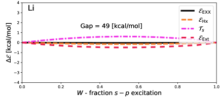
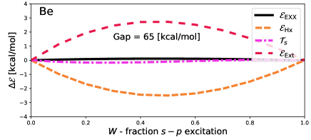
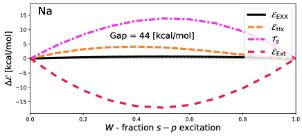
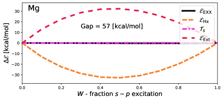
Figure 1: Non-piece-wise part ${\cal E}^{W}-[(1-W){\cal E}^{0}+W{\cal E}^{1}]$ of the energy ${\cal E}_{{\text{EXX}}}$ (solid black line) and its components ${\cal E}_{\text{Hx}}$ (orange dashes), ${\cal T}_{s}$ (magenta dashes), and ${\cal E}_{\text{Ext}}$ (red dashes), as a function of excitation weight $W$. Densities and energies obtained by self-consistent EXX calculations. Results shown for Li, Be, Na and Mg. The vertical gap ${\text{Gap}}=E_{{\text{EXX}},P_{0}}-E_{{\text{EXX}},S_{0}}$ is indicated on the plots.

The cases $W=0$ and $W=1$ are both $\mathcal{P}$-passive, and thus may be treated as ground states. In these cases, EXX gives densities,

$$n_{{\text{EXX}}}^{W=0}(r)\approx n_{S_{0}}(r), n_{{\text{EXX}}}^{W=1}(r)\approx n_{P_{0}}(r),$$ (35)

that are close to their exact counterparts in the atomic systems we consider. Consequently, we can approximately treat $n_{{\text{EXX}}}^{W=0,1}$ as the true density $n^{W=0,1}$. It then follows from ${\cal E}={\cal E}_{{\text{EXX}}}+{\cal E}_{\text{c}}$ that the energies,

$${\cal E}_{{\text{EXX}}}^{W=0}\approx E_{S_{0}}-E_{\text{c},S_{0}}^{{\text{SD}}}, {\cal E}_{{\text{EXX}}}^{W=1}\approx E_{P_{0}}-E_{\text{c},P_{0}}^{{\text{SD}}},$$ (36)

are correct up to SD correlation terms $E_{c}^{{\text{SD}}}$ and small errors from the densities. Here we neglect DD correlations at $W=0$ and $1$. In fact, there may be some DD correlations associated with (actual or effective) ground state degeneracies – we do not concern ourselves with these to focus on only the DD correlations that affect excitations directly.

For the cases $0<W<1$ the situation becomes more complicated. This is because the density $n_{{\text{EXX}}}^{W}$ that minimises Eq. (34) is not the right ensemble density, i.e.

$$n_{{\text{EXX}}}^{W}\neq{(1-W)n_{{\text{EXX}}}^{W=0}+Wn_{{\text{EXX}}}^{W=1}}\;.$$ (37)

Thus, when ${\cal E}_{{\text{EXX}}}^{W}[n_{{\text{EXX}}}^{W}]$ is employed as an estimation of the exact energy it has two sources of error:

1. It misses SD and DD correlation terms as these are not included in the EXX approximation;

2. It is not obtained at the correct density which introduces an additional source of error.

We will discuss these points further below.

First, however, we will consider how this approach affects energy terms. Figure 1 shows the deviation from piece-wise linear,

$$\Delta{\cal E}^{W}= {\cal E}^{W}-[(1-W){\cal E}^{W=0}+W{\cal E}^{W=1}].$$ (38)

of various energy quantities. Here, energies and densities are obtained approximately self-consistently, by solving the Krieger-Li-Iafrate (KLI) approximation for the self-consistent EXX potentialKrieger, Li, and Iafrate (1992). Further details of calculations are provided in Methodology.

As the goal of these self-consistent calculations is to minimise the total EEXX energy [Eq. (34)] neither energies nor densities are expected to be piece-wise linear. It is thus notable that, despite no requirement to be piece-wise linear, the EXX energy ${\cal E}_{{\text{EXX}}}$ barely deviates from piece-wise linear. Adapting arguments laid out by Gould and DobsonGould and Dobson (2013) shows that $\Delta{\cal E}_{{\text{EXX}}}^{W}$ should be concave, but says nothing about how concave it should be. In fact, a very small amount of concavity can be seen for Be and Na. In Li and Mg the concavity is invisible to the eye. In all cases it is tiny compared to deviations of other quantities.

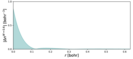
Figure 2: Difference between $n_{{\text{EXX}}}^{W}$ and piece-wise linear $n^{W}=(1-W)n_{{\text{EXX}}}^{W=0}+Wn_{{\text{EXX}}}^{W=1}$, for Mg.

Other energy deviations can be convex or concave, as they are only constrained by the fact that ${\cal E}_{{\text{EXX}}}$ must be concave. Indeed, we see substantial variations in all cases except Li. In Mg, the maximum deviation of ${\cal E}_{\text{Hx}}$ and ${\cal E}_{{\text{Ext}}}$ are more than half the vertical gap ($\text{Gap}=E_{{\text{EXX}},P_{0}}-E_{{\text{EXX}},S_{0}}$ – equivalent to the optical gap in atomic systems) in magnitude, but have equal and opposite errors which thus cancel. Figure 2 shows that the deviation of the density (Mg is shown, but other atoms are qualitatively similar) is almost exclusively found around the nucleus.

Above, we identified two sources of error found when one obtains an energy and density using (34). We can directly remove the second source (errors caused by deviation from piece-wise-linearity of densities) by using “density inversion”. That is, by seeking a potential,

$$v_{s}[n^{W}]\to n^{W}=(1-W)n^{W=0}+Wn^{W=1},$$ (39)

that yields a set of orbials $\phi_{i}[n^{W}]$ that give our target piece-wise linear density $n=\sum_{i}f_{i}|\phi_{i}|^{2}$. This lets us obtain ${\cal F}_{{\text{EXX}}}^{W}[n^{W}]$ and ${\cal E}_{{\text{EXX}}}^{W}[n^{W}]={\cal F}_{{\text{EXX}}}^{W}[n^{W}]+{\cal E}_{{\text{Ext}}}[n^{W}]>{\cal E}_{{\text{EXX}}}^{W}[n_{{\text{EXX}}}^{W}]$, and thus remove any error caused by deviations from piece-wise linearity of the density. Note, the external energy ${\cal E}_{{\text{Ext}}}[n^{W}]=\int d\boldsymbol{r}n^{W}(\boldsymbol{r})v_{{\text{Ext}}}$ is piece-wise linear, unlike ${\cal E}_{{\text{Ext}}}[n_{{\text{EXX}}}^{W}]$. Remember, in practice we approximate $n^{W=0,1}\approx n_{{\text{EXX}}}^{W=0,1}$.

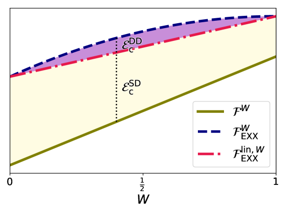
Figure 3: Qualitative illustration of ${\cal F}^{W}$ (green solid line), ${\cal F}^{\text{lin},W}_{{\text{EXX}}}$ (red dash dot line) and ${\cal F}^{W}_{{\text{EXX}}}$ (navy dashed line). Energy differences (illustrated by vertical black dotted lines) in the beige (lighter) shaded area are SD correlation energies. Those in the magenta (darker) shaded area are DD correlation energies.

In fact, we can go further than just removing contributions from densities. We can also use inversion to obtain a good approximation to the DD correlation energy contribution to the excitation energy, and thus shed light on the first identified issue. The key elements of this approach are illustrated in Figure 3

Consider the following relationships obeyed by the exact universal functional of our systems:

$${\cal F}^{W}[n^{W}]= {\cal F}_{{\text{EXX}}}^{W}[n^{W}]+{\cal E}_{\text{c}}^{W}[n^{W}]$$ (40)

$$\equiv (1-W)F_{S_{0}}[n_{S_{0}}]+WF_{P_{0}}[n_{P_{0}}]\;.$$ (41)

Next, define the linearised (lin) EXX:

$${\cal F}^{\text{lin},W}_{{\text{EXX}}}[n^{W}]= (1-W){\cal F}_{{\text{EXX}}}^{0}[n^{0}]+W{\cal F}_{{\text{EXX}}}^{1}[n^{1}]$$ (42)

$$\equiv (1-W)F_{{\text{EXX}},S_{0}}+WF_{{\text{EXX}},P_{0}}\;,$$ (43)

where $F_{{\text{EXX}},\kappa}=E_{{\text{EXX}},\kappa}-E_{{\text{Ext}},\kappa}$ for $\kappa\in S_{0},P_{0}$. We remind the reader we use $F$ rather than ${\cal F}$ to indicate that the ensembles specified by the index are treated as “pure” states. The convention can now be understood in the sense that DD correlations within (real or effective) degenerate ground-states are treated as fixed throughout the excitation. Their contributions may therefore be ignored. We introduce such an assumption for the purpose of directly focusing on the more important DD correlations in excitations.

By definition, the SD correlation terms are, $E^{{\text{SD}}}_{c,\kappa}=F^{1}[n_{\kappa}]-F_{{\text{EXX}}}[n_{\kappa}]$. It thus follows that,

$${\cal E}_{\text{c}}^{{\text{SD}},W}[n^{W}]= {\cal F}^{W}[n^{W}]-{\cal F}^{\text{lin},W}_{{{\text{EXX}}}}[n^{W}]\;,$$ (44)

$${\approx} {{\cal F}^{W}[n_{{\text{EXX}}}^{W}]-{\cal F}^{\text{lin},W}_{{\text{EXX}}}[n_{{\text{EXX}}}^{W}]\;,}$$ (45)

at least as far as excitations are concerned. This relationship is exact if we use the interacting density $n^{W}$ for $W=0,1$ or approximate if we use $n^{W}_{{\text{EXX}}}$. For arbitrary $W$ we can also write,

$${\cal F}_{{\text{EXX}}}^{W}[n^{W}]{\approx} (1-W)F_{{\text{EXX}},S_{0}}[n_{s,S_{0}}^{W}]$$

$$+WF_{{\text{EXX}},P_{0}}[n_{s,P_{0}}^{W}],$$ (46)

where $n^{W}=(1-W)n_{s,S_{0}}^{W}+Wn_{s,P_{0}}^{W}=(1-W)n_{S_{0}}+Wn_{P_{0}}$. Here, $n_{s,S_{0}}$ and $n_{s,P_{0}}$ are formed on the same set of orbitals from the KS potential $v_{s}[n^{W}]$ found by inversion of $n^{W}$. Here and henceforth, approximately equals signs indicate errors caused by treating the EXX densities for $W=0$ and $W=1$ as exact. For brevity we also drop the EXX subscript on densities $n^{W=0}$ and $n^{W=1}$.

Finally, using ${\cal E}_{\text{c}}={\cal E}_{\text{c}}^{{\text{SD}}}+{\cal E}_{\text{c}}^{{\text{DD}}}={\cal F}-{\cal F}_{{\text{EXX}}}$ and ${\cal E}_{\text{c}}^{{\text{SD}}}={\cal F}-{\cal F}^{\text{lin}}_{{\text{EXX}}}$, we obtain

$${\cal E}_{\text{c}}^{{\text{DD}},W}[n^{W}]{\approx} {\cal F}^{\text{lin},W}_{{\text{EXX}}}[n^{W}]-{\cal F}^{W}_{{\text{EXX}}}[n^{W}]\;,$$ (47)

for the DD correlation energy associated with excitations. Thus, if we calculate EXX energies at $W=0$ and $W=1$ and interpolate, this is approximately equivalent to removing SD energies at all $W$. Furthermore, deviations

$$\Delta{\cal T}_{s}^{W}{\approx} {\cal T}_{s}[n^{W}]-\{(1-W){\cal T}_{s}[n^{W=0}]+W{\cal T}_{s}[n^{W=1}]\},$$ (48)

$$\Delta{\cal E}_{\text{Hx}}^{W}{\approx} {\cal E}_{\text{Hx}}[n^{W}]-\{(1-W){\cal E}_{\text{Hx}}[n^{W=0}]+W{\cal E}_{\text{Hx}}[n^{W=1}]\},$$ (49)

have an equal and opposite component in the DD correlation terms. We are consequently able to estimate ${\cal E}_{\text{c}}^{{\text{DD}}}$ and its components without needing to know ${\cal E}_{\text{c}}^{{\text{SD}}}$ – albeit, under the assumption that $n_{{\text{EXX}}}^{W=0,1}\approx n^{W=0,1}$.

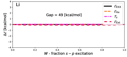
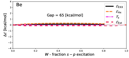
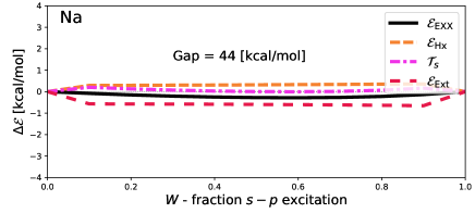
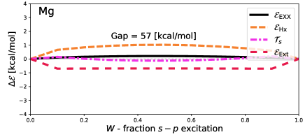
Figure 4: Like Figure 1 except the densities are found via inversion, not self-consistently. The black curve is approximately the negative of the density-driven correlation energy. The vertical gap ${\text{Gap}}=E_{{\text{EXX}},P_{0}}-E_{{\text{EXX}},S_{0}}$ is indicated on the plots.

Figure 4 reveals that the density-driven correlation energy is very small in our cases, because ${\cal E}$ barely budges from piece-wise linearity, and is well within the margin of errors ($\pm 1$ kcal/mol) from density inversion (here, estimated by considering the deviation of ${\cal E}_{{\text{Ext}}}$ which is theoretically constrained to be zero). In the case of $S$–$P$ transitions within atoms it seems that density-driven correlation energies are likely to be small. This bodes well for calculations of excitations obtained from simple EDFT approximations.

III.2 $S$–$S$ transitions and density-driven correlations

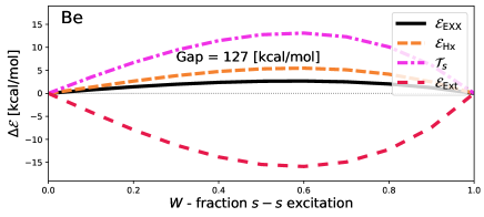
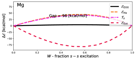
Figure 5: Like Figure 1 except showing $S$-$S$ excitations of Be and Mg. Energies and densities found self-consistently. The vertical gap ${\text{Gap}}=E_{{\text{EXX}},S_{1}}-E_{{\text{EXX}},S_{0}}$ is indicated on the plots.

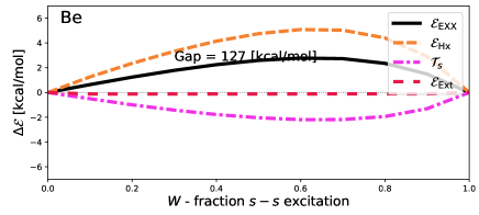
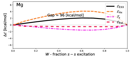
Figure 6: Like Figure 1 except showing $S$-$S$ excitations of Be and Mg. Energies and densities found by inversion. The black curve is approximately the negative of the density-driven correlation energy. The vertical gap ${\text{Gap}}=E_{{\text{EXX}},S_{1}}-E_{{\text{EXX}},S_{0}}$ is indicated on the plots.

Finally, we recognise that the $S$–$P$ transitions so far considered are not the only ones we have available by using ensembles composed of two “members”. The results of Section II.2 mean we can also study the lowest lying transition between $S$ states, as such ensembles are $\mathcal{P}$-passive.

Focusing on non-interacting states for illustration, let us detail the form of our EDMs. The full EDM is,

$$\hat{\Gamma}_{s}^{W}\equiv (1-W)\hat{\Gamma}_{s,S_{0}}+W\hat{\Gamma}_{s,S_{1}},$$ (50)

where $S_{0}$ is as before and $S_{1}$ now refers to the fact that we average over first excited states with $L=0$. Specifically, for Be, we study the excitation involving promotion of the $2s$ orbital to $3s$. $\hat{\Gamma}_{s,S_{0}}$ is defined in Eq. (26). For $S_{1}$, averaging over singlet-triplet splitting, we get,

$$\hat{\Gamma}^{\text{Be}}_{s,S_{1}}= \frac{1}{4}\sum_{\sigma,\sigma^{\prime}\in\mathord{\uparrow},\mathord{\downarrow}}|2s^{\sigma}3s^{\sigma^{\prime}}\rangle\langle 2s^{\sigma}3s^{\sigma^{\prime}}|\;.$$ (51)

For Mg we set $1s^{2}\to 1s^{2}2s^{2}$, $2s\to 3s$ and $3s\to 4s$.

Formally, the excitations we consider can only be studied for $0\leq W\leq\frac{1}{2}$. However, we found that self-consistently evaluating the fully excited state ($W=1$ – also $\frac{1}{2}<W\leq 1$) worked, despite not being formally guaranteed.

Figure 5 shows results obtained self-consistently for the $2s$–$3s$ transition in Be and the $3s$–$4s$ transition in Mg. Energies have deviations that are, compared to the total transition energy, very similar to the $S$–$P$ transition shown in Figure 1. However, the total EXX energy is noticeably more concave.

Figure 6 further highlights the concavity, and thus the importance of DD correlations. Unlike the cases shown in Figure 4, which show little deviation, the energy ${\cal E}^{W}$ deviates from piece-wise linear by up to $3$ kcal/mol for Be and $2$ kcal/mol for Mg. As discussed above, this deviation is a decent approximation to ${\cal E}_{\text{c}}^{{\text{DD}}}$, which is consequently around 2.5% of the total excitation energy of Be, and 2% of Mg. This is not a result of poor inversion either, as ${\cal E}_{{\text{Ext}}}$ shows minimal deviations from piece-wise linear.

IV Methodology

Calculations are carried out in the pyAtom Python3 code based on numpy/scipy (available on request). This code implements DFT in spherical geometries. Kohn-Sham orbitals and energies of the atoms are constructed using a spherically-symmetric and spin-unpolarised Kohn-Sham potential produced by applying the KLIKrieger, Li, and Iafrate (1992) approximation to the Greens’ function, to find the potential, $v_{\text{Hx}}(r)=\frac{\delta{\cal E}_{\text{Hx}}}{\delta n(r)}$, associated with the appropriately averaged EEXX energy, ${\cal E}_{\text{Hx}}$. Note $v_{\text{Hx}}$ is a multiplicative function of radius $r$, not a non-local operator like in Hartree-Fock theory.

The primary difference from a typical EXX DFT calculation occurs in the definition of the Hx energy. The Hx energy of a closed-shell state is, $E_{\text{Hx}}=\frac{1}{2}\sum_{ij\in\text{occ}}[4(ii|jj)-2(ij|ji)]$, written in terms of the usual Coulomb integral $(ij|kl)=\int\frac{d\boldsymbol{r}d\boldsymbol{r}^{\prime}}{|\boldsymbol{r}-\boldsymbol{r}^{\prime}|}\allowbreak\phi_{i}^{*}(\boldsymbol{r})\phi_{j}(\boldsymbol{r})\phi^{*}_{k}(\boldsymbol{r}^{\prime})\phi_{l}(\boldsymbol{r}^{\prime})$. In EEXX,

$${\cal E}_{\text{Hx}}= \frac{1}{2}\sum_{ij}\big{[}(\langle\theta_{i}\theta_{j}\rangle^{S}+\langle\theta_{i}\theta_{j}\rangle^{D})(ii|jj)-\langle\theta_{i}\theta_{j}\rangle^{S}(ij|ji)\big{]}\;,$$ (52)

has the same general form (at least in the simplified version we consider in this work restricting to single Slater determinants) but involves ensemble averaged pair-occupation factors,

$$\langle\theta_{i}\theta_{j}\rangle^{S}\equiv \sum_{\kappa}w_{\kappa}[\theta_{i\mathord{\uparrow}}^{\kappa}\theta_{j\mathord{\uparrow}}^{\kappa}+\theta_{i\mathord{\downarrow}}^{\kappa}\theta_{j\mathord{\downarrow}}^{\kappa}]\;,$$ (53)

$$\langle\theta_{i}\theta_{j}\rangle^{D}\equiv \sum_{\kappa}w_{\kappa}[\theta_{i\mathord{\uparrow}}^{\kappa}\theta_{j\mathord{\downarrow}}^{\kappa}+\theta_{i\mathord{\downarrow}}^{\kappa}\theta_{j\mathord{\uparrow}}^{\kappa}]\;,$$ (54)

for same (S) and different (D) spin pairs, respectively. Here, $\theta^{\kappa}_{i\sigma}$ is the occupation factor for orbital $i$ with spin $\sigma$ in ensemble member $\kappa$, per previous workGould and Dobson (2013); Gould et al. (2019) [see, especially, eq. 29 of Ref. Gould et al., 2019]. Eq. (52) can thus accommodate systems with even and odd numbers of electrons, and high spatial symmetriesGould and Dobson (2013).

Understanding this approach is most easily done by using an example: here, Li in its ground state. Li has a two-fold degenerate ground state which leads to a two member ensemble: $\kappa\in\{1s^{2}2s^{\mathord{\uparrow}},1s^{2}2s^{\mathord{\downarrow}}\}$. Thus, we have weights $w_{1s^{2}2s^{\mathord{\uparrow}}}=w_{1s^{2}2s^{\mathord{\downarrow}}}=\frac{1}{2}$; and occupation factors $\theta_{1s\mathord{\uparrow}}^{\kappa}=\theta_{1s\mathord{\downarrow}}^{\kappa}=1$ for $1s$ states in either ensemble member, $\kappa$, $\theta_{2s\mathord{\uparrow}}^{\kappa=1s^{2}2s^{\mathord{\uparrow}}}=\theta_{2s\mathord{\downarrow}}^{\kappa=1s^{2}2s^{\mathord{\downarrow}}}=1$ for $2s$ states, and $\theta_{i}^{\kappa}=0$ otherwise. Eqs. (53) and (54) yield $\langle\theta_{1s}\theta_{1s}\rangle^{S}=\langle\theta_{1s}\theta_{1s}\rangle^{D}=2$, $\langle\theta_{1s}\theta_{2s}\rangle^{S}=\langle\theta_{1s}\theta_{2s}\rangle^{D}=\langle\theta_{2s}\theta_{1s}\rangle^{S}=\langle\theta_{2s}\theta_{1s}\rangle^{D}=1$, $\langle\theta_{2s}\theta_{2s}\rangle^{S}=1$. The pair-occupation factor is zero otherwise. Computation of $\langle\theta_{i}\theta_{j}\rangle_{P_{0}}$ or $\langle\theta_{i}\theta_{j}\rangle_{S_{1}}$ involves changing average occupation factors and accounting for any degeneracy due to spatial symmetries. To continue our example, the $P_{0}$ state of Li (six-member ensemble of $1s^{2}2p_{m}^{\sigma}$ for $\sigma\in\{\mathord{\uparrow},\mathord{\downarrow}\}$ and $m\in\{-1,0,1\}$ with $w_{\kappa}=\frac{1}{6}$) has $\langle\theta_{1s}\theta_{1s}\rangle^{S}=\langle\theta_{1s}\theta_{1s}\rangle^{D}=2$, $\langle\theta_{1s}\theta_{2p_{m}}\rangle^{S}=\langle\theta_{1s}\theta_{2p_{m}}\rangle^{D}=\langle\theta_{2p_{m}}\theta_{1s}\rangle^{S}=\langle\theta_{2p_{m}}\theta_{1s}\rangle^{D}=\frac{1}{3}$, $\langle\theta_{2p_{m}}\theta_{2p_{m^{\prime}}}\rangle^{S}=\frac{1}{3}\delta_{mm^{\prime}}$ or zero otherwise. The $S_{1}$ state has $\langle\theta_{1s}\theta_{1s}\rangle^{S}=\langle\theta_{1s}\theta_{1s}\rangle^{D}=2$, $\langle\theta_{1s}\theta_{3s}\rangle^{S}=\langle\theta_{1s}\theta_{3s}\rangle^{D}=\langle\theta_{3s}\theta_{1s}\rangle^{S}=\langle\theta_{3s}\theta_{1s}\rangle^{D}=1$, $\langle\theta_{3s}\theta_{3s}\rangle^{S}=1$ or zero.

The work reported here then requires the additional step of averaging pair-occupation factors found for $S_{0}$ and $P_{0}$ (or for $S_{0}$ and $S_{1}$) according to the weights $W$ and $1-W$, so that

$$\langle\theta_{i}\theta_{j}\rangle^{S/D}= (1-W)\langle\theta_{i}\theta_{j}\rangle_{S_{0}}^{S/D}+W\langle\theta_{i}\theta_{j}\rangle_{P_{0}}^{S/D}\;.$$ (55)

We are thus able to obtain ${\cal E}_{\text{Hx}}$ directly, and then use it to obtain the Hx potential $v_{\text{Hx}}(r)$.

Orbitals $\phi_{i}(\boldsymbol{r})=R_{nl}(r)Y_{lm}(\hat{\boldsymbol{r}})$ are expanded into real radial parts $R_{nl}(r)$ obeying

$$\bigg{[}-\frac{\partial^{2}}{2\partial r^{2}}+\frac{l(l+1)}{2r^{2}}+v_{s}(r)\bigg{]}rR_{nl}(r)= \epsilon_{nl}rR_{nl}(r)\;,$$ (56)

and complex spherical harmonics $Y_{lm}(\hat{\boldsymbol{r}})$ (note, however, that – to the end of the overall averages considered in this work – it does not matter whether we choose single-particle orbitals with real- or complex-valued spherical harmonics). Here, $v_{s}(r)=-Z/r+v_{\text{Hx}}(r)$ is the KS potential under the EEXX approximation.

Calculations reported here used 160 radial values on a grid $r_{q}=Ax_{q}/(1-x_{q})$, where abscissae $x_{0\leq q<160}=(q+\frac{1}{2})/160$ are distributed evenly across the unit interval $(0,1)$, and $A$ is chosen based on the size of the atom involved. The Laplacian is discretised using a three-point pencil. Coulomb integrals are obtained by quadrature, using terms of form

$$u_{L;n_{1}n_{2}n_{1}^{\prime}n_{2}^{\prime}}=\sum_{ll^{\prime}}C^{L}_{ll^{\prime}}\sum_{qq^{\prime}}\omega_{q}\omega_{q^{\prime}}$$

$$~{}~{}~{}~{}\times\frac{\min[r_{q},r_{q^{\prime}}]^{L}}{\max[r_{q},r_{q^{\prime}}]^{L+1}}f_{n_{1}n_{2},l,q}f_{n_{1}^{\prime}n_{2}^{\prime},l^{\prime},q^{\prime}}\;.$$ (57)

where the sum is over allowed combinations of $l,l^{\prime}$, and $f_{n_{1}n_{2},l}(r)=R_{n_{1}l}(r)R_{n_{2}l}(r)$. Here, $\omega_{q}$ are quadrature weights and $C^{L}_{ll^{\prime}}$ are related to Clebsch-Gordon coefficients. Tests using larger grids indicate that energy differences are converged to within 0.1 kcal/mol.

The largest source of error in our calculations is thus that from density inversion, i.e. finding a potential $v^{W}\equiv v_{s}[n^{W}](r)$ so that the solutions $R_{nl}(r)$ of (56) obey $\sum_{nl}f_{nl}R_{nl}(r)^{2}=n^{W}$ [Eq. (39)], e.g., for $S$–$P$ in Be we seek to find $v^{W}$ such that $2R_{1s}^{2}+(2-W)R_{2s}^{2}+WR_{2p}^{2}=(1-W)n_{S_{0}}+Wn_{P_{0}}$. For our inversion algorithm we use the procedure outlined by Garrick et alGarrick et al. (2019).

V Conclusions

In this work we have reviewed recent advancements in ensemble density functional theory. We paid particular attention to manifolds of degenerate states, the involved symmetries, and their preservation.

Then, we introduced a method that uses exact exchange calculations to estimate density-driven correlation energies, using Kohn-Sham density inversion. This method was first demonstrated on $S$–$P$ transitions in atoms (Li, Be, Na and Mg), which revealed that density-driven correlation energies are very small in these transitions, suggesting that a naive application of ensemble DFT is acceptable for these cases provided both states are treated using spin-unpolarised orbitals obtained from ensemble calculations. Finally, by means of the same method, we investigated $S$–$S$ transition in Be and Mg. Here, the density-driven correlation energy was shown to be much more important, being up to 3 kcal/mol [Figure 6].

This is consistent with previous results on 1D moleculesGould, Kronik, and Pittalis (2018), where singlet-triplet transitions had smaller DD terms than singlet-singlet transitions. It suggests that density-driven correlations get enhanced in ensembles involving states from different energy levels but of the same symmetry type.

Applying similar studies to molecular systems is a logical next step. Also extension to periodically extended system is a very compelling step to be taken shortly. For the purpose of the present work, we simplified our task by averaging over single-triplet splittings. In actual applications, however, they will have to be resolved. Work along these lines is being pursued.

References

- Hohenberg and Kohn (1964) P. Hohenberg and W. Kohn, Phys. Rev. 136, B864 (1964).
- Kohn and Sham (1965) W. Kohn and L. J. Sham, Phys. Rev. 140, A1133 (1965).
- Matsika and Krylov (2018) S. Matsika and A. I. Krylov, Chemical Reviews 118, 6925 (2018), pMID: 30086645, https://doi.org/10.1021/acs.chemrev.8b00436 .
- Runge and Gross (1984) E. Runge and E. K. Gross, Phys. Rev. Lett. 52, 997 (1984).
- Maitra (2005) N. T. Maitra, J. Chem. Phys. 122, 234104 (2005).
- Elliott et al. (2011) P. Elliott, S. Goldson, C. Canahui, and N. T. Maitra, Chem. Phys. 391, 110 (2011).
- Maitra (2017) N. T. Maitra, J. Phys.: Cond. Matter 29, 423001 (2017).
- Baker, Scheiner, and Andzelm (1993) J. Baker, A. Scheiner, and J. Andzelm, Chem. Phys. Lett. 216, 380 (1993).
- Wittbrodt and Schlegel (1996) J. M. Wittbrodt and H. B. Schlegel, J. Chem. Phys. 105, 6574 (1996).
- Theophilou (1979) A. K. Theophilou, J. Phys. C: Solid State Phys. 12, 5419 (1979).
- Gross, Oliveira, and Kohn (1988a) E. K. U. Gross, L. N. Oliveira, and W. Kohn, Phys. Rev. A 37, 2805 (1988a).
- Gross, Oliveira, and Kohn (1988b) E. K. U. Gross, L. N. Oliveira, and W. Kohn, Phys. Rev. A 37, 2809 (1988b).
- Oliveira, Gross, and Kohn (1988) L. N. Oliveira, E. K. U. Gross, and W. Kohn, Phys. Rev. A 37, 2821 (1988).
- Valone (1980) S. M. Valone, J. Chem. Phys. 73, 4653 (1980).
- Perdew et al. (1982) J. P. Perdew, R. G. Parr, M. Levy, and J. L. Balduz, Phys. Rev. Lett. 49, 1691 (1982).
- Lieb (1983) E. H. Lieb, Int. J. Quant. Chem. 24, 243 (1983).
- Savin (1996) A. Savin, “On degeneracy, near-degeneracy and density functional theory,” (Elsevier, Amsterdam, 1996) pp. 327–358.
- Ayers (2006) P. W. Ayers, Phys. Rev. A 73, 012513 (2006).
- Gould and Pittalis (2017) T. Gould and S. Pittalis, Phys. Rev. Lett. 119, 243001 (2017).
- Gould and Pittalis (2019) T. Gould and S. Pittalis, Phys. Rev. Lett. 123, 016401 (2019).
- Senjean and Fromager (2018) B. Senjean and E. Fromager, Phys. Rev. A 98, 022513 (2018).
- Filatov and Shaik (1999) M. Filatov and S. Shaik, Chem. Phys. Lett. 304, 429 (1999).
- Franck and Fromager (2014) O. Franck and E. Fromager, Mol. Phys. 112, 1684 (2014).
- Filatov, Huix-Rotllant, and Burghardt (2015) M. Filatov, M. Huix-Rotllant, and I. Burghardt, J. Chem. Phys. 142, 184104 (2015).
- Filatov (2016) M. Filatov, “Ensemble DFT approach to excited states of strongly correlated molecular systems,” in Density-Functional Methods for Excited States, edited by N. Ferré, M. Filatov, and M. Huix-Rotllant (Springer International Publishing, Cham, 2016) pp. 97–124.
- Deur, Mazouin, and Fromager (2017) K. Deur, L. Mazouin, and E. Fromager, Phys. Rev. B 95, 035120 (2017).
- Deur and Fromager (2019) K. Deur and E. Fromager, J. Chem. Phys. 150, 094106 (2019).
- Yang et al. (2014) Z.-h. Yang, J. R. Trail, A. Pribram-Jones, K. Burke, R. J. Needs, and C. A. Ullrich, Phys. Rev. A 90, 042501 (2014).
- Pribram-Jones et al. (2014) A. Pribram-Jones, Z.-h. Yang, J. R. Trail, K. Burke, R. J. Needs, and C. A. Ullrich, J. Chem. Phys. 140, 18A541 (2014), 10.1063/1.4872255.
- Filatov (2015) M. Filatov, WIREs Comput Mol Sci 5, 146 (2015).
- Yang et al. (2017) Z.-h. Yang, A. Pribram-Jones, K. Burke, and C. A. Ullrich, Phys. Rev. Lett. 119, 033003 (2017).
- Gould, Kronik, and Pittalis (2018) T. Gould, L. Kronik, and S. Pittalis, J. Chem. Phys. 148, 174101 (2018).
- Levy (1982) M. Levy, Phys. Rev. A 26, 1200 (1982).
- Perarnau-Llobet et al. (2015) M. Perarnau-Llobet, K. V. Hovhannisyan, M. Huber, P. Skrzypczyk, N. Brunner, and A. Acín, Phys. Rev. X 5, 041011 (2015).
- Brandi, Matos, and Ferreira (1980) H. Brandi, M. D. Matos, and R. Ferreira, Chem. Phys. Lett. 73, 597 (1980).
- Gidopoulos, Papaconstantinou, and Gross (2002a) N. I. Gidopoulos, P. G. Papaconstantinou, and E. K. U. Gross, Phys. Rev. Lett. 88, 033003 (2002a).
- Pastorczak and Pernal (2014) E. Pastorczak and K. Pernal, J. Chem. Phys. 140, 18A514 (2014), https://doi.org/10.1063/1.4866998 .
- Ayers, Levy, and Nagy (2015) P. W. Ayers, M. Levy, and A. Nagy, The Journal of Chemical Physics 143, 191101 (2015), https://doi.org/10.1063/1.4934963 .
- Helgaker, Jørgensen, and Olsen (2002) T. Helgaker, P. Jørgensen, and J. Olsen, Molecular Electronic-Structure Theory (John Wiley & Sons, LTD., 2002).
- Theophilou and Gidopoulos (1995) A. K. Theophilou and N. I. Gidopoulos, Int. J. Quantum Chem. 56, 333 (1995).
- Theophilou (1997) A. K. Theophilou, Int. J. Quantum Chem. 61, 333 (1997).
- Theophilou and Papaconstantinou (2000) A. K. Theophilou and P. G. Papaconstantinou, Phys. Rev. A 61, 022502 (2000).
- Hadjisavvas and Theophilou (1985) N. Hadjisavvas and A. Theophilou, Phys. Rev. A 32, 720 (1985).
- Note (1) Recently, Fromager and coworkersDeur and Fromager (2019); Senjean and Fromager (2018) have pointed out that the flexibility of GOK can be exploited even further, in such a way to access single excited levels from calculations that need to refer only to a single ensemble-density-functional.
- Gunnarsson and Lundqvist (1976) O. Gunnarsson and B. I. Lundqvist, Phys. Rev. B 13, 4274 (1976).
- Gidopoulos, Papaconstantinou, and Gross (2002b) N. Gidopoulos, P. Papaconstantinou, and E. Gross, Physica B 318, 328 (2002b), proceedings of the 6th Patras University Euroconference on Proper ties of Condensed Matter Probed with X-ray Scattering - Electron Correla tions and Magnetism.
- Gould and Dobson (2013) T. Gould and J. F. Dobson, J. Chem. Phys. 138, 014103 (2013).
- Krieger, Li, and Iafrate (1992) J. B. Krieger, Y. Li, and G. J. Iafrate, Phys. Rev. A 45, 101 (1992).
- Gould et al. (2019) T. Gould, S. Pittalis, J. Toulouse, E. Kraisler, and L. Kronik, Phys. Chem. Chem. Phys. 21, 19805 (2019).
- Garrick et al. (2019) R. Garrick, A. Natan, T. Gould, and L. Kronik, Under review (2019), 10.26434/chemrxiv.8869460.v1.