Static Pull-in Behavior of Hybrid Levitation Micro-Actuators: Simulation, Modelling and Experimental Study

Abstract

In this article, a systematic and comprehensive approach based on finite element analysis and analytical modelling for studying static pull-in phenomena in hybrid levitation micro-actuators is presented. A finite element model of electromagnetic levitation micro-actuators based on the Lagrangian formalism is formulated and developed as a result of recent progress in the analytical calculation of mutual inductance between filament loops. In particular, the developed finite element model allows us to calculate accurately and efficiently a distribution of induced eddy current within a levitated micro-object. At the same time, this fact provides a reason for formulating the analytical model in which the distribution of the induced eddy current can be approximated by one circuit represented by a circular filament. In turn, both developed models predict the static pull-in parameters of hybrid levitation micro-actuators without needs for solving nonlinear differential equations. The results of modelling obtained by means of the developed quasi-finite element and analytical model are verified by the comparison with experimental results.

Nomenclature

${\boldsymbol{\underline{e}}^{X}}$

vector base of fixed frame {$X_{k}$}

${\boldsymbol{{e}}^{X}_{k}}$

$k$-unit vector of fixed frame {$X_{k}$} ($k=1,2,3$)

${\boldsymbol{\underline{e}}^{x}}$

vector base of coordinate frame {$x_{k}$}

${\boldsymbol{{}^{(s)}\underline{e}}^{y}}$

vector base of coordinate frame {${}^{(s)}y_{k}$} $(s=1,\ldots,n)$

${\boldsymbol{{}^{(j)}\underline{e}}^{z}}$

vector base of coordinate frame {${}^{(j)}z_{k}$} $(j=1,\ldots,N)$

$F_{l}$

generalized force ($l=1,2,3$) ($\mathrm{N}$)

${\boldsymbol{g}}$

gravity acceleration vector ($\mathrm{m}\mathrm{/}\mathrm{s}^{2}$)

$h_{l}$

height of levitation ($\mathrm{m}$)

$h$

space between the electrode surface and cm of levitated disc ($\mathrm{m}$)

$i_{cj}$

current in the $j$-wire loop $(j=1,\ldots,N)$, ($\mathrm{A}$)

$i_{s}$

current in the $s$-circular element $(s=1,\ldots,n)$ ($\mathrm{A}$)

$K$

kinetic energy ($\mathrm{J}$)

$N$

number of wire loops

$n$

number of finite elements

$L$

Lagrange function ($\mathrm{J}$)

$L_{jj}^{c}$

self-inductance of the $j$-wire loop ($\mathrm{H}$)

$L^{o}$

self-inductance of the finite circular element ($\mathrm{H}$)

$L_{ks}^{c}$

mutual inductance between $k$- and $s$-finite circular elements ($\mathrm{H}$)

$M_{kj}$

mutual inductance between the $k$-circular element and the $j$-wire loop ($\mathrm{H}$)

$m$

mass of levitated object ($\mathrm{kg}$)

$\boldsymbol{q}$

translational position vector of levitated object ($\mathrm{m}$)

$R$

electrical resistance of finite element ($\mathrm{\SIUnitSymbolOhm}$)

$R_{e}$

radius of finite element ($\mathrm{m}$)

$R_{cj}$

radius of j-circular coil filament ($\mathrm{m}$)

${}^{(j)}\boldsymbol{r}_{c}$

linear position vector of $j$-wire loop ($\mathrm{m}$)

$\boldsymbol{r}_{cm}$

linear position vector of centre of mass of levitated object ($\mathrm{m}$)

$T_{l}$

generalized torque ($l=1,2,3$) ($\mathrm{N}\text{\,}\mathrm{m}$)

$W_{m}$

energy stored within electromagnetic field ($\mathrm{J}$)

{$X_{k}$}

fixed frame ($k=1,2,3$)

{$x_{k}$}

coordinate frame attached to levitated object ($k=1,2,3$)

{${}^{(s)}y_{k}$}

coordinate frame attached to $s$-finite element ($k=1,2,3$)

{${}^{(j)}z_{k}$}

coordinate frame attached to $j$-wire loop ($k=1,2,3$)

Greek symbols

$\beta$

dimensionless square voltage

$\kappa$

dimensionless parameter $h/h_{l}$

$\lambda$

dimensionless displacement $q_{3}/h$

$\mu_{l}$

damping coefficient ($l=1,2,3$) ($\mathrm{N}\text{\,}\mathrm{s}\text{\,}{\mathrm{m}}^{-1}$)

$\nu_{l}$

damping coefficient ($l=1,2,3$) ($\mathrm{N}\text{\,}\mathrm{s}\text{\,}{\mathrm{rad}}^{-1}$)

$\xi$

dimensionless parameter $h_{l}/(2R_{l})$

$\Pi$

potential energy ($\mathrm{J}$)

${}^{(s)}\boldsymbol{\rho}$

vector of linear position of $s$-circular element in vector base ${\boldsymbol{\underline{e}}^{x}}$ ($\mathrm{m}$)

$\Psi$

dissipation energy ($\mathrm{J}\text{\,}{\mathrm{s}}^{-1}$)

${}^{(s)}\boldsymbol{\phi}$

vector of angular position of $s$-circular element (Brayn angles) ($\mathrm{rad}$)

${}^{(j)}\boldsymbol{\phi}_{c}$

vector of angular position of $j$-wire loop (Brayn angles) ($\mathrm{rad}$)

$\boldsymbol{\varphi}$

angular position vector of levitated object ($\mathrm{rad}$)

$\boldsymbol{\omega}$

vector of angular velocity of levitated object ($\mathrm{rad}\text{\,}{\mathrm{s}}^{-1}$)

Subscripts

cm

centre of mass

DLMA

diamagnetic levitation micro-actuators

ELMA

electric levitation micro-actuators

FEM

finite element model

HLMA

hybrid levitation micro-actuators

ILMA

inductive levitation micro-actuators

MLMA

magnetic levitation micro-actuators

I Introduction

Electromagnetic levitation micro-actuators employing remote ponderomotive forces, in order to act on a target environment or simply compensate a gravity force for holding stably a micro-object at the equilibrium without mechanical attachment, have already found wide applications and demonstrated a new generation of micro-sensors and -actuators with increased operational capabilities and overcoming the domination of friction over inertial forces at the micro-scale [1].

There are a number of techniques, which provide the implementation of electromagnetic levitation into a micro-actuator system and can be classified according to using materials and the sources of the force fields as follows: electric levitation (ELMA), magnetic levitation (MLMA) and hybrid levitation micro-actuators (HLMA). In particular, ELMA were successfully used as linear transporters [2] and in micro-inertial sensors [3, 4, 5]. MLAM can be further split into inductive (ILMA), diamagnetic (DLMA) and superconducting micro-actuators, which have found applications in micro-bearings [6, 7, 8], micro-mirrors [9, 10], micro-gyroscopes [11, 12], micro-accelerometers [13], bistable switches [14] and nano-force sensors [15].

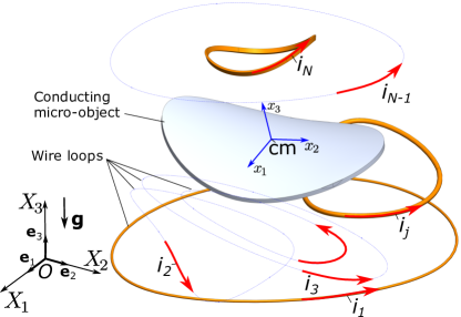
Figure 1: The generalized scheme of electromagnetic levitation system, in which a conducting micro-object is levitated by a system of arbitrary shaped wire-loops with ac currents: $X_{1}X_{2}X_{3}$ is the fixed coordinate frame with the corresponding unit vectors $\boldsymbol{e}_{1}$, $\boldsymbol{e}_{2}$, and $\boldsymbol{e}_{3}$, respectively; g is the gravity acceleration vector directed along the $X_{3}$-axis; $x_{1}x_{2}x_{3}$ is the coordinate frame assigned to object principal axes with the origin at its centre of mass (cm); $i_{j}$ is the current in the $j$-wire loop.

In HLMA different force fields are combined, for instance, magneto- and electro-static, variable magnetic and electro-static or magneto-static and variable magnetic fields, which make the main difference of HLMA from both ELAM and MLMA. In particular, capabilities of HLMA were demonstrated in applications as micro-motors [16, 17] and micro-accelerators [18]. A wide range of different operation modes such as the linear and angular positioning, bistable linear and angular actuations and the adjustment of stiffness components of a levitated micro-disc were demonstrated and experimentally studied in the prototype reported in [19]. In this prototype, the stiffness components were adjusted by changing an equilibrium position of the inductively levitated disc along the vertical axis. Recently, the novel HLMA, in which the electrostatic forces acting on the bottom and top surfaces of the inductively levitated micro-disc keep its equilibrium position and at the same time decrease a vertical component of stiffness by means of increasing the strength of electrostatic field, was presented in [20, 21]. A concept of this actuator for an application as a linear micro-accelerometer was proposed in [22]. Thus, HLMA establish a promising direction for further improvement in the performance of micro-sensors and -actuators.

As seen, the electrostatic actuation is one of the main principles applied in HLMA to a passively levitated micro-object (proof mass) for the adjustment of their static and dynamic characteristics. Simultaneously, electrostatic forces acting on the levitating micro-object restrict its range of stable motion by pull-in instability. Moreover, due to the fact that the spring constant created by a magnetic contactless suspension of HLMA has a nonlinear dependence on displacements, hence the pull-in phenomenon in HLMA cannot be described and characterized by the classic pull-in effect occurring in the spring-mass system with electrostatic actuation [23].

Another obstacle for analysing HLMA arises due to the fact that the description of electromagnetic levitation requires the application of the Maxwell equations. Although, these equations are universally applicable, but their application even for simple designs is extremely difficult task [24]. Even these designs are studied numerically by using commercially available software, this task is still a challenge [25, 26, 27, 28], which is not able to cover all aspects including stability or stable levitation and nonlinear dynamical response [29].

Figure 2: The conducting micro-object is meshed by finite elements of circular shape: $\{^{(s)}y_{l}\}$ and $\{^{(k)}y_{l}\}$ ($l=1,2,3$) are the coordinate frames assigned to s- and k- circular element, respectively.

In this work, in order to avoid having a deal with field equations, the quasi-finite element model (quasi-FEM) of HLMA based on the Lagrangian formalism is developed. The mathematical formulation of this developed quasi-FEM becomes possible due to the recent progress in analytical calculation of mutual inductance between filament loops [30, 31] and the technique proposed in [32], which was then generalized in [33, 34], where the induced eddy current into a levitated micro-object is considered as a finite collection of $m$-eddy current circuits. The quasi-FEM helps us to support the mathematical reasoning of applicability of analytical modeling for, in particular, in axially symmetric designs of HLMA to study static pull-in instability. Although, the analytical model has some restrictions in application because of made assumptions in comparing with the quasi-FEM, which is universally applicable. However, arising some particular cases, discussing in this work, due to designs of HLMA can be very accurately treated by the analytical model presenting a solution in simple analytical forms, which are convenient and very efficient for the practical application. The general advantage of both models is that they predict the static pull-in parameters of HLMA without needs for solving nonlinear differential equations. The results of modeling obtained by means of the developed quasi-finite element and analytical model are verified by the comparison with experimental results.

II Quasi-finite element model

Let us consider a general design configuration of an electromagnetic levitation system as shown in Fig. 1, which consists of $N$-arbitrary shaped wire loops and a levitated cunducting object. Each $j$-th wire loop is fed by its own ac current denoted by $i_{cj}$ with the index corresponding to the index of the wire loop. The set of wire loops generates the alternating magnetic flux passing through the levitated object. In turn, the eddy current is induced within the conducting object. Force interaction between induced eddy current and currents in wire loops provides the compensation of the gravity force acting on the conducting object along $X_{3}$-axis of an inertial frame {$X_{k}$} ($k=1,2,3$) and levitates then it sably at an equilibrium position. Assuming that the levitated object is a rigid body, then its equilibrium position can be defined through the six generalized coordinates corresponding to the three translation coordinates and three angular ones with respect to the fixed frame {$X_{k}$} ($k=1,2,3$) with the vector base ${\boldsymbol{\underline{e}}^{X}}=[\boldsymbol{e}^{X}_{1},\boldsymbol{e}^{X}_{2},\boldsymbol{e}^{X}_{3}]^{T}$, where $\boldsymbol{e}^{X}_{k}$ ($k=1,2,3$) are unit vectors of ${\boldsymbol{\underline{e}}^{X}}$. (The notations are adopted from the book of J. Wittenburg [35], which provide clearly distinguish between a vector, a base, and a matrix).

In order to specify these six generalized coordinates, the coordinate frame {$x_{k}$} ($k=1,2,3$) with the base ${\boldsymbol{\underline{e}}^{x}}$ and corresponding unit vectors $\boldsymbol{{e}}^{x}_{k}$ ($k=1,2,3$) is rigidly attached to the levitated object, in such a way, that its origin is located at the centre of mass of the object as shown in Fig. 1. Also, axes of the coordinate frame {$x_{k}$} ($k=1,2,3$) coincide with principal axes of inertia of the micro-object. The translational position of the micro-object cm with respect to the fixed frame is characterized by the vector $\boldsymbol{q}=[q_{1},q_{2},q_{3}]^{T}$ and the angular one by the Brayn angles (Cardan angles) denoted as $\varphi_{k}$ ($k=1,2,3$). Thus, both vectors, namely, $\boldsymbol{q}$ and $\boldsymbol{\varphi}$ can be considered as independent generalized coordinates of mechanical part of the electromagnetic levitation system.

Now let us assume that the condition of quasistationarity is hold [36, page 7], [37, page 493], hence induced eddy current within the micro-object can be represented by $n$-electric circuits (finite elements), each of them consists of the inductor and resistor connecting in series [34]. Meshing the levitated micro-object by $n$-elements having the circle shape of the same radius as shown in Fig. 2, we denote $i_{k}$ $(k=1,2,\ldots,n)$ as the induced eddy current corresponding to the $k$-element, which can be represented as the generalized velocities of electromagnetic part of the levitation system. The linear position of $s$-circular element with respect to the coordinate frame {$x_{k}$} ($k=1,2,3$) is defined by the vector ${}^{(s)}\boldsymbol{\rho}$, but the angular position of the same element is determined by Brayn angles, namely, ${}^{(s)}\boldsymbol{\phi}=[^{(s)}\phi_{1},^{(s)}\phi_{2},0]^{T}$.

Adapting the generalized coordinates and the assumptions introduced above, the model can be written by using the Lagrange - Maxwell equations as follows

$$\left\{\begin{array}[]{l}{\displaystyle{\frac{d}{dt}\left(\frac{\partial L}{\partial i_{k}}\right)+\frac{\partial\Psi}{\partial i_{k}}=0;\;k=1,\ldots,n};}\\ {\displaystyle{\frac{d}{dt}\left(\frac{\partial L}{\partial\dot{q_{l}}}\right)-\frac{\partial L}{\partial q_{l}}+\frac{\partial\Psi}{\partial\dot{q_{l}}}=F_{l};\;l=1,2,3;}}\\ {\displaystyle{\frac{d}{dt}\left(\frac{\partial L}{\partial\dot{\varphi_{l}}}\right)-\frac{\partial L}{\partial\varphi_{l}}+\frac{\partial\Psi}{\partial\dot{\varphi_{l}}}=T_{l};\;l=1,2,3,}}\\ \end{array}\right.$$ (1)

where $L=K-\Pi+W_{m}$ is the Lagrange function for the micro-object-coil system; $K=K(\dot{\boldsymbol{q}},\dot{\boldsymbol{\varphi}})$ is the kinetic energy of the system; $\Pi=\Pi({\boldsymbol{q}},{\boldsymbol{\varphi}})$ is the potential energy of the system; $W_{m}=W_{m}({\boldsymbol{q}},{\boldsymbol{\varphi}},i_{c1},\ldots,i_{cN},i_{1},\ldots,i_{n})$ is the energy stored in the electromagnetic field; $\Psi=\Psi(\dot{\boldsymbol{q}},\dot{\boldsymbol{\varphi}},i_{1},\ldots,i_{n})$ is the dissipation function; $F_{l}$ and $T_{l}$ ($l=1,2,3$) are the generalized forces and torques, respectively, acting on the micro-object relative to the appropriate generalized coordinates.

The kinetic energy is

$${\displaystyle K=\frac{1}{2}\sum_{l=1}^{3}m{\dot{q}_{l}}^{2}+\frac{1}{2}\sum_{l=1}^{3}J_{l}{\dot{\omega}_{l}}^{2}},$$ (2)

where $m$ is the mass of the micro-object; $J_{l}$ ($l=1,2,3$) are principal moments of inertia of the micro-object; $\omega_{l}=\omega_{l}({\boldsymbol{\varphi}},\dot{\boldsymbol{\varphi}})$ ($l=1,2,3$) are the components of the vector $\boldsymbol{\omega}$ of angular velocity of the micro-object relative to the fixed coordinate frame.

According to Fig. 1, the potential energy can be defined simply as follows

$$\Pi=mgq_{3}.$$ (3)

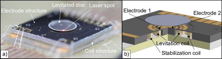
Figure 3: Experimental test of pull-in actuation in the hybrid levitation micro-actuator [19]: a) stable levitation of the disc having a diameter of 2.8 mm; b) 3D model of the device shows the location of coils and energized electrodes 1 and 2 to perform the pull-in actuation of the levitated disc.

The dissipation function is

$${\displaystyle\Psi=\frac{1}{2}\sum_{l=1}^{3}\mu_{l}{\dot{q}_{l}}^{2}+\frac{1}{2}\sum_{l=1}^{3}\nu_{l}{\dot{\varphi}_{l}}^{2}+\frac{1}{2}R\sum_{k=1}^{n}i_{k}^{2},}$$ (4)

where $\mu_{l}$ and $\nu_{l}$ ($l=1,2,3$) are the damping coefficients; $R$ is the electrical resistance of the element. The energy stored within the electromagnetic field can be written as

$$\begin{split}{\displaystyle W_{m}=\frac{1}{2}\sum_{j=1}^{N}\sum_{s=1}^{N}L_{js}^{c}i_{cj}i_{cs}+\frac{1}{2}\sum_{k=1}^{n}\sum_{s=1}^{n}L_{ks}^{o}i_{k}i_{s}}\\ {\displaystyle+\sum_{k=1}^{n}\sum_{j=1}^{N}M_{kj}i_{k}i_{cj}},\end{split}$$ (5)

where $L_{jj}^{c}$ is the self-inductance of the $j$-wire loop; $L_{js}^{c}$, $j\neq s$ is the mutual inductance between $j$- and $s$-coils; $L_{kk}^{o}=L^{o}$ is the self-inductance of the circular element; $L_{ks}^{o}=L_{ks}^{o}({{}^{(k,s)}\boldsymbol{\rho}},{{}^{(k,s)}\boldsymbol{\phi}})$, $k\neq s$ is the mutual inductance between $k$- and $s$-finite circular elements (besides, ${}^{(k,s)}\boldsymbol{\rho}={{}^{(k)}\boldsymbol{\rho}}-{{}^{(s)}\boldsymbol{\rho}}$ and ${}^{(k,s)}\boldsymbol{\phi}={{}^{(k)}\boldsymbol{\phi}}-{{}^{(s)}\boldsymbol{\phi}}$, see Fig. 2); $M_{kj}=M_{kj}({\boldsymbol{q}},{\boldsymbol{\varphi}})$ is the mutual inductance between the $k$-circular element and the $j$-wire loop.

As it was shown in works [38, 34] upon assuming quasi-static behavior of the micro-object, the induced eddy currents $i_{k}$ ($k=1,\ldots,n$) in circular elements can be directly expressed in terms of coil currents $i_{cj}(j=1,\ldots,N)$. Also, assuming that for each coil, the current $i_{cj}$ is a periodic signal with an amplitude of $I_{cj}$ (in general the amplitude is assumed to be a complex value) at the same frequency $f$, we can write $i_{cj}=I_{cj}e^{\jmath ft},$ where $\jmath=\sqrt{-1}$. Then, the $k-$ eddy current can be represented as $i_{k}=I_{k}e^{\jmath ft},$ where $I_{k}$ is the amplitude. Hence, according to [38, 34] first $n$ equations of set (1) can be solved and the induced eddy current per circular element becomes a solution of the following set of linear equations

$$\begin{array}[]{l}{\displaystyle{\left[L^{o}+R/(\jmath f)\right]I_{k}+\sum_{s=1,\;s\neq k}^{n}L_{ks}^{o}I_{s}=-\sum_{j=1}^{N}M_{kj}I_{cj};}}\\ k=1,\ldots,n.\end{array}$$ (6)

Combining the set (6) with the last six equations of (1) the quasi-finite element model of inductive levitation system is obtained. Thus, the obtained quasi-FEM is the combination of finite element manner to calculate induced eddy current and the set of six differential equations describing the behavior of mechanical part of electromagnetic levitation system.

Based on the proposed quasi-FEM the following procedure for the analysis and study of induction levitation micro-systems can be suggested. At the beginning, the levitated micro-object is meshed by circular elements of the same radius, $R_{e}$, as shown in Fig. 2, a value of which is defined by a number of elements, $n$. The result of meshing becomes a list of elements $\{^{(s)}\boldsymbol{\underline{C}}=[^{(s)}\boldsymbol{\rho},^{(s)}\boldsymbol{\phi}]^{T}\}$ ($s=1,\ldots,n$) containing information about a radius vector and an angular orientation for each element with respect to the coordinate frame {$x_{k}$} ($k=1,2,3$). Now a matrix corresponding to the left side of equation (6) can be formed as follows

$$\underline{L}=\left[L^{o}+R/(\jmath f)\right]\underline{E}+\underline{M}^{o},$$ (7)

where $\underline{E}$ is the $(n\times n)$ unit matrix, $\underline{M}^{o}$ is the $(n\times n)$ -symmetric hollow matrix whose elements are $L_{ks}^{o}$ ($k\neq s$). The self-inductance of the circular element is calculated by the known formula for a circular ring of circular cross-section

$$L^{o}=\mu_{0}R_{e}\left[\ln 8/\varepsilon-7/4+\varepsilon^{2}/8\left(\ln 8/\varepsilon+1/3\right)\right],$$ (8)

where $\mu_{0}$ is the magnetic permeability of free space, $\varepsilon=th/(2R_{e})$, $th$ is the thickness of a mashed layer of micro-object. It is recommended that the parameter $\varepsilon$ is selected to be not larger 0.1. Elements of the $\underline{M}^{o}$ matrix, $L_{ks}^{o}$ ($k\neq s$) can be calculated by the formulas developed in works [30, 31]. Using the list of elements $\{^{(s)}\boldsymbol{\underline{C}}\}$, we can estimate $L_{ks}^{o}$ as follows $L_{ks}^{o}=L_{ks}^{o}\left({}^{(k,s)}\boldsymbol{\underline{C}}\right)$, where ${}^{(k,s)}\boldsymbol{\underline{C}}=^{(k)}\boldsymbol{\underline{C}}-^{(s)}\boldsymbol{\underline{C}}$.

Then, we assign to each coil the coordinate frame {${}^{(j)}z_{k}$} ($k=1,2,3$) with the corresponding base ${}^{(j)}\boldsymbol{\underline{e}}^{z}$. The linear and angular position of {${}^{(j)}z_{k}$} ($k=1,2,3$) with respect to the fixed frame {$X_{k}$} ($k=1,2,3$) is defined by the radius vector ${}^{(j)}\boldsymbol{{r}_{c}^{X}}$ and the Brayn angles ${}^{(j)}\boldsymbol{\phi_{c}}$ $(j=1,\ldots,N)$, respectively. Knowing a projection of the $j$-coil filament loop on the ${}^{(k)}y_{1}$-${}^{(k)}y_{2}$ plane of the $k$- circular element, the Kalantarov-Zeitlin method [31] can be used in order to calculate the mutual inductance. Hence, the $(n\times N)$ matrix $\underline{M}_{c}$ consisting of elements of the mutual inductance $M_{kj}$ can be obtained. The induced eddy current in each circular element is a solution of the following matrix equation

$$\underline{I}=\underline{L}^{-1}\underline{M}_{c}\underline{I}_{c},$$ (9)

where $\underline{I}$ is the $(n\times 1)$ matrix of eddy currents and $\underline{I}_{c}=[I_{c1}I_{c2}\ldots I_{cN}]^{T}$ is the given $(N\times 1)$ matrix of currents in coils.

Finally, substituting the eddy current $\underline{I}$ into the stored electromagnetic energy (5) the ponderomotive forces acting on the levitated object can be found as the first derivative of the stored electromagnetic energy with respect to the generalized coordinates of mechanical part. Thus, in a matrix form we can write as

$$\begin{array}[]{l}{\displaystyle{F_{l}=\frac{\partial W_{m}}{\partial q_{l}}=\underline{I}^{T}\frac{\partial\underline{M}_{c}}{\partial q_{l}}\underline{I}_{c};\;l=1,2,3;}}\\ {\displaystyle{T_{l}=\frac{\partial W_{m}}{\partial\varphi_{l}}=\underline{I}^{T}\frac{\partial\underline{M}_{c}}{\partial\varphi_{l}}\underline{I}_{c};\;l=1,2,3.}}\\ \end{array}$$ (10)

III Hybrid Levitation Micro-actuators

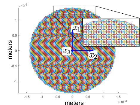
Figure 4: Disc of a diameter of $2.8\text{\,}\mathrm{mm}$ is meshed by 3993 circular elements.

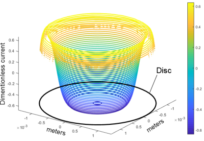
Figure 5: The distribution of the eddy current in mesh circular elements.

Let us consider one of the designs of hybrid levitation micro-actuators base on the two coil structure for stable levitation and electrode structure to generate electrostatic force acting on the bottom surface of the levitated micro-disc. In particular, such the design was implemented into the prototype of HLMA, which is shown in Fig. 3a) and was studied experimentally in works [19, 39]. Two coaxial solenoidal microcoils of the coil structure was fabricated on the pyrex substrate and were excited by ac current having a frequency of 10 MHz. The diameters of the two coils shown in Fig. 3b), namely, levitation and stabilization one were $2000\text{\,}\mathrm{\SIUnitSymbolMicro m}3800\text{\,}\mathrm{\SIUnitSymbolMicro m}$, respectively. The inner (levitation) coil had 20 windings and the outer (stabilisation) coil had 12 windings of a gold wire with a diameter of $25\text{\,}\mathrm{\SIUnitSymbolMicro m}$. The coil structure was covered by the electrode structure fabricated on a Si wafer. According to the design, the electrodes were located above the coil post at a height of $25\text{\,}\mathrm{\SIUnitSymbolMicro m}$. In order to carry out the pull-in actuation of the disc, electrodes 1 and 2, having the same area, $A_{e}$, of $8.0\cdot 10^{-7}$ m² as shown in Fig. 3b), were energized in a way that the disc was moved toward the electrode surface. The detailed results of the experimental studies and measurements of the pull-in actuation such as the pull-in voltage and displacement had been presented and discussed in [19, 39]. In this paper, the pull-in mechanism in the considered design of HLMA is comprehensively studying theoretically by means of analytical modelling and numerical simulation based on the developed quasi-FEM.

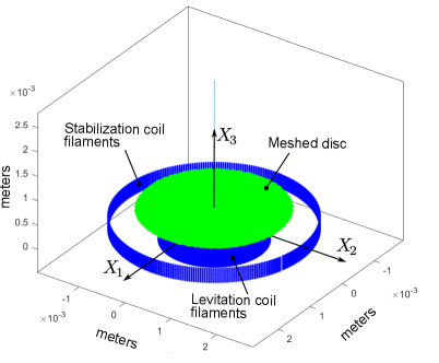
Figure 6: 3D geometrical scheme of HLMA for eddy current simulation: {$X_{k}$} ($k=1,2,3$) is the fixed coordinate frame.

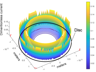
Figure 7: The distribution of magnitudes of eddy current with respect to unit vectors of $\boldsymbol{{e}}^{x}_{1}$ and $\boldsymbol{{e}}^{x}_{2}$ of the base ${\boldsymbol{\underline{e}}^{x}}$.

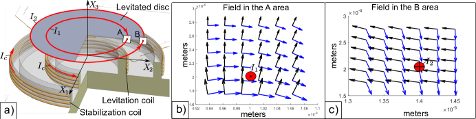
Figure 8: Modelling of linear pull-in actuation: a) scheme of HLMA based on the approximation of induced eddy current in the disc by two eddy current circuits with $I_{1}$ and $I_{2}$ currents corresponding to its maximum magnitudes; b) the map of magnetic field (blue arrows) and its corresponded gradient (black arrows) within the A area build on the $X_{3}$-$X_{2}$ plane around the $I_{1}$ circuit (see Fig. 8a)); c) the map of magnetic field and its corresponded gradient within the B area build on the $X_{3}$-$X_{2}$ plane around the $I_{2}$ circuit (see Fig. 8a)).

IV Eddy current simulation

In this section a distribution of induced eddy current within a disc having a diameter of $2.8\text{\,}\mathrm{mm}$ levitated at height, $h_{l}$, of $200\text{\,}\mathrm{\SIUnitSymbolMicro m}$ by the coil structure corresponding to the design of HLMA described above in Sec. III is simulated by the developed quasi-FEM. According to the proposed procedure, the disc is homogenously meshed by 3993 circular elements. A result of meshing is a map of the location of elements with respect to the coordinate frame {$x_{k}$} ($k=1,2,3$), the origin of which is placed at the centre of the disc, as shown in Fig 4. Each element crosses its neighboring element only at one point. Depending on the location of neighboring element at the top, right, bottom and left side, this point can be placed on the element perimeter at an angle of $0\text{\,}\mathrm{\SIUnitSymbolDegree}90\text{\,}\mathrm{\SIUnitSymbolDegree}180\text{\,}\mathrm{\SIUnitSymbolDegree}270\text{\,}\mathrm{\SIUnitSymbolDegree}$ subtended at the center of the circular element, respectively. Elements are numbering from left to right in each line. Because of the plane shape of the levitated micro-object, vectors of the list of elements $\{^{(s)}\boldsymbol{\underline{C}}\}$ have the following structures, namely, ${}^{(s)}\boldsymbol{\rho}=[^{(s)}x_{1},^{(s)}x_{2},0]^{T}$ and ${}^{(s)}\boldsymbol{\phi}=[0,0,0]^{T}$ ($s=1,\ldots,n$). Knowing $\{^{(s)}\boldsymbol{\underline{C}}\}$, the $\underline{L}$ matrix can be calculated by Eq. (7).

3D geometry of two micro-coils is approximated by a series of circular filaments. Hence, depending on the number of windings, the levitation coil is replaced by 20 circular filaments, while the stabilization coil by 12 circular filaments. Thus, the total number of circular filaments, $N$, is 32. Assigning the origin of the fixed frame {$X_{k}$} ($k=1,2,3$) to the centre of the circular filament corresponding to the first top winding of the levitation coil, the linear position of the circular filaments of levitation coil can be defined as ${}^{(j)}\boldsymbol{{r}_{c}}=[0,0,(j-1)\cdot p]^{T}$, $(j=1,\ldots,20)$, where $p$ is the pitch equaling to $25\text{\,}\mathrm{\SIUnitSymbolMicro m}$. The same is applicable for stabilization coil, ${}^{(j)}\boldsymbol{{r}_{c}}=[0,0,(j-21)\cdot p]^{T}$, with the difference that the index $j$ is varied from 21 by 32. For both coils, the Brayn angle of each circular filament is ${}^{(j)}\boldsymbol{\phi_{c}}=[0,0,0]^{T}$, $(j=1,\ldots,32)$. Accounting for the values of diameters of levitation and stabilization coils, 3D geometrical scheme of HLMA for eddy current simulation can be build as shown in Fig. 6.

The position of the coordinate frame {$x_{k}$} ($k=1,2,3$) with respect to the fixed frame {$X_{k}$} ($k=1,2,3$) is defined by the radius vector $\boldsymbol{{r}}_{cm}=[0,0,h_{l}]^{T}$. Then, the position of the $s$-mesh element with respect to the coordinate frame {${}^{(j)}z_{k}$} ($k=1,2,3$) assigned to the $j$-coil filament can be found as ${}^{(s,j)}\boldsymbol{{r}}=\boldsymbol{{r}}_{cm}+{{}^{(s)}\boldsymbol{\rho}}-{{}^{(j)}\boldsymbol{{r}}}_{c}$ or in a matrix form as

$$^{(s,j)}\underline{{r}}^{z}={{}^{(j)}\underline{A}^{zX}}{\underline{r}}_{cm}^{X}+{{}^{(j)}\underline{A}}^{zx}{{}^{(s)}\underline{\rho}^{x}}-^{(j)}\underline{A}^{zX}{{}^{(j)}\underline{{r}}_{c}^{X}},$$ (11)

where ${}^{(j)}\underline{A}^{zX}={{}^{(j)}\underline{A}^{zX}}\left({{}^{(j)}\boldsymbol{\phi_{c}}}\right)={{}^{(j)}\boldsymbol{\underline{e}}^{z}}\cdot{\boldsymbol{\underline{e}}^{X}}$ and ${}^{(j)}\underline{A}^{zx}={{}^{(j)}\underline{A}^{zX}}\left({{}^{(j)}\boldsymbol{\phi_{c}}}\right)\underline{A}^{Xx}(\boldsymbol{\varphi})={{}^{(j)}\boldsymbol{\underline{e}}^{z}}\cdot{\boldsymbol{\underline{e}}^{x}}$ are the direction cosine matrices. Because all angles are zero, hence ${}^{(j)}\underline{A}^{zx}={{}^{(j)}\underline{A}^{zX}}=\underline{E}$, where $\underline{E}$ is the ($3\times 3$) unit matrix. Since the coils are represented by the circular filaments and using the radius vector ${}^{(s,j)}\boldsymbol{{r}}$, the mutual inductance between the $j$- coil and $s$-meshed element can be calculated directly by the formula presented in [31]. Thereby, the $\underline{M}_{c}$ matrix can be formed. It is convenient to present the result of calculation in the dimensionless form. For this reason, the dimensionless currents in the levitation coil and stabilization one are introduced by dividing currents on the amplitude of the current in the levitation coil. Since the amplitudes of the current in both coil are the same. Hence, the input current in the levitation coil filaments are to be one, while in the stabilization coil filaments to be minus one. Now, the induced eddy current in dimensionless values can be calculated by Eq. (9).

In order to illustratively present the calculation result, the obtained ($3993\times 1$) eddy current matrix, $\underline{I}$, is transformed into the ($71\times 71$) 2D matrix, $\underline{I}$. Data in this ($71\times 71$) 2D matrix are allocated similarly to the structure corresponding to Fig. 4. Then, the distribution along the disc surface of induced eddy current in mesh circular elements are shown in Fig. 5. The analysis of Fig. 5 shows that in a central area of the disc, corresponding to the area of the circular cross-section of the levitation coil, the eddy current has the negative sign (it means that the direction of induced eddy current flow is opposite to the flow direction in the levitation coil) due to the significant contribution of the ac magnetic field generated by this coil. While, outside of this area, a sign becomes positive due to the ac magnetic field of the stabilization coil.

Now let us present the obtained result in the vector form through unit vectors $\boldsymbol{{e}}^{x}_{1}$ and $\boldsymbol{{e}}^{x}_{2}$ of the base ${\boldsymbol{\underline{e}}^{x}}$. Taking the numerical gradient of the ($71\times 71$) 2D matrix, $\underline{I}$ with respect to the rows and columns, the components in the form of the ($71\times 71$) 2D matrixs of $\underline{I}_{1}$ and $\underline{I}_{2}$ relative to the unit vectors $\boldsymbol{{e}}^{x}_{1}$ and $\boldsymbol{{e}}^{x}_{2}$ are calculated, respectively. Then, the ($71\times 71$) 2D matrix of magnitudes of the eddy current for each mesh point is estimated by $\sqrt{{\underline{I}_{1}}^{2}+{\underline{I}_{2}}^{2}}$. The result of estimation is shown in Fig. 7. Fig. 7 depicts that maximum magnitudes of eddy current are concentrated along the edge of the disc and in its central part along the circle having the same diameter as the levitation coil. This result is similar to one obtained by Lu in work [28], where the induced eddy current in a disc levitated by two coils with the similar design was simulated by COMSOL software. Both results provide the reason and applicability of the approximation based on a two eddy current circuits, for the analysis of HLMAs with an axially symmetric design, which was proposed in [34] and successfully used for the study of their stability and dynamics.

V Analytical model of static linear pull-in actuation

In this section, the approximation of induced eddy current within the disc based on two eddy current circuits is applied to model the linear pull-in actuation in HLMA with the design under consideration. Scheme for modelling is shown in Fig. 8a). Due to particularities of the HLMA design, a radius of the $I_{1}$ circuit is equal to $1\text{\,}\mathrm{mm}$, while a radius of the $I_{2}$ circuit is restricted by the radius of disc equaling to $1.4\text{\,}\mathrm{mm}$. Let us examine the field distribution around these two circles of eddy current circuits. Since the design is axially symmetric, it is enough to consider some areas such as denoted by $A$ and $B$ as shown in Fig. 8a) cutting, for instance, on the $X_{3}$-$X_{2}$ plane and crossing the $I_{1}$ and $I_{2}$ circuit, respectively. Mapping the field in the $A$ and $B$ area shows that the force acting on the $I_{1}$ circuit determined by the corresponded gradient of the field is directed vertically and lifts up the disc, while the force acting on the $I_{2}$ circuit has almost horizontal direction and pushes the disc toward the center as presented in Fig.8b) and c), respectively. Noting that the names of coils as levitation and stabilization coil reflect their functionalities coming form the field analysis conducted above. It can be assumed that for a diameter of disc equaling to $2.8\text{\,}\mathrm{mm}$ the influence of the $I_{2}$ circuit on the linear pull-in actuation is small and can be neglected. Thus, modelling of the linear pull-in actuation is reduced to the force interaction between the currents in the levitation coil and the $I_{1}$ circuit.

Then, the behavior of the disc along the $X_{3}$ axis can be described as follows [40]:

$$m\frac{d^{2}q_{3}}{dt^{2}}+mg+\frac{I_{c}^{2}}{L^{o}}\frac{dM}{dq_{3}}M+\frac{A_{0}}{4}\frac{U^{2}}{(h+q_{3})^{2}}=0,$$ (12)

where $U$ is the applied voltage to the electrodes (namely, electrode 1 and 2 shown in Fig. 3b)), which have the same area of $A_{e}$, $A_{0}=\varepsilon_{0}A_{e}$, $\varepsilon_{0}$ is the permeability of free space, $h$ is the space between the electrode surface and the origin of the coordinate frame {$x_{k}$} ($k=1,2,3$) measured along the $X_{3}$ axis. For this particular case, the mutual inductance, $M$, can be defined by the Maxwell formula [41, page 6] such as

$$\begin{array}[]{l}{\displaystyle k^{2}=\frac{4R_{l}^{2}}{4R_{l}^{2}+(h_{l}+y)^{2}}};\\ {\displaystyle M=\mu_{0}R_{l}\left[\left(\frac{2}{k}-k\right)K(k)-\frac{2}{k}E(k)\right]},\end{array}$$ (13)

where $\mu_{0}$ is the magnetic permeability of free space, $R_{l}$ is the radius of levitation coil, $K$ and $E$ are complete elliptic integrals of the first and second kind, respectively [42].

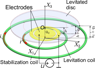
Figure 9: The simplest scheme for preliminary analysis of obtained models: $U$ is the potential applied to electrodes, $h$ is the space between an electrode plane and equilibrium point of proof mass, $h_{l}$ is the levitation height between a plane of coils and equilibrium point of the disc.

For further analysis, model (12) is presented in the dimensionless form as follows

$$\begin{array}[]{l}{\displaystyle\frac{d^{2}\lambda}{d\tau^{2}}+1-\eta\left[\left(\frac{2}{k}-k\right)K(k)-\frac{2}{k}E(k)\right]\frac{2}{k^{2}}}\\ {\displaystyle\times\left[\frac{2-k^{2}}{2(1-k^{2})}E(k)-K(k)\right]\cdot\frac{\kappa\xi^{2}(1+\kappa\lambda)}{(1+\xi^{2}(1+\kappa\lambda)^{2})^{3/2}}}\\ {\displaystyle+\frac{\beta}{(1+\lambda)^{2}}=0,}\end{array}$$ (14)

where $\tau=\sqrt{g/h}t$, $\lambda=q_{3}/h$, $\eta=I^{2}a^{2}/(mghL^{o})$, $\beta=A_{0}U^{2}/(4mgh^{2})$, $\kappa=h/h_{l}$, $a=R_{l}\mu_{0}$ and $\xi=h_{l}/(2R_{l})$.

From Eq. (14), the static pull-in model is

$$\begin{array}[]{l}{\displaystyle\beta=(1+\lambda)^{2}\left(-1+\eta\left[\left(\frac{2}{k}-k\right)K(k)-\frac{2}{k}E(k)\right]\frac{2}{k^{2}}\right.}\\ {\displaystyle\left.\times\left[\frac{2-k^{2}}{2(1-k^{2})}E(k)-K(k)\right]\cdot\frac{\kappa\xi^{2}(1+\kappa\lambda)}{(1+\xi^{2}(1+\kappa\lambda)^{2})^{3/2}}\right),}\\ \end{array}$$ (15)

where the $\eta$ constant can be defined at equilibrium state of the system, when $\lambda$ and $\beta$ are zero, as follows

$$\begin{array}[]{l}{\displaystyle\eta=\left(\left[\left(\frac{2}{k_{0}}-k_{0}\right)K(k_{0})-\frac{2}{k_{0}}E(k_{0})\right]\frac{2}{k_{0}^{2}}\right.}\\ {\displaystyle\left.\times\left[\frac{2-k_{0}^{2}}{2(1-k_{0}^{2})}E(k_{0})-K(k_{0})\right]\cdot\frac{\kappa\xi^{2}}{(1+\xi^{2})^{3/2}}\right)^{-1},}\\ \end{array}$$ (16)

and $k_{0}^{2}=1/(1+\xi^{2})$.

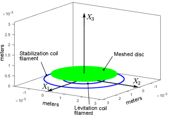
Figure 10: The 3D scheme for simulation: the $3.1\text{\,}\mathrm{mm}$ diameter disc is meshed by 3993 circular elements.

VI Quasi-FEM of static linear pull-in actuation

The quasi-FEM model of the static linear pull-in has a similar form to (12). The difference arises due to the fact that the magnetic interaction between the disc and coils along the $X_{3}$ axis is defined by the force $F_{3}$ from Eq. (10). Hence, taking into account this fact, the quasi-FEM model becomes

$$m\frac{d^{2}q_{3}}{dt^{2}}+mg+\underline{I}^{T}\frac{\partial\underline{M}_{c}}{\partial q_{3}}\underline{I}_{c}+\frac{A_{0}}{4}\frac{U^{2}}{(h+q_{3})^{2}}=0.$$ (17)

Now, we present Eq. (17) in dimensionless from:

$$\begin{array}[]{l}{\displaystyle\frac{d^{2}\lambda}{d\tau^{2}}+1+\eta_{0}F_{m}(\lambda)+\frac{\beta}{(1+\lambda)^{2}}=0};\\ {\displaystyle F_{m}(\lambda)=\sum_{s=1}^{n}\sum_{j=1}^{N}\eta_{sj}\frac{\partial\overline{M}_{sj}(\overline{x}_{1},\overline{x}_{2},(1+\lambda\kappa)\chi)}{\partial\lambda}},\end{array}$$ (18)

where $\eta_{0}=\mu_{0}I_{c1}^{2}\sqrt{R_{c1}R_{e}}/(mgR_{e})$, $R_{c1}$ is the radius of the first winding of the levitation coil, $\eta_{sj}=\overline{I}_{s}\overline{I}_{cj}\sqrt{\overline{R}_{cj}}\Big{/}\chi$, $\overline{I}_{s}=I_{s}/I_{c1}$ and $\overline{I}_{cj}=I_{cj}/I_{c1}$ are the dimensionless currents, $\overline{R}_{cj}=R_{cj}/R_{c1}$, $\chi=h_{l}/R_{e}$ is the scaling factor, $\partial\overline{M}_{sj}/{\partial\lambda}$ is the derivative of dimensionless mutual inductance with respect to $\lambda$ (its definition is shown in Appendix A), $\overline{x}_{1}=x_{1}/R_{e}$ and $\overline{x}_{2}=x_{2}/R_{e}$ are the dimensionless coordinates. Noting that $x_{1}$ and $x_{2}$ are defined by Eq. (11).

The static pull-in model based on quasi-FEM (18) is

$${\displaystyle\beta=-(1+\lambda)^{2}\big{(}1+\eta_{0}F_{m}(\lambda)\big{)}},$$ (19)

where similar to (16) the $\eta_{0}$ constant is also defined at equilibrium state as follows

$${\displaystyle\eta_{0}=-1/F_{m}(0).}$$ (20)

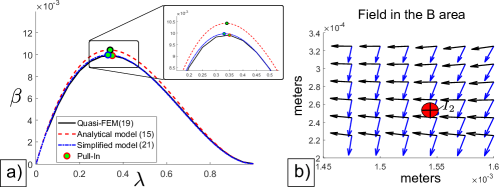
Figure 11: Pull-in actuation of the $3.1\text{\,}\mathrm{mm}$ diameter disc: a) equilibrium curve of the square voltage vs displacement (absolute value of $\lambda$); b) the map of the magnetic field (blue arrows) and its corresponded gradient (black arrows) within the B area build on the $X_{3}$-$X_{2}$ plane around the $I_{2}$ circuit.

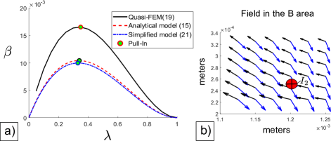
Figure 12: Pull-in actuation of the $2.4\text{\,}\mathrm{mm}$ diameter disc: a) equilibrium curve of the square voltage vs displacement (absolute value of $\lambda$); b) the map of the magnetic field (blue arrows) and its corresponded gradient (black arrows) within the B area build on the $X_{3}$-$X_{2}$ plane around the $I_{2}$ circuit.

VII Preliminary analysis of developed models

It is obvious that if the magnetic field gradient in the B area around the $I_{2}$ circuit of eddy current within the disc and corresponding force is directed almost horizontally (see Fig. 8c)), then the estimation of pull-in parameters by means of the analytical model (15) becomes close to the exact calculation performed by the quasi-FEM (19). This fact indicates that the application of the analytical model requires the knowledge about the gradient of the magnetic field in the B area of a particular design under consideration.

On the other hand, due to design particularities of HLMA there are some particular cases, which can be immediately treated by the model (15) presenting a solution in simple analytical equations. In turn, these simple equations are convenient for the practical application. For instance, let us consider such a particular case, which takes place when dimensionless parameter $\kappa$ is small. From physical point of view, it means that the redistribution between energy stored within the electrical field of capacitors and energy stored within magnetic field of coils and levitated disc occurs by changing the location of electrodes along the $X_{3}$ axis and, in particular, the electrodes are located closer to the levitated disc. This fact leads to the possibility of a linearization of the magnetic force in the analytical model (15). Thus, we can write the following simple model of static pull-in actuation as

$${\displaystyle\beta=-\frac{\ln(4/\xi)-1}{\ln(4/\xi)-2}\kappa\lambda(1+\lambda)^{2}}.$$ (21)

From the later model, the pull-in parameters can be estimated to be

$$\lambda_{p}=-\frac{1}{3},\;\;\;\beta_{p}=\frac{\ln(4/\xi)-1}{\ln(4/\xi)-2}\kappa\frac{4}{27}.$$ (22)

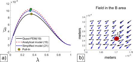
Figure 13: Pull-in actuation of the $3.2\text{\,}\mathrm{mm}$ diameter disc: a) equilibrium curve of the square voltage vs displacement (absolute value of $\lambda$); b) the map of the magnetic field (blue arrows) and its corresponded gradient (black arrows) within the B area build on the $X_{3}$-$X_{2}$ plane around the $I_{2}$ circuit.

TABLE I: Pull-in parameters for the $3.1\text{\,}\mathrm{mm}$ diameter disc.

Model	Pull-in parameter			Relative Error
	$\lambda_{p}$	$\beta_{p}$	$\sqrt{\beta_{p}}$	$\Delta\lambda_{p}$	$\Delta\sqrt{\beta_{p}}$
Quasi-FEM, (19)	0.34	0.0099	0.0995	–	–
Analytical model, (15)	0.34	0.0104	0.102	0	0.025
Simplified model, (21)	0.3333	0.01	0.1	0.0474	0.005

Now let us apply the obtained models, namely, (15), (19) and (21) to the design shown in Fig. 9 and consists of two circular plane coils having radii of $1.0\text{\,}\mathrm{mm}$ and $1.9\text{\,}\mathrm{mm}$ for levitation and stabilization coil, respectively. The disc is levitated at height, $h_{l}$, of $250\text{\,}\mathrm{\SIUnitSymbolMicro m}$, while the electrodes are placed at a point measured from the equilibrium point $O$ of the disc along the $X_{3}$ axis on a distance, $h$, of $10\text{\,}\mathrm{\SIUnitSymbolMicro m}$. Hence, the dimensionless parameters of the design become $\kappa=0.04$ and $\xi=0.125$. Then, according to Eq. (22) the square dimensionless pull-in voltage can be calculated and becomes $\beta_{p}=1.4930\frac{4}{27}=0.01$. The modelling is performed for a disc with the following radii: $1.2\text{\,}$, $1.55\text{\,}$ and $1.7\text{\,}\mathrm{mm}$. Fig. 10 depicts the 3D scheme for simulation. The disc is meshed by 3993 circular elements.

The three equilibrium curves of pull-in actuation for a disc having a diameter of $1.55\text{\,}\mathrm{mm}$ calculated by models (15), (19) and (21) are shown in Fig. 11a). Results of estimation of pull-in parameters are summed up in Table I. The simulation shows that the pull-in displacement (in absolute value) is $\lambda_{p}=0.34$ and the pull-in voltage is $\sqrt{\beta_{p}}=0.0995$. The relative errors of estimation of pull-in parameters by means of the analytical models do not exceed $5\text{\,}\%$ (please see Table I). Noting that the map of gradient of the magnetic field in the B area is directed almost horizontally as shown in Fig.11b). Hence, the contribution of electromagnetic force due to interaction between the magnetic field and the $I_{2}$ circuit to the pull-in actuation is small.

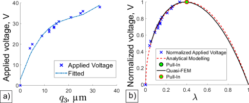
Figure 14: Pull-in actuation of disc having a $2.4\text{\,}\mathrm{mm}$ diameter: a) experimental measurement of applied voltage vs linear displacement; b) normalized voltage vs dimensionless displacement: measurement data together with equilibrium curves generated by quasi-FEM and analytical one.

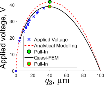
Figure 15: Two equilibrium curves calculated by quasi-FEM Eq. (17) and analytical model Eq. (12) of applied voltage vs displacement of the disc having a $2.4\text{\,}\mathrm{mm}$ diameter in comparing with experimental data.

Fig. 12a) shows the equilibrium curve of pull-in actuation for a disc having a diameter of $2.4\text{\,}\mathrm{mm}$, which is simulated by quasi-FEM (19). Since the analytical models (15) and (21) are independent of a radius of the levitated disc, the results of modelling are the same as presented in Fig.11a) and Table I. The simulation predicts the following values of the pull-in parameters such as

$$\lambda_{p}=0.34,\;\;\;\beta_{p}=0.01653,\;\;\;\sqrt{\beta_{p}}=0.1286,$$ (23)

where the dimensionless displacement $\lambda_{p}$ is given in absolute value. Although, the pull-in displacement has the same value as in the previous example, the main difference appears in the estimation of the pull-in voltage, which is increased due to the contribution of the electromagnetic force exerted on the $I_{2}$ circuit as shown in Fig. 12b). As a result, the relative error of the calculation of pull-in voltage by means of the analytical models is also increased drastically to $30\text{\,}\%$.

In the case of the $3.4\text{\,}\mathrm{mm}$ diameter disc, the equilibrium curve simulated by quasi-FEM (19) is shown in Fig. 13a). The simulation predicts the following pull-in parameters such as

$$\lambda_{p}=0.34,\;\;\;\beta_{p}=0.009,\;\;\;\sqrt{\beta_{p}}=0.0949.$$ (24)

In this case, the calculation of pull-in voltage by means of analytical models shows that the relative error is around $5\text{\,}\%$. As seen, the value of the pull-in voltage is decreased due to the electromagnetic force acting on the $I_{2}$ circuit, which has a vertical component directed against the levitation force as shown in Fig. 13b).

Noting that in all three cases considered above, the map of the magnetic field and the corresponded gradient in the A area is similar to the map shown in Fig. 8b).

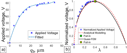
Figure 16: Pull-in actuation of disc having a $2.8\text{\,}\mathrm{mm}$ diameter: a) experimental measurement of applied voltage vs linear displacement [19]; b) normalized voltage vs dimensionless displacement: measurement data together with equilibrium curves generated by quasi-FEM and analytical one.

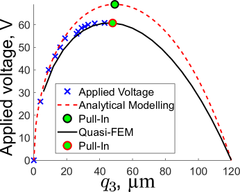
Figure 17: Two equilibrium curves calculated by quasi-FEM Eq. (17) and analytical model Eq. (12) of applied voltage vs displacement of the disc having a $2.8\text{\,}\mathrm{mm}$ diameter in comparing with experimental data.

VIII Comparison with experiment

Now let us compare the results of simulation and modelling generated by the quasi-FEM and analytical model, respectively, with experimental data reported in [19, 39] for linear pull-in actuation performed by two discs having diameters of $2.8\text{\,}$ and $3.2\text{\,}\mathrm{mm}$ in the prototype of HLMA presented in Sec. III. Also, we added new experimental data collected in the same prototype for the $3.2\text{\,}\mathrm{mm}$ diameter disc and a lighter disc of a $2.4\text{\,}\mathrm{mm}$ diameter.

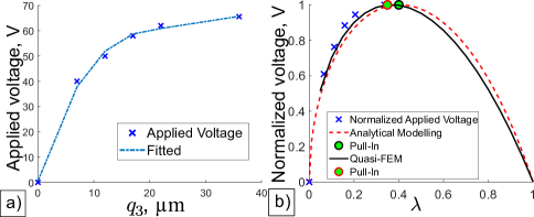
Figure 18: Pull-in actuation of disc having a $3.2\text{\,}\mathrm{mm}$ diameter and levitated at $107\text{\,}\mathrm{\SIUnitSymbolMicro m}$: a) experimental measurement of applied voltage vs linear displacement [39]; b) normalized voltage vs dimensionless displacement: measurement data together with equilibrium curves generated by quasi-FEM and analytical one.

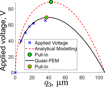
Figure 19: Two equilibrium curves calculated by quasi-FEM Eq. (17) and analytical model Eq. (12) of applied voltage vs displacement of the disc having a $3.2\text{\,}\mathrm{mm}$ diameter and levitated at $107\text{\,}\mathrm{\SIUnitSymbolMicro m}$ in comparing with experimental data.

VIII-A A light disc of a $2.4\text{\,}\mathrm{mm}$ diameter

Fig. 14a) shows the result of the measurement of applied voltage to the electrodes 1 and 2 (see, Fig.3b)) against the displacement of the disc having a $2.4\text{\,}\mathrm{mm}$ diameter. The disc was levitated at a height of $100\text{\,}\mathrm{\SIUnitSymbolMicro m}$ metering from the electrode plane and its displacement was measured by the laser sensor. The pull-in actuation occurred at a height of $75\text{\,}\mathrm{\SIUnitSymbolMicro m}$ corresponding to the pull-in displacement of $35\text{\,}\mathrm{\SIUnitSymbolMicro m}$ upon applying $38\text{\,}\mathrm{V}$ to the electrodes. Fig. 14b) shows the comparison of equilibrium curves generated by quasi-FEM (19) and analytical model (15) with experimental measurement in normalized voltage. For the simulation, the 3D geometrical scheme as shown in Fig. 6 with same dimensions for coils are used. The disc is meshed by 3993 elements as shown in Fig. 4. The modelling is carried out with the following dimensionless parameters: $\xi=0.09$ and $\kappa=0.55$. Analysis of Fig. 14b) depicts a good agreement between both developed models itself. In particular, both models predict the same value of the pull-in displacement. Only, we see a slight difference between the shapes of the curves after the pull-in point. Also, both models in terms of normalized values are in good agreement with experiment. However, the comparison in terms of dimension values shown in Fig. 15 reveals that the analytical model gives a relative error, which is around $16\text{\,}\%$ in estimation of the pull-in voltage.

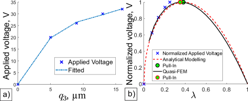
Figure 20: Pull-in actuation of disc having a $3.2\text{\,}\mathrm{mm}$ diameter and levitated at $64\text{\,}\mathrm{\SIUnitSymbolMicro m}$: a) experimental measurement of applied voltage vs linear displacement; b) normalized voltage vs dimensionless displacement: measurement data together with equilibrium curves generated by quasi-FEM and analytical one.

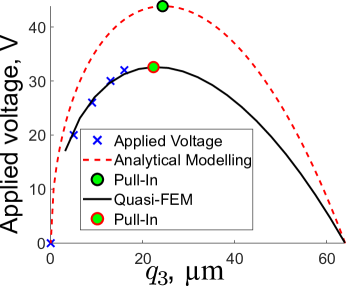
Figure 21: Two equilibrium curves calculated by quasi-FEM Eq. (17) and analytical model Eq. (12) of applied voltage vs displacement of the disc having a $3.2\text{\,}\mathrm{mm}$ diameter and levitated at $64\text{\,}\mathrm{\SIUnitSymbolMicro m}$ in comparing with experimental data.

TABLE II: Results of measurements and modelling of the static pull-in actuation.

Measured parameters	Diameter of disc	$2.4\text{\,}\mathrm{mm}$	$2.8\text{\,}\mathrm{mm}$	$3.2\text{\,}\mathrm{mm}$
	Mass of disc	$0.2\text{\,}\mathrm{mg}$	$0.3\text{\,}\mathrm{mg}$	$0.7\text{\,}\mathrm{mg}$
	Levitation height, $h_{l}$	$180\text{\,}\mathrm{\SIUnitSymbolMicro m}$	$200\text{\,}\mathrm{\SIUnitSymbolMicro m}$	$144\text{\,}\mathrm{\SIUnitSymbolMicro m}$	$187\text{\,}\mathrm{\SIUnitSymbolMicro m}$
	Spacing, $h$	$100\text{\,}\mathrm{\SIUnitSymbolMicro m}$	$119\text{\,}\mathrm{\SIUnitSymbolMicro m}$	$64\text{\,}\mathrm{\SIUnitSymbolMicro m}$	$107\text{\,}\mathrm{\SIUnitSymbolMicro m}$
Calculated parameters	$\xi=h_{l}/(2R_{l})$	0.09	0.1	0.072	0.0935
	$\kappa=h/h_{l}$	0.55	0.6	0.44	0.57
Measured pull-in	Displacement	$35\text{\,}\mathrm{\SIUnitSymbolMicro m}$	$43\text{\,}\mathrm{\SIUnitSymbolMicro m}$	$18\text{\,}\mathrm{\SIUnitSymbolMicro m}$	$36\text{\,}\mathrm{\SIUnitSymbolMicro m}$
parameters	Voltage	$38\text{\,}\mathrm{V}$	$60.8\text{\,}\mathrm{V}$	$32\text{\,}\mathrm{V}$	$65\text{\,}\mathrm{V}$
Pull-in parameters	Displacement	$40\text{\,}\mathrm{\SIUnitSymbolMicro m}$	$49\text{\,}\mathrm{\SIUnitSymbolMicro m}$	$24\text{\,}\mathrm{\SIUnitSymbolMicro m}$	$42\text{\,}\mathrm{\SIUnitSymbolMicro m}$
modelled by Eq.(12)	Voltage	$43\text{\,}\mathrm{V}$	$69\text{\,}\mathrm{V}$	$44\text{\,}\mathrm{V}$	$88\text{\,}\mathrm{V}$
Pull-in parameters	Displacement	$40\text{\,}\mathrm{\SIUnitSymbolMicro m}$	$48\text{\,}\mathrm{\SIUnitSymbolMicro m}$	$22\text{\,}\mathrm{\SIUnitSymbolMicro m}$	$37\text{\,}\mathrm{\SIUnitSymbolMicro m}$
simulated by Eq.(17)	Voltage	$37\text{\,}\mathrm{V}$	$60.76\text{\,}\mathrm{V}$	$33\text{\,}\mathrm{V}$	$69\text{\,}\mathrm{V}$

VIII-B Disc of a $2.8\text{\,}\mathrm{mm}$ diameter

Fig. 16a) presents the result of the measurement of pull-in actuation of the disc having a $2.8\text{\,}\mathrm{mm}$ diameter, which was obtained in our work [19]. The disc was levitated at a height of $120\text{\,}\mathrm{\SIUnitSymbolMicro m}$ measuring from the electrode plane. The pull-in actuation occurred at a height of $77\text{\,}\mathrm{\SIUnitSymbolMicro m}$ corresponding to the pull-in displacement of $43\text{\,}\mathrm{\SIUnitSymbolMicro m}$ upon applying $60.8\text{\,}\mathrm{V}$ to the electrodes. The simulation is performed in a similar way as it was discussed in the previous section VIII-A. The difference is only in a size of diameter of the disc and a levitation height. For modeling, the following dimensionless parameters, namely, $\xi=0.1$ and $\kappa=0.6$ are used. Comparison of both models in normalized values as shown in Fig. 16b) depicts a difference between the pull-in displacements predicted by quasi-FEM (19) and analytical model (15). The analytical model (15) gives a relative error, which is around $2\text{\,}\%$ in estimation of the pull-in displacement. Also, there is a slight difference between the shapes of the curves after the pull-in point, similar to the previous result. Conducting the analysis in terms of dimension values as shown in Fig. 17, the relative error of around $13\text{\,}\%$ produced by the analytical model in the calculation of the pull-in voltage can be recognized.

VIII-C Disc of a $3.2\text{\,}\mathrm{mm}$ diameter

The result of the experimental investigation of the pull-in actuation in the presented prototype of HLMA with the disc of a $3.2\text{\,}\mathrm{mm}$ diameter was discussed and reported in our work [39]. Measuring from the electrode plane, the disc was levitated at a height of $107\text{\,}\mathrm{\SIUnitSymbolMicro m}$. Fig. 18a) shows the measurement of applied voltage to the electrodes against the disc linear displacement along the vertical axis. The pull-in actuation occurred at a height of $71\text{\,}\mathrm{\SIUnitSymbolMicro m}$ corresponding to the pull-in displacement of $36\text{\,}\mathrm{\SIUnitSymbolMicro m}$ upon applying $65\text{\,}\mathrm{V}$ to the electrodes. The results of simulation and modelling are shown in Fig. 18b) in the normalized values. The analysis of Fig. 18b) reveals a slight shift on the right of the equilibrium curve generated by the analytical model (15) with respect to the curve modeled by the quasi-FEM (19).

Hence, this shift corresponds to the $13.5\text{\,}\%$ relative error in calculation of the pull-in displacement by the analytical model. The relative error produced by the analytical model in estimation of the pull-in voltage is calculated to be $30\text{\,}\%$ as follows from the analysis of the results of simulation and modelling in dimension values shown in Fig. 19.

In addition we add new data of measurement of the pull-in actuation performed by the same disc, which was levitated at a height of $64\text{\,}\mathrm{\SIUnitSymbolMicro m}$. The result of measurement of applied voltage against the linear displacement of the disc is shown in Fig. 20. The pull-in actuation occurred at a height of $46\text{\,}\mathrm{\SIUnitSymbolMicro m}$ corresponding the pull-in displacement of $18\text{\,}\mathrm{\SIUnitSymbolMicro m}$ upon applying the pull-in voltage equal to $32\text{\,}\mathrm{V}$. Similar to Fig. 18b), the equilibrium curve generated by the analytical model has a slight shift on the right relative to the curve generated by the quasi-FEM as shown in Fig. 20b). This shift corresponds to the $9\text{\,}\%$ relative error given by the analytical model in the estimation of the pull-in displacement. Comparing in terms of dimension values as shown in Fig. 21, the relative error of around $28\text{\,}\%$ produced by the analytical model in the calculation of the pull-in voltage is appeared.

The all results of measurements and modelling of the pull-parameters including related particularities of the experiments and values of dimensionless parameters for modelling are summed up in Table. II.

IX Discussion and conclusion

In this work, the quasi-finite element method to model the static and dynamic behavior of electromagnetic levitation micro-actuators based on the Lagrangian formalism has been developed. The particularity of obtained quasi-finite element method is the combination of finite element manner to calculate induced eddy current within a levitated micro-object and the set of six differential equations describing the behavior of mechanical part of electromagnetic levitation system. Using a circular filament as a finite element for meshing the levitated micro-object, on the one hand, allows to covering any shapes of the micro-object levitated by a system of wire-loops. On the other hand, it allows to reducing the calculation of the mutual inductance between the system of arbitrary shape wire loops and the levitated micro-object to a line integral as it was shown by Kalantarov and Zeitlin. As a result, static and dynamic characteristics of an electromagnetic levitation system including the analysis of its stability can be calculated and studied.

In particular, the developed method was applied to study static pull-actuation performed by the hybrid levitation micro-actuator. In general, the pull-in parameters of HLMA are a nonlinear function of its design due to the magnetic field generated by coil currents. However, the developed model allows us to calculate accurately the pull-in parameters of HLMA for different diameters of disc levitated at different heights. The pull-in parameters are gathered under the following condition. Namely, disc is meshed by 3993 elements and coils are represented by 32 circular filaments. The time of calculation of one point was about $120\text{\,}\mathrm{s}$. For building equilibrium curve, fifteen points were used. The comparison of simulation results generated by the model (19) based on quasi-finite element method with the experiment shows a good agreement between the theory and measurement. This fact confirms the efficiency of the developed method.

At the same time, the analytical model (15) based on the approximation of induced eddy current within the disc by one eddy current circuits was proposed as a result of the analysis of the distribution of the eddy current and the magnetic field generated by coil currents. Although, the effective use of the analytical model requires the knowledge about the gradient of the magnetic field of a particular design under consideration. However, arising some particular cases, for instance, when electrodes, to generate electrostatic force acting on the disc, located very close to the disc bottom surface (dimensionless parameter, $\kappa$, is small, less than 0.1), the simple analytical equation (21) for estimation of the pull-in parameters with errors not exceeding $5\text{\,}\%$ can be obtained.

Appendix A The derivative of dimensionless mutual inductance with respect to $\lambda$

Due to the particularity of the problem, namely, there is no angular misalignment between a circular element and a coil. Hence, the original formula for calculation of the mutual inductance between two circular filaments based on the Kalantarov-Zeitlin approach [31] in a dimensionless form can be rewritten as follows:

$$\overline{M}_{sj}=\frac{1}{\pi}\int_{0}^{2\pi}\frac{1+\overline{x}_{1}\cdot\cos\varphi+\overline{x}_{2}\cdot\sin\varphi}{\bar{\rho}^{1.5}}\frac{\Psi(k)}{k}d\varphi,$$ (25)

where

$$\bar{\rho}=\sqrt{1+2(\overline{x}_{1}\cdot\cos\varphi+\overline{x}_{2}\cdot\sin\varphi)+\overline{x}_{1}^{2}+\overline{x}_{2}^{2}};$$ (26)

$$\Psi(k)=\left(1-\frac{k^{2}}{2}\right)K(k)-E(k),$$ (27)

where $K(k)$ and $E(k)$ are the complete elliptic functions of the first and second kind, respectively;

$$k^{2}=\frac{4\nu_{j}\bar{\rho}}{(\nu_{j}\bar{\rho}+1)^{2}+\nu_{j}^{2}\overline{x}_{3}^{2}},$$ (28)

where $\nu_{j}=R_{e}/R_{cj}$, $R_{cj}$ is the radius of the $j$-coil filament, $\overline{x}_{1}$, $\overline{x}_{2}$ and $\overline{x}_{3}$ are the components of the radius vector $\boldsymbol{{r}}$ in base ${\boldsymbol{\underline{e}}^{z}}$ (see Eq. (11)).

The derivative of dimensionless mutual inductance with respect to $\overline{x}_{3}$ is

$$\frac{\partial\overline{M}_{sj}}{\partial\overline{x}_{3}}=\frac{1}{\pi}\int_{0}^{2\pi}\frac{1+\overline{x}_{1}\cdot\cos\varphi+\overline{x}_{2}\cdot\sin\varphi}{\bar{\rho}^{1.5}}\Phi(k)d\varphi,$$ (29)

where

$$\Phi(k)=\frac{d}{d\overline{x}_{3}}\frac{\Psi(k)}{k}=\frac{1}{k^{2}}\left(\frac{2-k^{2}}{2(1-k^{2})}E(k)-K(k)\right)\frac{dk}{d\overline{x}_{3}},$$ (30)

$$\frac{dk}{d\overline{x}_{3}}=-\frac{\nu_{j}^{2}\overline{x}_{3}\sqrt{4\nu_{j}\bar{\rho}}}{\left((1+\nu_{j}\bar{\rho})^{2}+\nu_{j}^{2}\overline{x}_{3}^{2}\right)^{3/2}}.$$ (31)

Substituting $\overline{x}_{3}=\lambda\kappa\chi$ into Eq. (29), the desired equation for the derivative of dimensionless mutual inductance with respect to $\lambda$ is derived.

References

- [1] K. V. Poletkin, A. Asadollahbaik, R. Kampmann, and J. G. Korvink, “Levitating micro-actuators: A review,” Actuators, vol. 7, no. 2, 2018. [Online]. Available: http://www.mdpi.com/2076-0825/7/2/17
- [2] J. Jin, T. C. Yih, T. Higuchi, and J. U. Jeon, “Direct electrostatic levitation and propulsion of silicon wafer,” IEEE Transactions on Industry Applications, vol. 34, no. 5, pp. 975–984, 1998.
- [3] T. Murakoshi, Y. Endo, K. Fukatsu, S. Nakamura, and M. Esashi, “Electrostatically levitated ring-shaped rotational gyro/accelerometer,” Jpn. J. Appl. Phys, vol. 42, no. 4B, pp. 2468–2472, 2003.
- [4] F. Han, Y. Liu, L. Wang, and G. Ma, “Micromachined electrostatically suspended gyroscope with a spinning ring-shaped rotor,” Journal of Micromechanics and Microengineering, vol. 22, no. 10, p. 105032, 2012.
- [5] F. Han, B. Sun, L. Li, and Q. Wu, “Performance of a sensitive micromachined accelerometer with an electrostatically suspended proof mass,” IEEE Sensors J., vol. 15, pp. 209 – 217, 2015.
- [6] T. Coombs, I. Samad, D. Ruiz-Alonso, and K. Tadinada, “Superconducting micro-bearings,” Applied Superconductivity, IEEE Transactions on, vol. 15, no. 2, pp. 2312–2315, 2005.
- [7] Z. Lu, K. Poletkin, B. den Hartogh, U. Wallrabe, and V. Badilita, “3D micro-machined inductive contactless suspension: Testing and modeling,” Sensors and Actuators A Physical, vol. 220, pp. 134–143, 2014. [Online]. Available: http://dx.doi.org/10.1016/j.sna.2014.09.017
- [8] K. Poletkin, A. Moazenzadeh, S. G. Mariappan, Z. Lu, U. Wallrabe, J. G. Korvink, and V. Badilita, “Polymer magnetic composite core boosts performance of 3D micromachined inductive contactless suspension,” IEEE Magnetics Letters, vol. 7, pp. 1–3, 2016. [Online]. Available: http://dx.doi.org/10.1109/LMAG.2016.2612181
- [9] C. Shearwood, C. B. Williams, P. H. Mellor, K. Y. Chang, and J. Woodhead, “Electro-magnetically levitated micro-discs,” in IEE Colloquium on Microengineering Applications in Optoelectronics, Feb 1996, pp. 6/1–6/3.
- [10] Q. Xiao, M. Kraft, Z. Luo, J. Chen, and J. Wang, “Design of contactless electromagnetic levitation and electrostatic driven rotation control system for a micro mirror,” in 2018 15th International Conference on Control, Automation, Robotics and Vision (ICARCV), Nov 2018, pp. 1176–1179.
- [11] C. Shearwood, K. Ho, C. Williams, and H. Gong, “Development of a levitated micromotor for application as a gyroscope,” Sensor. Actuat. A-Phys., vol. 83, no. 1-3, pp. 85–92, 2000.
- [12] Y. Su, Z. Xiao, Z. Ye, and K. Takahata, “Micromachined graphite rotor based on diamagnetic levitation,” IEEE Electron Device Lett., vol. 36, no. 4, pp. 393–395, 2015.
- [13] D. Garmire, H. Choo, R. Kant, S. Govindjee, C. Sequin, R. Muller, and J. Demmel, “Diamagnetically levitated MEMS accelerometers,” in Solid-State Sensors, Actuators and Microsystems Conference, 2007. TRANSDUCERS 2007. International. IEEE, 2007, pp. 1203–1206.
- [14] C. Dieppedale, B. Desloges, H. Rostaing, J. Delamare, O. Cugat, and J. Meunier-Carus, “Magnetic bistable micro-actuator with integrated permanent magnets,” in Proc. IEEE Sensors, vol. 1, Oct. 2004, pp. 493–496.
- [15] J. Abadie, E. Piat, S. Oster, and M. Boukallel, “Modeling and experimentation of a passive low frequency nanoforce sensor based on diamagnetic levitation,” Sensor. Actuat. A-Phys., vol. 173, no. 1, pp. 227–237, 2012.
- [16] W. Liu, W.-Y. Chen, W.-P. Zhang, X.-G. Huang, and Z.-R. Zhang, “Variable-capacitance micromotor with levitated diamagnetic rotor,” Electronics Letters, vol. 44, no. 11, pp. 681–683, 2008.
- [17] Y. Xu, Q. Cui, R. Kan, H. Bleuler, and J. Zhou, “Realization of a diamagnetically levitating rotor driven by electrostatic field,” IEEE/ASME Transactions on Mechatronics, vol. 22, no. 5, pp. 2387–2391, Oct 2017.
- [18] I. Sari and M. Kraft, “A MEMS linear accelerator for levitated micro-objects,” Sensor. Actuat. A-Phys., vol. 222, pp. 15–23, 2015.
- [19] K. Poletkin, Z. Lu, U. Wallrabe, and V. Badilita, “A new hybrid micromachined contactless suspension with linear and angular positioning and adjustable dynamics,” Journal of Microelectromechanical Systems, vol. 24, no. 5, pp. 1248–1250, Oct. 2015.
- [20] K. V. Poletkin, “A novel hybrid contactless suspension with adjustable spring constant,” in 2017 19th International Conference on Solid-State Sensors, Actuators and Microsystems (TRANSDUCERS), June 2017, pp. 934–937.
- [21] K. V. Poletkin and J. G. Korvink, “Modeling a pull-in instability in micro-machined hybrid contactless suspension,” Actuators, vol. 7, no. 1, 2018. [Online]. Available: http://www.mdpi.com/2076-0825/7/1/11
- [22] K. V. Poletkin, A. I. Chernomorsky, and C. Shearwood, “A proposal for micromachined accelerometer, base on a contactless suspension with zero spring constant,” IEEE Sensors J., vol. 12, no. 07, pp. 2407–2413, 2012.
- [23] D. Elata and H. Bamberger, “On the dynamic pull-in of electrostatic actuators with multiple degrees of freedom and multiple voltage sources,” Journal of Microelectromechanical systems, vol. 15, no. 1, pp. 131–140, 2006.
- [24] I. Ciric, “Electromagnetic levitation in axially symmetric systems,” Rev. Roum. Sci. Tech. Ser. Electrotech. & Energ, vol. 15, no. 1, pp. 35–73, 1970.
- [25] C. Williams, C. Shearwood, P. Mellor, and R. Yates, “Modelling and testing of a frictionless levitated micromotor,” Sensors and Actuators A: Physical, vol. 61, no. 1, pp. 469–473, 1997.
- [26] W. Zhang, W. Chen, X. Zhao, X. Wu, W. Liu, X. Huang, and S. Shao, “The study of an electromagnetic levitating micromotor for application in a rotating gyroscope,” Sensor. Actuat. A-Phys., vol. 132, no. 2, pp. 651–657, 2006.
- [27] K. Liu, W. Zhang, W. Liu, W. Chen, K. Li, F. Cui, and S. Li, “An innovative micro-diamagnetic levitation system with coils applied in micro-gyroscope,” Microsystem Technologies, vol. 16, no. 3, p. 431, Nov 2009. [Online]. Available: https://doi.org/10.1007/s00542-009-0935-x
- [28] Z. Lu, F. Jia, J. G. Korvink, U. Wallrabe, and V. Badilita, “Design optimization of an electromagnetic microlevitation system based on copper wirebonded coils,” in Proceedings of PowerMEMS 2012, Atlanta, GA, USA, 2012, pp. 363–366.
- [29] E. Laithwaite, “Electromagnetic levitation,” Electrical Engineers, Proceedings of the Institution of, vol. 112, no. 12, pp. 2361–2375, 1965.
- [30] S. Babic, F. Sirois, C. Akyel, and C. Girardi, “Mutual inductance calculation between circular filaments arbitrarily positioned in space: alternative to Grover’s formula,” IEEE Transactions On Magnetics, vol. 46, pp. 3591–3600, 2010.
- [31] K. V. Poletkin and J. G. Korvink, “Efficient calculation of the mutual inductance of arbitrarily oriented circular filaments via a generalisation of the kalantarov-zeitlin method,” Journal of Magnetism and Magnetic Materials, vol. 483, pp. 10–20, 2019. [Online]. Available: http://www.sciencedirect.com/science/article/pii/S0304885318337703
- [32] K. Poletkin, A. Chernomorsky, C. Shearwood, and U. Wallrabe, “A qualitative analysis of designs of micromachined electromagnetic inductive contactless suspension,” International Journal of Mechanical Sciences, vol. 82, pp. 110–121, May 2014. [Online]. Available: http://authors.elsevier.com/sd/article/S0020740314000897
- [33] K. V. Poletkin, Z. Lu, U. Wallrabe, J. G. Korvink, and V. Badilita, “A qualitative technique to study stability and dynamics of micro-machined inductive contactless suspensions,” in 2017 19th International Conference on Solid-State Sensors, Actuators and Microsystems (TRANSDUCERS), June 2017, pp. 528–531.
- [34] K. Poletkin, Z. Lu, U. Wallrabe, J. Korvink, and V. Badilita, “Stable dynamics of micro-machined inductive contactless suspensions,” International Journal of Mechanical Sciences, vol. 131-132, pp. 753–766, 2017. [Online]. Available: http://www.sciencedirect.com/science/article/pii/S0020740316306555
- [35] J. Wittenburg, Dynamics of multibody systems. Springer Science & Business Media, 2007.
- [36] Y. G. Martynenko, Analytical dynamics of electromechanical systems. Izd. Mosk. Ehnerg. Inst., Moscow, 1985.
- [37] B. G. Levich, Theoretical physics. An advanced text. vol. 2: Statistical physics. Electromagnetic processes in matter. Amsterdam; London: North-Holland Publishing, 1971.
- [38] K. Poletkin, A. I. Chernomorsky, C. Shearwood, and U. Wallrabe, “An analytical model of micromachined electromagnetic inductive contactless suspension.” in the ASME 2013 International Mechanical Engineering Congress & Exposition. San Diego, California, USA: ASME, Nov. 2013, pp. V010T11A072–V010T11A072. [Online]. Available: http://dx.doi.org/10.1115/IMECE2013-66010
- [39] K. Poletkin, Z. Lu, U. Wallrabe, and V. Badilita, “Hybrid electromagnetic and electrostatic micromachined suspension with adjustable dynamics,” J. Phys.: Conf. Series, vol. 660, no. 1, p. 012005, 2015.
- [40] K. V. Poletkin, R. Shalati, J. G. Korvink, and V. Badilita, “Pull-in actuation in hybrid micro-machined contactless suspension,” Journal of Physics: Conference Series, vol. 1052, p. 012035, jul 2018. [Online]. Available: https://doi.org/10.1088%2F1742-6596%2F1052%2F1%2F012035
- [41] E. Rosa and F. Grover, Formulas and tables for the calculation of mutual and self-inductance. Chicago: US Dept. of Commerce and Labor, Bureau of Standards, 1912.
- [42] H. B. Dwight, Tables of integrals and other mathematical data, 4th ed. New York: The MacMillan Company, 1961.