*

Abstract

Point process models have been used to analyze interaction event times on a social network, in the hope to provides valuable insights for social science research. However, the diagnostics and visualization of the modeling results from such an analysis have received limited discussion in the literature. In this paper, we develop a systematic set of diagnostic tools and visualizations for point process models fitted to data from a network setting. We analyze the residual process and Pearson residual on the network by inspecting their structure and clustering structure. Equipped with these tools, we can validate whether a model adequately captures the temporal and/or network structures in the observed data. The utility of our approach is demonstrated using simulation studies and point process models applied to a study of animal social interactions.

1 Introduction

Interaction event times observed on a social network provide valuable information for social scientists to gain insight into the dynamics and dependence structure among actors on this network. Williamson et al. (2016) studies the social interaction patterns of group-housed male mice over long time periods. In Figure 1-(a), we plot the univariate event times from one pair of mice, which show irregular event-intense intervals and heterogeneity in event densities. Figure 1-(b) displays the observed social interactions among one cohort of mice over time. The interaction patterns appear to be heterogeneous and structured across the social network. We will apply the proposed diagnostic tools to analyses of this data set as real data examples throughout this paper.

A number of continuous-time social network event times models have been recently developed. Saito et al. (2009) studies the cross-reference network of blogs and proposes a model for topic propagation diffusion dynamics. Fan and Shelton (2009) considers a continuous-time Bayesian network with time-varying nodal attributes. Point process models with network dependence structure have become common practice for such studies, with a focus on intensity function estimation (e.g., Perry and Wolfe, 2013; Linderman and Adams, 2014; Zipkin et al., 2016; Yang et al., 2017). In Section 2, we provide a short review of point process models and existing strategies for incorporating network structure.

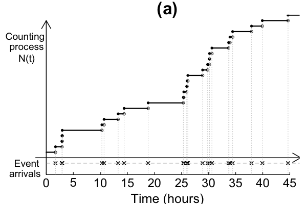
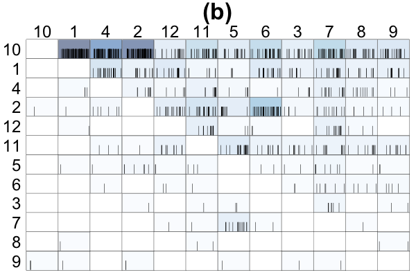
Figure 1: Interaction event times on a social network of mice from Williamson et al. (2016). (a) The univariate point process between one pair of mice. The crosses on the bottom indicating the observed event times. The counting process $N(t)$, defined as the number of events observed up to time $t$, is plotted. (b) Network point processes. Each row represents the initiator (sender) and each column indicates the recipient (receiver) for a social interaction. The rows (columns) are reordered by the I&SI rank (Schmid and de Vries, 2013), where the top row (left column) is the most dominant mouse. The I&SI ranking is a widely used dominance ranking method from animal behavior literature. For the square at $i$-th row and $j$-th column, the observed event times from $i$ to $j$ are plotted as line segments at the bottom. The color shade reflects the total number of events for each pair, with darker color representing more events.

Despite the amount of effort that has been devoted to developing such models, there is limited work on the assessment and diagnostics of those models. To summarize and compare a model’s performance, the likelihood of the model with respect to the observed data is usually evaluated. As an overall assessment of model fit, however, it does not provide detail for detecting when, where, and how the proposed model inadequately accounts for patterns and variations in the observed data. Especially, for interaction dynamics on a social network, the timing often exhibits a bursty and heavy-tailed pattern (Barabasi, 2005), while the structure of interdependence among network actors can be heterogeneous and complicated. Further model developments for addressing these challenges call for the development of better tools that allow researchers to systematically examine and identify the lack-of-fit of existing models against observed data.

The goal of this paper is to propose diagnostic statistics and visualization tools for network event times models, which we develop as extensions of evaluation techniques for univariate point process models. We investigate the proposed techniques using simulated studies and real data. In Section 2, we introduce the notation for point processes, network point processes, and related models. Section 3 focuses on time-domain diagnoses by applying the time rescaling theorem and inspecting residual processes. The diagnostic tools for detecting network heterogeneity and network structure in residual processes are developed and demonstrated in Section 4.

2 Background

2.1 Univariate point processes

Let $(0,T]$ be the time interval of observation. We denote the history of arrival times of observed events up to $T$ as $\mathcal{H}(T)=\{t_{m}\}_{m=0}^{M}$, where $t_{0}=0$, $t_{M}=T$, and $M$ is the total number of events. Figure 1-(a) is a point process of interaction event times between one pair of mice from the animal behavior study in Williamson et al. (2016). The associated univariate point process is defined via a counting process, $N(t)$, $t\in(0,T]$, where $N(t)$ is a right-continuous function that records the number of events observed during the interval $(0,t]$. The stochastic properties of a point process is usually specified by its conditional intensity function $\lambda(t|\mathcal{H}(t))$ at any time $t$,

$$\lambda(t|\mathcal{H}(t))=\lim_{\Delta t\to 0}\frac{Pr([N(t+\Delta t)-N(t)]=1|\mathcal{H}(t))}{\Delta t}.$$

Inference on the intensity function is conducted by evaluating the likelihood function,

$$\prod_{m=1}^{M}\lambda(t_{m}|\mathcal{H}(t_{m}))\exp\Big{\{}-\int_{0}^{T}\lambda(s|\mathcal{H}(s))ds\Big{\}}.$$

A homogeneous Poisson process is the simplest model and assumes a constant intensity $\lambda(t)\equiv\lambda,\lambda>0$. It cannot accommodate situations where event densities vary as shown in Figure 1-(a). A Hawkes process (Hawkes, 1971) is a self-exciting process whose intensity has the form

$$\lambda(t)=\lambda_{1}+\sum_{t_{m}<t}\phi_{\theta}(t-t_{m}),$$

where $\phi_{\theta}(t)$ is a self-exciting kernel with parameter $\theta$. The exponential kernel $\phi(t)=\alpha\exp{(-\beta t)}$ is most widely-used, where $\alpha>0$ calibrates the instantaneous boost to the event intensity at each arrival of an event, and $\beta>0$ controls the decay of past events’ influence over time.

When event dynamics display a bimodal pattern, for example, an alternation between long waiting times and intervals of more intensive events, some models assume that the intensity is modulated by a latent continuous-time Markov chain, $Z(t)$. Here, a $Z(t)$ with $S$-states is parameterized by its infinitesimal generator matrix $Q\in\mathbb{R}^{S\times S}$ (Rabiner, 1989). To accommodate these bimodal patterns, Fischer and Meier-Hellstern (1993) proposed a Markov-modulated Poisson Process (MMPP) model whose intensity function is $\lambda_{Z(t)}$. When the Markov process $Z(t)$ is in state $s\ (s=1,...,S)$, arrivals occur according to a homogeneous Poisson process of rate $\lambda_{s}$. Instead of simply using a constant rate $\lambda_{s}$ in the MMPP, Wang et al. (2012) assumes Hawkes processes with piecewise constant kernel functions as Markov-modulated Hawkes processes with stepwise decay (MMHPSD). The inference procedure heavily relies on the piecewise constant assumption. As a result, MMHPSD suffers from the problem that the inferred latent state is highly sensitive to single events and hard to interpret. Wu et al. (2019) introduces the more widely-used exponential kernel for $\lambda_{s}(t)$ in the Markov-modulated Hawkes Process (MMHP) model under the assumption that $S=2$, and utilizes a variational approximation to overcome computational challenges. When the underlying Markov process is in the active state ($Z(t)=1$), the events occur in bursty patterns as in a Hawkes process with intensity $\lambda_{1}(t)=\lambda_{1}+\sum_{t_{m}<t}\alpha e^{-\beta(t-t_{m})}$, while in the inactive state ($Z(t)=0$), the dynamics switch to a quieter period following a homogeneous Poisson process with constant rate $\lambda_{0}$. The parameter set for a MMHP is then $\Theta:=\{\lambda_{0},\ \lambda_{1},\ \alpha,\ \beta,\ Q\}$.

2.2 Network point processes

Consider a network consisting of a fixed set of $N$ nodes, $V=\{1,2,...,N\}$. The observation of event arrival times on a network is defined on $\mathbb{R}\times V\times V$, where $N(t,i,j):=N^{i,j}(t)$ is the number of interactions between node $i$ and node $j$ during the time interval $(0,t]$. This is essentially a marked point process with finite mark space and is also called a multivariate point process (Cox and Lewis, 1972). Throughout this paper, we will consider a directed network, hence the sequence $i,j$ conveys information that $i$ is the sender and $j$ is the receiver. We also assume that there are no self-loops, i.e., $i\neq j$. Define the history of interactions up to time $T$ as $\mathcal{H}_{V}(T)=\{(t_{1},i_{1},j_{1}),...,(t_{M},i_{M},j_{M})\}$, where $M$ is the total number of events on the network. $\mathcal{H}_{V}(T)$ can also be represented by $\bigcup_{i,j\in V,i\neq j}\mathcal{H}^{i,j}(T)$, where $\mathcal{H}^{i,j}(T)$ is the history for pair $(i,j)$ containing $M^{i,j}$ event times, i.e.$\{t^{i,j}_{m},m=1,2,...,M^{i,j}\}$.

The conditional intensity for the marginal counting process $N^{i,j}(t)$ between a pair $(i,j)$ is defined as the instantaneous expected rate of events occurring around a time $t$ given the history:

$$\lambda^{i,j}(t|\mathcal{H}_{V}(t))=\lim_{\Delta t\to 0}\frac{Pr([N^{i,j}(t+\Delta t)-N^{i,j}(t)]=1|\mathcal{H}_{V}(t))}{\Delta t}.$$

Following proposition 7.3.3 in Daley and Vere-Jones (2003), the likelihood function is given by

$$\prod_{i=1}^{N}\prod_{j\neq i}^{N}\Big{[}\prod_{m=1}^{M^{i,j}}\lambda^{i,j}(t_{m}^{i,j}|\mathcal{H}_{V}(t_{m}^{i,j}))\Big{]}\exp\Big{\{}-\int_{0}^{T}\lambda^{i,j}(s|\mathcal{H}_{V}(s))ds\Big{\}}.$$

The simplest model for point processes on a network is a homogeneous network point process model, where $\lambda^{i,j}(t_{m}^{i,j}|\mathcal{H}_{V}(t_{m}^{i,j}))$ does not depend on $i,j$. As dynamic interactions on a social network are known to be heterogeneous, clustered, and structured by the underlying social distance among actors, a few models have been developed recently to take into account network heterogeneity and structure. However, the discussion on model assessment and diagnosis remains limited in the literature. To adjust for higher-degree actors in a network, and pair-specific covariates, Perry and Wolfe (2013) proposes a multivariate point process with the model assumption that the intensities between pairs are decided by a function of a sender-specific baseline rates. By treating the sender baseline intensity rates as nuisance parameters, the model estimation is carried out by maximizing the log-partial-likelihood. For model checking, they calculate and visualize normalized residuals. These residuals do not account for the sender-specific baseline rates and are not used to examine how well the proposed model explains network dependence in event arrivals among pairs of actors. Zipkin et al. (2016) models the arrival times of interaction events between pairs of actors of known identity using independent Hawkes processes and uses the fitted pairwise processes to resolve the actors’ identities of an interaction event given only the event’s arrival time and no actor identities. They validate the fitted model by comparing the resolved actor identities for a hold-out set of event times against the ground truth. Both of Linderman and Adams (2014) and Yang et al. (2017) assume a latent network structure and consider a reciprocity effect, using a Hawkes process model. The models are validated by prediction of hold-out links and interpretation of the latent space structure. The above validation procedures are inadequate to inspect the proposed models’ lack-of-fit in terms of temporal trends and/or network structure. We will show, in Sections 3 and 4, a systematic approach for model checking and diagnostics, with theoretically well-grounded diagnostic statistics and visualization tools.

3 Model checking for time heterogeneity

We first consider univariate point processes. The goal is to check that the fitted model can capture the variability in temporal trends. Wu et al. (2019) shows that the Markov-modulated Hawkes process (MMHP) can model the patterns of event dynamics that are sporadic with bursts and long wait times. In our simulated case studies, we will generate event times according to a MMHP, and compare the model fit of a homogeneous point process model, a Hawkes process model, a MMPP model and a MMHPSD model. In our real data example, we fit the above five models to the interaction events between one pair of mice as in Figure 1-(a).

3.1 Time rescaling theorem

One approach to test the goodness-of-fit of point process models is to apply the time rescaling theorem (Brown et al., 2002). It states that if $\{t_{m}\}_{m=1:M}$ is a realization of events from a point process with conditional intensity $\lambda(t|\mathcal{H}(t))$, then the rescaling transformation $\int_{0}^{t_{m}}\lambda(s|\mathcal{H}(s))ds$ over $m=1,...,M$ yields a Poisson process with rate 1. Hence, the rescaled-inter-event times, defined as $\{\Lambda_{m}:=\int_{t_{m-1}}^{t_{m}}\lambda(s|\mathcal{H}(s))ds\}_{m=1:M}$ are independently and identically distributed as exponential random variables with rate 1.

Case study 1: simulated examples. We simulate a MMHP using thinning algorithm (Lewis and Shedler, 1979) with parameter value $\Theta=\{\lambda_{0}=1,\ \lambda_{1}=1.1,\ \alpha=1.6,\ \beta=1.9,\ Q=\bigl{(}\begin{smallmatrix}-0.2&0.2\\ 0.4&-0.4\end{smallmatrix}\bigr{)}\}$ and termination time $T=100$. We fit the five models to the simulated data separately. Figure 2 shows the estimated intensity versus the true intensity, and Q-Q plots to test for goodness-of-fit. The MMHP model can recover the true intensity precisely and reveals a nearly exponential distributed rescaled-inter-event times, i.e., $\{\Lambda_{m}\}_{m=1:M}$. The Q-Q plot for the homogeneous Poisson process model jumps nearly vertically at larger quantiles, since it fails to capture the intensity at state 0 and thus has a heavier tail than the exponential distribution. For the Hawkes process and MMHPSD models, the Q-Q plots show that the empirical distribution has a spike concentrated on a larger value than the theoretical median. Both models fail to capture the high intensity during state 1 because they compromise their parameter estimation between state 1 and state 0. The MMPP model yields an empirical distribution with a lighter right tail and is not flexible enough to capture the intensity during state 1.

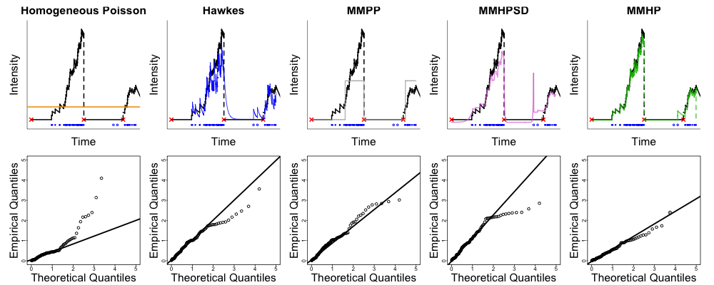
Figure 2: Intensity estimation and Q-Q plots for testing the distribution of rescaled-inter-event times after fitting the five models to synthetic data. Upper panels plot a comparison between intensity functions versus the true intensity, where the blue dots are events, black lines indicate the true intensity function and colored lines are the estimations. Knowing the true intensity, the red crosses are state transitions. Lower panels give Q-Q plots for testing whether the rescaled-inter-event times are distributed as exponential random variables with rate 1.

Case study 2: an application to Williamson et al. (2016) data. Figure 3 shows the intensity estimation and Q-Q plots after fitting the five models to observed event times for the pair of mice shown in Figure 1-(a). MMHP fits the data most reasonably according to the Q-Q plot, whereas the other four models show some indications of lack-of-fit. The fitted homogeneous Poisson process, Hawkes process and MMPP models all show a lighter right tail than the exponential distribution, while the fitted MMHPSD model has a heavier right tail. By using Q-Q plots to examine the distribution of $\{\Lambda_{m}\}_{m=1:M}$, we can compare model fit across competing point process models and can conclude that the MMHP model captures the sporadic and bursty event dynamics of mice social interactions.

Figure 3: Model fit diagnostics for Williamson et al. (2016) data: intensity estimation and Q-Q plots after fitting the five models to real event time data between one pair of mice as shown in Figure 1-(a). Upper panels plot estimated intensity functions after fitting the five models, which are indicated by the black lines. The black dots are the events occurring over time. Lower panels are Q-Q plots to test goodness-of-fit.

3.2 Residual process

According to the Doob-Meyer decomposition theorem (Andersen et al., 2012), given a counting process $N(t)$ with its conditional intensity function $\lambda(t|\mathcal{H}(t))$, the residual process $M(t)$, defined as $M(t)=N(t)-\int_{0}^{t}\lambda(s|\mathcal{H}(s))ds$, is a martingale. Hence, when a point process model is fitted to data and gives an estimated intensity function $\hat{\lambda}(t)$, the raw residual process

$$R(t)=N(t)-\int_{0}^{t}\hat{\lambda}(s)ds$$

can be used to inspect the fit of the model by measuring its discrepancy from 0. Here, we evaluate the raw residual process at the final time point, $T$.

The variance of the above residual process $M(T)$ depends on the intensity function, $\mbox{var}(M(t))=\int_{0}^{t}\lambda(s)ds$. To compare model fit between scenarios with different intensity functions, it is desirable to compute a standardized residual (Baddeley et al., 2005), similar to the Pearson residuals for linear regression. Clements et al. (2011) proposes the Pearson residual process for a counting process as an intensity-weighted version of the raw residual process,

$$\mbox{PR}(t)=\sum_{t_{m}<t}\frac{1}{\sqrt{\lambda(t_{m})}}-\int_{0}^{t}\sqrt{\lambda(s)}ds.$$

Under the true model specification, the variance of $PR(t)$ does not depend on the intensity, i.e., $\mbox{var}(\mbox{PR}(t))=t$ with mean 0 (Clements et al., 2011).

Case study 1: simulated examples. We simulate 50 independent MMHPs with the same parameter settings as in Section 3.1. After fitting Hawkes process, MMPP, MMHPSD and MMHP models to the data, the raw residual $R(T)$ and Pearson residual $\mbox{PR}(T)$ are calculated. Due to the formulation of the Pearson residual process, the integral part cannot be calculated explicitly, and hence, is approximated by numerical integration. Boxplots for 50 raw residuals and Pearson residuals are shown in Figure 4-(a) and (b) separately. We can see that the Hawkes process and MMPP models yield positive residuals most of the time, which means that the models tend to underestimate the intensity. The Hawkes process biased its parameter estimation in order to compromise to the low intensity in state 0, and underestimated the intensity in state 1. The MMPP model cannot capture the volatility of the intensity function in state 1 and yield an underestimated intensity. On the contrary, the MMHPSD model overestimates the intensity, mostly due to its over-sensitive intensity function with the step-wise kernel.

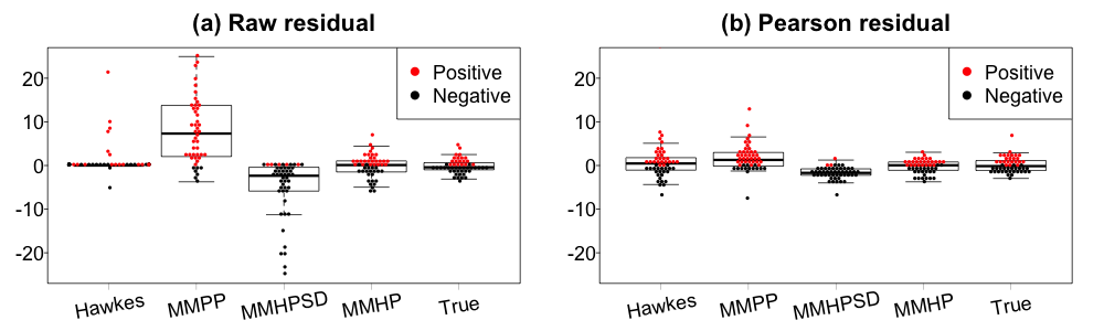
Figure 4: Beeswarm boxplots for raw residual and Pearson residual processes after fitting the four models to synthetic data from 50 independent MMHPs. The residuals calculated from the true intensities are also plotted for comparison.

Case study 2: an application to Williamson et al. (2016) data. Using the data from Williamson et al. (2016), we fit the above four models to all pairs of mice in a cohort separately, and then evaluated the raw residuals and Pearson residuals at final observation time $T$ for all pairs. Figure 5 plots the residuals versus the number of events that occurred between a pair, with smoothing regression lines using LOWESS method (Cleveland, 1979). The MMHP model has residuals closest to 0 and is not sensitive to the number of events (in a sense, the number of events is a rough indicator of intensity) while the other models fail. Comparing the raw residual of the MMPP and MMHPSD models with their Pearson residual, we also observe that the raw residuals have more variability over the number of events. This suggests that the Pearson residual is more appropriate in the network setting, since it is important to have a measurement that is comparable across pairs with varying numbers of pairwise interactions.

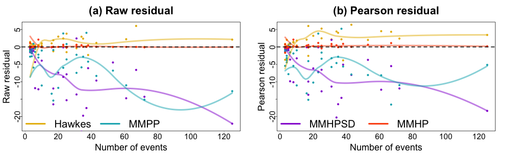
Figure 5: Raw residuals and Pearson residuals after fitting the four models to all pairs in the cohort of mice as in Figure 1-(b) from Williamson et al. (2016). Each model is represented by a different color, with residual values (dots) and a smoothed LOWESS line.

4 Model checking for network heterogeneity and structure

In this section, we provide tools for assessing network point process models. We will focus on MMHP in a network setting and define the marginal intensity for a pair $(i,j)$ as

$$\lambda^{i,j}(t|\mathcal{H}_{V}(t))=\begin{cases}\lambda_{1}^{i,j}+\sum_{t_{m}^{i,j}<t}\alpha^{i,j}e^{-\beta^{i,j}(t-t_{m}^{i,j})},&Z^{i,j}(t)=1\\ \lambda_{0}^{i,j},&Z^{i,j}(t)=0,\end{cases}$$ (1)

where $Z^{i,j}(t)$ is an independent CTMC across all pairs $(i,j)$. We denote the parameters for $(i,j)$ as $\Theta^{i,j}=\{\lambda_{0}^{i,j},\ \lambda_{1}^{i,j},\ \alpha^{i,j},\ \beta^{i,j},\ Q^{i,j}\}$.

4.1 Kolmogorov-Smirnov test

For each pair $(i,j)$, we want to utilize the time rescaling theorem in Section 3.1 and test whether the rescaled-inter-event times, $\{\Lambda^{i,j}_{m}\}_{m=1:M^{i,j}}$ distributed as exponential random variables with rate 1, where $\Lambda^{i,j}_{m}=\int_{t^{i,j}_{m-1}}^{t^{i,j}_{m}}\lambda^{i,j}(s|\mathcal{H}_{V}(s))ds$. To summarize the model fit across pairs in the network, it is important to quantify the test results with a unified measurement. We use the Kolmogorov-Smirnov statistics, $\mbox{KS}^{i,j}=\sup_{x}|\hat{F}^{i,j}(x)-F(x)|$ for each pair $(i,j)$, where $\hat{F}^{i,j}(x)$ is the empirical distribution of the rescaled-inter-event times and $F(x)$ is the cumulative distribution function of the exponential distribution. Larger values of the K-S statistics indicate a larger discrepancy between the model and the network point pattern data.

Case study 1: simultated examples. We simulate network point process data with 10 nodes until time $T=500$ as follows: for each pair $(i,j)$, the marginal intensity $\lambda^{i,j}(s|\mathcal{H}_{V}(s))$ follows (1). All the pairs $(i,j)$ share the same paramters that $\lambda_{0}^{i,j}=0.05,\ \lambda_{1}^{i,j}=0.08,\ \beta^{i,j}=22,\ Q^{i,j}=\bigl{(}\begin{smallmatrix}-0.01&0.01\\ 0.04&-0.04\end{smallmatrix}\bigr{)}$. The matrix $\boldsymbol{\alpha}=[\alpha^{i,j}]_{N\times N}$ is block-structured,

$$\alpha_{ij}=\begin{cases}20,&i,j\in B_{k}\\ 0.5,&i\in B_{k},j\in B_{l},k\neq l\end{cases}.$$

where class $B_{1}=\{1,2,3,4\}$ and $B_{2}=\{5,6,...,10\}$. The total number of events between pair $(i,j)$ until time $T$, $N^{i,j}(T)$ is shown in Figure 6-(a), which has a clear block structure.

We compare the fit of the following two models: (1) across all pairs, the parameter set $\Theta^{i,j}$ shares a same set of values (referred as homogeneous-network model); (2) $\alpha^{i,j}$ varies across pairs such that $\boldsymbol{\alpha}$ has a block structure with the same classes as in the simulation (all other elements of $\Theta^{i,j}$ are the same across all pairs, as in the first model). This is referred to as block-network model.

Figure 6-(b) shows the K-S statistics over the network after fitting the homogeneous-network model to the simulated data, whereas (c) is for the block-network model. Figure 6-(d) displays results from the true intensity function, which has the lowest K-S statistics. Homogeneous-network model (Figure 6 - (b)) fits the data the worst, since it has higher K-S statistics values across network compared to the other models. Figure 6 - (b) also shows a block-structured K-S statistics and demonstrates that the homogeneous-network model performs worse for the between-block pairs, since within-block pairs generate more events and contribute more to the likelihood function.

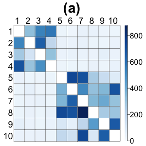
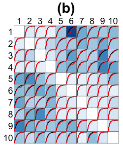
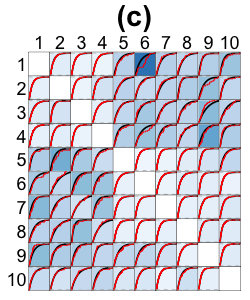
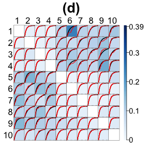
Figure 6: (a) A heatmap of simulated network point process data: the total number of events occurred between each pair. (b)(c) Matrices of K-S statistics after fitting homogeneous and block-network models to the simulated data in (a). The rows and columns of each matrix correspond to senders and receivers, respectively. Color shades reflect the values of the K-S test statistics. (d) Matrix of K-S statistics calculated from true intensity function.

Case study 2: an application to Williamson et al. (2016) data. For the interaction event times among a group of mice as shown in Figure 1-(b), we fit the following two models: (1) the parameter set $\Theta^{i,j}$ for MMHP is the same across pairs (referred as homogeneous-network model); (2) $\Theta^{i,j}$ is allowed to vary freely across pairs (referred as heterogeneous-network model). Figure 7 plots the matrices of K-S statistics after fitting the above two models. Since the heterogeneous-network model has more flexibility across pairs and can adapt well on various pairs’ dynamics, its K-S statistics are smaller and the model fits the data better. Especially for the pair $(7,5)$, they started engaging in interactions during the last period of observations, which sets them apart from the other pairs, as shown in 1-(b). The homogeneous-network model fits this pair poorly, whereas the heterogeneous-network model better captures this pattern.

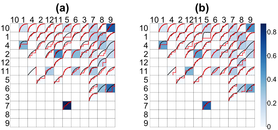
Figure 7: Matrices of K-S statistics after fitting homogeneous-network model (in (a)) and heterogeneous-network model (in (b)) to the mice interaction data. Color shades reflects the values of the K-S test statistics.

4.2 Structure score based on Pearson residual matrix

The Pearson residual is more valuable for diagnosing model fit in the network setting, since it is comparable across pairs and not influenced by intensity function. For a pair $(i,j)$, the Pearson residual is

$$\mbox{PR}_{i,j}(T)=\sum_{t^{i,j}_{m}}\frac{1}{\sqrt{\hat{\lambda}^{i,j}(t^{i,j}_{m})}}-\int_{0}^{T}\sqrt{\hat{\lambda}^{i,j}(s)}ds.$$

To assess model fit, we propose to quantify the network structure in the Pearson residual matrix, $\mbox{PR}:=[\mbox{PR}_{i,j}]_{N\times N}$. In order to spot systematic overestimation or underestimation issues, we separate the Pearson residual matrix into two matrices for the positive and negative residual values respectively. We preserve the positive residuals in the underestimation matrix $\mbox{PR}^{+}$, such that $\mbox{PR}^{+}_{i,j}=\mbox{PR}_{i,j}$ if $\mbox{PR}_{i,j}>0$ and $\mbox{PR}^{+}_{i,j}=0$ otherwise. Similarly, we create the overestimation matrix $\mbox{PR}^{-}$ using the absolute values of negative residuals. We conduct nonnegative matrix factorization (NMF) (Lee and Seung, 2001) on each of the matrices, $A\approx WH$, where $A\in\mathbb{R}^{N\times N}$ is $\mbox{PR}^{+}$ or $\mbox{PR}^{-}$ and $W\in\mathbb{R}^{N\times K},H\in\mathbb{R}^{K\times N}$. $K$ is usually set to be much smaller than $N$, so that $WH$ is a lower-rank approximation of $A$. We introduce a matrix structure score as $\frac{||A-WH||_{F}}{||A||_{F}}$, where $||\cdot||_{F}$ is the matrix Frobenius norm. If NMF can recover the residual matrix well, the score is larger, suggesting that the model fits the data worse and yields a more structured residual matrix.

Case study 1: simulated examples. Using simulated data as in Section 4.1, we calculate the Pearson residual matrix after fitting the homogeneous and block-network models and plot them in Figure 8-(a) and (b) respectively. For a better comparison, we also use the true model intensity to calculate the residuals and plot in Figure 8-(c). Table 1 compares the matrix structure score of the underestimation $\mbox{PR}^{+}$ and overestimation matrix $\mbox{PR}^{-}$ across models by using $K=2$. The homogeneous model exhibits larger positive residuals within-block. This demonstrates that the estimation of the intensities for within-block pairs are biased towards lower values because the model is network-homogeneous and not adequate to capture intense interactions of within-block pairs. The matrix structure score of this model is higher in both overestimation and underestimation matrices as shown in Table 1, which is a quantified validation for its lack-of-fit.

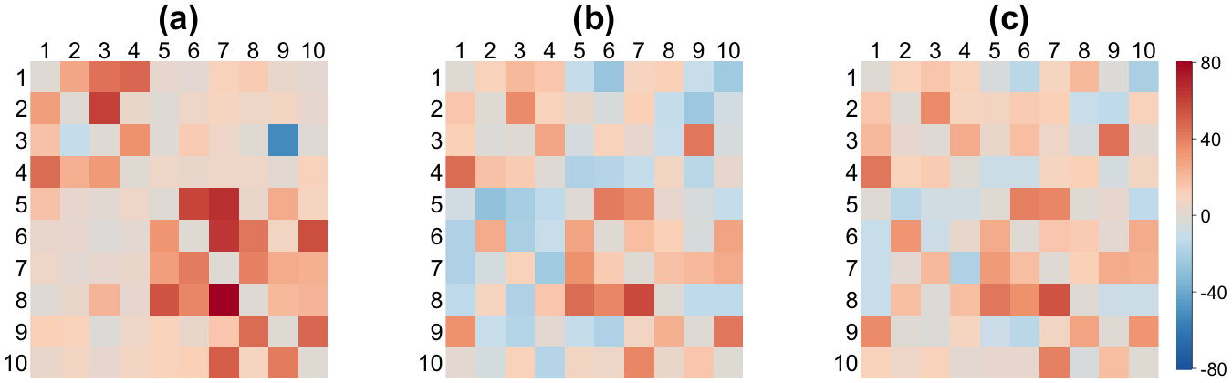
Figure 8: Matrices of the Pearson residuals after fitting models to simulated data. (a)(b) are results after fitting the homogeneous and block-network models to the simulated data. (c) is from the true model that is used to generate simulation. Red colors represent positive residuals, indicating that the model underestimates the intensity function, whereas blue colors represent negative residuals and hence overestimation.

homogeneous block true positive 0.46 0.41 0.41 negative 0.93 0.43 0.36 Table 1: Structure scores for simulated examples.

homogeneous heterogeneous positive 0.79 0.69 negative 0.77 0.55 Table 2: Structure scores for the Williamson et al. (2016) example.

Case study 2: an application to Williamson et al. (2016) data. Figure 9 shows the Pearson residual matrix after fitting homogeneous and heterogeneous-network models to the mice interaction data. The models’ assumptions are defined in Section 4.1. The homogeneous-network model tends to overestimate the intensity function when individual 4 and 11 are the senders, because the inference is biased by a large number of interactions initiated by active individuals. Thus, this pattern in the residual matrix yields a larger matrix structure score, especially for the negative residuals, as shown in Table 2, where $K$ is set to be 2. It suggests that the homogeneous-network model is not adequate to capture the network dynamics, while the heterogeneous-network model has more flexibility and is superior in terms of Pearson residual and structure score.

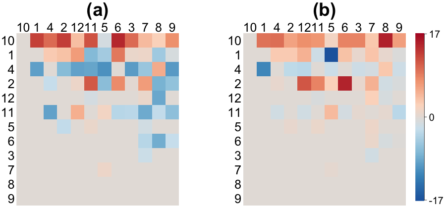
Figure 9: Matrices of the Pearson residuals after fitting models to Williamson et al. (2016) data. (a) is for homogeneous-network model and (b) is for heterogeneous-network model. The rows and columns of all matrices are reordered by the I&SI dominance rank.

5 Summary

In this paper, we propose diagnostic statistics and visualization tools for network point process models. The evaluation techniques are theoretically well-grounded and can be applied to intensity-based models for network point pattern data generally. We use simulations and real data examples to demonstrate the utility of our approaches. By inspecting lack-of-fit in terms of both temporal dependence and network structures, the proposed suite of diagnostic statistics and visualizations can reveal deficiencies in network point process models and provide important insights that can lead to model improvements.

6 Acknowledgment

This material is based on research sponsored by DARPA agreement number D17AC00001. The content of the information does not necessarily reflect the position or the policy of the Government, and no official endorsement should be inferred.

References

- Andersen et al. [2012] P. K. Andersen, O. Borgan, R. D. Gill, and N. Keiding. Statistical models based on counting processes. Springer Science & Business Media, 2012.
- Baddeley et al. [2005] A. Baddeley, R. Turner, J. Møller, and M. Hazelton. Residual analysis for spatial point processes (with discussion). Journal of the Royal Statistical Society: Series B (Statistical Methodology), 67(5):617–666, 2005.
- Barabasi [2005] A.-L. Barabasi. The origin of bursts and heavy tails in human dynamics. Nature, 435(7039):207–211, 2005.
- Brown et al. [2002] E. N. Brown, R. Barbieri, V. Ventura, R. E. Kass, and L. M. Frank. The time-rescaling theorem and its application to neural spike train data analysis. Neural computation, 14(2):325–346, 2002.
- Clements et al. [2011] R. A. Clements, F. P. Schoenberg, and D. Schorlemmer. Residual analysis methods for space-time point processes with applications to earthquake forecast models in california. The Annals of Applied Statistics, pages 2549–2571, 2011.
- Cleveland [1979] W. S. Cleveland. Robust locally weighted regression and smoothing scatterplots. Journal of the American statistical association, 74(368):829–836, 1979.
- Cox and Lewis [1972] D. R. Cox and P. A. W. Lewis. Multivariate point processes. In Proc. 6th Berkeley Symp. Math. Statist. Prob, volume 3, pages 401–448, 1972.
- Daley and Vere-Jones [2003] D. J. Daley and D. Vere-Jones. An introduction to the theory of point processes: volume I: elementary theory and methods. Springer Science & Business Media, 2003.
- Fan and Shelton [2009] Y. Fan and C. R. Shelton. Learning continuous-time social network dynamics. In Proceedings of the Twenty-Fifth Conference on Uncertainty in Artificial Intelligence, pages 161–168. AUAI Press, 2009.
- Fischer and Meier-Hellstern [1993] W. Fischer and K. Meier-Hellstern. The Markov-modulated Poisson process (MMPP) cookbook. Performance evaluation, 18(2):149–171, 1993.
- Hawkes [1971] A. G. Hawkes. Spectra of some self-exciting and mutually exciting point processes. Biometrika, pages 83–90, 1971.
- Lee and Seung [2001] D. D. Lee and H. S. Seung. Algorithms for non-negative matrix factorization. In Advances in neural information processing systems, pages 556–562, 2001.
- Lewis and Shedler [1979] P. W. Lewis and G. S. Shedler. Simulation of nonhomogeneous poisson processes by thinning. Naval research logistics quarterly, 26(3):403–413, 1979.
- Linderman and Adams [2014] S. Linderman and R. Adams. Discovering latent network structure in point process data. In International Conference on Machine Learning, pages 1413–1421, 2014.
- Perry and Wolfe [2013] P. O. Perry and P. J. Wolfe. Point process modelling for directed interaction networks. Journal of the Royal Statistical Society: Series B (Statistical Methodology), 75(5):821–849, 2013.
- Rabiner [1989] L. R. Rabiner. A tutorial on hidden markov models and selected applications in speech recognition. Proceedings of the IEEE, 77(2):257–286, 1989.
- Saito et al. [2009] K. Saito, M. Kimura, K. Ohara, and H. Motoda. Learning continuous-time information diffusion model for social behavioral data analysis. In Asian Conference on Machine Learning, pages 322–337. Springer, 2009.
- Schmid and de Vries [2013] V. S. Schmid and H. de Vries. Finding a dominance order most consistent with a linear hierarchy: an improved algorithm for the i&si method. Animal Behaviour, 86(5):1097–1105, 2013.
- Wang et al. [2012] T. Wang, M. Bebbington, and D. Harte. Markov-modulated Hawkes process with stepwise decay. Annals of the Institute of Statistical Mathematics, 64(3):521–544, 2012.
- Williamson et al. [2016] C. M. Williamson, W. Lee, and J. P. Curley. Temporal dynamics of social hierarchy formation and maintenance in male mice. Animal Behaviour, 115:259–272, 2016.
- Wu et al. [2019] J. Wu, T. Zheng, and J. Curley. Markov-modulated Hawkes processes for sporadic and bursty event occurrences. arXiv: 1903.03223, 2019.
- Yang et al. [2017] J. Yang, V. Rao, and J. Neville. Decoupling homophily and reciprocity with latent space network models. In UAI, 2017.
- Zipkin et al. [2016] J. R. Zipkin, F. P. Schoenberg, K. Coronges, and A. L. Bertozzi. Point-process models of social network interactions: Parameter estimation and missing data recovery. European Journal of Applied Mathematics, 27(3):502–529, 2016.