Influence of equilibrium and nonequilibrium environments on macroscopic realism through the Leggett-Garg inequalities

Abstract

We study the macroscopic realism (macrorealism) through the two- and three-time Leggett-Garg inequalities (LGIs) in a two interacting qubits system. The two qubits are coupled either with two bosonic (thermal or photonic) baths or fermionic (electronic) baths. We study both how the equilibrium and nonequilibrium environments influence the LGIs. One way to characterize the nonequilibrium condition is by the temperature difference (for the bosonic bath) or the chemical potential difference (for the fermionic bath). We also study the heat or particle current and the entropy production rate generated by the nonequilibrium environments. Analytical forms of LGIs and the maximal value of LGIs based on the quantum master equation beyond the secular approximation are derived. The LGI functions and the corresponding maximal value have separated contributions, the part describing the coherent evolution and the part describing the coupling between the system and environments. The environment-coupling part can be from the equilibrium environment or the nonequilibrium environment. The nonequilibrium dynamics is quantified by the Bloch-Redfield equation which is beyond the Lindblad form. We found that the nonequilibriumness quantified by the temperature difference or the chemical potential difference can lead to the LGIs violations or the increase of the maximal value of LGIs, restoring the quantum nature from certain equilibrium cases where LGIs are preserved. The corresponding nonequilibrium thermodynamic cost is quantified by the nonzero entropy production rate. The violation enhancement increases with the increase of the entropy production rate under certain nonequilibrium conditions. Therefore, the LGIs violation enhancement can be realized by the thermodynamic nonequilibrium cost. Our results shed light on the nature of the macrorealism and the relationship between the nonequilibriumness and the quantum temporal correlation. Our finding of the nonequilibrium promoted LGIs violations suggests a new strategy for the design of quantum information processing and quantum computational devices to maintain the quantum nature and quantum correlations for long.

I Introduction

Quantum correlations, which distinguish the quantum world from the classical world, not only are rooted in the fundamental nature of quantum mechanics, but also become valuable resources for quantum information processing tasks Nielsen and Chuang (2010). The spatial quantum correlations, known as the entanglement Horodecki et al. (2009) or the discord Modi et al. (2012), show perhaps the most spooky phenomenon in the nature. The well-known Bell inequalities Bell (1964) were proposed in 1964 to distinguish the classical correlations with the quantum ones, and the violation is inconsistent with the local hidden variable theory (the classical correlation). The genuine nonlocality, also called Bell nonlocality (violation of Bell inequalities), has been demonstrated in many experiments since 1972 Freedman and Clauser (1972); Hensen et al. (2015); Brunner et al. (2014).

The temporal quantum correlations, generated by sequential non-commuting measurements on a single system at different times, is also different from the classical probabilistic descriptions. Such a discrepancy (between the classical and the quantum) on temporal correlations can be distinguished by the correlation inequalities called Leggett-Garg inequalities (LGIs) Leggett and Garg (1985); Emary et al. (2013). LGIs are temporal analog version of Bell inequalities. Bell inequalities and LGIs have the same spirit: the joint probability distribution can not be assigned to all measurement results, regardless if the measurements are performed on the separated space or time Markiewicz et al. (2014). LGIs were firstly motivated to demonstrate the macroscopic coherence, namely how to justify the existence of the macroscopic superposition state. LGIs test the realism of physical states: the system is in definite states with distinct observable values, which is also the essence of the hidden variable theory. Violation of LGIs implies that the system is undergoing the quantum mechanical time evolution which is beyond the classical probabilistic description.

Although Bell inequalities and LGIs share the same spirit, Fine’s theorem Fine (1982) can not be applied to the original LGIs, since LGIs require measuring the noncommuting observables at different times and the no-signaling condition fails. LGIs are only the sufficient condition (not the necessary condition) for testing the macrorealism Clemente and Kofler (2016). There are different proposals to bring the no-signaling condition in testing the macrorealism for suggesting the sufficient and necessary condition. For examples, the no-signaling in time condition Kofler and Brukner (2013) has a direct analogy to the no-signaling condition in Bell inequalities. Variants of LGIs, such as the Wigner’s form of LGIs Saha et al. (2015) and the augmented set of LGIs Halliwell (2016), can also remedy the sufficient condition issue. Halliwell recently showed that these necessary and sufficient conditions are not equivalent, instead they are testing different degrees (notions) of the macrorealism Halliwell (2017, 2019).

Although the LGIs are devoted to demonstrate the macroscopic coherence, the violation of LGIs can be attributed from the violation of the macrorealism description or/and the violation of the noninvasive measurability (NIM) Emary et al. (2013). There have been intensive theoretical and experimental studies on how to achieve the NIM to demonstrate the violation of the macrorealism assumption. There are four major strategies to exclude the invasive measurement issue. First, the NIM assumption, in some circumstances, can be replaced by the stationary assumption Huelga et al. (1995, 1996) (see the experiments based on the stationary assumption Waldherr et al. (2011); Zhou et al. (2015); Formaggio et al. (2016)). Second, experiments can be performed by the weak measurement to diminish the effects of measurements on the system Van Der Wal et al. (2000); Palacios-Laloy et al. (2010); Goggin et al. (2011). Third, the original LGIs argued that the ideal negative measurement (INM) in principle can detect the system without disturbing it Leggett and Garg (1985). The quantum version of the INM has been realized in many experiments Knee et al. (2012); Katiyar et al. (2013, 2017); Majidy et al. (2019). Wilde and Mizel almost closed the loophole by designing the control experiments to show that the violation of LGIs does not come from the invasive measurements Wilde and Mizel (2012) (see the experiments Knee et al. (2016)).

Quantum coherence is the reason why the macrorealism notion has to be rejected. However, quantum coherence is notoriously fragile due to the coupling with the environments. This leads to the decoherence Leggett et al. (1987); Breuer and Petruccione (2002); Zurek (2003). Decoherence has to be included when studying the violation of LGIs in the real world. When the system is coupled with the environments (also called reservoirs or baths in this paper), the dynamics between the system and the environments can be classified as Markovian (memoryless) Breuer and Petruccione (2002); Scully and Zubairy (1999) or non-Markovian (with the memory effect) De Vega and Alonso (2017). Both Markovian Emary (2013); Chen et al. (2013); Łobejko et al. (2015); Friedenberger and Lutz (2017); Chanda et al. (2018); Castillo et al. (2013) and non-Markovian Chen and Ali (2014); Datta et al. (2018) effects on violations of LGIs have been studied before. The non-Markovian case requires special care since the quantum coherent evolution can be rewritten as a non-Markovian rate equation which can violate the LGIs Emary et al. (2013); Lambert et al. (2010).

The effects of the environments to the system can be classified as equilibrium and nonequilibrium, where the nonequilibrium condition is quantified as the temperature difference or the chemical potential difference of the environments or baths. The nonequilibrium condition represents the degree of the energy or matter exchange between the system and the reservoirs, respectively. Coherence Addis et al. (2014); Zhang et al. (2015); Guarnieri et al. (2018) or entanglement Plenio et al. (1999); Arnesen et al. (2001); Wang (2001); Kamta and Starace (2002); Braun (2002); Benatti et al. (2003); Verstraete et al. (2009); Zhao et al. (2011); Huelga et al. (2012) generated and controlled from the equilibrium environment has been intensely studied in last 20 years, due to their potential applications in the quantum information processing. Nonequilibrium environments Esposito et al. (2009) draw more attentions in recent years. Nonequilibrium environments have their own significance for maintaining and enhancing the long time coherence Zhang and Wang (2014); Li et al. (2015); Wang et al. (2018) or entanglement Lambert et al. (2007); Quiroga et al. (2007); Sinaysky et al. (2008); Wu and Segal (2011); Liao et al. (2011); Dhar et al. (2012); Bellomo and Antezza (2013); Zhang and Wang (2015); Wang et al. (2019); Tavakoli et al. (2018); Tacchino et al. (2018); Wang and Wang (2019). At the equilibrium scenario, coupling with the environment has only negative influence on the violations of LGIs Chen et al. (2013); Łobejko et al. (2015); Friedenberger and Lutz (2017). However, the steady-state coherence generated under the nonequilibrium condition Zhang and Wang (2014); Li et al. (2015); Wang et al. (2018) seems to suggest that the nonequilibriumness may contribute to or enhance the violations of LGIs. Only very limited numbers of studies have been devoted to the issue of how the nonequilibriumness (the energy or particle exchange with the system) influences the quantum dynamical nature of the system Castillo et al. (2013); Mendoza-Arenas et al. (2019).

To address the question on how equilibrium and nonequilibrium environments influence the LGIs, we study the following setup: the two-coupled-qubit system (may have different frequencies) immersed into two individual reservoirs respectively. The two reservoirs can have the same or different temperatures (bosonic baths) or chemical potentials (fermionic baths). The weak coupling between the system and the environments and the Markovian dynamics are assumed in the model. The dynamics of the system is described by the Bloch-Redfield equation Bloch (1957); Redfield (1957), without the secular approximation made in the Lindblad equation. The Lindblad equation is not used here because the nonequilibrium steady state coherence is neglected by the secular approximation in the Lindblad equation Zhang and Wang (2014); Li et al. (2015); Wang et al. (2018); Guarnieri et al. (2018); Wang et al. (2019). Specifically, if the secular approximation has been applied, the population space and the coherent space will be decoupled. Moreover, the LGIs are dependent on the local observables (local measurements performed on one qubit). Furthermore, if the secular approximation is applied, LGIs will have the symmetric response to the nonequilibrium environments Castillo et al. (2013). However, the Bloch-Redfield equation is criticized by non-positivity of the density matrix evolution in certain parameter regimes. The positivity of Bloch-Redfield equation may be recovered by the initial conditions Suárez et al. (1992) or further approximations Jeske et al. (2015); Farina and Giovannetti (2019). The validity of Bloch-Redfield equation is beyond the scope of the study in this paper. Instead, we circumvent the positivity issue by concentrating on the parameter regimes which give the positive density matrix.

In our study, we consider the equilibrium and nonequilibrium steady state as the initial state for the LGIs. Therefore, only the time interval of sequential measurements matters. We adopt the augmented LGIs (a set of two- and three-time LGIs) as the necessary and sufficient condition for the macrorealism. We give analytical results about the steady state at both equilibrium and nonequilibrium scenarios. In nonequilibrium case, the two reservoirs are sustained with a constant temperature difference or chemical potential difference if the two baths are bosonic or fermionic, respectively. Sequentially measuring one local qubit gives the temporal correlations of the local observable. We analytically find the augmented set of LGIs based on the weak-coupling assumption. We approximate the augmented set of LGIs up to the first order coupling strength between the system and the environments. The zeroth order (in terms of the coupling strength) can be viewed as the coherent evolution part and the first-order part describes the effects on LGIs from the dynamical coupling between the system and the environments. The steady-state coherence in the energy basis, which is only nonzero in the nonequilibrium setups, has the contribution to the two-time LGI functions. However, such contribution is not significant enough for the violation of two-time LGIs. Therefore, we concentrate on the three-time LGIs (the original proposed LGIs) in our study. The maximum of LGI (MLGI) functions can be used to quantify the degree of the LGIs violations.

In the equilibrium cases, the MLGI function has the non-monotonic relation with the common temperature or the chemical potential. In the low temperature regime, increasing the temperature can increase the population of the excited states, which are superposition of local states. In the high temperature regime, increasing the temperature leads to a stronger thermal effect (decoherence). In the nonequilibrium scenario, the MLGI function can be enhanced by the nonequilibrium conditions: the temperature difference or the entropy production rate in the bosonic environments; the chemical potential difference or the entropy production rate in the fermionic environments. The LGIs violation enhancement has a thermodynamic cost quantified by the nonzero entropy production rate. The bosonic enhancement is only realized at the low mean temperature regime. If we choose to measure the qubit 1, then the MLGI function has greater enhancement if the qubit 1 is coupled with the lower temperature bath. Note that the Lindblad gives symmetric results: the qubit 1 coupled with the bath with a lower temperature $T_{1}$ and the qubit 2 coupled with the bath with a higher temperature $T_{2}$ gives the same result when the qubit 1 is coupled with the bath with a higher temperature $T_{2}$ and the qubit 2 is coupled with the bath with a lower temperature $T_{1}$. In other words, the Lindblad does not characterize well the nonequilibrium dynamics. We obtained the MLGI function enhancement from the chemical potential difference (fermionic baths) when the mean chemical potential is away from the resonant point. The resonance occurs when the mean chemical potential equals to the mean energy of the two-qubit system. We have also studied the LGIs violations when the two-qubit system has detuned energy splitting. We got a larger MLGI function (than the equilibrium case) when the low-frequency qubit is coupled with the high-temperature bath or high chemical potential bath and the high-frequency qubit is coupled with the low-temperature bath or high chemical potential. Although the model in our study is far from macroscopic, the results suggest that the nonequilibrium environments may be beneficial to the real macroscopic coherence.

The rest of the paper is organized as follows. Section II reviews the time correlation functions and the two- and three-time LGIs. We also briefly review how the ideal negative measurement (as the noninvasive measurement) can be realized on the qubit system. Section III presents the dynamic quantum master equation of the system and the analytical form of the steady state. We study the LGI functions and MLGI function given by the system coupled with the equilibrium and nonequilibrium environments in Secs. IV and V respectively. The results are based on analytical expressions and are demonstrated numerically. The last section gives the conclusion. The detailed expressions for the Bloch-Redfield equation and the heat or particle current are presented in the Appendix.

II The two- and three-time Leggett-Garg inequalities

II.1 The correlation function

In classical probabilistic theory, the results of measurements performed at different times $t_{j}$ and $t_{l}$ can be described by the joint probability $P(Q_{j},t_{j};Q_{l},t_{l})$. Here $Q_{j}$ is the measurement value at $t_{j}$. The correlation function characterizing the measurement results at $t_{j}$ and $t_{l}$ is defined as

$$C_{\text{cl}}(t_{j},t_{l})=\sum_{Q_{j},Q_{l}}Q_{j}Q_{l}P(Q_{j},t_{j};Q_{l},t_{l})$$ (1)

The subscript “cl” distinguishes the correlation functions from the quantum case.

In the quantum mechanical description, there is no unique analog of classical correlation function defined in (1), because of the operator ordering. We can define the quantum correlation function in the perspective of the measurement results. Suppose we have dichotomic observables

$$\hat{Q}=\sum_{m}a_{m}\hat{\Pi}_{m}$$ (2)

with $a_{m}=\pm 1$. Operators $\hat{\Pi}_{m}$ are the corresponding projections. Since we only consider the quantum cases, we omit the hat notation on the operator for simplicity. Suppose that the system has the time evolution

$$\frac{d\rho}{dt}=\mathcal{W}\rho$$ (3)

where $\mathcal{W}$ is the superoperator generating the dynamics. Note that we do not restrict ourselves in the unitary evolution only. Based on the perspective of the classical measurement values, the correlation function in the quantum case has the form

$$C_{\text{q}}(t_{j},t_{l})= \sum_{m,n}a_{m}a_{n}\mathrm{Tr}\left(\Pi_{m}e^{\mathcal{W}(t_{j}-t_{l})}\left(\Pi_{n}\rho(t_{l})\Pi_{n}\right)\right)$$

$$= \mathrm{Tr}\left(Q(t_{j})\left(\sum_{n}a_{n}\Pi_{n}\rho(t_{l})\Pi_{n}\right)\right)$$ (4)

The subscript q means quantum. Here, the operator $Q(t_{j})$ is defined in the Heisenberg picture. The correlation function $C_{\text{q}}(t_{j},t_{l})$ has the same interpretation as the classical correlation $C_{\text{cl}}(t_{j},t_{l})$ in Eq. (1).

Studies regarding the LGIs usually take the other form of the quantum correlation function Emary et al. (2013):

$$C^{\prime}_{\text{q}}(t_{j},t_{l})= \frac{1}{2}\mathrm{Tr}\left(\left\{Q(t_{j}),Q(t_{l})\right\}\rho(t_{l})\right)$$

$$= \mathrm{Tr}\left(Q(t_{j})\frac{1}{2}\left\{Q(t_{l}),\rho(t_{l})\right\}\right)$$ (5)

which is also the real part of the “naive” quantum correlation function

$$C^{\prime\prime}_{\text{q}}(t_{j},t_{l})=\mathrm{Tr}(Q(t_{j})Q(t_{l})\rho(t_{l}))$$ (6)

The quantum correlation function $C^{\prime\prime}_{\text{q}}(t_{j},t_{l})$ is in general a complex function. The imaginary part of it is a measure of noncommutativity for observables $Q(t_{j})$ and $Q(t_{l})$ (without classical analog).

Note that the anticommutator in Eq. (II.1) has the explicit form

$$\frac{1}{2}\left\{Q(t_{l}),\rho(t_{l})\right\}\\ =\sum_{n}a_{n}\Pi_{n}\rho(t_{l})\Pi_{n}+\frac{1}{2}\sum_{n\neq n^{\prime}}(a_{n}+a_{n^{\prime}})\Pi_{n}\rho(t_{l})\Pi_{n^{\prime}}$$ (7)

Since we set that $a_{n}=\pm 1$, the second term in the above equation is zero. If we substitute the above expression into Eq. (II.1) (with the setting $a_{n}=\pm 1$), then the correlation function $C_{\text{q}}(t_{j},t_{l})$ in Eq. (II.1) has the same form of $C^{\prime}_{\text{q}}(t_{j},t_{l})$ in Eq. (II.1). Based on the setting $a_{n}=\pm 1$, we reach the conclusion that the commonly used quantum correlation function $C^{\prime}_{\text{q}}(t_{j},t_{l})$ in Eq. (II.1) has the same interpretation with the classical correlation $C_{\text{cl}}(t_{j},t_{l})$ in Eq. (1). Note that such interpretation is only valid with the dichotomic observables with eigenvalues $\pm 1$. Some literatures using the measurement values $0,1$ Huelga et al. (1996); Waldherr et al. (2011) do not have such interpretation.

II.2 The three-time Leggett-Garg inequalities

Originated from the macrorealism test, the original LGIs are based on the following assumptions:

1. Macrorealism per se: the physical object is in one of the distinct states at any time.

2. NIM: it is in principle possible to reveal the state of the object without disturbing the following dynamics.

3. Induction: the present state can not be affected by the future measurements.

The induction assumption is also assumed. The NIM assumption is based on the macrorealism per se assumption. Quantum systems do not admit either macrorealism per se assumption or the NIM assumption. However, a macrorealist can always claim that the violation of LGIs is from the failure to perform the NIM. This is the “clumsiness loophole” in testing the macrorealism. Although the loophole free test is not proposed yet, multiple different strategies have been suggested to exclude the violation of the NIM assumption (see the review Emary et al. (2013) for more comments). Nevertheless, the aim of this paper is not to address the NIM assumption in the macrorealism tests. Instead, we assume that the INM protocol can always be perfectly realized. How to realize the INM in the quantum system is briefly reviewed in Sec. II.4. Then, we focus on the influence of the equilibrium and nonequilibrium environments on the violations of LGIs.

The essence of deriving the LGIs is to assign the probability distribution over the three-time measurements $P(Q_{3},t_{3};Q_{2},t_{2};Q_{1},t_{1})$. Then, the two-time probability $P(Q_{j},t_{j};Q_{l},t_{l})$ can be obtained from the marginal of the three-time probability. Then, the two-time correlations are bounded by the following inequalities Leggett and Garg (1985)

$$C_{\text{cl}}(t_{1},t_{2})+C_{\text{cl}}(t_{2},t_{3})-C_{\text{cl}}(t_{1},t_{3})\leq 1$$ (8a)

$$C_{\text{cl}}(t_{1},t_{2})-C_{\text{cl}}(t_{2},t_{3})+C_{\text{cl}}(t_{1},t_{3})\leq 1$$ (8b)

$$- C_{\text{cl}}(t_{1},t_{2})-C_{\text{cl}}(t_{2},t_{3})-C_{\text{cl}}(t_{1},t_{3})\leq 1$$ (8c)

$$- C_{\text{cl}}(t_{1},t_{2})+C_{\text{cl}}(t_{2},t_{3})+C_{\text{cl}}(t_{1},t_{3})\leq 1$$ (8d)

The above inequalities only concern the constraints on the two-time probability distribution given by the three-time probability distribution. The three-time LGIs can be generalized to the multi-time cases Emary et al. (2013). If the initial time is irrelevant, then the correlation function only depends on the time interval. In practice, we can keep the two-time intervals in the three-time measurements to be the same, i.e., $t_{2}-t_{1}=t_{3}-t_{2}=t$. Then, the four LGIs in Eqs. (8a)-(8d) can be reduced into two inequalities

$$\pm 2C_{\text{cl}}(t)-C_{\text{cl}}(2t)\leq 1\\$$ (9)

where $C_{\text{cl}}(t)=C_{\text{cl}}(t_{1},t_{2})=C_{\text{cl}}(t_{2},t_{3})$ and $C_{\text{cl}}(2t)=C_{\text{cl}}(t_{1},t_{3})$.

Since quantum mechanics rejects either the microrealism or the macrorealism, the quantum correlation functions do not satisfy the inequalities (9). We define the corresponding three-time LGI functions

$$\mathcal{I}_{\pm}(t,\rho^{\text{ss}})=\pm 2C_{\text{q}}(t)-C_{\text{q}}(2t)$$ (10)

where the quantum correlation function $C_{\text{q}}(t)$ is given by Eq. (II.1) or Eq. (II.1). Note that the functions $\mathcal{I}_{\pm}(t,\rho^{\text{ss}})$ depend on the initial density matrix $\rho^{\text{ss}}$ and the equal interval time $t$ once the dichotomic observable $Q$ is fixed. Here, the superscript “ss” in $\rho^{\text{ss}}$ represents the steady state of the system (therefore, the initial time is irrelevant). The LGI functions $\mathcal{I}_{\pm}(t,\rho^{\text{ss}})$ can break the classical bound but are limited with the value Emary et al. (2013):

$$\mathcal{I}_{\pm}(t,\rho^{\text{ss}})\leq\frac{3}{2}$$ (11)

Only the evolution defined in Eq. (3) is unitary, the LGI functions $\mathcal{I}_{\text{a,b}}(t,\rho^{\text{ss}})$ can be saturated.

II.3 The two-time Leggett-Garg inequalities

The original three-time LGIs are only the sufficient condition for testing the macrorealism Clemente and Kofler (2016). There are several different proposals for the necessary and sufficient conditions Kofler and Brukner (2013); Saha et al. (2015); Halliwell (2016). Different proposals are not exactly equivalent Halliwell (2017, 2019). Here we follow a approach which remains closely with the original three-time LGIs. A new set of two-time LGIs combined with the three-time LGIs in Eqs. (8a)-(8d) form the necessary and sufficient condition Halliwell (2016, 2017, 2019).

Since both the single-time probability and the two-time probability distributions can be obtained from the marginals of the three-time probability, the averages and the two-time correlation functions also satisfy the inequalities

$$-a_{j}\langle Q(t_{j})\rangle-a_{l}\langle Q(t_{l})\rangle-a_{j}a_{l}C_{\text{cl}}(t_{j},t_{l})\leq 1$$ (12)

where $a_{j},a_{l}=\pm 1$. Here, the time pair $(j,l)$ takes the values $(1,2),(2,3),(1,3)$. Therefore, there are 12 inequalities in total. The averages and the correlation functions can be measured in three different experiments. The averages do not have the invasive measurement issue since only one measurement is performed. Similar with the three-time LGIs, we assume that the correlation function $C_{\text{cl}}(t_{j},t_{l})$ satisfies the NIM assumption. Note that the inequalities in Eq. (12) are the necessary and sufficient conditions for the macrorealism in the two-time level. In other words, if the two-time inequalities are satisfied, there are no contradictions between the joint probability $P(Q_{j},t_{j};Q_{l},t_{l})$ and the single-time probability $P(Q_{j},t_{j})$. Based on a simpler proof of Fine’s theorem Halliwell (2014), Halliwell showed that if the three-time LGIs in Eqs. (8a)-(8d) combined with the two-time LGIs in Eq. (12) are satisfied, the three-time joint probability can always be constructed, therefore giving the necessary condition for the macrorealism.

If the system reaches the steady state, the initial time is not concerned and the correlation function only depends on the time interval between the two measurements. Surprisingly, only 2 of the 12 inequalities are nontrivial and the two remaining inequalities have the unified form

$$2\langle Q\rangle_{\text{ss}}-C_{\text{cl}}(t)\leq 1$$ (13)

We define the corresponding two-time LGI function with the steady state condition:

$$\mathcal{I}_{2}(t,\rho^{\text{ss}})=2\langle Q\rangle_{\text{ss}}-C_{\text{q}}(t)$$ (14)

where the quantum correlation function $C_{\text{q}}(t)$ is given by Eq. (II.1) or Eq. (II.1). Instead of the classical bound shown in Eq. (13), the two-time LGI function is bounded by

$$\mathcal{I}_{2}(t,\rho^{\text{ss}})\leq 3$$ (15)

See examples in Sec. IV. Recent experiments on nuclear spins showed that different initial states can separately violate either the three-time LGIs or the two-time LGIs Majidy et al. (2019).

II.4 The ideal negative measurements

Figure 1: The quantum INM based on the classical INM protocol. The CNOT and anti-CNOT gates are defined in Eqs. (16a) and (16b), respectively. The measurement results are discarded of the ancilla qubit $|0\rangle\langle 0|$ is flipped. The evolution of the density matrix is described by the superoperator $\mathcal{W}$ defined in (3).

To demonstrate the violation of the macrorealism assumption via the two-time and three-time LGIs, the experiments performed need to rule out the possibility that the violations of LGIs do not come from the invasive measurements. Leggett and Garg originally argued that the noninvasive measurement can always be applied via the INM Leggett and Garg (1985). Suppose that the measurement apparatus only clicks (interacting with the system) when the system is at the state assigned with the value $1$. Therefore, if the measurement device remains unclicked, we can learn that the system stays at the state with the assigned value $-1$. And we discarded the measurement results when the measurement device is triggered.

In quantum mechanics, the NIM is rejected. However, we can design the “INM” with the same spirit of the classical INM described above Knee et al. (2012). The interaction between the system and the measurement apparatus (an ancilla qubit) can be described by the controlled NOT (CNOT) gate or anti-CNOT gate, which are defined as

$$\text{CNOT}= |0\rangle\langle 0|\otimes 1\!\!1_{2}+|1\rangle\langle 1|\otimes\sigma_{x},$$ (16a)

$$\text{anti-CNOT}= |1\rangle\langle 1|\otimes 1\!\!1_{2}+|0\rangle\langle 0|\otimes\sigma_{x}$$ (16b)

where $1\!\!1_{2}$ is the identity operator and $\sigma_{x}$ is the Pauli-$X$ gate. Clearly, the CNOT gate (anti-CNOT gate) only flips the ancilla qubit if the control state is $|1\rangle$ ($|0\rangle$). Then we can design the quantum circuits to measure the correlation function $C_{\text{q}}(t)$ according to the classical noninvasive way (see FIG. 1).

The classical INM suggests that we discard the measurement results when the ancilla qubit is flipped. To understand why the quantum circuits in FIG. 1 work, we can have the intuitive understanding in the following way. Suppose that we know the probability for the measurement results $|00\rangle$ (with the CNOT gate). The measurement results $|00\rangle$ imply that the system is always in the state $|0\rangle$ during the time $t$, since the ancilla qubit is not flipped. If the measurement result is $|10\rangle$, we know that the initial state of the system is $|0\rangle$ and the system becomes $|1\rangle$ after the time evolution. In fact, the diagonal terms in the final state of the quantum circuits represent the two-time probability of the system (see the detail calculations in Ref. Majidy et al. (2019)). Note that we can apply a single-qubit gate conjugated at the CNOT gate to perform the INM on other observables of the system.

The INM protocol does not exclude all interactions between the system and the measurement device, therefore, the loophole is not completely closed. One way to circumvent the NIM issue is to replace the NIM assumption by the stationary assumption Huelga et al. (1995, 1996). We assume the steady state of the system which seems to satisfy the stationary assumption. However, the essence of the stationary assumption is to prepare the initial state in some definite states, where the first-time measurement is not necessary (see more comments in Ref. Emary et al. (2013)). The steady-state condition is proposed in this study due to the long-time limit reached from the interactions between the system and the environments. The steady state of the system can be conveniently measured in the experiments. Since we do not assume the specific form of the steady state, the initial measurement can not be omitted. The stationary condition proposed in our paper does not aim to replace the NIM assumption.

III Quantum master equation and steady state

III.1 Model

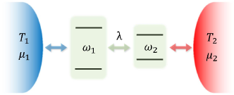
Figure 2: Two qubits with different frequencies weakly coupled with two environments. The two environments have different temperatures or chemical potentials. The inter-qubit coupling is characterized by $\lambda$.

We study a two-coupled two-level (qubit) system (with different transition frequencies) individually coupled to two bosonic or fermionic baths, respectively, with different temperatures or chemical potentials (see FIG. 2). The free Hamiltonian of the system (coupled two qubits) and the environments are given by

$$H_{S}=\omega_{1}|e_{1}\rangle\langle e_{1}|+\omega_{2}|e_{2}\rangle\langle e_{2}|+\frac{\lambda}{2}\left(\sigma_{1}^{+}\sigma_{2}^{-}+\sigma_{1}^{-}\sigma_{2}^{+}\right),$$ (17)

$$H_{R}=\sum_{k}\omega_{bk}b_{k}^{\dagger}b_{k}+\sum_{k}\omega_{ck}c_{k}^{\dagger}c_{k}$$ (18)

where $\omega_{1}$ and $\omega_{2}$ represent the energy splittings (transition frequencies) of the first and second qubit respectively; state $|e_{1}\rangle$ or $|e_{2}\rangle$ is the excitation in the first or second qubit; the ground state has energy 0; the third term in $H_{S}$ describes the coupling between the two qubits and $\lambda$ is the coupling strength between qubit 1 and qubit 2; operators $\sigma_{1}^{+}=|e_{1}\rangle\langle g_{1}|$ and $\sigma_{2}^{+}=|e_{2}\rangle\langle g_{2}|$ are the raising (creation) operators for the qubit one and the qubit two respectively; The bosonic bath gives the commutative relation $[b_{k},b_{k^{\prime}}^{\dagger}]=\delta_{kk^{\prime}}$, $[b_{k},b_{k^{\prime}}]=0$ and the fermionic bath gives the anti-commutative relation $\{b_{k},b_{k^{\prime}}^{\dagger}\}=\delta_{kk^{\prime}}$, $\{b_{k},b_{k^{\prime}}\}=0$; the two baths have the energy spectral $\omega_{bk}$ and $\omega_{ck}$ for the $k$-th mode ($b$ denotes the first bath coupled with qubit number 1 and $c$ denotes the second bath coupled with qubit number 2). The constant $\hbar=1$ is set to 1 for convenience.

The model having the Hamiltonian $H_{S}$ in (17) can be understood as two spatial separated atoms coupled through the dipole-dipole interaction Petrosyan and Kurizki (2002). Note that the effective Hamiltonian of the dipole-dipole interaction characterizes the resonant coupling of two identical atoms which have $\omega_{1}=\omega_{2}$ Craig and Thirunamachandran (1998). In the language of spin chain, Hamiltonian $H_{S}$ in (17) describes the Heisenberg XY model ($\sigma_{x}\sigma_{x}$ and $\sigma_{y}\sigma_{y}$ interactions) and the two spins are subjected to inhomogeneous magnetic field (different transition frequencies) Lieb et al. (1961); Wang (2001); Kamta and Starace (2002); Quiroga et al. (2007). If the two-level system is understood as a (spin-degenerate) quantum dot: $|g\rangle$ as the empty site and $|e\rangle$ as the occupied site, the coupling between the two qubits is essentially the non-interaction tunneling Lambert et al. (2007); Wang and Wang (2019). The onsite energies characterized by $\omega_{i}$ can be controlled by the electrochemical potentials Hayashi et al. (2003). Note that the Hamiltonian $H_{S}$ in (17) does not include the interdot Coulomb interaction of the two sites (as a toy model for double quantum dots).

Because of the dipole-dipole interaction, atomic basis is not the eigenstate. The system forms the dimer eigenstates (with the new eigenenergies) defined by:

$$\omega_{gg}=0, |1\rangle= |gg\rangle,$$

$$\omega_{1}^{\prime}=\bar{\omega}-\frac{1}{2}\sqrt{\Delta\omega^{2}+\lambda^{2}}, |2\rangle= \cos\frac{\theta}{2}|eg\rangle+\sin\frac{\theta}{2}|ge\rangle,$$

$$\omega_{2}^{\prime}=\bar{\omega}+\frac{1}{2}\sqrt{\Delta\omega^{2}+\lambda^{2}}, |3\rangle= -\sin\frac{\theta}{2}|eg\rangle+\cos\frac{\theta}{2}|ge\rangle,$$

$$\omega_{ee}=\omega_{1}+\omega_{2}, |4\rangle= |ee\rangle$$ (19)

We use short notations: $|eg\rangle=|e_{1}\rangle\otimes|g_{2}\rangle$. Here, $\bar{\omega}=(\omega_{1}+\omega_{2})/2$ is the mean energy splitting and $\Delta\omega=\omega_{1}-\omega_{2}$ is the degree of energy detuning. The interqubit interaction is relatively weak. We limit the coupling strength in the regime $\lambda<\sqrt{\omega_{1}\omega_{2}}$. The angle $\theta$ is defined by

$$\theta=\begin{cases}\arctan(\lambda/\Delta\omega),&\text{if~{}}\Delta\omega<0\\ \arctan(\lambda/\Delta\omega)-\pi,&\text{if~{}}\Delta\omega>0\end{cases}$$ (20)

The identical two qubits ($\omega_{1}=\omega_{2}=\omega$) gives $\theta=-\pi/2$. And the eigenstates $|2\rangle$ and $|3\rangle$ are Bell-type states (maximal entangled two-qubit states). The weak interqubit coupling $\lambda<\sqrt{\omega_{1}\omega_{2}}$ gives the ground state $|gg\rangle$. We have quantum phase transition Sachdev (2007) at $\lambda=\sqrt{\omega_{1}\omega_{2}}$: state $|2\rangle$ will be ground state if $\lambda>\sqrt{\omega_{1}\omega_{2}}$.

We can expand the lowering (annihilation) operators $\sigma_{l}^{-}$ (with $l=1,2$) and raising (creation) operators $\sigma_{l}^{+}$ into the basis of eigenstates $|j\rangle$ (with $j=1,2,3,4$):

$$\sigma_{1}^{-}=\eta_{1}+\xi_{1},\quad\quad\sigma_{2}^{-}=\eta_{2}+\xi_{2}$$ (21)

with the operators $\eta$ and $\xi$ defined in the energy basis

$$\eta_{1}= \cos\frac{\theta}{2}\left(|1\rangle\langle 2|+|3\rangle\langle 4|\right),$$ (22a)

$$\eta_{2}= \cos\frac{\theta}{2}\left(|1\rangle\langle 2|-|3\rangle\langle 4|\right),$$ (22b)

$$\xi_{1}= \sin\frac{\theta}{2}\left(|2\rangle\langle 4|-|1\rangle\langle 3|\right),$$ (22c)

$$\xi_{2}= \sin\frac{\theta}{2}\left(|2\rangle\langle 4|+|1\rangle\langle 3|\right)$$ (22d)

Similarly, the raising operators $\sigma_{l}^{+}$ can be reformulated with the operators $\eta^{\dagger}_{l}$ and $\xi^{\dagger}_{l}$ (with $l=1,2$).

We adopt the rotation wave approximation (neglecting oscillations with high frequency) to describe the interaction between the system and the environments:

$$H_{SR}=\sum_{k}g_{k}\left(\sigma^{-}_{1}b_{k}^{\dagger}+\sigma^{+}_{1}b_{k}\right)+\sum_{k}h_{k}\left(\sigma^{-}_{2}c_{k}^{\dagger}+\sigma^{+}_{2}c_{k}\right)$$ (23)

where $g_{k}$ and $h_{k}$ are the coupling strengths between the system and the environments. We can assume that $g_{k}$ and $h_{k}$ are both real numbers without losing generality. When the environments are bosonic (operators $b_{k}$ and $c_{k}$ follow the commutative relations), the model describes two atoms or two 1/2-spin system interacting with photonic or thermal baths. When the environments are fermionic (operators $b_{k}$ and $c_{k}$ follow the anti-commutative relations), the model describes double quantum dots coupled with two metal leads.

In the interaction picture, the Hamiltonian $H_{SR}$ (23) takes the form

$$H_{SR}(t)= \sum_{k}g_{k}\left(\eta_{1}e^{-i\omega^{\prime}_{1}t}+\xi_{1}e^{-i\omega^{\prime}_{2}t}\right)b_{k}^{\dagger}e^{i\omega_{bk}t}+\text{H.c.}$$

$$+ \sum_{k}h_{k}\left(\eta_{2}e^{-i\omega^{\prime}_{1}t}+\xi_{2}e^{-i\omega^{\prime}_{2}t}\right)c_{k}^{\dagger}e^{i\omega_{ck}t}+\text{H.c.}$$ (24)

where H.c. is short for Hermitian conjugate. The physical meaning of operators $\eta_{l}$ and $\xi_{l}$ (22a)-(22d) is clear: operators $\eta_{l}$ are lowering the energy $\omega_{1}^{\prime}$ and operators $\xi_{l}$ are lowering the energy $\omega^{\prime}_{2}$.

III.2 Quantum Master Equation

Based on the weak-coupling (between the system and environment) and Born-Markov approximations, the dynamics of system (in the interaction picture) is governed by the quantum master equation for the reduced density matrix (after tracing over the baths): Breuer and Petruccione (2002)

$$\frac{d\rho_{I}(t)}{dt}=-\int_{0}^{\infty}ds\text{Tr}_{R}\left[H_{SR}(t),\left[H_{SR}(t-s),\rho_{I}(t)\otimes\rho_{R}\right]\right]$$ (25)

where $\rho_{I}(t)=\exp\left(-iH_{S}t\right)\rho_{S}\exp\left(iH_{S}t\right)$ and $\rho_{R}$ is the density matrix of the two baths in their thermal equilibrium states. Here $i$ is the imaginary unit $i=\sqrt{-1}$. The above equation is called Bloch-Redfield equation Breuer and Petruccione (2002); Bloch (1957); Redfield (1957). For our model described by the interaction Hamiltonian $H_{SR}$ defined in (23), we have the Bloch-Redfield equation (back to Schrödinger’s picture):

$$\frac{d\rho_{S}}{dt}=i\left[\rho_{S},H_{S}\right]+\sum_{l=1}^{2}\mathcal{D}_{l}[\rho]$$ (26)

with the dissipators expressed as ($l=1,2$)

$$\mathcal{D}_{l}[\rho]= \alpha_{l}(\omega_{1}^{\prime})\left(\eta_{l}^{\dagger}\rho\eta_{l}+\eta_{l}^{\dagger}\rho\xi_{l}-\eta_{l}\eta_{l}^{\dagger}\rho-\xi_{l}\eta_{l}^{\dagger}\rho+\text{H.c.}\right)$$

$$+ \alpha_{l}(\omega_{2}^{\prime})\left(\xi_{l}^{\dagger}\rho\xi_{l}+\eta_{l}^{\dagger}\rho\xi_{l}-\xi_{l}\xi_{l}^{\dagger}\rho-\eta_{l}\xi_{l}^{\dagger}\rho+\text{H.c.}\right)$$

$$+ \beta_{l}(\omega_{1}^{\prime})\left(\eta_{l}\rho\eta_{l}^{\dagger}+\eta_{l}\rho\xi_{l}^{\dagger}-\eta_{l}^{\dagger}\eta_{l}\rho-\xi_{l}^{\dagger}\eta_{l}\rho+\text{H.c.}\right)$$

$$+ \beta_{l}(\omega_{2}^{\prime})\left(\xi_{l}\rho\xi_{l}^{\dagger}+\eta_{l}\rho\xi_{l}^{\dagger}-\xi_{l}^{\dagger}\xi_{l}\rho-\eta_{l}^{\dagger}\xi_{l}\rho+\text{H.c.}\right)$$ (27)

Here, the coefficients are

$$\alpha_{l}(\omega)=J_{l}(\omega)n_{l}(\omega),\quad\quad\beta_{l}(\omega)=J_{l}(\omega)(1\pm n_{l}(\omega))$$ (28)

with the coupling spectrum of the two baths defined as:

$$J_{1}(\omega)=\pi\sum_{k}g_{k}^{2}\delta(\omega-\omega_{bk}),\quad J_{2}(\omega)=\pi\sum_{k}h_{k}^{2}\delta(\omega-\omega_{ck})$$ (29)

Here the plus sign in $\beta_{l}(\omega)$ is for the case of the bosonic bath and the minus sign is for the fermionic bath. Variable $n_{l}(\omega)$ is the mean occupation number of particles with the energy $\omega$ at temperature $T_{l}$ and chemical potential $\mu_{l}$ for the $l$-th bath, namely

$$n_{l}(\omega)=\frac{1}{\exp\left((\omega-\mu_{l})/T_{l}\right)\mp 1}$$ (30)

The minus sign is for bosonic bath (Bose-Einstein distribution) and plus sign is for fermionic bath (Fermi-Dirac distribution). Boltzmann constant is set to be 1. Photons or phonons have negligible self-interactions. We set $\mu_{1}=\mu_{2}=0$ both for the equilibrium ($T_{1}=T_{2}=T$) and nonequilibrium ($T_{1}\neq T_{2}$) bosonic baths. And we consider the temperature equilibrium ($T_{1}=T_{2}=T$) for fermionic baths both for equilibrium chemical potential ($\mu_{1}=\mu_{2}=\mu$) and nonequilibrium chemical potential ($\mu_{1}\neq\mu_{2}$) cases, especially in the low-temperature regime.

Operators $\eta_{l}$ defined in (22a) and (22b) and $\xi_{l}$ defined in (22c) and (22d) characterize the transitions with different frequencies ($\eta_{l}$ is for $\omega_{1}^{\prime}$ and $\xi_{l}$ is for $\omega_{2}^{\prime}$). In the interaction picture, cross terms in the dissipators in (III.2), such as $\eta_{l}^{\dagger}\rho\xi_{l}$, are usually considered as oscillating processes and therefore often neglected under fast oscillations (secular approximation). After secular approximation, the Bloch-Redfield equation becomes the Lindblad form. Since the cross terms couple the population and coherent space of the density matrix, dropping the crossing terms gives zero steady state coherence (in the eigenstate representation) (see Li et al. (2015); Wang et al. (2018, 2019)). Coherence is crucial for the violations of LGIs. Therefore, we keep the cross terms in our study and apply the master equation without the secular approximation, or the Bloch-Redfield equation for time evolution of the system.

III.3 Steady State Solutions

The steady-state solution of the Bloch-Redfield equation in a similar setting (for the study of a different problem) had been obtained in Wang et al. (2019). Here, we follow the similar procedure. We can reformulate the Bloch-Redfield equation with the form (26) in the Liouville space, where the system density matrix takes the vector form

$$|\rho_{S}\rangle=\left(\rho_{11},\rho_{22},\rho_{33},\rho_{44},\rho_{23},\rho_{32}\right)^{T}$$ (31)

with $T$ as the matrix transpose. Other coherence terms (such as $\rho_{14}$ and $\rho_{41}$) are decoupled with the population terms and therefore can be dropped in the steady-state solution. The Bloch-Redfield equation (26) has the matrix form:

$$\frac{d}{dt}|\rho_{S}\rangle=\mathcal{M}|\rho_{S}\rangle$$ (32)

The expressions of the matrix elements $\mathcal{M}$ are given in Appendix A.

The reduced density matrix of system can be grouped into two parts: $|\rho_{S}\rangle=\left(\rho_{p},\rho_{c}\right)^{T}$ with population terms $\rho_{p}$ (diagonal terms) and coherence terms $\rho_{c}$ (off-diagonal terms). Under the same arguments, the dynamic matrix $\mathcal{M}$ has the block forms:

$$\mathcal{M}=\left(\begin{array}[]{cc}\mathcal{M}_{pp}&\mathcal{M}_{pc}\\ \mathcal{M}_{cp}&\mathcal{M}_{cc}\end{array}\right)$$ (33)

The steady state is given by

$$\mathcal{M}|\rho^{\text{ss}}_{S}\rangle=0$$ (34)

The coherence terms can be substituted by

$$\rho_{c}=-\mathcal{M}_{cc}^{-1}\mathcal{M}_{cp}\rho_{p}$$ (35)

with invertible block matrix $\mathcal{M}_{cc}$. Then, we define the steady-state population matrix $\mathcal{A}$ as

$$\mathcal{A}=\mathcal{M}_{pp}-\mathcal{M}_{pc}\mathcal{M}_{cc}^{-1}\mathcal{M}_{cp}$$ (36)

which satisfies

$$\mathcal{A}|\rho^{\text{ss}}_{p}\rangle=0$$ (37)

Note that the overall constant in $\mathcal{A}$ gives the same steady state solution. The matrix elements of the steady-state population matrix $\mathcal{A}$, both for the bosonic and fermionic baths, are presented in Appendix B.

In the following, we consider the symmetric constant coupling spectrum:

$$J_{1}(\omega)=J_{2}(\omega)=J$$ (38)

To simplify the steady-state expressions $\rho^{\text{ss}}_{S}$, we introduce the following notations:

$$\tilde{n}_{1}(\theta,\omega_{1}^{\prime})=\cos^{2}\frac{\theta}{2}n_{1}(\omega^{\prime}_{1})+\sin^{2}\frac{\theta}{2}n_{2}(\omega^{\prime}_{1}),$$ (39a)

$$\tilde{n}_{2}(\theta,\omega_{2}^{\prime})=\sin^{2}\frac{\theta}{2}n_{1}(\omega^{\prime}_{2})+\cos^{2}\frac{\theta}{2}n_{2}(\omega^{\prime}_{2}),$$ (39b)

$$\Delta n_{1}(\theta,\omega_{1}^{\prime})=\frac{1}{2}\sin\theta\left(n_{2}(\omega^{\prime}_{1})-n_{1}(\omega^{\prime}_{1})\right),$$ (39c)

$$\Delta n_{2}(\theta,\omega_{2}^{\prime})=\frac{1}{2}\sin\theta\left(n_{2}(\omega^{\prime}_{2})-n_{1}(\omega^{\prime}_{2})\right)$$ (39d)

To avoid tedious notations, we set

$$\tilde{n}_{l}\equiv\tilde{n}_{l}(\theta,\omega_{l}^{\prime}),\quad\Delta n_{l}\equiv\Delta n_{l}(\theta,\omega_{l}^{\prime})$$ (40)

with $l=1,2$. Here $\tilde{n}_{l}$ can be viewed as the mean particle occupation number weighted by the mixing angle $\theta$ in the two baths with the same energy $\omega_{l}^{\prime}$. And $\Delta n_{l}$ describes the difference in occupation number and therefore the degree of the nonequilibriumness which vanishes at the equilibrium case $T_{1}=T_{2}$ and $\mu_{1}=\mu_{2}$.

III.3.1 Steady state solution for bosonic bath

Directly solving the steady-state equation (37) for bosonic baths (the matrix $\mathcal{A}^{\text{b}}$ for bosonic baths has the elements in (127)-(142)) gives the steady solution Wang et al. (2019):

$$\rho^{\text{b}}_{11}= \frac{1}{\mathcal{N}^{\text{b}}}\left((1+\tilde{n}_{1})(1+\tilde{n}_{2})-\frac{\kappa^{\text{b}}s_{1}s_{2}}{4(1+\tilde{n}_{1}+\tilde{n}_{2})}\right),$$ (41a)

$$\rho^{\text{b}}_{22}= \frac{1}{\mathcal{N}^{\text{b}}}\left(\tilde{n}_{1}(1+\tilde{n}_{2})+\frac{\kappa^{\text{b}}s_{2}s_{3}}{4(1+\tilde{n}_{1}+\tilde{n}_{2})}\right),$$ (41b)

$$\rho^{\text{b}}_{33}= \frac{1}{\mathcal{N}^{\text{b}}}\left(\tilde{n}_{2}(1+\tilde{n}_{1})+\frac{\kappa^{\text{b}}s_{1}s_{4}}{4(1+\tilde{n}_{1}+\tilde{n}_{2})}\right),$$ (41c)

$$\rho^{\text{b}}_{44}= \frac{1}{\mathcal{N}^{\text{b}}}\left(\tilde{n}_{1}\tilde{n}_{2}-\frac{\kappa^{\text{b}}s_{3}s_{4}}{4(1+\tilde{n}_{1}+\tilde{n}_{2})}\right)$$ (41d)

Here, $\kappa^{\text{b}}$ is defined as

$$\kappa^{\text{b}}=\frac{\tilde{n}_{1}+\tilde{n}_{2}+1}{(\tilde{n}_{1}+\tilde{n}_{2}+1)^{2}+(\Omega/2J)^{2}}$$ (42)

with the transition frequency given as

$$\Omega=\omega_{2}^{\prime}-\omega_{1}^{\prime}=\sqrt{\Delta\omega^{2}+\lambda^{2}}$$ (43)

Note that $\kappa^{\text{b}}$ is also defined in the population matrix $\mathcal{A}^{\text{b}}$ [see (126]. The other parameters are

$$s_{1}=\Delta n_{2}-\Delta n_{1}(3+2\tilde{n}_{1}+2\tilde{n}_{2}),$$ (44a)

$$s_{2}=\Delta n_{1}-\Delta n_{2}(3+2\tilde{n}_{1}+2\tilde{n}_{2}),$$ (44b)

$$s_{3}=\Delta n_{2}+\Delta n_{1}(1+2\tilde{n}_{1}+2\tilde{n}_{2}),$$ (44c)

$$s_{4}=\Delta n_{1}+\Delta n_{2}(1+2\tilde{n}_{1}+2\tilde{n}_{2}),$$ (44d)

The normalization $\mathcal{N}^{\text{b}}$ is

$$\mathcal{N}^{\text{b}}=(1+2\tilde{n}_{1})(1+2\tilde{n}_{2})-4\kappa_{b}\Delta n_{1}\Delta n_{2}(1+\tilde{n}_{1}+\tilde{n}_{2})$$ (45)

The superscript “b” stands for the bosonic reservoir setup. We omit the superscript “ss” for the steady-state notation.

The steady state coherence is given by (35). We have

$$\rho^{\text{b}}_{23}={\rho^{\text{b}}_{32}}^{*}=\frac{1}{\mathcal{N}_{b}}\left(\frac{\Delta n_{1}(1+2\tilde{n}_{2})+\Delta n_{2}(1+2\tilde{n}_{1})}{2(1+\tilde{n}_{1}+\tilde{n}_{2})-i\Omega/J}\right)$$ (46)

which vanishes if $\Delta n_{1}=\Delta n_{2}=0$, namely at the equilibrium case, off-diagonal terms of the reduced density matrix at steady state in the energy basis are always zero. The asterisk represents the complex conjugate.

Parameters $s_{j}$ with $j=1,2,3,4$ defined in (44a)-(44d) solely characterize the nonequilibrium effects, since they all vanish at equilibrium cases. We can view the second terms in (41a)-(41d) as the nonequilibrium corrections which are proportional to the square of coupling strength $J^{2}$ (since $\kappa^{\text{b}}$ (42) is proportional to $J^{2}$). Although $J^{2}$ is negligible (weak coupling assumption), the nonequilibrium correction terms such as $J^{2}\Delta\tilde{n}^{2}_{l}$ are not bounded (only in the case of bosonic baths). The first term of the steady-state population in (41a)-(41d) can only reveal part of the nonequilibrium effects (the mean properties of the two baths) if we have intermediate temperature difference. In other words, the Lindblad can be used to characterize some nonequilibrium results Sinaysky et al. (2008); Wu and Segal (2011); Castillo et al. (2013); Wang and Wang (2019). However, we will see later that the LGI function and MLGI function obtained by the Bloch-Redfield equation can have significant deviations from those characterized by the Lindblad, due to the dynamic differences.

Equilibrium case ($T_{1}=T_{2}=T$) gives vanishing $\Delta n_{i}$ with $i=1,2$ (defined in (39c) and (39d)). Therefore, we do not have coherence $\rho_{23}^{\text{b}}$ in the energy basis. We have the equilibrium steady state:

$$\rho^{\text{b,e}}_{11}= \frac{1}{\mathcal{N}^{\text{b,e}}}(1+\tilde{n}_{1})(1+\tilde{n}_{2}), \rho^{\text{b,e}}_{22}= \frac{1}{\mathcal{N}^{\text{b,e}}}\tilde{n}_{1}(1+\tilde{n}_{2}),$$

$$\rho^{\text{b,e}}_{33}= \frac{1}{\mathcal{N}^{\text{b,e}}}\tilde{n}_{2}(1+\tilde{n}_{1}), \rho^{\text{b,e}}_{44}= \frac{1}{\mathcal{N}^{\text{b,e}}}\tilde{n}_{1}\tilde{n}_{2}$$ (47)

with the normalization

$$\mathcal{N}^{\text{b,e}}=(1+2\tilde{n}_{1})(1+2\tilde{n}_{2})$$ (48)

The superscript “e” reminds the equilibrium situation. The equilibrium steady state satisfies the canonical ensemble distribution. At low temperatures, the system stays at the ground state with high probability:

$$\lim_{T\rightarrow 0}\rho^{\text{b,e}}_{11}=1$$ (49)

At high temperatures, we have the equally mixed state:

$$\lim_{T\rightarrow\infty}\rho^{\text{b,e}}_{jj}=\frac{1}{4}$$ (50)

with $j=1,2,3,4$.

III.3.2 Steady state solution for fermionic bath

When the system is coupled with two fermionic baths (double quantum dots as the system), we have the steady-state population matrix $\mathcal{A}^{\text{f}}$ with matrix elements given in (143)-(156). We can solve the reduced steady-state density matrix Wang et al. (2019):

$$\rho^{\text{f}}_{11}= (1-\tilde{n}_{1})(1-\tilde{n}_{2})-\frac{\kappa^{\text{f}}}{4}\left(\Delta n_{1}+\Delta n_{2}\right)^{2},$$ (51a)

$$\rho^{\text{f}}_{22}= \tilde{n}_{1}(1-\tilde{n}_{2})+\frac{\kappa^{\text{f}}}{4}\left(\Delta n_{1}+\Delta n_{2}\right)^{2},$$ (51b)

$$\rho^{\text{f}}_{33}= \tilde{n}_{2}(1-\tilde{n}_{1})+\frac{\kappa^{\text{f}}}{4}\left(\Delta n_{1}+\Delta n_{2}\right)^{2},$$ (51c)

$$\rho^{\text{f}}_{44}= \tilde{n}_{1}\tilde{n}_{2}-\frac{\kappa^{\text{f}}}{4}\left(\Delta n_{1}+\Delta n_{2}\right)^{2}$$ (51d)

with $\kappa^{\text{f}}$ defined as

$$\kappa^{\text{f}}=\frac{1}{1+(\Omega/2J)^{2}}$$ (52)

The superscript “f” means the fermionic bath setup. The corresponding coherence terms of the reduced density matrix are

$$\rho^{\text{f}}_{23}={\rho^{\text{f}}_{32}}^{*}=\frac{\Delta n_{1}+\Delta n_{2}}{2-i\Omega/J}$$ (53)

which is zero if $\Delta n_{1}=\Delta n_{2}=0$. Nonequilibrium corrections (second terms in (51a)-(51d)) are proportional to $J^{2}\Delta n^{2}_{l}$. Unlike the bosonic environments, the particle occupation number difference $|\Delta n_{l}|<1/2$ is bounded in the fermionic case. Therefore, for $J\ll\Omega$, the Lindblad form can give reasonable description for effects of the nonequilibrium fermionic environments.

The equilibrium steady state ($T_{1}=T_{2}=T$ and $\mu_{1}=\mu_{2}=\mu$) is the special case of (51a)-(51d) with $\Delta n_{1}=\Delta n_{2}=0$:

$$\rho^{\text{f,e}}_{11}= (1-\tilde{n}_{1})(1-\tilde{n}_{2}), \rho^{\text{f,e}}_{22}= \tilde{n}_{1}(1-\tilde{n}_{2})$$

$$\rho^{\text{f,e}}_{33}= \tilde{n}_{2}(1-\tilde{n}_{1}), \rho^{\text{f,e}}_{44}= \tilde{n}_{1}\tilde{n}_{2}$$ (54)

which satisfies the grand canonical ensemble distribution ($\mu\neq 0$). At low chemical potentials, we reach

$$\lim_{\mu\rightarrow 0}\rho^{\text{f,e}}_{11}=1$$ (55)

The double dots are both empty. When we have high chemical potentials (with low temperatures), we reach

$$\lim_{\mu\rightarrow\infty}\rho^{\text{f,e}}_{44}=1$$ (56)

We have two occupied sites.

IV Leggett-Garg inequalities violations in equilibrium cases

The two- and three-time LGIs defined in (13) and (9) impose constraints on the two-time and one-time probability distributions if they are obtained from the marginals of the joint three-time probabilities. In this section, we explore the LGIs for our two-qubit system with the equilibrium environments (two bosonic baths have the same temperatures or two fermionic baths have the same temperatures and chemical potentials). First we numerically show that not all LGIs are violated. We define the maximum of LGIs (MLGI) function. Note that the dynamics of the system is described by the Bloch-Redfield equation (26). It is difficult to give the closed expression of the time-evolution operator given any time $t$. In the following, we calculate the time-evolution operator in a perturbative way, namely the time-evolution operator in the zeroth and the first order of the coupling $J$ defined in (29). Such perturbation is valid if the system and bath are weakly coupled and the equilibrium temperature is relatively low. The weakly coupling condition is also the assumption for deriving the Bloch-Redfield equation (26). We study the MLGI function both analytically and numerically.

IV.1 Maximum of the Leggett-Garg Inequalities

The time-evolution operator for the reduced density matrix (the two qubit system) is generated by the superoperator $\mathcal{W}$, which is given by the Bloch-Redfield equation in Eq. (26). The superoperator $\mathcal{W}$ has two parts: the coherent evolution $\mathcal{W}_{0}$ and the dissipator $\mathcal{W}_{d}$. The coherent evolution is the unitary part defined by the von Neumann equation:

$$\mathcal{W}_{0}\rho_{S}=i[\rho_{S},H_{S}]$$ (57)

where $H_{S}$ is the system Hamiltonian defined in (17). The dissipator originates from the interaction between the system and the environments, defined in (III.2). Then the quantum correlation function $C_{\text{q}}(t)$ in (II.1) is calculated from

$$C_{\text{q}}(t)=\mathrm{Re}\mathrm{Tr}\left(Qe^{\mathcal{W}t}Q\rho^{\text{ss}}\right)$$ (58)

Note that to exclude the invasiveness on the macrorealism tests, the correlation function $C_{\text{q}}(t)$ is measured according to the INM protocol described in Sec. II.4.

The states $|g\rangle$ and $|e\rangle$ represent the local realism of the system. Although we can optimize the choice of local observables in order to maximize the violations of the LGIs Emary (2013), we fix the observables to compare the violation of the LGIs with different environmental contexts. We choose the standard single-qubit dichotomic observable

$$Q=\sigma_{z,1}=(|g\rangle\langle g|-|e\rangle\langle e|)\otimes 1\!\!1_{2}$$ (59)

to testify the LGIs. In the energy basis (III.1), the observable $Q$ has the matrix form

$$Q=\left(\begin{array}[]{cccc}1&0&0&0\\ 0&-\cos\theta&\sin\theta&0\\ 0&\sin\theta&\cos\theta&0\\ 0&0&0&-1\end{array}\right)$$ (60)

with $\theta$ defined in (20).

First, we give an numerical results on the LGI functions $\mathcal{I}_{\pm}(t,\rho^{\text{ss}})$ and $\mathcal{I}_{2}(t,\rho^{\text{ss}})$ defined in (10) and (14) respectively, see FIG. 3. We consider the case that two-qubit system is coupled with the equilibrium environments, where the two baths have the same temperatures and the same chemical potentials. Since the bosonic and fermionic baths have different statistics, they give different steady states (and different dynamics), see Eq. (III.3.1) and (III.3.2), we draw the LGI functions for the bosonic and fermionic environments separately in FIG. 3. Clearly we can see that all the three LGI functions are damped due to the non-unitary evolution of the system. However, only the LGI function $\mathcal{I}_{+}(t,\rho^{\text{ss}})$ exceeds the classical limit either in the bosonic case or the fermionic case. We will give the analytical argument that only the LGI function $\mathcal{I}_{+}(t,\rho^{\text{ss}})$ is violated irrespective to the initial steady state in Sec. IV.2.

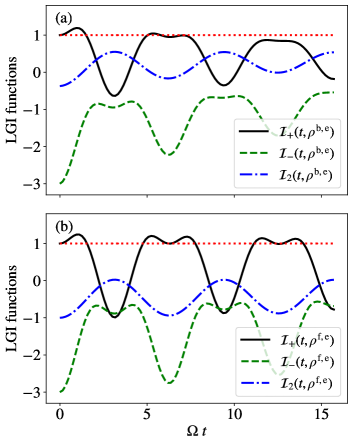
Figure 3: LGI functions $\mathcal{I}_{\pm}(t,\rho^{\text{ss}})$ in (10) and $\mathcal{I}_{2}(t,\rho^{\text{ss}})$ in (14) for the two-qubit system coupled with equilibrium environments. The oscillating frequency $\Omega$ is defined in Eq. (43). The parameters are set as $\lambda=\bar{\omega}$, $\theta=-\pi/2$ and $J=0.005\bar{\omega}$. (a) The two-qubit system is coupled with two bosonic baths with the same temperature $T=1.5\bar{\omega}$. (b) The two-qubit system is coupled with two fermionic baths with the same temperature $T=1.5\bar{\omega}$ and the same chemical potentials $\mu=\bar{\omega}$. The above red line suggests the violations of LGIs (beyond the classical description).

To characterize the violations of the LGIs, we define the MLGI function by

$$\mathcal{I}_{\text{max}}(\rho^{\text{ss}})=\max_{t\geq 0}\left\{\mathcal{I}_{\pm}(t,\rho^{\text{ss}}),\frac{1}{2}\mathcal{I}_{2}(t,\rho^{\text{ss}})\right\}-1$$ (61)

The overall $1/2$ constant before the LGI function $\mathcal{I}_{2}(t,\rho^{\text{ss}})$ is for normalizing to the same maximal value with the LGI functions $I_{\pm}(t,\rho^{\text{ss}})$. The minimal value of $\mathcal{I}_{\text{max}}(\rho^{\text{ss}})$ is 0 since we have

$$\mathcal{I}_{+}(0,\rho^{\text{ss}})=1$$ (62)

Violations of the LGIs in (10) and (14) give $\mathcal{I}_{\text{max}}(\rho^{\text{ss}})>0$, which suggests that the quantum evolution (of the system) is beyond the classical descriptions (no joint probability distribution for observables at different times) Emary et al. (2013). Unitary evolution (full quantum description) of quantum states gives the maximal value of $\mathcal{I}_{\text{max}}(\rho^{\text{ss}})$. We have the range:

$$0\leq\mathcal{I}_{\text{max}}(\rho^{\text{ss}})\leq\frac{1}{2}$$ (63)

MLGI function is a natural quantity characterizing the maximal degree of LGIs violations. MLGI function is also the witness of the quantum evolution, which is beyond the classical probability evolution.

IV.2 Leggett-Garg Inequalities in the Zeroth Order of Coupling

The analytical form of the time-evolution operator $e^{\mathcal{W}t}$ given by the Bloch-Redfield equation in Eq. (26) is complicated. We consider the perturbation method. The time-evolution operator to the zeroth order of the coupling is the superoperator with the coherent evolution only. In zeroth order of the coupling $J$, the correlation function $C_{\text{q}}(t)$ defined in (II.1) is obtained from the coherent evolution $\mathcal{W}_{0}$. We have

$$C^{(0)}_{\text{q}}(t,\rho)=1-(1-\cos(\Omega t))\sin^{2}\theta(\rho_{22}+\rho_{33})$$ (64)

The frequency $\Omega$ is defined in (43). The zeroth order correlation function $C^{(0)}_{\text{q}}(t)$ oscillates with the period $\Omega/2\pi$. We have the perfect oscillation (without decay) because the coupling to the environments is turned off. If we turn off the interqubit coupling, i.e., $\lambda=0$, which means the two-qubit systems are decoupled, we have

$$C^{(0)}_{\text{q}}(t,\rho(\lambda=0))=1$$ (65)

We have the perfect correlation because the observable $Q$ defined in Eq. (59) commutes with the Hamiltonian $H_{S}$ when $\lambda=0$.

Let us firstly look up the zeroth order of two-time LGI function $\mathcal{I}_{2}(t,\rho^{\text{ss}})$ defined in Eq. (14), which has the form

$$\mathcal{I}^{(0)}_{2}(t,\rho^{\text{ss}})=2(\rho^{\text{ss}}_{11}-\rho^{\text{ss}}_{44})+2\cos\theta(\rho^{\text{ss}}_{33}-\rho^{\text{ss}}_{22})\\ +4\sin\theta\mathrm{Re}\rho^{\text{ss}}_{23}+(1-\cos(\Omega t))\sin^{2}\theta(\rho^{\text{ss}}_{22}+\rho^{\text{ss}}_{33})-1$$ (66)

Obviously, the maximum of $\mathcal{I}^{(0)}_{2}(t,\rho^{\text{ss}})$ is at $t=(2k+1)\pi/\Omega$ with $k=0,1,\cdots$. If we have the equilibrium environments, the steady state coherence in the energy basis vanishes, i.e., $\rho^{\text{ss}}_{23}=0$. One can verify that the steady state $\rho^{\text{ss}}$ either in the bosonic case or in the fermionic case has the relation $\rho^{\text{ss}}_{33}<\rho^{\text{ss}}_{22}$. Therefore, the detuning angle $\theta=-\pi/2$ gives the maximum of $\mathcal{I}^{(0)}_{2}(t,\rho^{\text{ss}})$ when $t=(2k+1)\pi/\Omega$. Based on the above optimal choices of the parameters, we have

$$\mathcal{I}^{(0)}_{2}(t=\pi/\Omega,\rho^{\text{ss}}(\theta=-\pi/2))\\ =2(\rho^{\text{ss}}_{11}-\rho^{\text{ss}}_{44})+2(\rho^{\text{ss}}_{22}+\rho^{\text{ss}}_{33})-1$$ (67)

It is easy to see that the two-time LGI function in the zeroth order $\mathcal{I}^{(0)}_{2}(t,\rho^{\text{ss}})$ does not violate the classical bound:

$$\mathcal{I}^{(0)}_{2}(t,\rho^{\text{ss}})\leq 1$$ (68)

Single qubit with Rabi oscillation can violate the two-time LGIs dependent on the initial state Halliwell (2016); Majidy et al. (2019). Here the two-time LGIs are not violated (two qubits coupled with the equilibrium environments) because of the nature of the steady state and the specific dynamics of the system.

Given by the zeroth order correlation function $C^{(0)}_{\text{q}}(t,\rho)$ in Eq. (64), the three-time LGI functions $\mathcal{I}_{\pm}(t,\rho^{\text{ss}})$ defined in Eq. (10) have the forms

$$\mathcal{I}_{+}^{(0)}(t,\rho^{\text{ss}})\\ =1+\left(2\cos(\Omega t)-\cos(2\Omega t)-1\right)\sin^{2}\theta(\rho^{\text{ss}}_{22}+\rho^{\text{ss}}_{33})$$ (69)

$$\mathcal{I}_{-}^{(0)}(t,\rho^{\text{ss}})\\ =-3+(3-2\cos(\Omega t)-\cos(2\Omega t))\sin^{2}\theta(\rho^{\text{ss}}_{22}+\rho^{\text{ss}}_{33})$$ (70)

It is easy to find that the zeroth order of three time LGI functions $\mathcal{I}_{+}^{(0)}(t,\rho^{\text{ss}})$ and $\mathcal{I}_{-}^{(0)}(t,\rho^{\text{ss}})$ have the first maximums at $t=\pi/(3\Omega)$ and $t=2\pi/(3\Omega)$ respectively. And we have

$$\mathcal{I}_{+}^{(0)}(\pi/(3\Omega),\rho^{\text{ss}})=\frac{1}{2}\sin^{2}\theta(\rho^{\text{ss}}_{22}+\rho^{\text{ss}}_{33})+1$$ (71)

$$\mathcal{I}_{-}^{(0)}(2\pi/(3\Omega),\rho^{\text{ss}})=\frac{9}{2}\sin^{2}\theta(\rho^{\text{ss}}_{22}+\rho^{\text{ss}}_{33})-4$$ (72)

Obviously we have

$$\mathcal{I}_{+}^{(0)}(\pi/(3\Omega),\rho^{\text{ss}})\geq\mathcal{I}_{-}^{(0)}(2\pi/(3\Omega),\rho^{\text{ss}})$$ (73)

Only at $\theta=-\pi/2$ and $\rho^{\text{ss}}_{22}+\rho^{\text{ss}}_{33}=1$ we have the equal sign. The classical description of the LGI functions defined in (9) is bounded by 1. We have $\mathcal{I}_{+}^{(0)}(t,\rho^{\text{ss}})>1$ during the time $0<t<\pi/(2\Omega)$ and $(3/2+2k)\pi/\Omega<t<(5/2+2k)\pi/\Omega$ with $k=0,1,\cdots$, as long as we have (nonzero) steady state population $(\rho_{22}+\rho_{33})$ and nonzero inter-qubit coupling $\lambda\neq 0$.

According to the maximum of the three-time LGI functions $\mathcal{I}_{\pm}^{(0)}(t,\rho^{\text{ss}})$ in Eqs. (71) and (72), we have the zeroth order of the MLGI function defined in (61):

$$\mathcal{I}_{\text{max}}^{(0)}(\rho^{\text{ss}})=\frac{1}{2}\sin^{2}\theta(\rho^{\text{ss}}_{22}+\rho^{\text{ss}}_{33})$$ (74)

Note that only the populations $\rho_{22}$ and $\rho_{33}$ contribute to the violation of LGIs, because states $|1\rangle$ and $|4\rangle$ defined in (III.1) are product states and their evolution admits classical descriptions (no off-diagonal terms). Also when $\lambda=0$ (the two-qubit systems are decoupled), eigenstates are all product states and the time-evolution operator for the local states is diagonalized (classical probabilistic descriptions). When we have two identical qubits ($\omega_{1}=\omega_{2}$), if the population for states $|2\rangle$ and $|3\rangle$ is maximal, i.e., $\rho^{\text{ss}}_{22}+\rho^{\text{ss}}_{33}=1$, the violation of LGI is saturated Emary et al. (2013). Notice that the symmetric qubits have eigenstates $|2\rangle$ and $|3\rangle$ as maximal entangled two qubit states (Bell-type states). We can see that the coherent evolution of the spatial maximal entangled states also has the maximal violation of LGIs. Then it is reasonable to view the maximum of the LGI functions defined in Eq. (61) as a quantitative measure for quantum evolution.

The zeroth order of LGI functions $\mathcal{I}_{\pm}^{(0)}(t,\rho^{\text{ss}})$ in Eqs. (71) and (72) oscillate without decay, which implies the information of the system is preserved (the LGI violations can occur at any long time interval between the two measurements). See FIG. 4 for the comparison between the zeroth order, the first order and the numerical LGI function $\mathcal{I}_{+}(t,\rho^{\text{ss}})$. The physical meaning of the zeroth order of LGI functions $\mathcal{I}_{2}^{(0)}(t,\rho^{\text{ss}})$ and $\mathcal{I}_{\pm}^{(0)}(t,\rho^{\text{ss}})$ is that the steady state (coupled with the environments) evolves coherently (decoupled from the environments) after the first measurement. The zeroth order LGI functions have the same form both in equilibrium and nonequilibrium cases (and the same for bosonic and fermionic baths), being different only in the steady state $\rho^{\text{ss}}$.

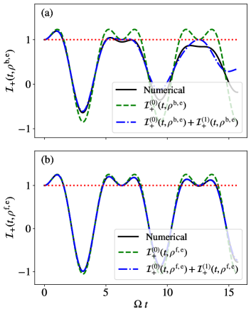
Figure 4: LGI function $\mathcal{I}_{+}(t,\rho^{\text{ss}})$ defined in (10) for the two-qubit system coupled with two (a) bosonic or (b) fermionic baths. The oscillating frequency $\Omega$ is defined in Eq. (43). Parameters are set as $\lambda=\bar{\omega}$, $\theta=-\pi/2$ and $J=0.005\bar{\omega}$. The solid line is the numerical results based on the Bloch-Redfield equation (26); the dashed line is the zeroth order $J$ of the LGI function $\mathcal{I}_{+}^{(0)}(t,\rho^{\text{ss}})$ in (69); the dotted-dashed line is up to the first order $J$ of the LGI function: $\mathcal{I}_{+}^{(0)}(t,\rho^{\text{ss}})+\mathcal{I}_{+}^{(1)}(t,\rho^{\text{ss}})$; analytical expression of $\mathcal{I}_{+}^{(1)}(t,\rho^{\text{b,e}})$ and $\mathcal{I}_{+}^{(1)}(t,\rho^{\text{f,e}})$ can be found in (83) and (89) respectively. Above the red line suggests the violation of LGIs (beyond the classical description). (a) Two bosonic baths have the same temperature $T=1.5\bar{\omega}$. (b). Two fermionic baths have the same chemical potentials $\mu=\bar{\omega}$ and temperatures $T=1.5\bar{\omega}$.

IV.3 Leggett-Garg Inequalities in the First Order Coupling

The superoperator $\mathcal{W}$ characterizing the time evolution of the system has the matrix form $\mathcal{M}$ (Liouville space), see (32). Then we have the time evolution:

$$|\rho_{S}(t)\rangle=e^{\mathcal{M}t}|\rho_{S}\rangle$$ (75)

Note that the evolution operator $e^{\mathcal{M}t}$ is defined in the energy basis. The analytical form of $e^{\mathcal{M}t}$ is complicated, even when the matrix $\mathcal{M}$ can be diagonalized. Note that the real part of $\mathcal{M}$ is related to the overall coupling constant $J$ and the imaginary part of $\mathcal{M}$ is related to the coherent oscillation only, namely we have

$$\mathcal{M}=\mathcal{M}_{0}+\mathcal{M}_{J}$$ (76)

with

$$\mathcal{M}_{J}=\mathrm{Re}\mathcal{M},\quad\mathcal{M}_{0}=i\mathrm{Im}\mathcal{M},$$ (77)

see the matrix elements of $\mathcal{M}$ in (A)-(A).

We can apply the Zassenhaus formula Kimura (2017) in the first order of the coupling constant $J$:

$$e^{\mathcal{M}t}=\left(1\!\!1+\sum_{n=1}^{\infty}\frac{t^{n}}{n!}\mathcal{L}_{\mathcal{M}_{0}}^{n-1}\mathcal{M}_{J}+\mathcal{O}(\mathcal{M}^{2}_{J})\right)e^{\mathcal{M}_{0}t}$$ (78)

where $\mathcal{L}$ is the commutator operator

$$\mathcal{L}_{\mathcal{M}_{0}}\mathcal{M}_{J}=[\mathcal{M}_{0},\mathcal{M}_{J}]$$ (79)

Evolution $\exp(\mathcal{M}_{0}t)$ is the coherent part discussed before. The above expansion is based on the small coupling $J$. More specifically, the matrix elements of $\mathcal{M}_{J}t$ should be much less than 1, formally

$$tJn_{l}(\omega^{\prime}_{1,2})\ll 1$$ (80)

It suggests that we have good agreements for the first-order LGI functions when $t$ is small, for example see FIG. 4. The approximation condition in Eq. (80) requires the low temperature: $T<\omega^{\prime}_{1,2}$ for bosonic reservoirs. Since the mean particle occupation number $n_{l}(\omega^{\prime}_{1,2})$ is bounded in fermionic baths due to the exclusion principle, we have the approximation condition $t\ll 1/J$. The bounded mean particle occupation number in fermionic cases also suggests we have better approximation in the first order LGI function, see FIG. 4. The systems are supposed to be “classical” and all LGIs are preserved when the environments are at high temperatures. We will numerically check that the LGIs are not violated in the high temperature regime.

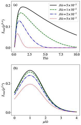
Figure 5: MLGI function $\mathcal{I}_{\text{max}}(\rho^{\text{b,e}})$ defined in (61) in terms of system-bath coupling $J$ and (a) equilibrium temperature $T=T_{1}=T_{2}$ for bosonic bath and (b) equilibrium chemical potential $\mu=\mu_{1}=\mu_{2}$ for fermionic bath with temperature $T=0.5\bar{\omega}$. Parameters are set as $\lambda=\bar{\omega}$ and $\theta=-\pi/2$.

IV.3.1 Equilibrium bosonic Bath

The equilibrium steady state does not have the coherence terms in the energy basis, i.e., the population space and coherence space are decoupled in the Bloch-Redfield equation, see (26). However, the coherence in the localized state representation always survives if we have non-vanishing inter-qubit coupling $\lambda$. Matrix elements of $\mathcal{M}$ in (32) is block diagonalized in the energy basis. Moreover, we can check that the real (dissipation) and imaginary (coherent evolution) parts in matrix $\mathcal{M}$ commute, i.e.,

$$[\mathcal{M}_{0},\mathcal{M}_{J}]=0,\quad\text{if~{}}T_{1}=T_{2},~{}\mu_{1}=\mu_{2}$$ (81)

The expansion of the exponential (78) is then greatly simplified as:

$$e^{\mathcal{M}t}=\left(1\!\!1+\mathcal{M}_{J}t+\mathcal{O}(\mathcal{M}_{J})\right)e^{\mathcal{M}_{0}t},\quad\text{if~{}}T_{1}=T_{2}$$ (82)

The above relation also holds for the equilibrium fermionic bath ($\mu_{1}=\mu_{2}=\mu$).

We know that the zeroth order of the LGI functions oscillates without decay. Numerical results in FIG. 3 show that the LGI functions are damped when the nonunitary evolution is included. Therefore, it is expected that the MLGI function in Eq. (61) is equivalent to the maximum of the LGI function $I_{+}(t,\rho^{\text{ss}})$. Recall that the two-time LGIs are not violated with the unitary evolution. In the following, we concentrate on the first order LGI function $I_{+}(t,\rho^{\text{ss}})$ which gives the first order of the MLGI function. It is straightforward to find that

$$\mathcal{I}_{+}^{(1)}(t,\rho^{\text{b,e}})=4tJ\sin^{2}\theta(\rho^{\text{b,e}}_{22}+\rho^{\text{b,e}}_{33})\left(n(\omega_{1}^{\prime})+n(\omega_{2}^{\prime})+1)\right)\\ \times(\cos(2\Omega t)-\cos(\Omega t))$$ (83)

with notation $n(\omega_{1,2}^{\prime})=n_{1}(\omega_{1,2}^{\prime})=n_{2}(\omega_{1,2}^{\prime})$ (because we have $T_{1}=T_{2}=T$). We omit the superscript “ss” for simplicity.

The first-order correction $\mathcal{I}_{+}^{(1)}(t,\rho^{\text{b,e}})$ is proportional to $tJn(\omega^{\prime}_{1,2})$ and oscillates in period $2\pi/\Omega$. We know that the zeroth-order LGI function $\mathcal{I}_{+}^{(0)}(t,\rho^{\text{b,e}})$ in (69) has the maximums at $(1/(3\Omega)+2k)\pi$ and $(5/(3\Omega)+2k)\pi$ with the integer number $k\geq 0$. We can check that those extreme points always give negative $\mathcal{I}_{+}^{(1)}(t,\rho^{\text{b,e}})$ in (83). Also note that $\mathcal{I}_{+}^{(1)}(t,\rho^{\text{b,e}})$ linearly increases with time $t$. Therefore, the LGI function $\mathcal{I}_{+}(t,\rho^{\text{b,e}})$ is decaying due to the incoherent evolution (system coupled with the environments). After a threshold time (the interval time between two measurements), the inequality will not be violated. The first order correction is proportional to $\sin^{2}\theta$ and the population sum $\rho^{\text{b,e}}_{22}+\rho^{\text{b,e}}_{33}$. It is interesting to see that when $\lambda=0$ or $\rho^{\text{b,e}}_{22}+\rho^{\text{b,e}}_{33}=0$, the first order correction is also zero. Although the two qubits are decoupled $\lambda=0$, the LGI functions are still expected to decay due to coupling with the environments (information leaked into environments). However such effects are beyond the first order $J$, which means that coupled two-qubit system is more easily affected by the environments (more fragile than the local states). See FIG. 4 for the comparison among numerical calculations, its zeroth order and first order of LGI function $\mathcal{I}_{+}(t,\rho^{\text{e,b}})$.

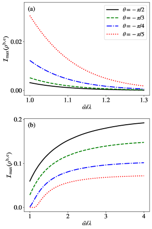
Figure 6: MLGI function $\mathcal{I}_{\text{max}}(\rho^{\text{b,e}})$ defined in (61) in terms of the mean energy splitting $\bar{\omega}$ and the detuning angle (with fixed $\lambda=1$) characterizing the asymmetry of the two-qubit system. The coupling is set as $J=0.005$. The two bosonic bath have the same (a) temperatures $T=0.1$ or (b) temperatures $T=10$.

The zeroth order of LGI function $\mathcal{I}_{+}^{(0)}(t,\rho^{\text{b,e}})$ in (69) has the maximum at $t=\pi/(3\Omega)$. And the zeroth order MLGI function is equivalent to the maximum of the zeroth order of LGI function $\mathcal{I}_{+}(t,\rho^{\text{b,e}})$. We can safely approximate the first order of MLGI function $\mathcal{I}_{\text{max}}(\rho^{\text{b,e}})$ defined in (61) by the first order of the LGI function $\mathcal{I}_{+}(t,\rho^{\text{b,e}})$ at $t=\pi/(3\Omega)$:

$$\mathcal{I}^{(1)}_{\text{max}}(\rho^{\text{b,e}})\approx\mathcal{I}_{+}^{(1)}(t=\pi/(3\Omega),\rho^{\text{b,e}}),$$ (84)

which gives

$$\mathcal{I}^{(1)}_{\text{max}}(\rho^{\text{b,e}})\\ =-\frac{4\pi J}{3\Omega}\sin^{2}\theta(\rho^{\text{b,e}}_{22}+\rho^{\text{b,e}}_{33})\left(n(\omega_{1}^{\prime})+n(\omega_{2}^{\prime})+1)\right)$$ (85)

The first order $\mathcal{I}^{(1)}_{\text{max}}(\rho^{\text{b,e}})$ is always negative irrespective to the bath parameters. Increasing the coupling $J$ will always decrease the MLGI function, namely moving the system towards the classical description.

To better see how the temperature $T$ affects $\mathcal{I}^{(1)}_{\text{max}}(\rho^{\text{b,e}})$, we can approximate the mean particle occupation number as

$$n(\omega^{\prime}_{1,2})\approx e^{-\omega^{\prime}_{1,2}/T}$$ (86)

if $T\ll\omega^{\prime}_{1,2}$. Then we have

$$\mathcal{I}^{(0)}_{\text{max}}(\rho^{\text{b,e}})+\mathcal{I}^{(1)}_{\text{max}}(\rho^{\text{b,e}})\approx\alpha\sin^{2}\theta\left(\frac{1}{2}-\frac{4\pi J}{3\Omega}\right)$$ (87)

with

$$\alpha=2e^{-\bar{\omega}/T}\cosh\left(\frac{\Omega}{2T}\right)$$ (88)

Here, the parameter $\alpha$ has the physical meaning: proportional to the population term, i.e., $\alpha\propto(\rho^{\text{b,e}}_{22}+\rho^{\text{b,e}}_{33})$. Increasing the temperature $T$ (when $T\ll\omega^{\prime}_{1,2}$) gives the LGI violation enhancement. Approximately zero temperature does not have LGI violation because the system will always be in the ground state $|1\rangle$, and the time evolution of the ground state is trivial. The population of excited states is the key for the LGIs violations. If we do not have the non-local ground state, but have non-local excited state, then the bath temperature, which gives the excitation, is beneficial for enhancing the LGIs violations.

High temperature environment deteriorates the quantumness of the system and the LGIs are expected to be preserved. For example, if the temperature is around $T\sim 10\omega^{\prime}_{1,2}$ (approximation condition in (80) can still be valid), this gives almost even distribution of the populations, see (50). Further increasing the temperature does not increase the population sum $\rho^{\text{b,e}}_{22}+\rho^{\text{b,e}}_{33}$. However, increasing the temperature (when $T\sim 10\omega^{\prime}_{1,2}$) will dramatically increase $n(\omega_{1}^{\prime})+n(\omega_{2}^{\prime})$ and therefore the first order correction $\mathcal{I}^{(1)}_{\text{max}}(\rho^{\text{b,e}})$ in (85) will decrease. At intermediate temperature $T\sim\omega^{\prime}_{1,2}$, the MLGI function $\mathcal{I}_{\text{max}}(\rho^{\text{b,e}})$ is compromised between the non-local state population and the decoherence. We can numerically explore the non-monotonic relation between $\mathcal{I}_{\text{max}}(\rho^{\text{b,e}})$ and temperature $T$, see FIG. 5. We can also check the monotonic relation between $\mathcal{I}_{\text{max}}(\rho^{\text{b,e}})$ and the coupling $J$, see FIG. 5. Stronger coupling $J$ leads to that the environment destroys the coherence (in energy basis) faster. Increasing the temperature can lead to both the excited nonlocal states and the decoherence effect, giving rise to a non-monotonic behavior.

When the two qubits have different transition frequencies $\Delta\omega\neq 0$, the eigenstates $|2\rangle$ and $|3\rangle$ (defined in Eq. (III.1)) will become less entangled. The detuning angle $\theta$ in (20) is $\theta=-\pi/2$ when $\Delta\omega=0$. Turning off the coupling of the two qubit systems ($\lambda=0$) leads to the classical descriptions (probabilistic equation) of the time evolution of the system. The inter-qubit coupling strength $\lambda$ has the monotonic relation with the MLGI function $\mathcal{I}_{\text{max}}(\rho^{\text{b,e}})$ (smaller $\lambda$ gives smaller $\mathcal{I}_{\text{max}}(\rho^{\text{b,e}})$). However, $\mathcal{I}_{\text{max}}(\rho^{\text{b,e}})$ does not have a monotonic relation with $\Delta\omega$ (changing $\theta$ with fixed $\lambda$), see FIG. 6.

Recall that in the low temperature regime ($T\ll\omega^{\prime}_{1,2}$), the MLGI function up to the first order of $J$ has the form (87), where $\alpha$ is proportional to the population term. If we increase the transition frequency difference $\Delta\omega$ (with fixed average $\bar{\omega}$), the oscillation frequency $\Omega$ in (43) will increase. Then $\alpha$ is larger with larger $\Omega$. In other words, we can increase the population sum $\rho^{\text{b,e}}_{22}+\rho^{\text{b,e}}_{33}$ by increasing the frequency difference $\Delta\omega$. In a more intuitive understanding, if the ground state is dominated, population $\rho^{\text{b,e}}_{22}$ will increase if we lower the energy level of state $|2\rangle$. Note that the eigenstate $|2\rangle$ has the energy $\omega_{1}^{\prime}=\bar{\omega}-\sqrt{\Delta\omega^{2}+\lambda^{2}}/2$. Besides, we can enhance the MLGI function in the low temperature regime by lowering the average frequency $\bar{\omega}$ (which is physically equivalent to increase the equilibrium temperature of the two baths). See the numerical results in FIG. 6 which are consistent with the analytical arguments.

If the equilibrium temperature $T$ is high ($T\gg\omega^{\prime}_{1,2}$), the population sum $\rho^{\text{b,e}}_{22}+\rho^{\text{b,e}}_{33}$ is saturated around $1/2$. The overall factor $\sin^{2}\theta$ is dominated in $\mathcal{I}_{\text{max}}^{(1)}(\rho^{\text{b,e}})$ with the expression in (85). Decreasing $\Delta\omega$ with fixed $\lambda$ or increasing $\lambda$ with fixed $\Delta\omega$ will both enhance $\mathcal{I}_{\text{max}}(\rho^{\text{b,e}})$. The more physical intuitive explanation is that the maximal entangled nonlocal states violate the local realism maximally (because the local states have the classical time evolution). Therefore, we want both qubits to have the same frequencies in order to form the Bell-type eigenstates. Also in high temperature case, lowering temperature is beneficial to test LGI violation, see FIG. 5. Then we can enhance $\mathcal{I}_{\text{max}}(\rho^{\text{b,e}})$ by increasing the mean energy splitting $\bar{\omega}$. We numerically checked the above arguments, see FIG. 6.

IV.3.2 Equilibrium fermionic Bath

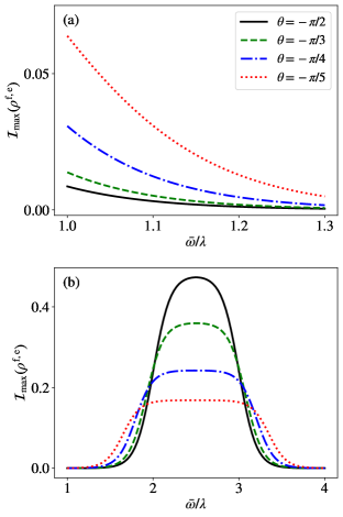
Figure 7: The MLGI function $\mathcal{I}_{\text{max}}(\rho^{\text{b,e}})$ defined in (61) in terms of the mean energy splitting $\bar{\omega}$ and the detuning angle (with fixed $\lambda=1$) characterizing the asymmetry of the two-qubit system. The coupling is set as $J=0.005$. And the temperature is $T=0.1$. The two fermionic baths have the same (a) chemical potential $\mu=0.1$ or (b) $\mu=2.5$.

We study the LGIs violations in two-qubit system (toy model of double quantum dots) coupled with equilibrium fermionic environments. We limit in the low-temperature regimes in following parts (for the fermionic environments). Similar to the equilibrium bosonic case, population space and coherent space in energy basis are decoupled in the Bloch-Redfield equation (26), which implies the commutative relation (81). Note that the time-evolution matrix $\mathcal{M}$ defined in (32) has different matrix elements for bosonic and fermionic setups, because of difference in Bose-Einstein distribution and Fermi-Dirac distribution.

In the first order coupling constant $J$, the LGI function $\mathcal{I}_{+}(t,\rho^{\text{f,e}})$ (10) has the form

$$\mathcal{I}_{+}^{(1)}(t,\rho^{\text{f,e}})=4tJ\sin^{2}\theta(\rho^{\text{f,e}}_{22}+\rho^{\text{f,e}}_{33})(\cos(2\Omega t)-\cos(\Omega t))$$ (89)

The steady state $\rho^{\text{f,e}}$ has the form in (III.3.2). We can safely approximate the first order MLGI function $\mathcal{I}_{\text{max}}(\rho^{\text{f,e}})$ defined in (61) by

$$\mathcal{I}^{(1)}_{\text{max}}(\rho^{\text{f,e}}) \approx\mathcal{I}_{+}^{(1)}(t=\pi/(3\Omega),\rho^{\text{f,e}})$$

$$=-\frac{4\pi J}{3\Omega}\sin^{2}\theta(\rho^{\text{f,e}}_{22}+\rho^{\text{f,e}}_{33})$$ (90)

Note that the zeroth order of LGI function $\mathcal{I}^{(0)}_{+}(t,\rho^{\text{f,e}})$ has a maximum at $t=\pi/(3\Omega)$ and the zeroth order of MLGI function is equivalent to the maximum of the zeroth order of LGI function $\mathcal{I}_{+}(t,\rho^{\text{f,e}})$.

The first order correction $\mathcal{I}^{(1)}_{\text{max}}(\rho^{\text{f,e}})$ is always negative. Both the zeroth and the first order of MLGI function are even functions of $\bar{\omega}-\mu$, indicating local minimum or maximum at $\mu=\bar{\omega}$. If $T\ll\bar{\omega}$ (the low temperature regime), we have the population sum

$$\rho^{\text{f,e}}_{22}+\rho^{\text{f,e}}_{33}\approx\frac{1}{\exp\left(\frac{2|\bar{\omega}-\mu|-\Omega}{2T}\right)+1}$$ (91)

The resonant point $\bar{\omega}=\mu$ gives the maximal population of the nonlocal states (eigenstates $|2\rangle$ and $|3\rangle$ are entangled states). The ground state has the particle occupation number 0; the first and the second excited states have the particle occupation number 1 and the highest excited state has the particle occupation number 2. At the resonant point $\bar{\omega}=\mu$, the system is driven into the first and the second excited states. Therefore the zeroth order of the MLGI function (74) has the global maximum at $\bar{\omega}=\mu$. Low chemical potential reservoir can not pump electrons into dots (described by the state $|1\rangle$); but high chemical potential reservoir makes all dots occupied (described by the state $|4\rangle$). Both the evolutions of states $|1\rangle$ and $|4\rangle$ admit local realism descriptions. See FIG. 5 for the numerical results of $\mathcal{I}_{\text{max}}(\rho^{\text{f,e}})$ in terms of the coupling constant and the chemical potential $\mu$.

When the ground state is dominated (two empty sites), we can increase the population sum of the first and the second excited states by lowering the mean energy splitting $\bar{\omega}$ or increasing the local energy level difference $\Delta\omega$. We can reversely argue the high chemical potential case. The above arguments are similar to the bosonic case. Consider the intermediate chemical potential regime $\mu\sim\bar{\omega}$: population sum of the first and the second excited state is almost saturated. Then changing the energy difference $\Delta\omega$ does not affect the population sum of states $|2\rangle$ and $|3\rangle$. However, states $|2\rangle$ and $|3\rangle$ will become less entangled (more local). Then we always have larger MLGI function $\mathcal{I}_{\text{max}}(\rho^{\text{b,e}})$ in (61) when $\theta=-\pi/2$, see the numerical results in FIG. 7. On the contrary, away from the resonant point $\mu\sim\bar{\omega}$, we always have MLGI $\mathcal{I}_{\text{max}}(\rho^{\text{b,e}})$ enhancement by increasing the local energy level difference $\Delta\omega$, although we have less entangled excited states.

V Legget-Garg inequalities violations in the nonequilibrium cases

In this section, we explore how the nonequilibrium condition, characterized by the temperature difference $\Delta T=T_{2}-T_{1}$ for the bosonic bath or chemical potential difference $\Delta\mu=\mu_{2}-\mu_{1}$ for the fermionic bath, contributes to the violation of LGIs. The nonequilibrium environment suggests the heat or particle current flowing through the system Castillo et al. (2013); Zhang and Wang (2014); Wang et al. (2018); Quiroga et al. (2007); Wu and Segal (2011); Dhar et al. (2012); Zhang and Wang (2015); Wang et al. (2019); Wang and Wang (2019). Consequently, there will be nonzero thermodynamic dissipation characterized by the entropy production rate Zhang and Wang (2014, 2015). Violations of the LGIs given by the nonequilibrium steady state also imply the quantum transport phenomenon Lambert et al. (2010). Firstly, we show that the heat or particle current and entropy production rate through the system increases monotonically in terms of the environment bias (temperature difference $\Delta T$ or chemical potential difference $\Delta\mu$). Then analytically, we derive the LGI function $\mathcal{I}_{+}(t,\rho^{\text{ss}})$ defined in (10) in the first order of coupling constant $J$ (approximation valid by the condition (80)). Based on that, we give analytical analysis on the first order of the MLGI function $\mathcal{I}_{\text{max}}(\rho^{\text{ss}})$ in (61) in the nonequilibrium cases. We numerically check the analytical results and numerically explore the relative high-temperature cases.

V.1 Heat/Particle Current and Entropy Production Rate

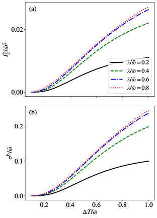
Figure 8: (a) Heat current $I_{2}^{\text{b}}$ defined in (93) and (b) entropy production rate $\sigma^{\text{b}}$ defined in (95) at steady state in terms of the nonequilibrium condition $\Delta T=T_{2}-T_{1}$ with fixed $T_{1}=0.1\bar{\omega}$. Parameters are set as $\theta=-\pi/2$ and $J=0.1\bar{\omega}$.

When the system reaches the steady state (under nonequilibrium environments), there is a constant heat or particle current flowing through the system (from the high temperature or chemical potential bath to the low temperature or chemical potential bath). The heat current is characterized by the energy change with the two environments. We have

$$\mathrm{Tr}\left(\frac{d\rho}{dt}H_{S}\right)=\sum_{l=1}^{2}I^{\text{b}}_{l}$$ (92)

where $I^{\text{b}}_{l}$ with $l=1,2$ are the heat currents through the bath 1 or 2. Superscript b reminds that we have bosonic environments. Positive $I^{\text{b}}_{l}$ means that the heat current is flowing into the system. According to the Bloch-Redfield equation (26), the heat currents are related with dissipators:

$$I^{\text{b}}_{l}=\mathrm{Tr}(\mathcal{D}_{l}[\rho]H_{S})$$ (93)

Steady state means that the energy of the system does not change. Therefore the two currents have the same magnitude but different directions:

$$I^{\text{b}}_{1}+I^{\text{b}}_{2}=0$$ (94)

If $T_{2}>T_{1}$, we have $I^{\text{b}}_{2}>0$ and $I^{\text{b}}_{1}<0$.

Given by the analytical results of the nonequilibrium steady state $\rho^{\text{b}}$, see (41a)-(41d) and (46), we can find the steady state heat current. We give the analytical steady state heat current in Appendix C. We plot the heat current $I^{\text{b}}_{2}$ in terms of the nonequilibrium condition $\Delta T=T_{2}-T_{1}$ (with fixed $T_{1}$) in FIG. 8. The current magnitude increases monotonically with the temperature bias $\Delta T$. The inter-qubit coupling (characterized by strength $\lambda$) plays an important role in heat transport Wang et al. (2018, 2019); Wang and Wang (2019). As $\lambda=0$, the two-qubit system is decoupled and the two environments are separated. No heat current flows through the system. Increasing the inter-qubit coupling strength $\lambda$ can enhance the heat flow, see FIG. 8.

Since the two reservoirs are assumed to be infinitely large compared with system, the steady state can be maintained for a very long time. We assume that the equilibrium temperatures of the two baths are always constant. The nonzero constant heat transfer at steady state implies that we have constant entropy production rate defined as

$$\sigma^{\text{b}}=-\frac{I_{1}^{\text{b}}}{T_{1}}-\frac{I_{2}^{\text{b}}}{T_{2}}=I_{2}^{\text{b}}\left(\frac{1}{T_{1}}-\frac{1}{T_{2}}\right)$$ (95)

The same magnitude $|\Delta T|$ gives the same entropy production rate $\sigma^{\text{b}}>0$. The entropy production rate also monotonically increases with nonequilibrium condition, see FIG. 8. The stronger inter-qubit coupling gives larger entropy production rate, since we have larger steady-state heat current. At far from equilibrium case, for example $T_{1}\rightarrow 0$ and $T_{2}\rightarrow\infty$, the entropy production rate is proportional to the heat current:

$$\sigma^{\text{b}}\approx\frac{I_{2}^{\text{b}}}{T_{1}}$$ (96)

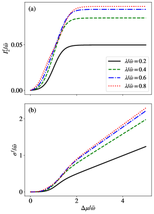
Figure 9: (a) Particle current $I_{2}^{\text{f}}$ defined in (97) and (b) entropy production rate $\sigma^{\text{f}}$ defined in (100) at steady state in terms of the nonequilibrium condition $\Delta\mu=\mu_{2}-\mu_{1}$ with fixed $\mu_{1}=0$. The two baths have the same temperatures $T_{1}=T_{2}=0.2\bar{\omega}$. Parameters are set as $\theta=-\pi/2$ and $J=0.1\bar{\omega}$.

Nonequilibrium fermionic environments suggest particle current flowing through the system. We can keep track of the particle number change in the system to reveal the particle current. Similarly with heat current, we define the particle current with respect to the two baths as

$$I^{\text{f}}_{l}=\mathrm{Tr}(\mathcal{D}_{l}[\rho]N_{S})$$ (97)

with the particle operator $N_{S}$ in energy basis $N_{S}=|2\rangle\langle 2|+|3\rangle\langle 3|+2|4\rangle\langle 4|$. The steady state gives

$$I^{\text{f}}_{1}+I^{\text{f}}_{2}=0$$ (98)

The positive current means that the electron flows into the system. The analytical expression of the particle current is given in Appendix C. We plot the particle current in terms of the chemical potential difference $\Delta\mu=\mu_{2}-\mu_{1}$ with fixed $\mu_{1}$ in FIG. 9. Due to the Pauli exclusion principle (particle occupation number $n(\omega)$ (30) is less than 1), the particle current becomes saturated when we have large chemical potential bias. For example, at relative low temperature regime $T\ll\bar{\omega}$, if $\mu_{1}\rightarrow 0$ and $\mu_{2}\rightarrow\infty$, we have the particle current

$$I_{2}^{\text{f}}\approx J(1+\rho^{\text{f}}_{23}+\rho^{\text{f}}_{32})=J\left(1-\frac{1}{1+\left(\lambda/2J\right)^{2}}\right)$$ (99)

assuming $\omega_{1}=\omega_{2}$ and constant symmetric coupling spectral $J$ (38). The current is proportional to the coherence in the energy basis. The particle current is bounded by $J$. Increasing the inter-qubit coupling gives larger particle current as expected, see FIG. 9.

The two fermionic environments are characterized by the (different) equilibrium chemical potentials and the temperatures respectively at the steady state. The entropy production rate of the environments is

$$\sigma^{\text{f}}=\frac{\mu_{1}I_{1}^{\text{f}}}{T}+\frac{\mu_{2}I_{2}^{\text{f}}}{T}=\frac{\mu_{2}-\mu_{1}}{T}I_{2}^{\text{f}}$$ (100)

Here for simplicity, we assume the same temperatures $T=T_{1}=T_{2}$ of the two baths to explore how chemical potential difference influences the dynamics and thermodynamic dissipation. At far from equilibrium case, the particle current is saturated. Therefore the entropy production rate increases linearly with the nonequilibrium condition $\Delta\mu=\mu_{2}-\mu_{1}$, see FIG. 9.

V.2 MLGI Enhanced by the Nonequilibrium bosonic Environments

In Liouville space, the time-evolution operator is given by $e^{\mathcal{M}t}$ with the matrix elements in (A)-(A), see (75). When we have nonzero nonequilibrium condition $\Delta T$, the density matrix in population space and coherence space is not decoupled, unlike the equilibrium case. Therefore, the steady state coherence in the eigenstate representation can survive in nonequilibrium environments Li et al. (2015); Wang et al. (2018, 2019). The time-evolution matrix $\mathcal{M}$ can be decomposed into coherent evolution part $\mathcal{M}_{0}$ and the dissipation part $\mathcal{M}_{J}$, see (76). These two parts do not commute in the nonequilibrium cases. As a result, the Zassenhaus formula in the first order $\mathcal{M}_{J}$ in (78) will have summation for infinite series. Fortunately, the sum has the closed form due to the simple structure of $\mathcal{M}_{0}$. For simplicity, we consider the symmetric qubit $\omega_{1}=\omega_{2}$ in the following analytical study.

The zeroth order of the LGI function $\mathcal{I}_{2}(t,\rho^{\text{ss}})$ has the contribution from the steady state coherence. Thus the nonzero steady state coherence may suggest that the two-time LGIs are violated. In the symmetric qubit setting, the inequality $\mathcal{I}^{(0)}_{2}(t,\rho^{\text{ss}})>1$ can be rewritten into

$$\rho_{44}<\mathrm{Re}\rho_{23},$$ (101)

which is possible in some nonequilibrium cases. Note that the nonequilibrium steady state coherence is proportional to the coupling constant $J$, see Eq. (46) and Eq. (53). Therefore, the inequality in Eq.(101) also implies that the possible violation of two-time LGIs is in the order $J$. We numerically check to see that the possible violation from the coherent evolution is wiped out when the nonunitary evolution is included. In the following, we concentrate on the LGI function $\mathcal{I}_{+}(t,\rho^{\text{ss}})$ defined in (10). Note that the violation by the LGI function $\mathcal{I}_{+}(t,\rho^{\text{ss}})$ is always smaller than the LGI function $\mathcal{I}_{-}(t,\rho^{\text{ss}})$ in the coherent evolution, see Eq.(71)-(72).

We obtain the first order LGI function $\mathcal{I}_{+}(t,\rho^{\text{b}})$ with the nonequilibrium corrections:

$$\mathcal{I}_{+}^{(1)}(t,\rho^{\text{b}})=4tJ(\rho^{\text{b}}_{22}+\rho^{\text{b}}_{33})\left(\tilde{n}_{1}+\tilde{n}_{2}+1)\right)(\cos(2\lambda t)-\cos(\lambda t))+\frac{2J}{\lambda}\left(\Delta n_{1}+\Delta n_{2}\right)(\sin(2\lambda t)-2\sin(\lambda t))$$ (102)

The steady state $\rho^{\text{b}}$ has the analytical solution in (41a)-(41d). The first term is the equilibrium correction (with $\sin^{2}\theta=1$), see (83). To better see how the nonequilibrium condition affects the LGIs violations, we approximate the MLGI function $\mathcal{I}_{\text{max}}(\rho^{\text{b}})$ as (same as the equilibrium case):

$$\mathcal{I}^{(1)}_{\text{max}}(\rho^{\text{b}}) \approx\mathcal{I}_{+}^{(1)}(t=\pi/(3\lambda),\rho^{\text{b}})$$

$$=-\frac{4\pi J}{3\lambda}(\rho^{\text{b}}_{22}+\rho^{\text{b}}_{33})-\frac{\sqrt{3}J}{\lambda}(\Delta n_{1}+\Delta n_{2})$$ (103)

with $\lambda\neq 0$. Note that $\lambda=0$ (decoupled two qubit system) is trivial for the LGIs violations. The first order $\mathcal{I}^{(1)}_{\text{max}}(\rho^{\text{b}})$ is always negative irrespective to either $T_{2}>T_{1}$ or $T_{1}<T_{2}$. The second term in $\mathcal{I}^{(1)}_{\text{max}}(\rho^{\text{b}})$ is the corresponding nonequilibrium correction. Note that we also have nonequilibrium corrections in steady state solution (41a)-(41d), which is proportional to $J^{2}$ order.

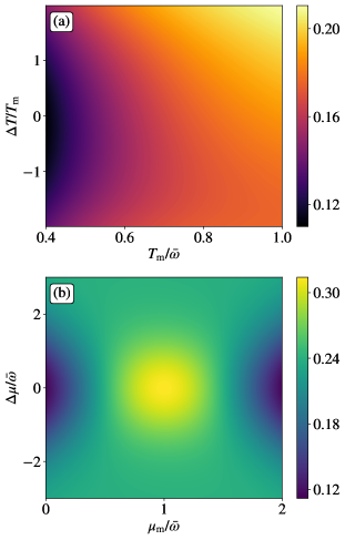
Figure 10: The contour plot diagram of MLGI function $\mathcal{I}_{\text{max}}(\rho^{\text{ss}})$ defined in (61) in terms of (a) the mean temperature $T_{\text{m}}$ and the temperature difference $\Delta T=T_{2}-T_{1}$ for the bosonic bath and (b) the mean chemical potential $\mu_{\text{m}}$ and the chemical potential difference $\Delta\mu=\mu_{2}-\mu_{1}$ for the fermionic bath with $T=0.4\bar{\omega}$. Other parameters are set as $\lambda=\bar{\omega}$, $\theta=-\pi/2$ and $J=0.005\bar{\omega}$. Red-based color is for the bosonic environment and green-based color is for the fermionic environment.

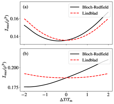
Figure 11: Comparison between the MLGI functions given by the Lindblad and the Bloch-Redfield equation. The parameters are set as $\lambda=\bar{\omega}$, $\theta=-\pi/2$ and $J=0.005\bar{\omega}$. (a) The mean temperature is relatively low $T_{\text{m}}=0.5\bar{\omega}$. (b) The mean temperature is relatively high $T_{\text{m}}=\bar{\omega}$.

The nonequilibrium correction in $\mathcal{I}^{(1)}_{\text{max}}(\rho^{\text{b}})$ is not a symmetric function of temperatures $T_{1}$ and $T_{2}$. Simple argument shows that $\Delta n_{1,2}<0$ with $T_{2}>T_{1}$. Therefore we can expect MLGI function $\mathcal{I}^{(1)}_{\text{max}}(\rho^{\text{b}})$ enhancement with $T_{2}>T_{1}$. The two-qubit system is symmetric with $T_{1}$ and $T_{2}$ if the two qubits are identical ($\omega_{1}=\omega_{2}$). In other words, the identical two qubit system has the spatial asymmetry which comes from the nonequilibrium environments. In the LGIs tests, we assume that the one-qubit system is measured locally, which introduces another asymmetry. Therefore, we expect that measuring qubit 1 will have different results with measuring qubit 2, if the two qubits are surrounded by the nonequilibrium environments $\Delta T\neq 0$. If we tune the two-qubit coupling $\lambda$ to be small, the qubit 2 coupled bath with temperature $T_{2}$ becomes another environment in terms of qubit 1. If bath 1 has high temperature, then qubit 1 becomes classical.

In the equilibrium scenario, the MLGI function $\mathcal{I}_{\text{max}}(\rho^{\text{b,e}})$ has a nonmonotonic relationship with the temperatures $T=T_{1}=T_{2}$, see FIG. 5, resulting from the competition between the nonlocal state population and the decoherence effects on the system. In the following, we fix the mean temperature and study the relationship between the MLGI function $\mathcal{I}_{\text{max}}(\rho^{\text{b}})$ and nonequilibrium condition $\Delta T=T_{2}-T_{1}$. If we have relative low mean temperature ($T_{\text{m}}\ll\bar{\omega}$ with $T_{\text{m}}=1/2(T_{1}+T_{2})$), we get the approximation:

$$\mathcal{I}_{\text{max}}^{(0)}(\rho^{\text{b}})+\mathcal{I}_{\text{max}}^{(1)}(\rho^{\text{b}})\approx\alpha^{\prime}\left(\frac{1}{2}+\frac{J}{\lambda}\left(\pm\sqrt{3}-\frac{4\pi}{3}\right)\right)$$ (104)

The plus sign is for $T_{2}>T_{1}$ and minus sign is for $T_{2}<T_{1}$. Parameter $\alpha^{\prime}$ is defined as

$$\alpha^{\prime}=e^{-\omega^{\prime}_{1}/T_{\text{eff}}}+e^{-\omega^{\prime}_{2}/T_{\text{eff}}}$$ (105)

with the effective temperature

$$T_{\text{eff}}=2T_{\text{m}}^{2}/(2T_{\text{m}}-|\Delta T|)$$ (106)

With $\Delta T=0$, the effective temperature is the equilibrium temperature $T_{\text{eff}}=T_{1}=T_{2}=T$, and $\alpha^{\prime}$ is back to the equilibrium parameter $\alpha$ defined in (88). The parameter $\alpha^{\prime}$ is approximated from the nonlocal state population sum $\rho^{\text{b}}_{22}+\rho^{\text{b}}_{33}$. We can increase $\alpha^{\prime}$ by increasing the mean temperature $\bar{T}$ or the temperature difference $\Delta T$. Therefore the increased MLGI function $\mathcal{I}_{\text{max}}(\rho^{\text{b,e}})$ via the nonequilibrium condition can be understood as the increasing nonlocal state population. Besides, the temperature difference at $T_{2}>T_{1}$ is more favorable for LGI violations than the temperature difference at $T_{2}<T_{1}$ (magnitude in the order of $J$). The asymmetric roles of $T_{1}$ and $T_{2}$ can only be characterized by the Bloch-Redfield equation. We compare the difference of the MLGI functions given by the Bloch-Redfield equation and the Lindblad respectively, see FIG. 11. Note that the Lindblad form always treats the (strongly coupled) two-qubit system collectively and therefore misses the genuine nonequilibrium effects Wang and Wang (2019).

When the mean temperature is relatively large, say $T_{\text{m}}\sim 10\bar{\omega}$, we know that the states are almost evenly distributed i.e., $\rho^{\text{b}}_{22}+\rho^{\text{b}}_{33}\approx 1/2$. Up to the first order $J$, we have

$$\mathcal{I}_{\text{max}}^{(0)}(\rho^{\text{b}})+\mathcal{I}_{\text{max}}^{(1)}(\rho^{\text{b}})\approx\\ \frac{1}{4}+\frac{J}{\lambda}\left(\left(\frac{1}{\omega^{\prime}_{1}}+\frac{1}{\omega^{\prime}_{2}}\right)\left(\frac{\sqrt{3}}{2}\Delta T-\frac{2\pi}{3}T_{\text{m}}\right)-\frac{2\pi}{3}\right)$$ (107)

We can see that $\Delta T>0$ can give LGIs violations however $\Delta T<0$ can not, see FIG. 10. Such asymmetric contribution is beyond the Lindblad description Castillo et al. (2013). See FIG. 11 for the comparison between the Lindblad and the Bloch-Redfield equation. Note that we have the same MLGI functions given by the Lindblad or the Bloch-Redfield equation if $\Delta T=0$.

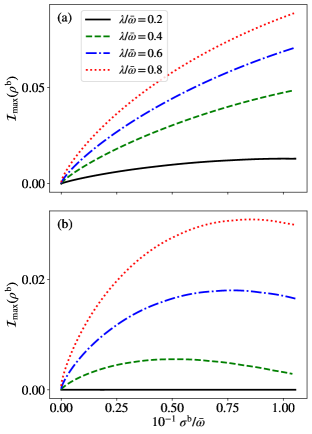
Figure 12: The MLGI function $\mathcal{I}_{\text{max}}(\rho^{\text{b}})$ defined in (61) in terms of the entropy production rate $\sigma^{\text{b}}$ defined in (95) with the different inter-qubit coupling strength $\lambda$. (a) The temperature $T_{1}$ is fixed with $T_{1}=0.1\bar{\omega}$ or (b) the temperature $T_{2}$ is fixed with $T_{2}=0.1\omega$. Other parameters are set as $\theta=-\pi/2$ and $J=0.05\bar{\omega}$.

The nonequilibrium bosonic environments have the thermodynamic cost characterized by the entropy production rate $\sigma^{\text{b}}$ defined in (95). We know that the steady state gives the constant entropy production rate which monotonically increases with the temperature difference of the two baths, see FIG. 8. The entropy production rate $\sigma^{\text{b}}$ can be viewed as another thermodynamic nonequilibrium measure, aside from the temperature difference $\Delta T$. Suppose that we fix the temperature $T_{1}$ at relatively low regime $T_{1}\ll\bar{\omega}$. The system will stay at the ground state at the equilibrium case $T_{1}=T_{2}$. Increasing the temperature $T_{2}$ will induce the heat current (at steady state) flowing from the bath 2 to the bath 1. We will have non-zero entropy production rate $\sigma^{\text{b}}$ generated from the nonequilibrium environments. The consumption in the environments characterized by the entropy production rate $\sigma^{\text{b}}$ can enhance the LGI violation if the temperature $T_{1}$ is relatively low, see FIG. 12. If we fix the temperature $T_{2}$, increasing the temperature $T_{1}$ will induce the heat current (at steady state) flowing from the bath 1 to the bath 2. The same magnitude $|\Delta T|$ gives the same entropy production rate. However, we have the stronger enhancement for the MLGI function $\mathcal{I}_{\text{max}}(\rho^{\text{b}})$ consumed by the thermodynamic cost (the nonzero entropy production rate) if $T_{1}<T_{2}$, see FIG. 12. With the same entropy production rate $\sigma^{\text{b}}$, larger inter-qubit coupling $\lambda$ gives larger MLGI function $\mathcal{I}_{\text{max}}(\rho^{\text{b}})$ either $T_{1}>T_{2}$ or $T_{1}<T_{2}$. In other words, we have more efficient thermodynamic cost (to enhance the LGI violations) if we have stronger inter-qubit coupling $\lambda$. Intuitively, stronger inter-qubit coupling $\lambda$ gives more population on the first excited state $|2\rangle$, which is nonlocal.

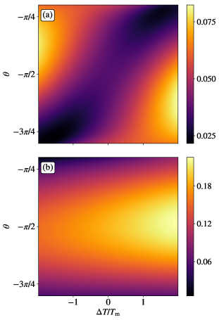
Figure 13: The MLGI function $\mathcal{I}_{\text{max}}(\rho^{\text{ss}})$ defined in (61) in terms of the nonequilibrium condition $\Delta T=T_{2}-T_{1}$ and the detuning angle $\theta$ defined in (20) with fixed $\lambda=\bar{\omega}$. (a) Mean temperature is relatively low $T_{\text{m}}=0.2\bar{\omega}$ or (b) high $T_{\text{m}}=2\bar{\omega}$. The coupling constant is set as $J=0.005\bar{\omega}$.

Detuning the qubit frequency $\Delta\omega$ can increase the MLGI function $\mathcal{I}_{\text{max}}(\rho^{\text{b,e}})$ (with equilibrium environments) if the temperature $T=T_{1}=T_{2}$ is relatively low, see FIG. 6. The relationship between the frequency difference $\Delta\omega$ and MLGI function $\mathcal{I}_{\text{max}}(\rho^{\text{b}})$ is more complicated in nonequilibrium cases. We know that the LGI function $\mathcal{I}_{\text{max}}(t,\rho^{\text{b}})$ is asymmetric in terms of temperature difference $\Delta T$. We plot the MLGI function $\mathcal{I}_{\text{max}}(\rho^{\text{b}})$ with respect to detuning angle $\theta$ defined in (20) (with fixed $\lambda$) and nonequilibrium condition $\Delta T$ in FIG. 13. When the mean temperature is relatively low $T_{\text{m}}<\bar{\omega}$, detuning $\Delta\omega>0$ or $\Delta\omega<0$ can increase MLGI function $\mathcal{I}_{\text{max}}(\rho^{\text{b}})$ with $\Delta T<0$ or $\Delta T>0$ respectively, see FIG. 13 (a). In other words, the qubit with smaller frequency should couple with higher temperature bath and vice versa. Recall that in the low mean temperature regime, the MLGI function $\mathcal{I}_{\text{max}}(\rho^{\text{b}})$ is enhanced from increasing the nonlocal state population. One can check that the nonlocal state population sum is also increased by detuning $\Delta\omega>0$ or $\Delta\omega<0$ if $\Delta T<0$ or $\Delta T>0$. Intuitively we can understand that the low frequency qubit coupled with the high temperature bath can help the excitation, since the mean temperature is relatively low and the system is at the ground state with high probability. When the mean temperature is relatively large, i.e., $T_{\text{m}}\approx\bar{\omega}$, from FIG. 13 (b), we see that detuning $\Delta\omega$ will not enhance the violations of LGIs significantly anymore for either $\Delta T>0$ or $\Delta T<0$. The asymmetric temperature contribution is obvious: $\Delta T>0$ always gives stronger enhancement of MLGI function $\mathcal{I}_{\text{max}}(\rho^{\text{b}})$. In equilibrium environments, around $T_{\text{m}}\approx\bar{\omega}$, the MLGI function $\mathcal{I}_{\text{max}}(\rho^{\text{b,e}})$ has the maximal value, see FIG. 5. Such maximal point is the result of the competition between the excitation of nonlocal states and the decoherence effect. In nonequilibrium case around $T_{\text{m}}\approx\bar{\omega}$, detuning the two qubits will not help the excitation. In fact, detuning the two qubits leads to the nonlocal state to be less entangled and therefore does not boost the LGI violation.

V.3 MLGI Enhanced by Nonequilibrium fermionic Environments

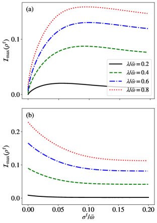
Figure 14: The MLGI function $\mathcal{I}_{\text{max}}(\rho^{\text{f}})$ defined in (61) in term of the entropy production rate $\sigma^{\text{f}}$ defined in (100) with the different inter-qubit coupling strength $\lambda$. (a) The chemical potential $\mu_{1}$ is fixed with $\mu_{1}=0$ or (b) fixed with $\mu_{1}=\bar{\omega}$. Other parameters are set as $\theta=-\pi/2$, $T_{1}=T_{2}=0.2\bar{\omega}$ and $J=0.05\bar{\omega}$.

When the two-qubit system is coupled with the two fermionic baths, we consider how the nonequilibrium condition given by $\Delta\mu=\mu_{2}-\mu_{1}$ contributes to the violations of LGIs. Same as bosonic nonequilibrium setup, the coherent evolution $\mathcal{M}_{0}$ and dissipator $\mathcal{M}_{J}$ do not commute with non-vanishing $\Delta\mu\neq 0$. However, we still can have closed form of Zassenhaus formula (78) in the first order of the coupling constant $J$. We have the first order LGI function $\mathcal{I}_{+}(t,\rho^{\text{f}})$ with the nonequilibrium corrections:

$$\mathcal{I}_{+}^{(1)}(t,\rho^{\text{f}})=4tJ(\rho^{\text{f}}_{22}+\rho^{\text{f}}_{33})(\cos(2\lambda t)-\cos(\lambda t))+\frac{2J}{\lambda}\left(\Delta n_{1}+\Delta n_{2}\right)\left(\rho^{\text{f}}_{11}-\rho^{\text{f}}_{44}\right)(\sin(2\lambda t)-2\sin(\lambda t))$$ (108)

with $\omega_{1}=\omega_{2}$ and $\lambda\neq 0$. The nonequilibrium correction term is proportional to $(\Delta n_{1}+\Delta n_{2})$. We can approximate the first order MLGI function $\mathcal{I}_{\text{max}}(\rho^{\text{b}})$ by

$$\mathcal{I}^{(1)}_{\text{max}}(\rho^{\text{f}})\approx\mathcal{I}^{(1)}(t=\pi/(3\lambda),\rho^{\text{f}}),$$ (109)

which gives

$$\mathcal{I}^{(0)}_{\text{max}}(\rho^{\text{f}})+\mathcal{I}^{(1)}_{\text{max}}(\rho^{\text{f}})=\left(\frac{1}{2}-\frac{4\pi J}{3\lambda}\right)(\rho^{\text{f}}_{22}+\rho^{\text{f}}_{33})\\ +\frac{\sqrt{3}J}{\lambda}(\Delta n_{1}+\Delta n_{2})(\rho^{\text{f}}_{44}-\rho^{\text{f}}_{11})$$ (110)

The nonequilibrium term $\Delta n_{l}$ (39c)-(39d) with $l=1,2$ is bounded $|\Delta n_{l}|<1/2$ in fermionic case. Nonequilibrium conditions $\Delta\mu>0$ and $\Delta\mu<0$ only have difference in $\mathcal{I}^{(1)}_{\text{max}}(\rho^{\text{f}})$ with magnitude in order $J$. In other words, the asymmetric nonequilibrium condition $\Delta\mu$ does not give significantly asymmetric MLGI function $\mathcal{I}_{\text{max}}(\rho^{\text{f}})$, unlike the bosonic nonequilibrium case.

In the equilibrium setup, we know that the resonant point $\bar{\mu}=\bar{\omega}$ gives the maximal MLGI. Analytically, with $\bar{\mu}=\bar{\omega}$, the population sum $\rho^{\text{f}}_{22}+\rho^{\text{f}}_{33}$ (up to first order coupling $J$) has the expression:

$$\rho^{\text{f}}_{22}+\rho^{\text{f}}_{33}=\frac{\cosh\left(\frac{\lambda}{2T}\right)}{\cosh\left(\frac{\Delta u}{2T}\right)+\cosh\left(\frac{\lambda}{2T}\right)}\\ +\frac{\sinh^{2}\left(\frac{\Delta\mu}{2T}\right)}{2\left(\cosh\left(\frac{\Delta\mu+\lambda}{2T}\right)+1\right)\left(\cosh\left(\frac{\Delta\mu-\lambda}{2T}\right)+1\right)}$$ (111)

It is easy to see that the equilibrium setup $\Delta\mu=0$ gives the maximal of population sum $\rho^{\text{f}}_{22}+\rho^{\text{f}}_{33}$. Therefore nonequilibrium condition does not give enhancement of MLGI $\mathcal{I}_{\text{max}}(\rho^{\text{f}})$ when $\bar{\mu}=\bar{\omega}$. See FIG. 10 for numerical results.

The major contribution up to the first order MLGI function in (110) is from $\rho^{\text{f}}_{22}+\rho^{\text{f}}_{33}$, which is the population sum of the non-local eigenstates. Away from the resonant point $\bar{\mu}=\bar{\omega}$, we can find that the population sum increases with the nonequilibrium condition $\Delta\mu$. Therefore, MLGI $\mathcal{I}_{\text{max}}(\rho^{\text{f}})$ can be enhanced by the nonequilibrium condition away from the resonant point. See FIG. 10 for numerical results that MLGI $\mathcal{I}_{\text{max}}(\rho^{\text{f}})$ can be enhanced by $\Delta\mu$ away from $\bar{\mu}=\bar{\omega}$.

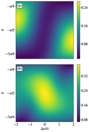
Figure 15: The MLGI function $\mathcal{I}_{\text{max}}(\rho^{\text{ss}})$ defined in (61) in terms of nonequilibrium condition $\Delta\mu=\mu_{2}-\mu_{1}$ (nonequilibrium fermionic bath with $T=0.2\bar{\omega}$) and detuning angle $\theta$ defined in (20) with fixed $\lambda=\bar{\omega}$. (a) Small mean chemical potential $\mu_{\text{m}}=0.2\bar{\omega}$ and (b) large mean chemical potential $\mu_{\text{m}}=0.8\bar{\omega}$. The coupling constant is set as $J=0.005\bar{\omega}$.

The fermionic environments with the different chemical potentials lead to the particle current flowing through the system. The nonequilibrium environments have the dissipation characterized by the entropy production rate $\sigma^{\text{f}}$ defined in (97), see FIG. 9. The MLGI function $\mathcal{I}_{\text{max}}(\rho^{\text{f}})$ can be enhanced by consuming the nonequilibrium environments (with nonzero entropy production rate $\sigma^{\text{f}}$ if the chemical potentials $\mu_{1}$ and $\mu_{2}$ are away from the resonant point $\bar{\omega}$. For example, if we fix the chemical potential $\mu_{1}$ at $\mu_{1}=0$, increasing the entropy production rate $\sigma^{\text{f}}$ gives the enhancement of LGI violation, see FIG. 14. However, if we fix the $\mu_{1}$ around the value $\bar{\omega}$, the nonequilibrium thermodynamic cost gives the smaller or zero MLGI function $\mathcal{I}_{\text{max}}(\rho^{\text{f}})$, see FIG. 14. The equilibrium case $\mu_{1}=\mu_{2}\approx\bar{\omega}$ with zero entropy production rate $\sigma^{\text{f}}$ already gives almost saturated populations $\rho_{22}^{\text{f}}+\rho_{33}^{\text{f}}$, therefore the nonequilibrium cost $\sigma^{\text{f}}$ does not enhance the LGI violation. Similarly with bosonic environments, stronger inter-qubit coupling $\lambda$ always increases the LGI violation either $\mu_{1}$ and $\mu_{2}$ away from or around the value $\bar{\omega}$.

We also studied how the detuning frequency $\Delta\omega$ combined with nonequilibrium condition $\Delta\mu$ contributes to the violations of LGIs. Numerically, we separately contour plot the two-dimensional diagram of the MLGI function $\mathcal{I}_{\text{max}}(\rho^{\text{f}})$ in terms of the nonequilibrium condition $\Delta\mu$ and the detuning angle $\theta$ (defined in (20)) with fixed tunneling strength $\lambda$, when the system is away from the resonant point or around the resonant point $\bar{\mu}=\bar{\omega}$, see FIG. (15). When the system is away $\bar{\mu}=\bar{\omega}$, the lower frequency qubit should couple the higher chemical potential reservoir and higher frequency qubit should couple the lower chemical potential reservoir, in order to reach the larger violations of LGIs. However, around the resonant point, detuning the system $\omega_{1}\neq\omega_{2}$ with nonequilibrium condition $\Delta\mu$ does not give larger violations of LGIs. The explanations are still based on the population sum $\rho^{\text{f}}_{22}+\rho^{\text{f}}_{33}$ in terms of the detuning angle $\theta$ and the nonequilibrium condition $\Delta\mu$. Away from the resonant point, the system (with high probability) stays at ground states or highest excited states which has classical description. Then detuning the two qubits by $\Delta\omega$ or by nonequilibrium condition $\Delta\mu>0$ (or $\Delta\mu<0$), we can increase the nonlocal state (the first and the second excited states) population. On the contrary, around the resonant point, the nonequilibrium condition always gives less population of nonlocal states.

VI Conclusion

We have studied the LGIs violations in a quantum system (two interacting qubits) coupled with equilibrium or nonequilibrium environments. Each qubit is coupled with one (bosonic or fermionic) bath. We have derived the evolution equation of the reduced density matrix beyond the secular approximation (Bloch-Redfield equation). There are analytical solutions of the reduced density matrix of steady states. We calculate the heat current (the system coupled with the nonequilibrium bosonic environments) or the particle current (the system coupled with the nonequilibrium fermionic environments) in the steady state regime. Correspondingly, we study the entropy production rate as the nonequilibrium thermodynamic cost. We use the maximum to LGI functions, which is called MLGI function $\mathcal{I}_{\text{max}}(\rho^{\text{ss}})$ defined in (61), to quantify the degree of the LGIs violations. We have obtained the analytical form of the two- and three-time LGI functions $\mathcal{I}_{2}(t,\rho^{\text{ss}})$ and $\mathcal{I}_{\pm}(t,\rho^{\text{ss}})$. Based on that, we analyze the MLGI function $\mathcal{I}_{\text{max}}(\rho^{\text{ss}})$ in the zeroth order and the first order of coupling $J$. The zeroth order represents the coherent evolution and the first order describes the non-unitary part (due to coupled with the environments). We also analytically separate the equilibrium and nonequilibrium effects in the first order LGI function $\mathcal{I}_{+}(t,\rho^{\text{ss}})$ and MLGI function $\mathcal{I}_{\text{max}}(\rho^{\text{ss}})$.

In the equilibrium set up, LGIs violations are caused by the unitary evolution of the first and the second excited states (entangled states in two qubit system). In the bosonic case, the MLGI function $\mathcal{I}_{\text{max}}(\rho^{\text{b,e}})$ has a non-monotonic relationship with the equilibrium temperature. The analytical results reveal that the environment can give excitation and therefore the nonlocal eigenstates (enhance the LGIs violations) but can also have decoherence effect (reduce the LGIs violations). The fermionic bath has similar results.

The nonequilibrium condition can be quantified by the temperature difference or chemical potential difference for the bosonic or fermionic reservoir respectively. The entropy production rate also characterizes the thermodynamic nonequilibrium cost. In the bosonic case, the nonequilibrium environment can magnify the violations of LGIs (increasing the MLGI function $\mathcal{I}_{\text{max}}(\rho^{\text{b}})$ by the temperature difference), if the mean temperature is relatively low. Correspondingly, the LGIs violations enhancement monotonically increases with the entropy production rate. In particular, the MLGI function $\mathcal{I}_{\text{max}}(\rho^{\text{b}})$ can be enhanced more if $T_{2}>T_{1}$ (we measure the local observable of qubit 1). Such asymmetric result is beyond the Lindblad description (wiped out by the secular approximation). In the fermionic bath setups, we have the MLGI function $\mathcal{I}_{\text{max}}(\rho^{\text{b}})$ enhancement by the nonequilibrium condition $\Delta\mu$ (chemical potential difference) if the system is away from the resonant point $\bar{\mu}=\bar{\omega}$. Such enhancement is realized by the thermodynamic nonequilibrium cost (nonzero entropy production rate). When we have the detuned two qubits (different frequencies), the low (high) frequency qubit should couple to high (low) temperature or chemical potential (with low temperature) bath in order to enhance the LGIs violations.

Whether we can realize the macroscopic coherence or Shrödinger’s cat in the experiments is a very important fundamental question in quantum mechanics. The inevitable coupling with environments leads to the decoherence (classical macrorealism description). Our study suggests new ways to test the macrorealism via the LGIs. We can take the advantage from coupling with the environments by designing nonlocal excited states of the system. Furthermore, with the detuning of the two-qubit system, the nonequilibrium environments (with different temperatures or chemical potentials) can significantly enhance the degree of the violations of LGIs. In our study, we describe quite general environments. Our results are not based on the sophisticated designed interaction between the system and the environments. It is much easier to create a system coupled with the nonequilibrium environments than a completely decoupled system. It is expected that our results can be generalized into multi-qubit system coupled with multi-nonequilibrium environments.

Appendix A Transition Matrix Elements for Time-Evolution Equation

Matrix $\mathcal{M}$ defined in (32) describing the time evolution of the system based on Bloch-Redfield equation (26) has the matrix elements $\mathcal{M}_{ab,cd}$ (with row index $ab$ and column index $cd$):

$$\mathcal{M}_{11,11}= -2\left(\cos^{2}\frac{\theta}{2}\left(\alpha_{1}(\omega_{1}^{\prime})+\alpha_{2}(\omega_{2}^{\prime})\right)\right.$$

$$+\left.\sin^{2}\frac{\theta}{2}\left(\alpha_{1}(\omega_{2}^{\prime})+\alpha_{2}(\omega_{1}^{\prime})\right)\right);$$ (112)

$$\mathcal{M}_{11,22}= \mathcal{M}_{33,44}=2\left(\cos^{2}\frac{\theta}{2}\beta_{1}(\omega_{1}^{\prime})+\sin^{2}\frac{\theta}{2}\beta_{2}(\omega_{1}^{\prime})\right);$$ (113)

$$\mathcal{M}_{11,33}= \mathcal{M}_{22,44}=2\left(\sin^{2}\frac{\theta}{2}\beta_{1}(\omega_{2}^{\prime})+\cos^{2}\frac{\theta}{2}\beta_{2}(\omega_{2}^{\prime})\right);$$ (114)

$$\mathcal{M}_{22,11}= \mathcal{M}_{44,33}=2\left(\cos^{2}\frac{\theta}{2}\alpha_{1}(\omega_{1}^{\prime})+\sin^{2}\frac{\theta}{2}\alpha_{2}(\omega_{1}^{\prime})\right);$$ (115)

$$\mathcal{M}_{22,22}= -2\left(\cos^{2}\frac{\theta}{2}\left(\beta_{1}(\omega_{1}^{\prime})+\alpha_{2}(\omega_{2}^{\prime})\right)\right.$$

$$\left.+\sin^{2}\frac{\theta}{2}\left(\alpha_{1}(\omega_{2}^{\prime})+\beta_{2}(\omega_{1}^{\prime})\right)\right);$$ (116)

$$\mathcal{M}_{33,11}= \mathcal{M}_{44,22}=2\left(\sin^{2}\frac{\theta}{2}\alpha_{1}(\omega_{2}^{\prime})+\cos^{2}\frac{\theta}{2}\alpha_{2}(\omega_{2}^{\prime})\right);$$ (117)

$$\mathcal{M}_{33,33}= -2\left(\cos^{2}\frac{\theta}{2}\left(\alpha_{1}(\omega_{1}^{\prime})+\beta_{2}(\omega_{2}^{\prime})\right)\right.$$

$$\left.+\sin^{2}\frac{\theta}{2}\left(\alpha_{2}(\omega_{1}^{\prime})+\beta_{1}(\omega_{2}^{\prime})\right)\right);$$ (118)

$$\mathcal{M}_{44,44}= -2\left(\cos^{2}\frac{\theta}{2}\left(\beta_{1}(\omega_{1}^{\prime})+\beta_{2}(\omega_{2}^{\prime})\right)\right.$$

$$\left.+\sin^{2}\frac{\theta}{2}\left(\beta_{1}(\omega_{2}^{\prime})+\beta_{2}(\omega_{1}^{\prime})\right)\right);$$ (119)

$$\mathcal{M}_{11,23}= \mathcal{M}_{11,32}=-\mathcal{M}_{23,44}=-\mathcal{M}_{32,44}$$

$$= \frac{1}{2}\sin\theta\left(\beta_{2}(\omega_{1}^{\prime})+\beta_{2}(\omega_{2}^{\prime})-\beta_{1}(\omega_{1}^{\prime})-\beta_{1}(\omega_{2}^{\prime})\right);$$ (120)

$$\mathcal{M}_{22,23}= \mathcal{M}_{22,32}=\mathcal{M}_{23,33}=\mathcal{M}_{32,33}$$

$$= \frac{1}{2}\sin\theta\left(\alpha_{2}(\omega_{1}^{\prime})+\beta_{1}(\omega_{2}^{\prime})-\alpha_{1}(\omega_{1}^{\prime})-\beta_{2}(\omega_{2}^{\prime})\right);$$ (121)

$$\mathcal{M}_{33,23}= \mathcal{M}_{33,32}=\mathcal{M}_{23,22}=\mathcal{M}_{32,22}$$

$$= \frac{1}{2}\sin\theta\left(\beta_{1}(\omega_{1}^{\prime})+\alpha_{2}(\omega_{2}^{\prime})-\alpha_{1}(\omega_{2}^{\prime})-\beta_{2}(\omega_{1}^{\prime})\right);$$ (122)

$$\mathcal{M}_{44,23}= \mathcal{M}_{44,32}=-\mathcal{M}_{23,11}=-\mathcal{M}_{32,11}$$

$$= \frac{1}{2}\sin\theta\left(\alpha_{1}(\omega_{1}^{\prime})+\alpha_{1}(\omega_{2}^{\prime})-\alpha_{2}(\omega_{1}^{\prime})-\alpha_{2}(\omega_{2}^{\prime})\right);$$ (123)

$$\mathcal{M}_{23,23}= \mathcal{M}^{*}_{23,23}=i\Omega$$

$$-(\cos^{2}\frac{\theta}{2}\left(\alpha_{1}(\omega_{1}^{\prime})+\alpha_{2}(\omega_{2}^{\prime})+\beta_{1}(\omega_{1}^{\prime})+\beta_{2}(\omega_{2}^{\prime})\right)$$

$$+\sin^{2}\frac{\theta}{2}\left(\alpha_{2}(\omega_{1}^{\prime})+\alpha_{1}(\omega_{2}^{\prime})+\beta_{2}(\omega_{1}^{\prime})+\beta_{1}(\omega_{2}^{\prime})\right))$$ (124)

$$\mathcal{M}_{11,44}= \mathcal{M}_{44,11}=\mathcal{M}_{22,33}$$

$$=\mathcal{M}_{33,22}=\mathcal{M}_{23,32}=\mathcal{M}_{32,23}=0$$ (125)

Parameters $\alpha_{l}(\omega)$ and $\beta_{l}(\omega)$ with $l=1,2$ are defined in (28). Angle $\theta$ defined in (20) tells the detuning frequency $\Delta\omega$ of the two qubits.

Appendix B Elements of Steady State Population Matrix

Steady state population matrix defined in (36) has the matrix elements when the two baths are bosonic or fermionic (with symmetric constant coupling $J_{1}(\omega)=J_{2}(\omega)=J$)

$$\mathcal{A}_{aa,bb}=\mathcal{M}_{aa,bb}+\frac{\kappa^{\text{b,f}}}{J}\mathcal{M}_{aa,23}\mathcal{M}_{23,bb}$$ (126)

with coefficient $\kappa^{\text{b}}$ for bosonic bath defined in (42) and coefficient $\kappa^{\text{f}}$ for fermionic bath defined in (52).

B.1 Elements of Steady State Population Matrix for bosonic Bath

The explicit expressions for the matrix elements $\mathcal{A}$, when the two baths are bosonic, are:

$$\mathcal{A}^{\text{b}}_{11,11}=-2\left(\tilde{n}_{1}+\tilde{n}_{2}\right)+\kappa_{b}\left(\Delta n_{1}+\Delta n_{2}\right)^{2}$$ (127)

$$\mathcal{A}^{\text{b}}_{11,22}=2\left(\tilde{n}_{1}+1\right)+\kappa_{b}\left(\Delta n_{2}^{2}-\Delta n_{1}^{2}\right)$$ (128)

$$\mathcal{A}^{\text{b}}_{11,33}=2\left(\tilde{n}_{2}+1\right)+\kappa_{b}\left(\Delta n_{1}^{2}-\Delta n_{2}^{2}\right)$$ (129)

$$\mathcal{A}^{\text{b}}_{11,44}=-\kappa_{b}\left(\Delta n_{1}+\Delta n_{2}\right)^{2}$$ (130)

$$\mathcal{A}^{\text{b}}_{22,11}=2\tilde{n}_{1}+\kappa_{b}\left(\Delta n_{1}^{2}-\Delta n_{2}^{2}\right)$$ (131)

$$\mathcal{A}^{\text{b}}_{22,22}=-2\left(\tilde{n}_{1}+\tilde{n}_{2}+1\right)-\kappa_{b}\left(\Delta n_{1}-\Delta n_{2}\right)^{2}$$ (132)

$$\mathcal{A}^{\text{b}}_{22,33}=\kappa_{b}\left(\Delta n_{1}-\Delta n_{2}\right)^{2}$$ (133)

$$\mathcal{A}^{\text{b}}_{22,44}=2\left(\tilde{n}_{2}+1\right)-\kappa_{b}\left(\Delta n_{1}^{2}-\Delta n_{2}^{2}\right)$$ (134)

$$\mathcal{A}^{\text{b}}_{33,11}=2\tilde{n}_{2}-\kappa_{b}\left(\Delta n_{1}^{2}-\Delta n_{2}^{2}\right)$$ (135)

$$\mathcal{A}^{\text{b}}_{33,22}=\kappa_{b}\left(\Delta n_{2}-\Delta n_{1}\right)^{2}$$ (136)

$$\mathcal{A}^{\text{b}}_{33,33}=-2\left(\tilde{n}_{1}+\tilde{n}_{2}+1\right)-\kappa_{b}\left(\Delta n_{1}-\Delta n_{2}\right)^{2}$$ (137)

$$\mathcal{A}^{\text{b}}_{33,44}=2\left(\tilde{n}_{1}+1\right)+\kappa_{b}\left(\Delta n_{1}^{2}-\Delta n_{2}^{2}\right)$$ (138)

$$\mathcal{A}^{\text{b}}_{44,11}=-\kappa_{b}\left(\Delta n_{1}+\Delta n_{2}\right)^{2}$$ (139)

$$\mathcal{A}^{\text{b}}_{44,22}=2\tilde{n}_{2}+\kappa_{b}\left(\Delta n_{1}^{2}-\Delta n_{2}^{2}\right)$$ (140)

$$\mathcal{A}^{\text{b}}_{44,33}=2\tilde{n}_{1}-\kappa_{b}\left(\Delta n_{1}^{2}-\Delta n_{2}^{2}\right)$$ (141)

$$\mathcal{A}^{\text{b}}_{44,44}=-2\left(\tilde{n}_{1}+\tilde{n}_{2}+2\right)+\kappa_{b}\left(\Delta n_{1}+\Delta n_{2}\right)^{2}$$ (142)

Notations $\tilde{n}_{l}$ and $\Delta$ with $l=1,2$ are defined in (39a)-(39c). Note that the overall constant $J$ in matrix $\mathcal{A}$ has omitted here.

B.2 Matrix Elements of Steady State Population Matrix for fermionic Bath

The explicit expressions for the matrix elements $\mathcal{A}$, when the two bath are fermionic, are:

$$\mathcal{A}^{\text{f}}_{11,11}=-2\left(\tilde{n}_{1}+\tilde{n}_{2}\right)+\kappa_{f}\left(\Delta n_{1}+\Delta n_{2}\right)^{2}$$ (143)

$$\mathcal{A}^{\text{f}}_{11,22}=2\left(1-\tilde{n}_{1}\right)-\kappa_{f}\left(\Delta n_{1}+\Delta n_{2}\right)^{2}$$ (144)

$$\mathcal{A}^{\text{f}}_{11,33}=2\left(1-\tilde{n}_{2}\right)-\kappa_{f}\left(\Delta n_{1}+\Delta n_{2}\right)^{2}$$ (145)

$$\mathcal{A}^{\text{f}}_{11,44}=-\kappa_{f}\left(\Delta n_{1}+\Delta n_{2}\right)^{2}$$

$$\mathcal{A}^{\text{f}}_{22,11}=2\tilde{n}_{1}+\kappa_{f}\left(\Delta n_{1}+\Delta n_{2}\right)^{2}$$ (146)

$$\mathcal{A}^{\text{f}}_{22,22}=2\left(\tilde{n}_{1}-\tilde{n}_{2}-1\right)+\kappa_{f}\left(\Delta n_{1}+\Delta n_{2}\right)^{2}$$ (147)

$$\mathcal{A}^{\text{f}}_{22,33}=+\kappa_{f}\left(\Delta n_{1}+\Delta n_{2}\right)^{2}$$ (148)

$$\mathcal{A}^{\text{f}}_{22,44}=2\left(1-\tilde{n}_{2}\right)+\kappa_{f}\left(\Delta n_{1}+\Delta n_{2}\right)^{2}$$ (149)

$$\mathcal{A}^{\text{f}}_{33,11}=2\tilde{n}_{2}+\kappa_{f}\left(\Delta n_{1}+\Delta n_{2}\right)^{2}$$ (150)

$$\mathcal{A}^{\text{f}}_{33,22}=\kappa_{f}\left(\Delta n_{1}+\Delta n_{2}\right)^{2}$$

$$\mathcal{A}^{\text{f}}_{33,33}=2\left(\tilde{n}_{2}-\tilde{n}_{1}-1\right)+\kappa_{f}\left(\Delta n_{1}+\Delta n_{2}\right)^{2}$$ (151)

$$\mathcal{A}^{\text{f}}_{33,44}=2\left(1-\tilde{n}_{1}\right)+\kappa_{f}\left(\Delta n_{1}+\Delta n_{2}\right)^{2}$$ (152)

$$\mathcal{A}^{\text{f}}_{44,11}=-\kappa_{f}\left(\Delta n_{1}+\Delta n_{2}\right)^{2}$$ (153)

$$\mathcal{A}^{\text{f}}_{44,22}=2\tilde{n}_{2}-\kappa_{f}\left(\Delta n_{1}+\Delta n_{2}\right)^{2}$$ (154)

$$\mathcal{A}^{\text{f}}_{44,33}=2\tilde{n}_{1}-\kappa_{f}\left(\Delta n_{1}+\Delta n_{2}\right)^{2}$$ (155)

$$\mathcal{A}^{\text{f}}_{44,44}=2\left(\tilde{n}_{1}+\tilde{n}_{2}-2\right)-\kappa_{f}\left(\Delta n_{1}+\Delta n_{2}\right)^{2}$$ (156)

Notations $\tilde{n}_{l}$ and $\Delta$ with $l=1,2$ are defined in (39a)-(39c).

Appendix C Steady State Heat/Particle Current

Given the steady state of nonequilibrium bosonic baths in (41a)-(41d), the heat current $I^{\text{b}}_{2}$ defined in (93) has the form

$$I^{\text{b}}_{2}= -2(\cos^{2}\frac{\theta}{2}\alpha_{1}(\omega_{1}^{\prime})\omega_{1}^{\prime}+\sin^{2}\frac{\theta}{2}\alpha_{1}(\omega_{2}^{\prime})\omega_{2}^{\prime})\rho_{11}^{\text{b}}$$

$$+2(\cos^{2}\frac{\theta}{2}\beta_{1}(\omega_{1}^{\prime})\omega_{1}^{\prime}-\sin^{2}\frac{\theta}{2}\alpha_{1}(\omega_{2}^{\prime})\omega_{2}^{\prime})\rho_{22}^{\text{b}}$$

$$+2(\sin^{2}\frac{\theta}{2}\beta_{1}(\omega_{2}^{\prime})\omega_{2}^{\prime}-\cos^{2}\frac{\theta}{2}\alpha_{1}(\omega_{1}^{\prime})\omega_{1}^{\prime})\rho_{33}^{\text{b}}$$

$$+2(\cos^{2}\frac{\theta}{2}\beta_{1}(\omega_{1}^{\prime})\omega_{1}^{\prime}+\sin^{2}\frac{\theta}{2}\beta_{1}(\omega_{2}^{\prime})\omega_{2}^{\prime})\rho_{44}^{\text{b}}$$

$$-\frac{1}{2}\sin\theta(\beta_{1}(\omega_{2}^{\prime})+\alpha_{1}(\omega_{2}^{\prime}))\omega_{1}^{\prime}(\rho^{\text{b}}_{23}+\rho^{\text{b}}_{32})$$

$$-\frac{1}{2}\sin\theta(\beta_{1}(\omega_{1}^{\prime})+\alpha_{1}(\omega_{1}^{\prime}))\omega_{2}^{\prime}(\rho^{\text{b}}_{23}+\rho^{\text{b}}_{32})$$ (157)

where the parameters $\alpha_{1}(\omega)$ and $\beta_{1}(\omega)$ are defined in (28). Note that the occupation particle number obeys the Bose-Einstein distribution.

Given the steady state of nonequilibrium fermionic baths in (51a)-(51d), the particle current $I^{\text{f}}_{2}$ defined in (97) has the form

$$I^{\text{f}}_{2}= -2(\cos^{2}\frac{\theta}{2}\alpha_{1}(\omega_{1}^{\prime})+\sin^{2}\frac{\theta}{2}\alpha_{1}(\omega_{2}^{\prime}))\rho_{11}^{\text{f}}$$

$$+2(\cos^{2}\frac{\theta}{2}\beta_{1}(\omega_{1}^{\prime})-\sin^{2}\frac{\theta}{2}\alpha_{1}(\omega_{2}^{\prime}))\rho_{22}^{\text{f}}$$

$$+2(\sin^{2}\frac{\theta}{2}\beta_{1}(\omega_{2}^{\prime})-\cos^{2}\frac{\theta}{2}\alpha_{1}(\omega_{1}^{\prime}))\rho_{33}^{\text{f}}$$

$$+2(\cos^{2}\frac{\theta}{2}\beta_{1}(\omega_{1}^{\prime})+\sin^{2}\frac{\theta}{2}\beta_{1}(\omega_{2}^{\prime}))\rho_{44}^{\text{f}}$$

$$-\frac{1}{2}\sin\theta(\beta_{1}(\omega_{2}^{\prime})+\alpha_{1}(\omega_{2}^{\prime}))(\rho^{\text{f}}_{23}+\rho^{\text{f}}_{32})$$

$$-\frac{1}{2}\sin\theta(\beta_{1}(\omega_{1}^{\prime})+\alpha_{1}(\omega_{1}^{\prime}))(\rho^{\text{f}}_{23}+\rho^{\text{f}}_{32})$$ (158)

where the parameters $\alpha_{1}(\omega)$ and $\beta_{1}(\omega)$ are defined in (28). Note that the occupation particle number obeys the Fermi-Dirac distribution.

References

- Nielsen and Chuang (2010) M. A. Nielsen and I. L. Chuang, Quantum computation and quantum information (2010).
- Horodecki et al. (2009) R. Horodecki, P. Horodecki, M. Horodecki, and K. Horodecki, Reviews of Modern Physics 81, 865 (2009).
- Modi et al. (2012) K. Modi, A. Brodutch, H. Cable, T. Paterek, and V. Vedral, Reviews of Modern Physics 84, 1655 (2012).
- Bell (1964) J. S. Bell, Physics Physique Fizika 1, 195 (1964).
- Freedman and Clauser (1972) S. J. Freedman and J. F. Clauser, Physical Review Letters 28, 938 (1972).
- Hensen et al. (2015) B. Hensen, H. Bernien, A. E. Dréau, A. Reiserer, N. Kalb, M. S. Blok, J. Ruitenberg, R. F. Vermeulen, R. N. Schouten, C. Abellán, et al., Nature 526, 682 (2015).
- Brunner et al. (2014) N. Brunner, D. Cavalcanti, S. Pironio, V. Scarani, and S. Wehner, Reviews of Modern Physics 86, 419 (2014).
- Leggett and Garg (1985) A. J. Leggett and A. Garg, Physical Review Letters 54, 857 (1985).
- Emary et al. (2013) C. Emary, N. Lambert, and F. Nori, Reports on Progress in Physics 77, 016001 (2013).
- Markiewicz et al. (2014) M. Markiewicz, P. Kurzyński, J. Thompson, S.-Y. Lee, A. Soeda, T. Paterek, and D. Kaszlikowski, Physical Review A 89, 042109 (2014).
- Fine (1982) A. Fine, Physical Review Letters 48, 291 (1982).
- Clemente and Kofler (2016) L. Clemente and J. Kofler, Physical Review Letters 116, 150401 (2016).
- Kofler and Brukner (2013) J. Kofler and Č. Brukner, Physical Review A 87, 052115 (2013).
- Saha et al. (2015) D. Saha, S. Mal, P. K. Panigrahi, and D. Home, Physical Review A 91, 032117 (2015).
- Halliwell (2016) J. Halliwell, Physical Review A 93, 022123 (2016).
- Halliwell (2017) J. Halliwell, Physical Review A 96, 012121 (2017).
- Halliwell (2019) J. Halliwell, in Journal of Physics: Conference Series, Vol. 1275 (IOP Publishing, 2019) p. 012008.
- Huelga et al. (1995) S. F. Huelga, T. W. Marshall, and E. Santos, Physical Review A 52, R2497 (1995).
- Huelga et al. (1996) S. F. Huelga, T. W. Marshall, and E. Santos, Physical Review A 54, 1798 (1996).
- Waldherr et al. (2011) G. Waldherr, P. Neumann, S. F. Huelga, F. Jelezko, and J. Wrachtrup, Physical Review Letters 107, 090401 (2011).
- Zhou et al. (2015) Z.-Q. Zhou, S. F. Huelga, C.-F. Li, and G.-C. Guo, Physical Review Letters 115, 113002 (2015).
- Formaggio et al. (2016) J. Formaggio, D. Kaiser, M. Murskyj, and T. Weiss, Physical Review Letters 117, 050402 (2016).
- Van Der Wal et al. (2000) C. H. Van Der Wal, A. Ter Haar, F. Wilhelm, R. Schouten, C. Harmans, T. Orlando, S. Lloyd, and J. Mooij, Science 290, 773 (2000).
- Palacios-Laloy et al. (2010) A. Palacios-Laloy, F. Mallet, F. Nguyen, P. Bertet, D. Vion, D. Esteve, and A. N. Korotkov, Nature Physics 6, 442 (2010).
- Goggin et al. (2011) M. Goggin, M. Almeida, M. Barbieri, B. Lanyon, J. O’brien, A. White, and G. Pryde, Proceedings of the National Academy of Sciences 108, 1256 (2011).
- Knee et al. (2012) G. C. Knee, S. Simmons, E. M. Gauger, J. J. Morton, H. Riemann, N. V. Abrosimov, P. Becker, H.-J. Pohl, K. M. Itoh, M. L. Thewalt, et al., Nature Communications 3, 606 (2012).
- Katiyar et al. (2013) H. Katiyar, A. Shukla, K. R. K. Rao, and T. Mahesh, Physical Review A 87, 052102 (2013).
- Katiyar et al. (2017) H. Katiyar, A. Brodutch, D. Lu, and R. Laflamme, New Journal of Physics 19, 023033 (2017).
- Majidy et al. (2019) S.-S. Majidy, H. Katiyar, G. Anikeeva, J. Halliwell, and R. Laflamme, Physical Review A 100, 042325 (2019).
- Wilde and Mizel (2012) M. M. Wilde and A. Mizel, Foundations of Physics 42, 256 (2012).
- Knee et al. (2016) G. C. Knee, K. Kakuyanagi, M.-C. Yeh, Y. Matsuzaki, H. Toida, H. Yamaguchi, S. Saito, A. J. Leggett, and W. J. Munro, Nature Communications 7, 1 (2016).
- Leggett et al. (1987) A. J. Leggett, S. Chakravarty, A. T. Dorsey, M. P. Fisher, A. Garg, and W. Zwerger, Reviews of Modern Physics 59, 1 (1987).
- Breuer and Petruccione (2002) H.-P. Breuer and F. Petruccione, The theory of open quantum systems (Oxford University Press on Demand, 2002).
- Zurek (2003) W. H. Zurek, Reviews of Modern Physics 75, 715 (2003).
- Scully and Zubairy (1999) M. O. Scully and M. S. Zubairy, Quantum optics (1999).
- De Vega and Alonso (2017) I. De Vega and D. Alonso, Reviews of Modern Physics 89, 015001 (2017).
- Emary (2013) C. Emary, Physical Review A 87, 032106 (2013).
- Chen et al. (2013) G.-Y. Chen, S.-L. Chen, C.-M. Li, and Y.-N. Chen, Scientific Reports 3, 2514 (2013).
- Łobejko et al. (2015) M. Łobejko, J. Łuczka, and J. Dajka, Physical Review A 91, 042113 (2015).
- Friedenberger and Lutz (2017) A. Friedenberger and E. Lutz, Physical Review A 95, 022101 (2017).
- Chanda et al. (2018) T. Chanda, T. Das, S. Mal, A. Sen, U. Sen, et al., Physical Review A 98, 022138 (2018).
- Castillo et al. (2013) J. C. Castillo, F. J. Rodríguez, and L. Quiroga, Physical Review A 88, 022104 (2013).
- Chen and Ali (2014) P.-W. Chen and M. M. Ali, Scientific Reports 4, 6165 (2014).
- Datta et al. (2018) S. Datta, S. Mal, and A. S. Majumdar, arXiv preprint arXiv:1808.10345 (2018).
- Lambert et al. (2010) N. Lambert, C. Emary, Y.-N. Chen, and F. Nori, Physical Review Letters 105, 176801 (2010).
- Addis et al. (2014) C. Addis, G. Brebner, P. Haikka, and S. Maniscalco, Physical Review A 89, 024101 (2014).
- Zhang et al. (2015) Y.-J. Zhang, W. Han, Y.-J. Xia, Y.-M. Yu, and H. Fan, Scientific Reports 5, 13359 (2015).
- Guarnieri et al. (2018) G. Guarnieri, M. Kolář, and R. Filip, Physical Review Letters 121, 070401 (2018).
- Plenio et al. (1999) M. B. Plenio, S. Huelga, A. Beige, and P. Knight, Physical Review A 59, 2468 (1999).
- Arnesen et al. (2001) M. Arnesen, S. Bose, and V. Vedral, Physical Review Letters 87, 017901 (2001).
- Wang (2001) X. Wang, Physical Review A 64, 012313 (2001).
- Kamta and Starace (2002) G. L. Kamta and A. F. Starace, Physical Review Letters 88, 107901 (2002).
- Braun (2002) D. Braun, Physical Review Letters 89, 277901 (2002).
- Benatti et al. (2003) F. Benatti, R. Floreanini, and M. Piani, Physical Review Letters 91, 070402 (2003).
- Verstraete et al. (2009) F. Verstraete, M. M. Wolf, and J. I. Cirac, Nature Physics 5, 633 (2009).
- Zhao et al. (2011) X. Zhao, J. Jing, B. Corn, and T. Yu, Physical Review A 84, 032101 (2011).
- Huelga et al. (2012) S. F. Huelga, A. Rivas, and M. B. Plenio, Physical review letters 108, 160402 (2012).
- Esposito et al. (2009) M. Esposito, U. Harbola, and S. Mukamel, Reviews of Modern Physics 81, 1665 (2009).
- Zhang and Wang (2014) Z. Zhang and J. Wang, The Journal of chemical physics 140, 245101 (2014).
- Li et al. (2015) S.-W. Li, C. Cai, and C. Sun, Annals of Physics 360, 19 (2015).
- Wang et al. (2018) Z. Wang, W. Wu, G. Cui, and J. Wang, New Journal of Physics 20, 033034 (2018).
- Lambert et al. (2007) N. Lambert, R. Aguado, and T. Brandes, Physical Review B 75, 045340 (2007).
- Quiroga et al. (2007) L. Quiroga, F. J. Rodriguez, M. E. Ramirez, and R. Paris, Physical Review A 75, 032308 (2007).
- Sinaysky et al. (2008) I. Sinaysky, F. Petruccione, and D. Burgarth, Physical Review A 78, 062301 (2008).
- Wu and Segal (2011) L.-A. Wu and D. Segal, Physical Review A 84, 012319 (2011).
- Liao et al. (2011) J.-Q. Liao, J.-F. Huang, L.-M. Kuang, et al., Physical Review A 83, 052110 (2011).
- Dhar et al. (2012) A. Dhar, K. Saito, and P. Hänggi, Physical Review E 85, 011126 (2012).
- Bellomo and Antezza (2013) B. Bellomo and M. Antezza, EPL (Europhysics Letters) 104, 10006 (2013).
- Zhang and Wang (2015) Z. Zhang and J. Wang, New Journal of Physics 17, 043053 (2015).
- Wang et al. (2019) Z. Wang, W. Wu, and J. Wang, Physical Review A 99, 042320 (2019).
- Tavakoli et al. (2018) A. Tavakoli, G. Haack, M. Huber, N. Brunner, and J. B. Brask, Quantum 2, 73 (2018).
- Tacchino et al. (2018) F. Tacchino, A. Auffèves, M. Santos, and D. Gerace, Physical Review Letters 120, 063604 (2018).
- Wang and Wang (2019) X. Wang and J. Wang, Physical Review A 100, 052331 (2019).
- Mendoza-Arenas et al. (2019) J. Mendoza-Arenas, F. Gómez-Ruiz, F. Rodríguez, and L. Quiroga, Scientific Reports 9, 1 (2019).
- Bloch (1957) F. Bloch, Physical Review 105, 1206 (1957).
- Redfield (1957) A. G. Redfield, IBM Journal of Research and Development 1, 19 (1957).
- Suárez et al. (1992) A. Suárez, R. Silbey, and I. Oppenheim, The Journal of Chemical Physics 97, 5101 (1992).
- Jeske et al. (2015) J. Jeske, D. J. Ing, M. B. Plenio, S. F. Huelga, and J. H. Cole, The Journal of Chemical Physics 142, 064104 (2015).
- Farina and Giovannetti (2019) D. Farina and V. Giovannetti, arXiv preprint arXiv:1903.07324 (2019).
- Halliwell (2014) J. Halliwell, Physics Letters A 378, 2945 (2014).
- Petrosyan and Kurizki (2002) D. Petrosyan and G. Kurizki, Physical Review Letters 89, 207902 (2002).
- Craig and Thirunamachandran (1998) D. P. Craig and T. Thirunamachandran, Molecular quantum electrodynamics: an introduction to radiation-molecule interactions (Courier Corporation, 1998).
- Lieb et al. (1961) E. Lieb, T. Schultz, and D. Mattis, Annals of Physics 16, 407 (1961).
- Hayashi et al. (2003) T. Hayashi, T. Fujisawa, H.-D. Cheong, Y. H. Jeong, and Y. Hirayama, Physical Review Letters 91, 226804 (2003).
- Sachdev (2007) S. Sachdev, Handbook of Magnetism and Advanced Magnetic Materials (2007).
- Kimura (2017) T. Kimura, Progress of Theoretical and Experimental Physics 2017 (2017).