spNNGP R package for Nearest Neighbor Gaussian Process models

Andrew O. Finley, Abhirup Datta, Sudipto Banerjee spNNGP R package for Nearest Neighbor Gaussian Process models spNNGP Nearest Neighbor Gaussian Process models This paper describes and illustrates functionality of the spNNGP R (R Core Team, 2018) package. The package provides a suite of spatial regression models for Gaussian and non-Gaussian point-referenced outcomes that are spatially indexed. The package implements several Markov chain Monte Carlo (MCMC) and MCMC-free Nearest Neighbor Gaussian Process (NNGP) models for inference about large spatial data. Non-Gaussian outcomes are modeled using a NNGP Pólya-Gamma latent variable. OpenMP parallelization options are provided to take advantage of multiprocessor systems. Package features are illustrated using simulated and real data sets. MCMC, Nearest Neighbor Gaussian Process, kriging, R MCMC, Nearest Neighbor Gaussian Process, kriging, R Andrew Finley
Department of Forestry
Michigan State University
Natural Resources Building
480 Wilson Road, Room 126
East Lansing, MI 48824-6402
E-mail:
URL: https://www.finley-lab.com

Abhirup Datta
Department of Biostatistics
Johns Hopkins Bloomberg
School of Public Health
615 N Wolfe Street, Room E3640
Baltimore, MD 21205
E-mail:
URL: http://abhidatta.com

Sudipto Banerjee
Fielding School of Public Health
University of California, Los Angeles
650 Charles E. Young Dr. South
Los Angeles, CA 90095-1772
E-mail:
URL: https://ph.ucla.edu/faculty/banerjee

1 Introduction

This paper introduces the spNNGP R (R Core Team, 2018) package that provides a suite of spatial regression models for Gaussian and non-Gaussian univariate outcomes observed at point-referenced two-dimensional locations. There are, by now, many R packages that provide similar basic functionality. A recent read of the “Analysis of Spatial Data” CRAN Task View (Bivand, 2019) yielded $\sim$46 packages listed for geostatistical analysis—and this is not an exhaustive accounting of packages available for such analyses. Our software design focus and unique contribution is to provide Bayesian models and associated diagnostic and prediction functions capable of handling data sets with a large number of locations via the Nearest Neighbor Gaussian Process (NNGP; Datta et al., 2016). Specifically, functions in spNNGP implement recent methodological and algorithmic developments presented in Finley et al. (2019).

There have been many recent methodological developments within the large spatial data literature that aim to deliver massively scalable spatial processes. Sun et al. (2011) and Banerjee (2017) provide background and discussion of current work in this area. A recent contribution by Heaton et al. (2019) is particularly useful as it provides an overview of modeling approaches for large spatial data that are under active software development, and a comparison of these approaches based on the analysis of a common dataset in the form of a “friendly competition.” In addition to NNGP models, the comparison presented by Heaton et al. (2019) considered covariance tapering via the spam package (Furrer and Sain, 2010; Furrer, 2016), gap-filling via gapfill (Gerber, 2017), metakriging (Guhaniyogi and Banerjee, 2018), spatial partitioning (Sang et al., 2011; Barbian and Assunção, 2017), fixed rank kriging via FRK (Cressie and Johannesson, 2008; Zammit-Mangion and Cressie, 2017), multiresolution approximation (Katzfuss, 2017), stochastic partial differential equations via INLA (Rue et al., 2017), lattice kriging via LatticeKrig (Nychka et al., 2015), local approximate Gaussian processes via laGP (Gramacy and Apley, 2015; Gramacy, 2016), and reduced rank predictive processes (Banerjee et al., 2008; Finley et al., 2009) via spBayes (Finley et al., 2015). The comparison was based on out-of-sampled predictive performance and, to a lesser extent, computing time for a moderately sized simulated and real dataset comprising 105,569 observations. Comparisons showed NNGP models yielded highly competitive predictive performance and computation time. More recently, Risser and Turek (2020) developed the BayesNSGP package for nonstationary Gaussian process modeling with options to use NNGPs for large data settings. In a frequentist setup, fast maximum likelihood-based parameter estimation and predictions using nearest neighbor approximations to the Gaussian Process likelihood are available in the GpGp (Guinness, 2018) and BRISC (Saha and Datta, 2018b) packages on CRAN. The latter also offers inference on the spatial covariance parameters using a fast spatial bootstrap (Saha and Datta, 2018a). While most of the software noted above exploit sparsity in the spatial covariance or precision matrix, or pursue low-rank approximations, the ExaGeoStat package (Abdulah et al., 2018) tackles decomposition of the full dense spatial covariance matrix head-on using high performance linear algebra libraries associated with various leading edge parallel architectures.

Our contribution here is many fold. We propose a novel extension for analyzing spatially correlated non-Gaussian (binary) responses using a NNGP spatial generalized linear mixed model (GLMM) by using a Pólya-Gamma prior (Polson et al., 2013) for the regression coefficients, which leads to an efficient data-augmented Gibbs sampler. This is, to our knowledge, the first sampler for Binomial spatial-GLMM that ensures closed form Gibbs updates for most parameters using linear time and storage. We discuss model comparison and model adequacy and show how different variants of the NNGP models entail fundamentally different implementation and interpretation of model comparison metrics. This is an important pragmatic consideration for practitioners choosing among different NNGP models. Finally, we provide detailed documentation and exposition of the user-friendly spNNGP R package that: 1) implements NNGP model fitting algorithms for Gaussian response spatial data presented in Datta et al. (2016) and Finley et al. (2019); 2) provides NNGP models for the non-Gaussian spatial response via the Pólya-Gamma data-augmented sampler; 3) offers support functions for NNGP model fit diagnostics, summary, and prediction. We discuss code-optimization aspects that allows spNNGP to handle very large data sets by being judicious with memory use, taking advantage of properties of the NNGP dependence scheme to efficiently store and retrieve neighbor information, and applying parallel processing where advantageous. Core model fitting and prediction functions in spNNGP have achieved unprecedented scalability, delivering inference for data sets in the hundreds of millions of spatial locations.

The remainder of this article proceeds as follows. Section 2.1 provides a brief overview of Gaussian process models followed by specifics about the NNGP models in Section 2.2. In Section 2.3 we propose extensions for Binomial spatial data and outline the Pólya-Gamma data-augmented Gibbs sampler. Section 2.4 discusses appropriate model comparison and adequacy measures for the different NNGP models. Section 2.5 gives a brief description of the code underlying spNNGP and some software development specifics for large data sets. This is followed by analysis of simulated and real data sets in Section 3 meant to provide a practical tour of some of the package’s features. Finally, Section 4 provides a brief summary with an eye toward future development.

2 Models and software

2.1 Review of Gaussian Process models for spatial data

The standard geostatistical paradigm envisions each data unit as a triplet $(\textbf{s}_{i},\textbf{x}(\textbf{s}_{i}),y(\textbf{s}_{i}))$, where $\textbf{s}_{i}$ denotes the geographical location of the measurements, $\textbf{x}(\textbf{s}_{i})$ is the $p\times 1$ vector of covariates, and $y(\textbf{s}_{i})$ is the response of interest, for $i=1,2,\ldots,n$. If the covariates fail to account for all of the structured variation observed on the response, a spatial linear mixed effects model for analyzing the data is specified as

$$y(\textbf{s}_{i})=\textbf{x}(\textbf{s}_{i})^{\top}\boldsymbol{\beta}+w(\textbf{s}_{i})+\epsilon(\textbf{s}_{i}),$$ (1)

where $\boldsymbol{\beta}$ is the $p\times 1$ vector of regression coefficients, $\epsilon(\textbf{s}_{i})$ is the random noise, customarily modeled as independent and identically distributed (iid) observations from $N(0,\tau^{2})$, and $w(\textbf{s}_{i})$ is the location-specific spatial random effect. Typically, the spatial random effects are assumed to be smooth across space, i.e., $w(\textbf{s}_{i})$ can be conceived of as realizations of a smooth latent surface $\{w(\textbf{s})\,|\,s\in\mathcal{D}\}$, where $\mathcal{D}$ denotes the geographical domain of interest. Gaussian Processes (GP) are widely used in machine learning for modeling smooth functions on the many-dimensional covariate domain (Rasmussen, 2003). For spatial regression, the mean function of the covariates is often specified parsimoniously via a linear model as in (1) and GPs are typically used to model the latent surface $w(\textbf{s})$ on the two- or three-dimensional physical domain. A GP model for the spatial surface $\{w(\textbf{s})\}$, denoted by $w(\textbf{s})\sim GP(0,C(\cdot,\cdot\,|\,{\boldsymbol{\theta}}))$ where $C(\cdot,\cdot\,|\,{\boldsymbol{\theta}})$ is a covariance function, implies that for any finite set of locations $\textbf{s}_{1},\ldots,\textbf{s}_{n}$, the vector of random effects $\textbf{w}=(w(\textbf{s}_{1}),\ldots,w(\textbf{s}_{n}))^{\top}$ follows a zero-mean multivariate Gaussian distribution with covariance matrix $\textbf{C}({\boldsymbol{\theta}})=\textbf{C}=(c_{ij})$ where $c_{ij}=C(\textbf{s}_{i},\textbf{s}_{j}\,|\,{\boldsymbol{\theta}})$. The parametric covariance function $C(\cdot,\cdot\,|\,{\boldsymbol{\theta}})$ is often selected from the Matérn family of functions (Stein, 2012), popular due to its versatility to model surfaces with varying degrees of smoothness.

The mixed effects model for the response and the GP model for the random effects can be combined into the hierarchical model

$$\textbf{y}\sim N(\textbf{X}\boldsymbol{\beta}+\textbf{w},\tau^{2}\textbf{I}),\;\textbf{w}\sim N(\textbf{0},\textbf{C}({\boldsymbol{\theta}})),$$ (2)

where y is the vector formed by stacking the $y(\textbf{s}_{i})$’s, and X is the corresponding $n\times p$ matrix of covariates. Equivalently, one can integrate out w from (2) and write

$$\textbf{y}\sim N(\textbf{X}\boldsymbol{\beta},\textbf{C}({\boldsymbol{\theta}})+\tau^{2}\textbf{I}).$$ (3)

Parameter estimation in a frequentist paradigm maximizes the likelihood from (3) with respect to $\boldsymbol{\beta}$, $\tau^{2}$ and ${\boldsymbol{\theta}}$, while in a Bayesian framework, priors are assigned to these parameters, and one can use either the hierarchical model (2) or the marginal model (3) to obtain posterior inference via Markov chain Monte Carlo (MCMC).

2.2 Nearest Neighbor Gaussian Processes for large spatial data

Gaussian Processes encounter computational roadblocks when data is observed at a large number of locations. Both the joint likelihood from the hierarchical model (2) or the data likelihood from the marginalized model (3) involves a multivariate Gaussian distribution with a dense $n\times n$ covariance matrix ($\textbf{C}({\boldsymbol{\theta}})$ and $\textbf{C}(\theta)+\tau^{2}\textbf{I}$, respectively). This task involves $O(n^{2})$ storage, and $O(n^{3})$ computations (floating point operations or FLOPs), which is infeasible when $n$ is large.

One of the scalable solutions is replacing the GP prior for the spatial random effects with a Nearest Neighbor Gaussian Process prior (Datta et al., 2016). Let $\mathcal{R}=\{\textbf{s}_{1},\ldots,\textbf{s}_{n}\}$ be any fixed finite set of locations in the spatial domain $\mathcal{D}$, and $\textbf{w}_{\mathcal{R}}=(w(\textbf{s}_{1}),\ldots,w(\textbf{s}_{n}))^{\top}$. For any location in $\mathcal{D}$, define neighbor sets as follows

$$N(\textbf{s}_{1}) =\{\}\mbox{ (empty set)},$$ (4)

$$N(\textbf{s}_{i}) =\min(m,i-1)\mbox{ nearest neighbors of }\textbf{s}_{i}\mbox{ in }\textbf{s}_{1},\ldots,\textbf{s}_{i-1},\mbox{ for }i=2,\ldots,n,$$

$$N(\textbf{s}) =m\mbox{ nearest neighbors of }\textbf{s}\mbox{ in }\mathcal{R}.$$

Then NNGP is specified as

$$\textbf{w}_{\mathcal{R}}\sim\prod_{i=1}^{n}p(w_{i}\,|\,\textbf{w}(N(\textbf{s}_{i}));\;\;w(\textbf{s})\,|\,\textbf{w}_{\mathcal{R}}\overset{ind}{\sim}p(w(\textbf{s})\,|\,\textbf{w}(N(\textbf{s}))\mbox{ for all }\textbf{s}\in\mathcal{D}\setminus\mathcal{R}.$$ (5)

In practice, $\mathcal{R}$ is chosen to be the data-locations and (5) yields the NNGP approximation to the distribution of the spatial effects. If (5) is applied to the response vector, then we obtain the likelihood approximation. This is motivated from the likelihood approximation ideas in Vecchia (1988) and Stein et al. (2004). Datta et al. (2016) showed that the above construction endows a multivariate Gaussian distribution on $\textbf{w}=\textbf{w}_{\mathcal{R}}$

$$\textbf{w}\sim N(\textbf{0},\widetilde{\textbf{C}}({\boldsymbol{\theta}}))\;,$$ (6)

where $\widetilde{\textbf{C}}({\boldsymbol{\theta}})^{-1}$, i.e., the inverse of the NNGP covariance matrix, is sparse. The extension to arbitrary locations in the bottom-row of (5) is based on kriging (conditional) distributions using only $m$-nearest neighbors from the data-locations. Nearest-neighbor kriging have been explored in Emery (2009) in the context of point-predictions as opposed to the full predictive (conditional) distributions specified for NNGP. The NNGP is itself a valid stochastic (Gaussian) process on the entire domain $\mathcal{D}$—a chief distinction from frequentist likelihood approximations or prediction equations. If probabilistic modeling of a spatial surface (observed or latent) is of primary concern, then the NNGP is a legitimate candidate and need not be viewed as an approximation of the parent GP from which it is derived. Only when inference on the spatial covariance parameters are of interest, NNGP needs to be perceived as an approximation, as these parameters describe attributes of the parent GP. The NNGP covariance function $\widetilde{C}$ is constructed from the original covariance function $C$ and ensures that the matrix $\widetilde{\textbf{C}}({\boldsymbol{\theta}})^{-1}$ is sparse and, consequently, the likelihood (6) can be evaluated using only $O(n)$ storage. This makes NNGP a scalable replacement for the full GP, while delivering inference almost indistinguishable from the full GP. NNGP can, in fact, also be looked upon as a special case of a Gaussian Markov Random Field (GMRF; Rue and Held, 2005) with a specific neighborhood structure defined through the neighbor sets of (4). In practice, however, NNGP delivers inference sufficiently close to traditional Gaussian random fields without requiring mesh-based finite element approximations of SPDE representations of Gaussian random fields (as done in Lindgren et al. (2011)).

2.2.1 Latent NNGP

The original implementation of the NNGP model proposed in Datta et al. (2016) used a fully Bayesian hierarchical specification

$$N(\textbf{y}\,|\,\textbf{X}\beta+\textbf{w},\tau^{2}\textbf{I})\times N(\textbf{w}\,|\,\textbf{0},\widetilde{\textbf{C}}({\boldsymbol{\theta}}))\times p(\boldsymbol{\beta},{\boldsymbol{\theta}},\tau^{2})$$ (7)

for running an MCMC algorithm, where all the parameters $\{\textbf{w},\boldsymbol{\beta},{\boldsymbol{\theta}},\tau^{2}\}$ are updated in a Gibbs sampler. Normal priors for $\boldsymbol{\beta}$ and inverse-Gamma priors for the variance components ensure that they produce conjugate full conditionals in the Gibbs sampler. The remaining covariance parameters are updated using random-walk Metropolis steps for their respective full conditional distributions. The full conditional distribution for w from (7) is

$$\textbf{w}\,|\,\cdot\sim N(\textbf{B}(\textbf{y}-\textbf{X}\boldsymbol{\beta})/\tau^{2}),\textbf{B})\mbox{ where }\textbf{B}=\widetilde{\textbf{C}}({\boldsymbol{\theta}})^{-1}+\textbf{I}/\tau^{2}\;.$$

Unfortunately, this block update of w is not practical. While the full conditional precision matrix $\widetilde{\textbf{C}}({\boldsymbol{\theta}})^{-1}+\textbf{I}/\tau^{2}$ has the same sparsity as $\widetilde{\textbf{C}}({\boldsymbol{\theta}})^{-1}$, unlike $\widetilde{\textbf{C}}({\boldsymbol{\theta}})^{-1}$ its determinant cannot be calculated in $O(n)$ FLOPs. Instead, Datta et al. (2016) recommended sequentially updating the full conditionals $w_{i}\,|\,\cdot$ for $i=1,\ldots,n$ and outlined an algorithm that accomplishes this entire sequence of updates in $O(n)$ FLOPs. We refer to this NNGP model as the latent NNGP.

2.2.2 Response NNGP

The latent NNGP algorithm involves running an MCMC of dimension $O(n)$ where each of the $n$ parameters $w_{i}$ are sequentially updated. While this ensures linear scalability of the NNGP model with sample size, it can also imply very slow convergence of the high-dimensional MCMC. Instead of using NNGP for the latent Gaussian process $w(\textbf{s})$, Finley et al. (2019) directly considered the marginal Gaussian process for the response, i.e., $\{y(\textbf{s})\}\sim GP(\textbf{x}(\textbf{s})^{\top}\beta,\Sigma(\cdot,\cdot))$ where the marginalized covariance function $\Sigma$ is specified as $\Sigma(\textbf{s}_{i},\textbf{s}_{j})=C(\textbf{s}_{i},\textbf{s}_{j}\,|\,{\boldsymbol{\theta}})+\tau^{2}\delta(\textbf{s}_{i},\textbf{s}_{j})$, $\delta$ denoting the Kronecker delta. Since the covariance function of an NNGP can be derived from any parent GP, Finley et al. (2019) replaced the covariance function $\Sigma$ with its NNGP analogue $\widetilde{\Sigma}$ yielding the response model

$$\textbf{Y}\sim N(\textbf{X}\boldsymbol{\beta},\widetilde{\boldsymbol{\Sigma}}),$$ (8)

where $\widetilde{\boldsymbol{\Sigma}}$ is the NNGP covariance matrix derived from $\boldsymbol{\Sigma}=\textbf{C}({\boldsymbol{\theta}})+\tau^{2}\textbf{I}$. The advantage of this response NNGP model over the previous latent model is that the dimension of the parameter space is drastically reduced from $O(n)$ to $O(1)$. The lower dimensional NNGP tends to have improved MCMC convergence as shown in Finley et al. (2019). The computational scalability per MCMC iteration of the response model remains the same as in the latent model algorithm, as $\widetilde{\boldsymbol{\Sigma}}^{-1}$ is sparse requiring $O(n)$ storage and its quadratic form and determinant can be calculated using $O(n)$ FLOPs.

2.2.3 MCMC-free inference: Conjugate NNGP model

The conjugate NNGP algorithm is an implementation of the response NNGP model which fixes certain spatial covariance parameters leading to exact (MCMC-free) posterior Bayesian inference. Recall that under the full-GP specification, the covariance function for $y(\textbf{s})$ is specified as $\Sigma(\textbf{s}_{i},\textbf{s}_{j})=C(\textbf{s}_{i},\textbf{s}_{j}\,|\,{\boldsymbol{\theta}})+\tau^{2}\delta(\textbf{s}_{i},\textbf{s}_{j})$. Usually, the covariance functions $C(\cdot,\cdot\,|\,{\boldsymbol{\theta}})$ can be expressed as $\sigma^{2}R(\cdot,\cdot\,|\,\boldsymbol{\phi})$ where $\sigma^{2}$ is the marginal variance, and $R$ is the correlation function parameterized by $\boldsymbol{\phi}$, i.e., ${\boldsymbol{\theta}}=(\sigma^{2},\boldsymbol{\phi})$. Rewriting $\tau^{2}=\alpha\sigma^{2}$, we have $\Sigma(\textbf{s}_{i},\textbf{s}_{j})=\sigma^{2}(R(\textbf{s}_{i},\textbf{s}_{j}\,|\,\boldsymbol{\phi})+\alpha\;\delta(\textbf{s}_{i},\textbf{s}_{j}))$. The conjugate NNGP model fixes $\boldsymbol{\phi}$ and $\alpha$, and generates the NNGP covariance function approximation $\widetilde{M}(\cdot,\cdot\,|\,\alpha,\boldsymbol{\phi})$ of $R(\cdot,\cdot\,|\,\boldsymbol{\phi})+\alpha\;\delta(\cdot,\cdot)$. This implies we have the following marginal model

$$\textbf{Y}\sim N(\textbf{X}\boldsymbol{\beta},\sigma^{2}\widetilde{\textbf{M}})$$ (9)

where $\widetilde{\textbf{M}}=\widetilde{\textbf{M}}(\boldsymbol{\phi},\alpha)$ is a known covariance matrix once $\boldsymbol{\phi}$ and $\alpha$ are fixed. The model in (9) is the standard Bayesian linear model with only unknowns $\boldsymbol{\beta}$ and $\sigma^{2}$. Using a Normal-Inverse-Gamma prior for ($\boldsymbol{\beta},\sigma^{2}$) leads to conjugate Normal-Inverse-Gamma posterior distributions and hence posterior moments and other summary quantities of $\boldsymbol{\beta}$ and $\sigma^{2}$ are easily and exactly obtained. Exact posterior predictive distributions for $y(\textbf{s}_{0})$ at a new location $\textbf{s}_{0}$ are also available. The matrix $\widetilde{\textbf{M}}^{-1}$ (like $\widetilde{\boldsymbol{\Sigma}}^{-1}$ for the response model) is sparse ($O(n)$) ensuring all the posterior distributions and moments can be evaluated using $O(n)$ memory and FLOPs. The fixed values of $\boldsymbol{\phi}$ and $\alpha$ are either chosen based on a variogram or can be selected in a more formal fashion using cross-validation using predictions from the model on hold-out data. We describe an implementation of the cross-validation in more detail in the MCMC-free inference subsection of Section 3. While the cross-validation enforces multiple runs of the conjugate model for a grid of values of $\boldsymbol{\phi}$ and $\alpha$, these runs can proceed in parallel. Also, $\boldsymbol{\phi}$ is usually one or two dimensional, hence, there are only 2 or 3 tuning parameters for the model and empirical results in Finley et al. (2019) suggest that a crude-resolution grid often suffices to yield accurate predictive inference. Empirical comparisons in Finley et al. (2019) and also in Heaton et al. (2019) suggest that the conjugate NNGP is orders of magnitude faster than the MCMC-based NNGP algorithms and also other competing big-spatial data methods while delivering highly competitive prediction performance.

2.3 Binomial response

All current implementations of the NNGP model assume that the response is Gaussian. Here we implement a Bayesian NNGP model for Binomial response. Note that the response and the conjugate NNGP model explicitly rely on Gaussian distributions to derive the marginal distribution for the response y. Such closed form marginal distributions are not available for non-Gaussian responses. However, conceptually we can extend the latent NNGP model of (7) to non-Gaussian settings. Assuming $y(\textbf{s}_{i})\overset{ind}{\sim}\mbox{Binomial}(n_{i},\frac{1}{1+\exp(-\psi(\textbf{s}_{i}))})$, where $\psi(\textbf{s}_{i})=\textbf{x}(\textbf{s}_{i})^{\top}\boldsymbol{\beta}+w(\textbf{s}_{i})$ with $w(\textbf{s}_{i})$ modeled as a NNGP, the joint likelihood for this model is given by:

$$\prod_{i=1}^{n}\mbox{Binomial}(y(\textbf{s}_{i})\,|\,n(\textbf{s}_{i}),\frac{1}{1+\exp(-\psi(\textbf{s}_{i}))})\times N(\textbf{w}\,|\,\textbf{0},\widetilde{\textbf{C}}({\boldsymbol{\theta}}))\times p(\boldsymbol{\beta},{\boldsymbol{\theta}})\;.$$ (10)

Since w is given an NNGP prior, this likelihood can still be evaluated using $O(n)$ memory and FLOPs. However, unlike the latent NNGP model for the Gaussian case, where the full conditional distributions $w(\textbf{s}_{i})\,|\,\cdot$ used in the Gibbs updates were Gaussian distributions, for the non-Gaussian case these full conditionals $w(\textbf{s}_{i})\,|\,\cdot$ do not belong to any standard family. Alternatively, one can resort to Metropolis-Hastings (MH) random walk updates for each $w(\textbf{s}_{i})$. Introducing $n$ MH random walk updates in every iteration would exacerbate the slow convergence issues already plaguing the latent NNGP model.

To eschew the numerous Metropolis random-walk updates, we devise a Gibbs sampler for the latent NNGP model for Binomial responses exploiting the Pólya-Gamma data-augmented sampler of Polson et al. (2013). Again, we write $\widetilde{\textbf{C}}({\boldsymbol{\theta}})=\sigma^{2}\widetilde{\textbf{R}}(\boldsymbol{\phi})$ where $\widetilde{\textbf{R}}$ is the NNGP approximation of the GP correlation matrix. We then assume a $N(\boldsymbol{\mu},\textbf{V})$ prior for $\boldsymbol{\beta}$, an $IG(a,b)$ prior for $\sigma^{2}$, and $p(\boldsymbol{\phi})$ prior for the other covariance parameters $\boldsymbol{\phi}$. Letting $\kappa(\textbf{s}_{i})=y(\textbf{s}_{i})-n(\textbf{s}_{i})/2$ we introduce the augmented data $\mbox{\boldmath$\omega$}=(\omega(\textbf{s})_{1}),\ldots,\omega(\textbf{s}_{n}))^{\top}$. We can then write the conditional likelihood

$$\begin{array}[]{cc}p(\boldsymbol{\beta},{\boldsymbol{\theta}},\textbf{w}\,|\,\textbf{y},\mbox{\boldmath$\omega$})\propto&\prod_{i=1}^{n}\exp(-\frac{\omega(\textbf{s}_{i})}{2}(\textbf{x}(\textbf{s}_{i})^{\top}\boldsymbol{\beta}+w(\textbf{s}_{i})-\kappa(\textbf{s}_{i})/\omega(\textbf{s}_{i}))^{2})\times\\ &\left(\frac{1}{\sigma^{2}}\right)^{\frac{n}{2}}\exp(-\frac{1}{2\sigma^{2}}\textbf{w}^{\top}\widetilde{\textbf{R}}(\boldsymbol{\phi})^{-1}\textbf{w})\times\\ &\exp(-\frac{1}{2}(\boldsymbol{\beta}-\boldsymbol{\mu})^{\top}\textbf{V}^{-1}(\boldsymbol{\beta}-\boldsymbol{\mu}))\times\left(\frac{1}{\sigma^{2}}\right)^{a+1}\exp(\frac{b}{\sigma^{2}})\times p(\boldsymbol{\phi}).\end{array}$$ (11)

Using the augmented data $\omega$, this likelihood for the Binomial mixed linear model is similar to the usual likelihood from a spatial mixed linear model with NNGP using responses $y(\textbf{s}_{i})^{*}=\kappa(\textbf{s}_{i})/\omega(\textbf{s}_{i})$ and heteroskedastic variances $\tau^{2}(\textbf{s}_{i})=1/\omega(\textbf{s}_{i})$.

An immediate consequence is that the updates for $\boldsymbol{\beta}$ and w are analogous to the updates in the NNGP with $y(\textbf{s}_{i})$ replaced with $y(\textbf{s}_{i})^{*}$ and the constant nugget $\tau^{2}$ replaced by $\tau^{2}(\textbf{s}_{i})$. Note that for $y(\textbf{s}_{i})^{*}$ and $\tau^{2}(\textbf{s}_{i})$ are functions of the augmented data $\omega$ and will change in every iteration. Other than that, the updates remain exactly the same as in the latent model.

The only additional update we need to do for non-Gaussian responses is that of the $\omega(\textbf{s}_{i})$’s. We update these using the full conditionals

$$\omega(\textbf{s}_{i})\sim PG(n(\textbf{s}_{i}),\textbf{x}(\textbf{s}_{i})^{\top}\boldsymbol{\beta}+w(\textbf{s}_{i}))$$

, where $PG(b,z)$ denotes the Pólya-Gamma random variable with shape parameter $b$ and tilting parameter $z$ (see Polson et al., 2013, for more details about this distribution).

This completes a Gibbs sampler for spatial GLMM with Binomial responses, where, like the Gaussian case, every parameter except the covariance parameters ($\boldsymbol{\phi}$) have closed form full conditionals. The memory requirements also remain $O(n)$ thereby ensuring that the Binomial NNGP model is a viable candidate for analysis of massive non-Gaussian spatial data.

2.4 Fitted values, replicates, and predictions

Subsequent to convergence of the MCMC for the latent or response models, we can use the posterior samples of the parameters to generate various quantities of interest like fitted values and replicates at each data location, and predictions at new locations. For the response model, samples for the fitted value of the mean at the $i^{th}$ location is simply given by $\{\textbf{x}(\textbf{s}_{i})^{\top}\boldsymbol{\beta}^{(l)}\}$ where $\boldsymbol{\beta}^{(l)}$ denotes the $l^{th}$ post burn-in sample. Similarly, for the latent NNGP, the posterior distribution of the fitted values is specified by the samples $\{\textbf{x}(\textbf{s}_{i})^{\top}\boldsymbol{\beta}^{(l)}+w(\textbf{s}_{i})^{(l)}\}$. For the MCMC-free conjugate NNGP, let $\hat{\phi}$ and $\hat{\alpha}$, respectively, denote the chosen values of $\phi$ and $\alpha$ based on cross-validation using RMSE of predictions on hold-out (test) data. Then we can express the posterior predictive distribution as a t-distribution with mean $\textbf{x}(\textbf{s}_{i})^{\top}E_{\hat{\phi},\hat{\alpha}}(\boldsymbol{\beta}\,|\,\textbf{y})$ where $E_{\hat{\phi},\hat{\alpha}}(\boldsymbol{\beta}\,|\,\textbf{y})$ denotes the posterior mean of $\boldsymbol{\beta}$ at $\phi=\hat{\phi}$ and $\alpha=\hat{\alpha}$. The closed-form expressions for $E_{\hat{\phi},\hat{\alpha}}(\boldsymbol{\beta}\,|\,\textbf{y})$ and the scale parameter for the t-distribution for the fitted value are available in Algorithm 5 of Finley et al. (2019).

Following Gelman et al. (2013) we consider generating replicate data at the observed data locations. This is often used for model checking and model adequacy evaluations and is based upon simulating each data point from its posterior predictive distribution. We note that while both the latent model (2) and the response model (3) lead to the same marginal distribution for y, the two models differ fundamentally in their definition for replicate data. For the hierarchical model, conditional on $\boldsymbol{\beta}$, ${\boldsymbol{\theta}}$ and w’s, the $y(\textbf{s}_{i})$’s are independent with iid $N(0,\tau^{2})$ distributed error terms. Hence, for each post-burn-in sample of the parameters, replicates at each data location can be generated as $\{y(\textbf{s}_{i})^{(l)}\sim N(\textbf{x}(\textbf{s}_{i})^{\top}\boldsymbol{\beta}^{(l)}+w(\textbf{s}_{i})^{(l)},{\tau^{2}}^{(l)})\}$. For the response model, however, we can think of y as a single multivariate observation from $N(\textbf{X}\beta,\boldsymbol{\Sigma})$. Things are further complicated when switching to the NNGP covariance matrix $\widetilde{\boldsymbol{\Sigma}}$ as, unlike $\boldsymbol{\Sigma}$, we cannot express $\widetilde{\boldsymbol{\Sigma}}$ as the sum of a purely spatial covariance matrix and a diagonal matrix of error variances. Hence, replicates for the marginalized model are basically new multivariate draws from $N(\textbf{X}\boldsymbol{\beta}^{(l)},\widetilde{\boldsymbol{\Sigma}}({\boldsymbol{\theta}}^{(l)}))$. Unlike the replicates from the hierarchical model, which are expected to exhibit strong spatial alignment with the observed data owing to the correlation induced through the use of the common w’s, the replicates for the response model are only correlated with the observed data through $\boldsymbol{\beta}$ and ${\boldsymbol{\theta}}$ and hence are not expected to have similar spatial contours as the observed data. For the conjugate NNGP, which also relies on the marginalized model, the replicates are draws from $N(\textbf{X}\boldsymbol{\beta}^{(l)}_{\hat{\boldsymbol{\phi}},\hat{\alpha}},{\sigma^{2}}^{(l)}_{\hat{\boldsymbol{\phi}},\hat{\alpha}}\widetilde{\textbf{M}}(\hat{\boldsymbol{\phi}},\hat{\alpha}))$ with $\{(\boldsymbol{\beta}^{(l)}_{\hat{\boldsymbol{\phi}},\hat{\alpha}},{\sigma^{2}}^{(l)}_{\hat{\boldsymbol{\phi}},\hat{\alpha}})\}$ denoting the Normal-Inverse-Gamma posterior samples of $\boldsymbol{\beta}$ and $\sigma^{2}$ at the chosen value of $\hat{\phi}$ and $\hat{\alpha}$.

Finally, we turn our attention to predictions at a new location s. For the latent model, predictions are also generated hierarchically by first generating samples of $w(\textbf{s})^{(l)}\,|\,\textbf{w}(N(\textbf{s}))^{(l)},{\boldsymbol{\theta}}^{(l)}$. This conditional distribution is Gaussian with mean and variance being the kriging mean and variance at s based on a set of nearest neighbors $N(\textbf{s})$. The exact expressions for these quantities are specified in Algorithm 2 of Finley et al. (2019). Subsequent to generating samples of $w(\textbf{s})$, we generate replicates for the response as $y(\textbf{s})^{(l)}\,|\,w(\textbf{s})^{(l)},\boldsymbol{\beta}^{(l)},{\tau^{2}}^{(l)}\sim N(\textbf{x}(\textbf{s})^{\top}\boldsymbol{\beta}^{(l)}+w(\textbf{s})^{(l)},{\tau^{2}}^{(l)})$. For the response model, the prediction algorithm is presented in Algorithm 4 of Finley et al. (2019) and involves directly generating samples of $y(\textbf{s})^{(l)}\,|\,y(N(\textbf{s})),\boldsymbol{\beta}^{(l)},{\boldsymbol{\theta}}^{(l)}$. This is once again a conditional normal distribution equivalent to kriging at s given its neighbors $N(\textbf{s})$ for the response process $y(\cdot)$. For the conjugate model, exact predictive distributions are available as $y(\textbf{s})\,|\,$data following a $t$-distribution with location and scale parameters provided in Algorithm 5 of Finley et al. (2019). Finally, for Binomial responses, predictions follow the same strategy as the latent model for Gaussian responses as both models rely on the hierarchical latent variable formulation. We initially generate samples of $w(\textbf{s})^{(l)}\,|\,\textbf{w}(N(\textbf{s}))^{(l)},{\boldsymbol{\theta}}^{(l)}$ followed by generating Binomial samples for the response as $y(\textbf{s})^{(l)}\,|\,w(\textbf{s})^{(l)},\boldsymbol{\beta}^{(l)},{\tau^{2}}^{(l)}\sim\mbox{Binomial}(n(\textbf{s}),(1+exp(-(\textbf{x}(\textbf{s})^{\top}\boldsymbol{\beta}^{(l)}+w(\textbf{s})^{(l)})))^{-1})$ where $n(\textbf{s})$ denotes the total count at s.

2.5 Software features

Two model fitting functions spNNGP and spConjNNGP, with associated support functions, offer users a set of efficient regression and prediction tools that implement the methods outlined in Sections 2.2 and 2.3. Following from Section 2.2, spNNGP provides MCMC-based inference for the latent and response spatial regression models. The latent model can be specified for Gaussian and Binomial (via the Pólya-Gamma distribution Section 2.3) outcome variables, while the response model only fits Gaussian outcome variables. The highly efficient MCMC-free conjugate NNGP algorithm used for Gaussian outcome variables described in Section 2.2 is available via the spConjNNGP function.

The spNNGP and spConjNNGP functions as well as their support functions (fitted for generating regression fitted and replicated data, spDiag for computing model diagnostics, and predict for sampling from posterior predictive distributions) are written in C/C++ using R’s foreign language interface and offer parallelization using openMP (Dagum and Menon, 1998).

As noted previously, our aim was to provide software capable of handling data sets with 10s to 100s of millions of locations. This aim was met by minimizing memory requirements, and taking advantage of parallelization where possible. We attempted to minimize memory requirements in several ways. First, we avoid making copies of input data, e.g., the regression design matrix, spatial coordinate matrix, etc. Second, we do not hold any Euclidean distance or subsequent spatial covariance vectors and matrices in memory, but rather compute them when needed. For example, all sampling algorithms require the computation of the spatial covariance vector between each observed location and its set of nearest neighbors, and the among neighbors spatial covariance matrix. For any given observation this storage requirement is not large, i.e., at most a $m$ length vector and upper or lower triangle of an $m\times m$ matrix, where $m$ is the number of neighbors (which is small, e.g., $m=15$). However, when $n$ is large, storing $n$ $m$ length vectors and $m\times m$ matrices is substantial. Therefore, we made the decision to compute these covariance vectors and matrices “on the fly” for each observation and for each iteration of the given sampler. To do this efficiently, we find each observation’s neighbor set via a fast code book search described in Ra and Kim (1993) which is modified to accommodate the ordering. The neighbor search is performed only once at the beginning of the program, and the result is $n$ vectors of at most $m$ integers that record the data row index for each observation’s neighbors (i.e., the indexes in the input outcome vector and corresponding design and coordinate matrices).

The ordering and subsequent selection of $m$-(directed) nearest neighbors can be summarized as a directed acyclic neighbor graph. This neighbor graph can be encoded as a sparse lower-triangular matrix where each row is an observation and the non-zero elements in each row hold the neighbor indexes. Within the software, this matrix is held in Compressed Row Storage (CRS) format to minimize memory use and neighbors’ data retrieval time. The CRS format does not store zeros and organizes non-zero matrix elements ordered by row in contiguous memory. This is advantageous in our setting because it makes traversing all observations’ neighbor indexes as simple as a single loop over the vector that holds the CRS matrix’s non-zero elements. Given the index for a given neighbor, retrieving its spatial coordinates, design matrix, and outcome value is further simplified because all input data are stored in contiguous memory column-major format, which allows for fast retrieval of data using integer indexing. This straightforward looping and use of integer indexing to retrieve neighbor input data facilitates parallelization using an openMP omp for pragma at several points in the sampling algorithms.

Figure 1 provides an example of a neighbor graph and the corresponding sparse matrix that we store in CRS format. Following the sampling algorithms in Datta et al. (2016) and Finley et al. (2019), the response and conjugate models require only each observation’s neighbor information; however, the latent model sampling algorithm requires information on which observations have a given observation as a neighbor. Or put another way, we need to know which neighbor sets each observation is a member of. This information is easily accessed by noting the row index of each column’s non-zero elements in Figure 1, e.g., observation 1 is in the neighbor sets for observation 2, 3, and 4. Efficiently accessing and traversing these indexes is done in the software by converting the CRS neighbor index matrix to a Compressed Column Storage (CCS) format, which effectively reorders the needed row indexes in contiguous memory by column.

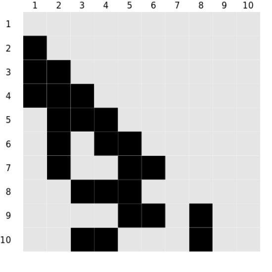
Figure 1: 1 Illustration of a neighbor graph using three neighbors for ten observations with ordering along the easting axis. 1 The sparse lower-triangular matrix (black elements are non-zero) corresponding to the graph in 1 that records the neighbor index (columns) for each observation index (rows).

Storing all vectors and matrices in contiguous memory column-major format also simplifies calls to Fortran Basic Linear Algebra Subprograms (BLAS; www.netlib.org/blas) and Linear Algebra Package (LAPACK; www.netlib.org/lapack), which are used for all computationally intensive matrix operations. Hence, additional speed-up can be realized if R calls a threaded implementation of BLAS, e.g., openBLAS (Zhang, 2016) or Intel’s Math Kernel Library (MKL) (Intel, 2019), while working on a multiple processor computer. Finley et al. (2019) provide details about where and how each sampling algorithm uses parallelization.

3 Illustrations

3.1 Analysis of simulated data

The basic functionality of spNNGP and spConjNNGP, along with their support functions, are illustrated using a small $n$=5000 simulated data set with locations distributed at random within a unit square domain. This data set was kept purposely small so the NNGP models could be compared with the full GP model. The Gaussian outcome variable was generated from (2) with latent w centered on zero and covariance matrix elements $c_{ij}=\sigma^{2}\exp(-\phi||\textbf{s}_{i}-\textbf{s}_{j}||)$, where $\phi$=6 and $\sigma^{2}$=1. The columns in the design matrix comprise an intercept and variable x which was drawn from a Normal distribution with mean zero and variance 1. The regression coefficients were $\boldsymbol{\beta}=(1,-0.1)^{\top}$ and measurement error $\tau^{2}$=0.1. An additional $n_{0}$=2500 observations on a grid were set aside to illustrate prediction.

3.1.1 MCMC-based inference

A call to spNNGP generates samples from parameters’ posterior distributions and, optionally, corresponding samples of regression fitted values and replicates via composition sampling as described in Section 2.4. Similar to R’s lm function, the desired model is passed to spNNGP via the formula argument. The model’s outcome vector and design matrix components are then found in a data frame passed to the data argument or, if data is not specified, taken from the calling environment. Additionally, the locations corresponding to the observed data are passed as a matrix via the coords argument. One can also pass coords a character vector of column names in data’s data frame.

Specifying the latent or response model is done via the method argument. As detailed in Finley et al. (2019), for the latent model (initialized by setting method="latent") $\boldsymbol{\beta}$, w, $\sigma^{2}$, and $\tau^{2}$ are updated from their respective full conditional distributions via a Gibbs algorithm. The spatial correlation function decay parameter $\phi$ and, if cov.model="matern" (where cov.model specifies the desired spatial correlation function), smoothness parameter $\nu$ are updated via a MH algorithm. If method="response", only $\boldsymbol{\beta}$ has an efficient closed form full conditional Gibbs update and the remaining parameters $\sigma^{2}$, $\tau^{2}$, $\phi$, and perhaps $\nu$ are updated via MH. For both models, starting values and prior distributions must be specified for all parameters (with the optional exception of $\boldsymbol{\beta}$ and w) via the starting and priors arguments, as illustrated below. Those parameters updated via MH are transformed to have support on the real line so that a Normal proposal distribution can be used. The variance of the parameter specific proposal distribution is controlled via the tuning argument. Tuning values should be selected to maintain the desired MH acceptance rate (in general we aim for $\sim$25-50 percent, see Roberts and Rosenthal (2009) and Gelman et al. (2013) for guidance). Information about acceptance rate and other model specifics is printed to the console when verbose=TRUE.

A NNGP model requires two user inputs: ordering of the locations, and number of nearest neighbors $m$ to use. The top-row of Equation (5) clearly depends on the ordering of the locations in $\mathcal{R}$. As defined in Equation 4, given an ordering, for a data-location corresponding to an observation, the neighbor set (conditioning set) is constructed as the set of $m$ nearest neighbors of s that conform to the user-specified ordering (i.e., directed nearest neighbors). By default, spNNGP and spConjNNGP order in increasing value of the first column of the matrix passed to coords, which, in most settings, produces an excellent approximation to a full GP (see supplemental experiments in Datta et al. (2016)); however, as demonstrated by Guinness (2018) improvements in parameter estimation efficiency can be achieved with different ordering designs. Functions to obtain these alternate orderings are provided in the GpGP R package (Guinness, 2018). If the user wishes to try different orderings, they can be passed as an integer index vector via the optional ord argument. For illustration, we bypass the default ordering in the call to spNNGP below and order using the sum of locations’ $x$ and $y$ coordinate values. We reemphasize that, subsequent to selection of any ordering, NNGP always uses nearest neighbors corresponding to that ordering. Other neighbor selection schemes such as mixture of nearest and farthest neighbors have been considered in related earlier work (Stein et al., 2004) but is not implemented in spNNGP. The number of neighbors to consider is controlled by the n.neighbors argument. As demonstrated in Datta et al. (2016) 15 neighbors is usually sufficient; however, depending on the data, one can achieve a good approximation to the full GP with as few as five neighbors. If $n$ is large, selecting fewer neighbors can result in substantial decrease in runtime.

Users can choose a slow brute force or fast code book nearest neighbor search algorithm by setting the search.type argument to "brute" or "cb", respectively. The fast code book search is a modified version of the algorithm detailed in Ra and Kim (1993). If locations do not have identical coordinate values on the axis used for the ordering then "cb" and "brute" should produce identical neighbor sets. However, if there are identical coordinate values on the axis used for ordering, then the search algorithms might produce different, but equally valid, neighbor sets. If $n$ is large (e.g., a million or more), constructing the nearest neighbor sets can take a long time even when search.type="cb". To save time, the neighbor set can be reused in subsequent model calls if the values passed to coords, ord, and n.neighbors do not change. Setting return.neighbor.info = TRUE in spNNGP or spConjNNGP returns the necessary neighbor information in an object called neighbor.info. Then passing this object to the optional neighbor.info argument in subsequent calls to spNNGP or spConjNNGP avoids the costly nearest neighbor search. The information in neighbor.info can also be used if one wishes to plot the neighbor sets (see example code in the spNNGP manual page).

The call to spNNGP in the code below generates 2000 MCMC samples using the latent model (with the n.samples argument specifying the desired number of samples). The n.report argument defines the sample interval for reporting the MH acceptance rate, which in this case is once every 1000 samples. The fit.rep=TRUE indicates that we are requesting regression fitted and replicate data be generated via composition sampling (i.e., one-for-one with each MCMC sample). The argument sub.sample specifies that we only want regression fitted and replicate samples starting at MCMC sample 1000 and for each subsequent sample, i.e., start=1000 (the list passed to sub.sample can also define end and thin for additional control over MCMC chain samples used in the computations).

The computer used to conduct this analysis has multicore processor and R compiled with openMP. Therefore, setting n.omp.threads=4 should decrease runtime, see Section 3.2 for more details on computing time.

R> n.samples <- 2000
R> starting <- list("phi"=3/0.5, "sigma.sq"=1, "tau.sq"=1)
R> priors <- list("phi.Unif"=c(3/1, 3/0.1), "sigma.sq.IG"=c(2, 1),
+   "tau.sq.IG"=c(2, 1))
R> cov.model <- "exponential"
R> tuning <- list("phi"=0.2)
R> ord <- order(coords[,1]+coords[,2])
R> sim.s <- spNNGP(formula=y~x, coords=coords, starting=starting,
+   tuning=tuning, priors=priors, cov.model=cov.model, n.samples=n.samples,
+   n.neighbors=10, method="latent", ord=ord, n.omp.threads=4,
+   n.report=1000, fit.rep=TRUE, sub.sample=list(start=1000),
+   return.neighbor.info = TRUE)

## ----------------------------------------
## ΨBuilding the neighbor list
## ----------------------------------------
## ----------------------------------------
## Building the neighbors of neighbors list
## ----------------------------------------
## ----------------------------------------
## ΨModel description
## ----------------------------------------
## NNGP Latent model fit with 5000 observations.
##
## Number of covariates 2 (including intercept if specified).
##
## Using the exponential spatial correlation model.
##
## Using 10 nearest neighbors.
##
## Number of MCMC samples 2000.
##
## Priors and hyperpriors:
## Ψbeta flat.
## Ψsigma.sq IG hyperpriors shape=2.00000 and scale=1.00000
## Ψtau.sq IG hyperpriors shape=2.00000 and scale=1.00000
## Ψphi Unif hyperpriors a=3.00000 and b=30.00000
##
## Source compiled with OpenMP support and model fit using 4 thread(s).
## ----------------------------------------
## ΨΨSampling
## ----------------------------------------
## Sampled: 1000 of 2000, 50.00%
## Report interval Metrop. Acceptance rate: 46.50%
## Overall Metrop. Acceptance rate: 46.50%
## -------------------------------------------------
## Sampled: 2000 of 2000, 100.00%
## Report interval Metrop. Acceptance rate: 33.70%
## Overall Metrop. Acceptance rate: 40.10%
## -------------------------------------------------

As seen in the output above the call to spNNGP prints some basic model and sampler information. The output also notes Source compiled with OpenMP support and model fit using 4 thread(s). spNNGP functions will throw a warning if R was not compiled with openMP support and n.omp.threads is set to a value greater than 1.

Objects returned by spNNGP and other functions in the package use S3 methods summary and print. As illustrated later, S3 methods for fitted and residuals are also implemented. The print method prints the initial call to the function as well as some model and sampler specifics. The default behavior of summary is to print posterior summaries for model parameters using samples from the second half of the MCMC chains. The values for arguments sub.sample and quantiles passed to summary allow for finer control on posterior summaries. Alternatively the user can access all posterior samples as coda (Plummer et al., 2006) mcmc class objects in the spNNGP return objects’ p.beta.samples, p.theta.samples, and p.w.samples, which as the names suggest hold $\boldsymbol{\beta}$, ${\boldsymbol{\theta}}$, and w samples, respectively.

R> summary(sim.s)

##
## Call:
## spNNGP(formula = y ~ x, coords = coords, method = "latent",
##     n.neighbors = 10, starting = starting, tuning = tuning,
##     priors = priors, cov.model = cov.model, n.samples = n.samples,
##     n.omp.threads = 4, ord = ord, return.neighbor.info = TRUE,
##     fit.rep = TRUE, sub.sample = list(start = 1000), n.report = 1000)
##
## Model class is NNGP, method latent, family gaussian.
##
## Model object contains 2000 MCMC samples.
##
## Chain sub.sample:
## start = 1000
## end = 2000
## thin = 1
## samples size = 1001
##             2.5%    25%     50%     75%     97.5%
## (Intercept) 0.5648  0.5948  0.6182  0.6757  0.7781
## x           -0.1066 -0.0966 -0.0912 -0.0852 -0.0756
## sigma.sq    0.8535  0.9446  1.0013  1.1486  1.6633
## tau.sq      0.2292  0.2378  0.2428  0.2486  0.2581
## phi         3.5656  4.7293  5.8478  6.2808  6.9279

As requested by setting fit.rep=TRUE the spNNGP return object also holds samples for the regression fitted values, labeled y.hat.samples, and replicated data, labeled y.rep.samples. For convenience, the median and lower and upper 95% credible intervals for MCMC samples at each location are provided in y.hat.quants and y.rep.quants. These samples and corresponding summaries can be accessed directly in the spNNGP return object or extracted using the S3 fitted method. Beyond simply extracting the regression fitted values and replicated data from spNNGP and other model objects in the package, the fitted function performs additional composition sampling if the requested MCMC sample subset differs from the one initially specified in the model call. For example, the initial call to spNNGP specified sub.sample=list(start=1000), but if later we decide we want regression fitted values and replicated data for every 10^th MCMC sample starting at sample 100, a call to fitted(sim.s, sub.sample=list(start=100, thin=10)) would generate the desired subset (the residuals function provides the same behavior).

3.1.2 MCMC-free inference

The conjugate model is called using the spConjNNGP function. Fixed $\alpha$, $\phi$, and perhaps $\nu$ are specified using a named vector passed to the theta.alpha argument. Alternatively, a $K$-fold cross-validation (where $K$ is set via the k-fold argument) is used to discover the “optimal” set of parameters if theta.alpha is passed a matrix with columns named alpha, phi, and perhaps nu. The “optimal” set of parameter values (i.e., a row in theta.alpha) is the one that minimizes the average value of the specified scoring rule over the $K$ folds. This scoring rule is set via the score.rule argument with options "rmspe" and "crps" for root mean squared prediction error (RMSPE) and continuous ranked probability score (CRPS; Gneiting and Raftery, 2007). The $K$-fold cross-validation progress is printed to the screen as illustrated below. Once the optimal parameter set is identified, a final model is fit using all the available data. The description of this final model is given in the Model description section followed by the optimal set of $\alpha$, $\phi$, and, if the Matérn correlation model is used, $\nu$.

The printout following the call to spConjNNGP below also includes a section called Computing replicates that reports on the exact sampling from the model parameters and regression fitted values posterior distributions, and generation of replicated data. Posterior sampling and generation of replicated data is optional and controlled by the fit.rep and n.samples arguments, with n.samples being set to the number of desired samples to collect. When fit.rep=TRUE, spConjNNGP effectively calls the S3 method fitted function for the conjugate model class. Hence, if posterior samples are not collected in the initial call to spConjNNGP or a different number of samples is needed, then a call to fitted using the spConjNNGP object will generate the required samples.

R> theta.alpha <- as.matrix(expand.grid(seq(0.01,1,length.out=15),
+   seq(3,30,length.out=15)))
R> colnames(theta.alpha) <- c("alpha","phi")
R> sim.c <- spConjNNGP(y~x, coords=as.matrix(coords),
+   cov.model="exponential", sigma.sq.IG=c(2,0.5*var(y)),
+   n.neighbors=15, ord=ord,
+   theta.alpha=theta.alpha,
+   k.fold = 2, score.rule = "rmspe",
+   fit.rep=TRUE, n.samples=200,
+   n.omp.threads=4)

## ----------------------------------------
## ΨStarting k-fold
## ----------------------------------------
##
  |
  |                              |   0%
  |
  |***************               |  50%
  |
  |******************************| 100%
## ----------------------------------------
## ΨModel description
## ----------------------------------------
## NNGP Conjugate model fit with 5000 observations.
##
## Number of covariates 2 (including intercept if specified).
##
## Using the exponential spatial correlation model.
##
## Using 15 nearest neighbors.
##
## Source compiled with OpenMP support and model fit using 4 thread(s).
## ------------
## Priors and hyperpriors:
## Ψbeta flat.
## Ψsigma.sq IG hyperpriors shape=2.00000 and scale=0.56696
## ------------
## ΨEstimation for parameter set(s)
## Set phi=4.92857 and alpha=0.22214
## ----------------------------------------
## ΨComputing replicates
## ----------------------------------------
## NNGP Response model fit with 5000 observations.
##
## Number of covariates 2 (including intercept if specified).
##
## Using the exponential spatial correlation model.
##
## Using 15 nearest neighbors.
##
## Number of MCMC samples 200.
##
## Source compiled with OpenMP support and model fit using 4 thread(s).
## ------------
## ΨΨSampling
## Sampled: 100 of 200, 50.00%
## Sampled: 200 of 200, 100.00%

Results from the $K$-fold cross-validation are returned by spConjNNGP and held in the k.fold.scores matrix which is a copy of theta.alpha with additional columns for $K$-fold RMSPE and CRPS as illustrated below.

R> head(sim.c$k.fold.scores, n=3)

##      phi      alpha     rmspe      crps
## [1,]   3 0.01000000 0.6262589 0.3567326
## [2,]   3 0.08071429 0.6019226 0.3399307
## [3,]   3 0.15142857 0.6005768 0.3387949

k.fold.scores is useful for assessing predictive performance sensitivity to choice of covariance parameters. Figure 2 was created by plotting the search grid parameter values and their resulting minimum RMSPE. Note, the call to spConjNNGP specifies score.rule = "rmspe" which means the “optimal” $\alpha$, $\phi$, and, if cov.model = "matern", $\nu$ will be the set that minimizes RMSPE. If one sets score.rule = "crps" the k.fold.scores can be used to identify the set of covariance parameters that minimize CRPS (the result of which is illustrated in Figure 2).

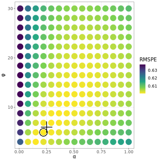
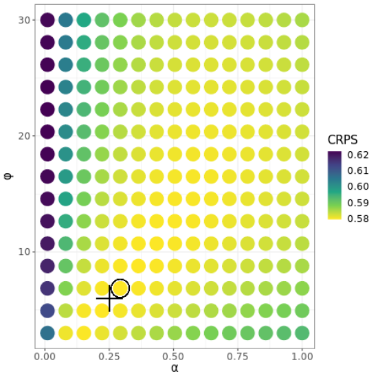
Figure 2: Simulated data analysis spConjNNGP parameter search grid and $K$-fold cross-validation results for RMSPE 2 and CRPS 2 scoring rule. The “optimal” parameter combination is circled. A plus symbol identifies the “true” $\alpha$ and $\phi$ used to generate the data.

The S3 summary method provides parameter point estimates using the optimal set and, if n.samples is specified, posterior summaries. The sub.sample argument can be used in summary if the spConjNNGP fit.rep=FALSE or if you wish for a posterior summary for a different number of n.samples. If sub.sample is specified in summary, the function returns a matrix of the requested number of samples. The output from summary(sim.c) which uses the initial number of 200 samples is given later in Table 1.

Table 1: Simulated data analysis posterior summaries of median and 95% credible interval from the three model types.

			Model type
	True	Full GP	Latent	Response	Conjugate
$\beta_{0}$	1	0.69 (0.24, 1.09)	0.62 (0.56, 0.78)	0.7 (0.27, 1.1)	0.62 (0.12, 1.19)
$\beta_{x}$	-0.1	-0.09 (-0.11, -0.07)	-0.09 (-0.11, -0.08)	-0.09 (-0.11 , -0.08)	-0.09 (-0.11, -0.08)
$\sigma^{2}$	1	0.78 (0.67, 0.98)	1 (0.85, 1.66)	0.98 (0.72, 1.32)	1.11 (1.06, 1.15)
$\phi$	6	7.58 (5.93, 9.19)	5.85 (3.57, 6.93)	5.95 (4.53, 8.16)	4.93
$\tau^{2}$	0.25	0.24 (0.23, 0.26)	0.24 (0.23, 0.26)	0.24 (0.23, 0.26)	0.25 (0.24, 0.26)

3.1.3 Model diagnostics and prediction

When passed a spNNGP or spCongNNGP object the spDiag function returns a list that, depending on the model method, includes some or all of the following elements:

• a data frame holding the Deviance information criterion (DIC) and associated values defined by Spiegelhalter et al. (2002). The DIC data frame includes rows labeled DIC the criterion (lower is better), D a goodness of fit, and pD the effective number of parameters.

• a data frame holding Watanabe-Akaike information criteria (WAIC) and associated values. The WAIC data frame includes rows labeled LPPD log pointwise predictive density, P.1 penalty term defined in unnumbered equation above Equation (11) in Gelman et al. (2013), P.2 an alternative penalty term defined in Equation (11), and the criteria WAIC.1 and WAIC.2 (lower is better) computed using P.1 and P.2, respectively.

• a data frame holding the values needed to compute the predictive criterion $D=G+P$ defined by Gelfand and Ghosh (1998). The GPD data frame includes rows labeled G a goodness of fit, P a penalty term, and D the criterion (lower is better).

• a scoring rule, see Equation 27 in Gneiting and Raftery (2007) for details, with larger values of GRS indicating better model fit.

Among the four model comparison metrics, DIC and WAIC rely on the assumption that given all the parameters (including latent ones), the data points are conditionally independent. The response and conjugate NNGP models do not preserve this conditional independence structure and do not provide samples from the latent effect. Hence, it is not appropriate to compute WAIC and DIC for them. Comparisons across the models using GPD and GRS scores require generating replicate data. We have discussed in Section 2.4 how replicates have fundamentally different interpretation for the latent and response models. For the former, the replicates are generated conditional on the latent random effects and hence are spatially correlated with the original data, whereas for the marginalized response model, the replicate is simply a new realization of a multivariate Gaussian distribution with the same mean and covariance structure as the original data. Hence, generally the GPD and GRS scores will be better for the latent models (as is evident in Table 2). It is not advisable to compare the latent and response NNGP models using GPD and GRS as they represent different principles of replication. Finally, we can compare the response model with the conjugate model using GPD and GRS as they both use the same form of replicates. However, the conjugate model uses cross-validation to tune hyper-parameters, violating the principles of all these model comparison metrics tailored for classical Bayesian procedures, and it is difficult to interpret the model comparison values for it.

The code below calls spDiag for the spNNGP latent and spConjNNGP model output sim.s and sim.c, respectively. Additionally, for comparison, we ran spNNGP for the response model (i.e., by setting method="response") and called the resulting object sim.r. Fit diagnostics for all three models are given in Table 2. However, as shown in Table 1, all models recover the “true” parameter values well, and Figure 4 shows all models produce comparable predictive surfaces.

R> s.diag <- spDiag(sim.s)
R> r.diag <- spDiag(sim.r)
R> c.diag <- spDiag(sim.c)

Table 2: Simulated data analysis output from calls to spDiag for the three model types.

		Model
	Full GP	Latent	Response	Conjugate
WAIC.1	8036.12	8034.85	–	–
WAIC.2	8501.09	8499.76	–	–
P.1	915.32	917.91	–	–
P.2	1147.8	1150.36	–	–
LPPD.2	-3102.75	-3099.52	–	–
DIC	8439.63	8438.64	–	–
pD	1318.82	1321.7	–	–
L	-2900.99	-2897.62	–	–
G	897.32	894.85	5645.59	5912.89
P	1539.07	1539.525	5234.422	6005.025
D	2436.39	2434.377	10880.01	11917.92
GRS	2975.25	2985.82	-5662.55	-5918.45

Figure 3: Observed and predicted simulated data w over the grid of holdout locations.

Given the discordance in the interpretation of the traditional model comparison metrics for the NNGP models, a pragmatic way to compare them is based on their predictive performance on a hold out set. The predict function is used to generate posterior predictive samples for new locations with associated covariates, given a spNNGP or spConjNNGP object. The code below generates posterior predictive samples for the $n_{0}$=2500 holdout locations using the latent model. The latent model is the only method that provides posterior predictive samples for the latent effect w. These samples are held in the p.w.0 matrix in the s.pred object generated below, and a summary of these samples along with the “true” w are given in Figure 3. The predict function was also called for the response sim.r and conjugate sim.c model objects to generate posterior predictive samples for the holdout locations (held in output object p.y.0) along with subsequent surface summaries in Figure 4.

R> s.pred <- predict(sim.s, X.0=cbind(1,x.ho), coords.0=coords.ho,
+   sub.sample=list(start=1000, thin=10),
+   n.omp.threads = 4, n.report=1000)

## ----------------------------------------
## ΨPrediction description
## ----------------------------------------
## NNGP Latent model fit with 5000 observations.
##
## Number of covariates 2 (including intercept if specified).
##
## Using the exponential spatial correlation model.
##
## Using 10 nearest neighbors.
##
## Number of MCMC samples 101.
##
## Predicting at 2500 locations.
##
##
## Source compiled with OpenMP support and model fit using 4 threads.
## -------------------------------------------------
## ΨΨPredicting
## -------------------------------------------------
## Location: 1000 of 2500, 40.00%
## Location: 2000 of 2500, 80.00%
## Location: 2500 of 2500, 100.00%

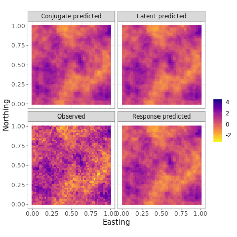
Figure 4: Observed and predicted simulated data y over the grid of holdout locations.

3.2 Timing given $n$ and number of cores

Here we provide a brief overview of the relationship between $n$, model type, and number of cores. The computer used for these runtime experiments (and analysis in subsequent sections) is running a linux operating system with a AMD Ryzen Threadripper 3990X 64-Core Processor (128 threads) and R compiled with openMP with thread-enabled MKL 2019.5.281 build with MKL_DEBUG_CPU_TYPE=5 (Intel, 2019). Timings generated by proc.time() is returned by core spNNGP functions in the run.time vector. Figure 5 provides a sense of runtime (i.e., “wall time”) needed to collect 1000 MCMC samples for $n$=100000 using the response and latent algorithms for a range of cores. Execution time for the conjugate model is about equal to one MCMC iteration of the response model. As this figure shows, for this computer and $n$, there is little speed-up beyond $\sim$40 cores mostly due to communication overhead. Then fixing the number of cores at 40, Figure 5 gives a sense of computing time required for different size $n$.

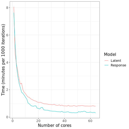
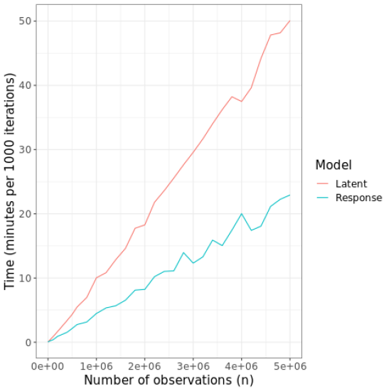
Figure 5: 5 Runtime for 1000 MCMC iterations for $n$=100000 and differnt number of cores. 5 Runtime for 1000 MCMC iterations using 40 cores and $n$ from 1000 to 5 million.

3.3 Analysis of forest canopy height

In this section we analyze a forest canopy height dataset at $n$=188,717 locations using spNNGP. Digital maps of forest structure are key inputs to many ecosystem and Earth system modeling efforts (Finney, 2004; Hurtt et al., 2004; Stratton, 2006; Lefsky, 2010; Klein et al., 2015). These and similar applications seek inference about forest canopy height variables and predictions that can be propagated through computer models of ecosystem function to yield more robust error quantification. Given the scientific and applied interest in forest structure, there is increasing demand for wall-to-wall (i.e., complete domain coverage) forest canopy height data at national and biome scales. Next generation LiDAR systems capable of large-scale mapping of forest canopy characteristics, such as ICESat-2 (Abdalati et al., 2010; ICESat-2, 2015), Global Ecosystem Dynamics Investigation LiDAR (GEDI, 2014), and NASA Goddard’s LiDAR, Hyperspectral, and Thermal (G-LiHT) Airborne Imager (Cook et al., 2013), sample forest features using LiDAR instruments in long transects or cluster designs (see, e.g., the strips of LiDAR in Figure 6). These next generation systems yield LiDAR data over the desired large spatial extents; however, the sparseness of the LiDAR sampling designs means prediction is required to deliver the desired wall-to-wall data products.

Our goal is to create high spatial resolution forest canopy height predictions, with accompanying uncertainty estimates for the Bonanza Creek Experimental Forest (BCEF; https://www.lter.uaf.edu) located in interior Alaska, USA. The BCEF domain delineated for this study, Figure 6, is $\sim$21,000 ha and includes a section of the Tanana River floodplain along the southeastern border. The BCEF is a mixture of non-forest and forest vegetation featuring white spruce, black spruce, tamarack, quaking aspen, and balsam poplar trees mixed with willow and alder shrubland species Bonanza Creek LTER (2019). Figure 6 also shows location of the $n$=188,717 G-LiHT LiDAR forest canopy height (FCH) estimates. These data are included in the spNNGP package.

The 188,717 FCH estimates come from the G-LiHT LiDAR point cloud summarized to a $13\times 13$ m grid cell size (G-LiHT: Goddard’s LiDAR, Hyperspectral & Thermal Imager, 2019). Over each grid cell, the maximum canopy height (i.e., FCH) was estimated using the 100${}^{\text{th}}$ percentile height of the point cloud. A Landsat derived percent tree cover (PTC) data product developed by Hansen et al. (2013), shown as the underlying surface in Figure 6 is used as a predictor variable for FCH. PTC is the percent tree cover estimates for peak growing season in 2010 and was created using a regression tree model applied to Landsat 7 ETM+ annual composites.

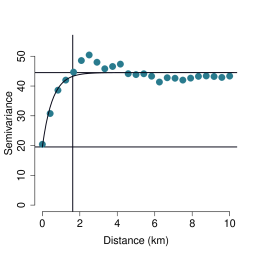
Figure 6: 6 Bonanza Creek Experimental Forest (BCEF) with G-LiHT LiDAR forest canopy height (FCH) estimates for model training and validation. The underlying map is the percent tree cover (PTC). 6 Semivariogram of BCEF non-spatial regression model residuals. Exponential covariance function estimate denoted by the curved line with associated estimates for $\tau^{2}$, $\sigma^{2}$, and the effective spatial range are given by the lower horizontal, upper horizontal, and vertical lines, respectively.

A semivariogram of the non-spatial regression model residuals can inform how the residual spatial/non-spatial variance (i.e., outcome variance not explained by the regression mean) is partitioned and the spatial range, see, e.g., Chapter 5 in Banerjee et al. (2014) for details. Here we consider the residuals from

$$\textbf{y}=\beta_{0}+\beta_{PTC}\textbf{x}+{\boldsymbol{\varepsilon}},$$ (12)

where y is the vector of observed FCH estimates, $\beta_{0}$ is an intercept, $\beta_{PTC}$ is the slope coefficient associated with the PTC predictor variable denoted as x, and ${\boldsymbol{\varepsilon}}$ is the $n\times 1$ vector following $N(\textbf{0},\tau^{2}\textbf{I}_{n})$. In the subsequent analyses we use an exponential spatial correlation function that approaches zero as the distance between locations increases. Therefore we define the distance, $d_{0}$, at which this correlation drops to 0.05 as the “effective spatial range,” which allows us to solve $\phi=-\log(0.05)/d_{0}\approx 3/d_{0}$ . Using the variog and variofit functions in the geoR package (Ribeiro Jr and Diggle, 2018), the semivarogram and empirical parameter estimates for the BCEF are given in Figure 6. Due to computational constraints we used a random subset of 25,000 residuals from (12) to generate the variogram.

3.3.1 Estimation and prediction

Here we consider the non-spatial, latent, response, and conjugate models for BCEF data. Posterior samples for the non-spatial regression model were generated using the bayesLMRef function in spBayes. Models are assessed using output from spDiag. Further, out-of-sample predictive performance was assessed by fitting the models to 100,000 observations (selected at random from the 188,717) and then predicting for the remaining holdout 88,717 observations. Finally, the models are used to predict FCH for a grid of 237,617 locations over the BCEF where PTC was recorded and resulting maps are compared.

R> n.samples <- 5000
R> starting <- list("phi"=3/2, "sigma.sq"=40, "tau.sq"=1)
R> priors <- list("phi.Unif"=c(3/10, 3/0.1), "sigma.sq.IG"=c(2, 40),
+   "tau.sq.IG"=c(2, 10))
R> cov.model <- "exponential"
R> tuning <- list("phi"=0.02)
R> bcef.s <- spNNGP(FCH~PTC, coords=c("x","y"), data=BCEF.mod,
+   starting=starting, method="latent", n.neighbors=10,
+   tuning=tuning, priors=priors, cov.model=cov.model,
+   n.samples=n.samples, n.omp.threads=40, n.report=2500,
+   fit.rep=TRUE, sub.sample=list(start=4000, thin=10))

## ----------------------------------------
## ΨBuilding the neighbor list
## ----------------------------------------
## ----------------------------------------
## Building the neighbors of neighbors list
## ----------------------------------------
## ----------------------------------------
## ΨModel description
## ----------------------------------------
## NNGP Latent model fit with 100000 observations.
##
## Number of covariates 2 (including intercept if specified).
##
## Using the exponential spatial correlation model.
##
## Using 10 nearest neighbors.
##
## Number of MCMC samples 5000.
##
## Priors and hyperpriors:
## Ψbeta flat.
## Ψsigma.sq IG hyperpriors shape=2.00000 and scale=40.00000
## Ψtau.sq IG hyperpriors shape=2.00000 and scale=10.00000
## Ψphi Unif hyperpriors a=0.30000 and b=30.00000
##
## Source compiled with OpenMP support and model fit using 40 thread(s).
## ----------------------------------------
## ΨΨSampling
## ----------------------------------------
## Sampled: 2500 of 5000, 50.00%
## Report interval Metrop. Acceptance rate: 35.12%
## Overall Metrop. Acceptance rate: 35.12%
## -------------------------------------------------
## Sampled: 5000 of 5000, 100.00%
## Report interval Metrop. Acceptance rate: 33.36%
## Overall Metrop. Acceptance rate: 34.24%
## -------------------------------------------------

For brevity, the output from subsequent calls to spNNGP for the response model and spConjNNGP are surpressed by setting verbose=FALSE.

R> tuning <- list("phi"=0.01, "sigma.sq"=0.01, "tau.sq"=0.005)
R> bcef.r <- spNNGP(FCH~PTC, coords=c("x","y"), data=BCEF.mod,
+  starting=starting, method="response", n.neighbors=10,
+   tuning=tuning, priors=priors, cov.model=cov.model,
+   n.samples=n.samples, n.omp.threads=40, n.report=2500,
+   fit.rep=TRUE, sub.sample=list(start=4000, thin=10),
+   verbose=FALSE)

R> theta.alpha <- as.matrix(expand.grid(seq(0.1,1,length.out=15),
+   seq(3/10,3/0.1,length.out=15)))
R> colnames(theta.alpha) <- c("alpha","phi")
R> bcef.c <- spConjNNGP(FCH~PTC, coords=c("x","y"), data=BCEF.mod,
+   cov.model="exponential", sigma.sq.IG=c(2, 40),
+   n.neighbors=10,
+   theta.alpha=theta.alpha,
+   k.fold = 2, score.rule = "crps",
+   fit.rep=TRUE, n.samples=200,
+   n.omp.threads=40,
+   verbose=FALSE)

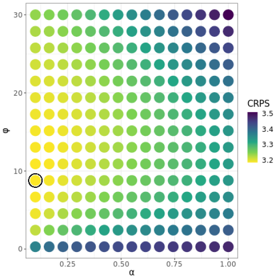
Figure 7: BCEF data analysis spConjNNGP parameter search grid and $K$-fold cross-validation results using CRPS scoring rulese. The “optimal” parameter combination is circled.

Posterior summaries are given in Table 3. As suggested by the exploratory variogram analysis, and now confirmed with formal model estimates, the spatial range is quite short, e.g., the latent model estimate of the median effective spatial range is $\sim$0.43 km (i.e., $-\log(0.05)/$6.91). Despite this short range, the spatial variance is large relative to the non-spatial variance. Such results are not surprising given the BCEF’s composition and structure are the result of myriad large and small spatial scale biotic (e.g., insect disturbance) and abiotic (e.g., soil, topography, climate, wind, fire) factors that cause spatially complex mortality and regrowth patterns. Formal model fit diagnostics provided in Table 4 suggests the addition of the latent spatial effect does improve fit compared with the non-spatial model.

Table 3: BCEF data analysis posterior summaries of median and 95% credible interval from the three model types.

	Model
	Non-Spatial	Latent	Response	Conjugate
$\beta_{0}$	1.36 (1.18, 1.49)	11.09 (10.64, 11.92)	9.94 (9.41, 10.47)	10.45 (10.07, 10.85)
$\beta_{PTC}$	0.2 (0.2, 0.2)	0.03 (0.03, 0.03)	0.03 (0.03 , 0.03)	0.03 (0.03, 0.04)
$\sigma^{2}$	–	43.48 (41.71, 45.68)	42.55 (40.6, 45.02)	34.66 (34.33, 34.89)
$\phi$	–	6.91 (6.53, 7.22)	7.19 (6.75, 7.52)	4.93
$\tau^{2}$	43.39 (43.12, 43.72)	3.46 (3.35, 3.58)	3.37 (3.27, 3.47)	3.47 (3.43, 3.49)

Table 4: BCEF data analysis model fit via spDiag and out-of-sampled prediction diagnostics for the non-spatial and three spatial model types fit to the BCEF data. The last four rows were calculated using prediction for the holdout set. The row labeled CI Cover is the percent of 95% posterior predictive distribution credible intervals that cover the observed holdout value. The row labeled CI Width is the average width of the 95% posterior predictive credible interval.

	Model type
	Non-Spatial	Latent	Response	Conjugate
WAIC.1	660845	435074.6	–	–
WAIC.2	660845	462473.1	–	–
P.1	2.35	27501.35	–	–
P.2	2.38	41200.63	–	–
LPPD.2	-330420.1	-190035.9	–	–
DIC	660845.3	464395.5	–	–
pD	2.69	56822.25	–	–
L	-330420	-175375.5	–	–
G	4387671	152329.7	7086265	6403563
P	4336921	542156.8	4119386	3502314
D	8724591	694486.5	11205651	9905877
GRS	-479230.7	-196616.3	-545860.2	-539539.6
CRPS	3.79	1.57	1.9	1.53
RMSPE	6.62	3.01	3.39	2.94
CI Cover	94.42	85.8	72.56	–
CI Width	24.73	7.82	5.76	–

Lastly, and as illustrated in the synthetic data analysis, a call to predict yields posterior predictive samples for the entire domain of interest which in this case is sampling over the grid of $n_{0}$=237617 locations where only PTC was recorded. A surface of the posterior distributions’ mean and variance are given in Figures 8 and 8, respectively. Locations where observations are available to inform prediction (i.e., along flight lines) are clearly delineated by high prediction precision in the prediction variance surfaces Figure 8. Given the relatively short spatial range this information borrowing to inform prediction does not extend too far off of the flight lines. These surfaces along with the out-of-sampled prediction performance metrics given in the last four rows in Table 4 suggest there is not too much difference among the spatial models.

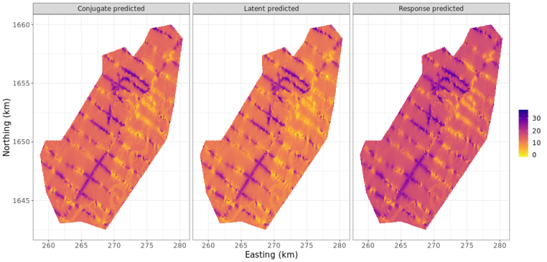
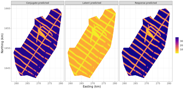
Figure 8: BCEF data analysis posterior predictive distribution mean 8 and variance 8.

3.4 Analysis of species distributions

In this Section, we present analysis of species distribution using the Binomial NNGP model. Species distribution models (SDMs) project the outcome of community assembly processes dispersal, the abiotic environment, and biotic factors onto geographic space (Guisan and Zimmermann, 2000; Pulliam, 2000). Here, we reanalyze data recently presented in Lany et al. (2020) to develop a SDM for eastern hemlock (Tsuga canadensis L.) coded as TSCA in subsequent analysis. The data comprise hemlock occurrence (Binomial outcome) on 17,743 forest stands across Michigan, USA. A set of predictors were also observed at each stand and subsequently used to explain the probability of hemlock occurrence. Predictor variables included minimum winter temperature (MIN), maximum summer temperature (MAX), total precipitation in the coldest quarter of the year (WIP), total precipitation in the warmest quarter of the year (SUP), annual actual evapotranspiration (AET) and annual climatic water deficit (DEF).

We consider three candidate models: 1) non-spatial logistic regression using the Pólya-Gamma data-augmented sampler of Polson et al. (2013) as implemented in the our spNNGP PGLogit function; 2) logistic regression with a space-varying Gaussian Predictive Process (GPP) random effect Banerjee et al. (2008) using the spBayes’ spGLM function; 3) logistic regression with space-varying NNGP again via the Pólya-Gamma sampler invoked using the family="binomial" argument in the spNNGP function as illustrated in the code below. Computational benefits of GPP models arise from the estimation of the latent Gaussian process at set of locations referred to as knots, where the number of knots is typically much smaller than $n$. When applying a GPP the analysis must strike an acceptable balance between computing time, which is governed by the number of knots, and Gaussian Process being approximated. More details about implementing a GPP can be found in Banerjee et al. (2008), Finley et al. (2009), Guhaniyogi et al. (2011), and Stein (2014). Here, for simplicity, we selected 25 knots on a fixed grid over the domain as it yielded a reasonable approximation to the desired GP with a computing time close that that of the NNGP. All three models were fit using $n$=15,000 observations and assessed using goodness of fit metrics and out-of-sampled predictive performance based on a holdout set of $n_{0}$=2,743.

Like a spNNGP class object, the return object from the PGLogit function can be passed to spDiag to yield model diagnostics as illustrated in the code below. Both PGLogit and spNNGP with faimly="binomial" accept different number of trials for each location, i.e., $n_{i}$ in Section 2.3, which is passed via the weights argument; however, for the current setting we accept the default of all weights equal to 1, i.e., each stand yields either presence or absence of hemlock.

R> n.samples <- 10000
R> starting <- list("phi"=3/50, "sigma.sq"=10)
R> tuning <- list("phi"=0.05)
R> priors <- list("phi.Unif"=c(3/300, 3/10), "sigma.sq.IG"=c(2, 10))
R> cov.model <- "exponential"
R> m.s <- spNNGP(TSCA~MIN+MAX+SUP+WIP+AET+DEF, coords=c("long","lat"),
+   data=mi.mod, family="binomial", method="latent", n.neighbors=10,
+   starting=starting, tuning=tuning, priors=priors,
+   cov.model=cov.model, n.samples=n.samples, n.report=5000,
+   fit.rep=TRUE, sub.sample=list(start=9000), n.omp.threads=40)

## ----------------------------------------
## ΨBuilding the neighbor list
## ----------------------------------------
## ----------------------------------------
## Building the neighbors of neighbors list
## ----------------------------------------
## ----------------------------------------
## ΨModel description
## ----------------------------------------
## NNGP Latent model fit with 15000 observations.
##
## Number of covariates 7 (including intercept if specified).
##
## Using the exponential spatial correlation model.
##
## Using 10 nearest neighbors.
##
## Number of MCMC samples 10000.
##
## Priors and hyperpriors:
## Ψbeta flat.
## Ψsigma.sq IG hyperpriors shape=2.00000 and scale=10.00000
## Ψphi Unif hyperpriors a=0.01000 and b=0.30000
##
## Source compiled with OpenMP support and model fit using 40 thread(s).
## ----------------------------------------
## ΨΨSampling
## ----------------------------------------
## Sampled: 5000 of 10000, 50.00%
## Report interval Metrop. Acceptance rate: 39.96%
## Overall Metrop. Acceptance rate: 39.96%
## -------------------------------------------------
## Sampled: 10000 of 10000, 100.00%
## Report interval Metrop. Acceptance rate: 39.78%
## Overall Metrop. Acceptance rate: 39.87%
## -------------------------------------------------

Parameter estimates for the three models are given in Table 5, and shows that a number of the predictor variables help explain the probability of hemlock occurrence across the study area. Due to possible spatial confounding (Hanks et al., 2015), we should interpret the sign and significance of these regression parameters in the spatial models with caution. Within sample fit diagnostics given in Table 6 and out-of-sample receiver operating characteristic (ROC) prediction curves (based on $n_{0}$=2,743 holdout locations) given in Figure 9, suggest the latent spatial variables improve the species distribution models over that of the non-spatial model. Among the spatial models, the NNGP model outperforms the reduced rank predictive process model. The computing times per 1000 samples for the non-spatial, GPP, and NNGP models are 3, 13, and 9 seconds, respectively, using 10 cores.

Table 5: Michigan Eastern Hemlock SDM analysis posterior summaries of median and 95% credible interval from the three candidate models.

	Model
	Non-Spatial	GPP 25 knots	NNGP Latent
$\beta_{0}$	-2.65 (-2.72, -2.59)	-3.6 (-3.71, -3.45)	-4.77 (-5.08, -4.47)
$\beta_{MIN}$	0.51 (0.39, 0.64)	0.74 (0.56, 0.9)	0.13 (-0.22, 0.42)
$\beta_{MAX}$	-0.21 (-0.3, -0.12)	-0.12 (-0.26, 0.01)	-0.02 (-0.36, 0.21)
$\beta_{SUP}$	0.19 (0.11, 0.27)	-0.12 (-0.23, -0.03)	-0.16 (-0.44, 0.09)
$\beta_{WIP}$	-0.01 (-0.1, 0.07)	0.12 (-0.01, 0.25)	0.01 (-0.27, 0.32)
$\beta_{AET}$	-0.41 (-0.54, -0.27)	-0.32 (-0.49, -0.16)	-0.31 (-0.52, -0.1)
$\beta_{DEF}$	-0.44 (-0.53, -0.34)	-0.35 (-0.48, -0.23)	-0.28 (-0.42, -0.13)
$\sigma^{2}$	–	4.12 (2.33, 8.46)	8.45 (6.95, 9.79)
$\phi$	–	0.01 (0.01, 0.01)	0.08 (0.06, 0.1)

Table 6: Michigan Eastern Hemlock SDM analysis model fit via spDiag and out-of-sample prediction diagnostics for the non-spatial and two spatial models.

	Model
	Non-Spatial	GPP 25 knots	NNGP Latent
WAIC.1	7494.56	6889.75	5252.05
WAIC.2	7494.6	6890.07	5511.65
P.1	6.8	27.92	623.02
P.2	6.82	28.07	752.82
LPPD.2	-3740.48	-3416.96	-2003
DIC	7494.58	6888.86	5410.72
pD	6.82	27.02	781.7

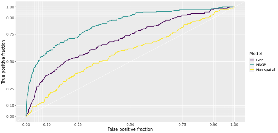
Figure 9: Michigan Eastern Hemlock SDM analysis out-of-sample posterior predictive mean ROC curves for the candidate models. Models with better prediction have curves closer to the top left corner.

3.5 Statistical gap-filling of a massive remotely sensed data

As reviewed in Section 1, methods and software are now emerging that can readily fit geostatistical models to data sets comprising locations in the 10s to 100s of thousands. However, as the number of observations climb into the millions, inferential and software options are quite limited. It is common to encounter data sets of such size in a variety of fields. For example, remotely sensed data of this magnitude either as gridded or scattered data products is now ubiquitous. Here we consider a massive-scale “gap-filling” exercise of missing Normalized Difference Vegetation Index (NDVI)—a measure of vegetation greenness— data from around 39 million locations. The NDVI data for a LandSat 8 sensor image was taken over Limpopo National Park, Mozambique, Africa on 7/17/2015. The image shown in Figure 10 has $n_{0}=$778644 pixels that are missing NDVI (denoted in gray) due to cloud cover during image acquisition. The red box in Figure 10 delineates a region with a large number of missing pixels. Filling in missing NDVI values for this and other images in a time series over Limpopo was a step in a larger study conducted by Desanker et al. (2019) that looked at environmental drivers in vegetation phonology change. Our aim is to build a geostatistical model to predict the $n_{0}$ missing NDVI pixels given the $n$=38825052 observed NDVI pixels and complete coverage land surface elevation predictor variable shown in Figure 10.

Figure 10: 10 Normalized Difference Vegetation Index (NDVI) LandSat 8 sensor image over Limpopo National Park, Mozambique, Africa on 7/17/2015, with gray pixels indicate missing NDVI data. 10 land surface elevation used to help explain variation in NDVI.

While a MCMC solution is feasible via a call to spNNGP the runtime would be on the order of days, even on a multiprocessor computer. Therefore we opt for a MCMC-free approach using spConjNNGP—trading some inference about the spatial process parameters for substantially decreased computing time. An initial variogram analysis using a sample of residuals from NDVI regressed on elevation helped define spConjNNGP’s theta.alpha search grid of 100 $\phi$ and $\alpha$ combinations, and for setting the prior for $\sigma^{2}$. As noted in the code below, we used minimum CRPS to select the optimal set of covariance parameters (i.e., specified via the score.rule argument).

R> theta.alpha <- as.matrix(expand.grid(seq(1.5, 0.01, length.out=10),
+   seq(3/200, 3/25, length.out=10)))
R> colnames(theta.alpha) <- c("alpha","phi")
R> ser.c <- spConjNNGP(ndvi~elev, coords=c("x","y"), data=ser.mod,
+   cov.model="exponential", sigma.sq.IG=c(2,0.01),
+   n.neighbors=10,
+   theta.alpha=theta.alpha,
+   k.fold = 2, score.rule = "crps",
+   X.0 = cbind(1,ser.ho$elev),
+   coords.0 = as.matrix(ser.ho[,c("x","y")]),
+   n.omp.threads=40)

## ----------------------------------------
## ΨStarting k-fold
## ----------------------------------------
##
  |
  |                              |   0%
  |
  |***************               |  50%
  |
  |******************************| 100%
## ----------------------------------------
## ΨModel description
## ----------------------------------------
## NNGP Conjugate model fit with 38825052 observations.
##
## Number of covariates 2 (including intercept if specified).
##
## Using the exponential spatial correlation model.
##
## Using 10 nearest neighbors.
##
## Source compiled with OpenMP support and model fit using 40 thread(s).
## ------------
## Priors and hyperpriors:
## Ψbeta flat.
## Ψsigma.sq IG hyperpriors shape=2.00000 and scale=0.01000
## ------------
## Predicting at 778644 locations.
## ------------
## ΨEstimation for parameter set(s)
## Set phi=0.12000 and alpha=0.01000

Given the size of this data set, the search time to identify nearest neighbor sets can take a considerable amount of time, even when using the Ra and Kim (1993) fast code book algorithm invoked by search.type="cb". In this case the search time was 8.86 minutes (search proc.time() is held in neighbor.info$nn.indx.run.time$ in the model object). Once the optimal $\phi$ and $\alpha$ was found, the runtime for parameter estimation and prediction for the missing pixels was 31.13 minutes. We have experimented with a variety of tree-based data structures (e.g., $kd$-trees modified to accommodate the nearest neighbor search constraints) and associated search algorithms, and believe there are substantial gains in search time efficiency to be had with additional development.

As shown below, a subsequent call to summary returns the optimal parameter set as well as point estimates for the other model parameters. Given the large size of this data set, parameter variance estimates are remarkably small (for some parameters the variance might be smaller than machine precision). The message at the end of the summary output reminds us that posterior samples were not requested in the initial call to spConjNNGP or summary. Generating a reasonable number of posterior samples for parameters would take a few hours for a data set of this size.

R> summary(ser.c, digits = 8)

##
## Call:
## spConjNNGP(formula = ndvi ~ elev, data = ser.mod, coords = c("x", "y"),
##     n.neighbors = 10, theta.alpha = theta.alpha, sigma.sq.IG = c(2,
##         0.01), cov.model = "exponential", k.fold = 2, score.rule = "crps",
##     X.0 = cbind(1, ser.ho$elev), coords.0 = as.matrix(ser.ho[, c("x",
##         "y")]), n.omp.threads = 40)
##
## Model class is NNGP, method conjugate, family gaussian.
##
##             Estimate   Variance
## (Intercept) 0.14544817 0.00002334
## elev        0.00155903 0.00000000
## sigma.sq    0.06520584 0.00000000
## phi         0.12000000 0.00000000
## alpha       0.01000000 0.00000000

## If posterior summaries are desired, then either rerun spConjNNGP with
fit.rep=TRUE, or specify the summary argument sub.sample to indicate the
number of fitted and replicated samples to collect.

For prediction, as illustrated in the previous analyses, we can pass the spConjNNGP object ser.c to predict. Alternatively, a slightly more efficient option (which avoids computing observed location covariance with their neighbor set twice, i.e., once for estimating parameters in spCongNNGP and again in subsequent call to predict) is to specify the prediction locations and associated design matrix via coords.0 and X.0 in the initial call to spConjNNGP. In this case, ser.c includes mean (y.0.hat) and variance (y.0.hat.var) estimates for the prediction locations. These predicted mean and variance of the mean estimates are shown for the missing pixels delineated by the red box in Figure 10 (see Figure 11 for a zoomed in view) in Figures 11 and 11, respectively. As expected, the prediction variance surface shows that pixels close to observed pixels have higher precision due to borrowing of information through the spatial correlation structure.

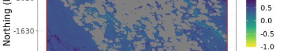
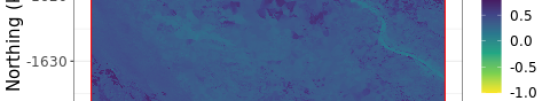
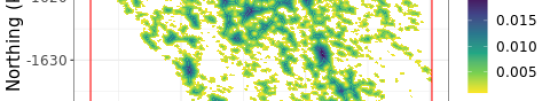
Figure 11: 11 NDVI image subset identified by the red box in Figure 10, with gray pixels indicate missing NDVI data. 11 missing pixel posterior predictive distribution mean. 11 missing pixel posterior predictive distribution variance.

4 Summary

The spNNGP R package provides a suite of NNGP-based (Datta et al., 2016) spatial regression models for both Gaussian and non-Gaussian point-referenced outcomes that are spatially indexed. The package implements the MCMC and MCMC-free algorithms detailed Finley et al. (2019) with the addition of the Pólya-Gamma latent variable model for binomial outcomes. Special care was taken to design algorithms that take advantage of multiprocessor computer via OpenMP and those with threaded BLAS and LAPACK libraries. Our future aim is to add functionality to accommodate multivariate outcomes, where we envisage two settings, first, where a limited number of outcomes (e.g., fewer than 10) might be handled using a NNGP linear model of coregionalization (Gelfand et al., 2004), second, where the number of outcomes is larger and requires some dimension reduction, e.g., via a NNGP spatial factor model, akin to the model detailed in Taylor-Rodriguez et al. (2019). For such highly multivariate data, besides factor models, we will also explore new multivariate covariance functions using sparse inter-variable graphical models that parsimoniously capture the relationship between multiple variables. Future releases will also provide the flexibility to specify a general space-varying coefficient model like the spBayes spSVC function (Finley and Banerjee, 2020). Finally, our current functions for delivering exact Bayesian inference using conjugate models for the response will be expanded to accommodate latent spatial effects (Zhang et al., 2021) and multivariate spatial regression using the matrix-variate Normal and Inverse-Wishart families.

References

- Abdalati et al. (2010) Abdalati W, Zwally H, Bindschadler R, Csatho B, Farrell S, Fricker H, Harding Dand Kwok R, Lefsky M, Markus T, Marshak A, Neumann T, Palm S, Schutz B, Smith B, Spinhirne J, Webb C (2010). “The ICESat-2 Laser Altimetry Mission.” Proceedings of the IEEE, 98(5), 735–751.
- Abdulah et al. (2018) Abdulah S, Ltaief H, Sun Y, Genton MG, Keyes DE (2018). “ExaGeoStat: A High Performance Unified Software for Geostatistics on Manycore Systems.” IEEE Transactions on Parallel and Distributed Systems, 29(12), 2771–2784. ISSN 2161-9883. 10.1109/TPDS.2018.2850749.
- Banerjee (2017) Banerjee S (2017). “High-Dimensional Bayesian Geostatistics.” Bayesian Analysis, 12, 583–614.
- Banerjee et al. (2014) Banerjee S, Carlin B, Gelfand A (2014). Hierarchical Modeling and Analysis for Spatial Data, Second Edition. Chapman & Hall/CRC Monographs on Statistics & Applied Probability. Taylor & Francis. ISBN 9781439819173. URL https://books.google.com/books?id=zNLhAwAAQBAJ.
- Banerjee et al. (2008) Banerjee S, Gelfand AE, Finley AO, Sang H (2008). “Gaussian Predictive Process Models for Large Spatial Data Sets.” Journal of the Royal Statistical Society Series B, 70(4), 825–848. 10.1111/j.1467-9868.2008.00663.x.
- Barbian and Assunção (2017) Barbian MH, Assunção RM (2017). “Spatial Subsemble Estimator for Large Geostatistical Data.” Spatial Statistics, 22, 68–88.
- Bivand (2019) Bivand R (2019). CRAN Task View: Analysis of Spatial Data. 2019-02-25, URL https://cran.r-project.org/web/views/Spatial.html.
- Bonanza Creek LTER (2019) Bonanza Creek LTER (2019). http://www.lter.uaf.edu/research/study-sites-bcef.
- Cook et al. (2013) Cook B, Corp L, Nelson R, Middleton E, Morton D, McCorkel J, Masek J, Ranson K, Ly V, Montesano P (2013). “NASA Goddard’s LiDAR, Hyperspectral and Thermal (G-LiHT) Airborne Imager.” Remote Sensing, 5(8), 4045–4066.
- Cressie and Johannesson (2008) Cressie N, Johannesson G (2008). “Fixed Rank Kriging for Very Large Spatial Data Sets.” Journal of the Royal Statistical Society B, 70, 209–226.
- Dagum and Menon (1998) Dagum L, Menon R (1998). “OpenMP: An Industry Standard API for Shared-Memory Programming.” Computational Science & Engineering, IEEE, 5(1), 46–55.
- Datta et al. (2016) Datta A, Banerjee S, Finley AO, Gelfand AE (2016). “Hierarchical Nearest-Neighbor Gaussian Process Models for Large Geostatistical Datasets.” Journal of the American Statistical Association, 111(514), 800–812. 10.1080/01621459.2015.1044091. http://dx.doi.org/10.1080/01621459.2015.1044091, URL http://dx.doi.org/10.1080/01621459.2015.1044091.
- Desanker et al. (2019) Desanker G, Dahlin KM, Finley AO (2019). “Environmental Controls on Landsat-Derived Phenoregions Across an East African Megatransect.” Ecosphere, In press.
- Emery (2009) Emery X (2009). “The kriging update equations and their application to the selection of neighboring data.” Computational Geosciences, 13(3), 269–280.
- Finley and Banerjee (2020) Finley AO, Banerjee S (2020). “Bayesian spatially varying coefficient models in the \pkgspBayes \proglangR package.” Environmental Modelling & Software, 125, 104608. ISSN 1364-8152.
- Finley et al. (2015) Finley AO, Banerjee S, Gelfand A (2015). “\pkgSpBayes for Large Univariate and Multivariate Point-Referenced Spatio-Temporal Data Models.” Journal of Statistical Software, Articles, 63(13), 1–28. ISSN 1548-7660.
- Finley et al. (2019) Finley AO, Datta A, Cook BD, Morton DC, Andersen HE, Banerjee S (2019). “Efficient Algorithms for Bayesian Nearest Neighbor Gaussian Processes.” Journal of Computational and Graphical Statistics, 28, 401–414.
- Finley et al. (2009) Finley AO, Sang H, Banerjee S, Gelfand AE (2009). “Improving the Performance of Predictive Process Modeling for Large Datasets.” Computational statistics & data analysis, 53(8), 2873–2884.
- Finney (2004) Finney MA (2004). “FARSITE: Fire Area Simulator - model development and evaluation.” Technical Report Research Paper RMRS-RP-4, U.S. Department of Agriculture, Forest Service, Rocky Mountain Research Station.
- Furrer (2016) Furrer R (2016). \pkgspam: SPArse Matrix. \proglangR package version 1.4-0, URL https://CRAN.R-project.org/package=spam.
- Furrer and Sain (2010) Furrer R, Sain SR (2010). “\pkgspam: A Sparse Matrix \proglangR Package with Emphasis on MCMC Methods for Gaussian Markov Random Fields.” J. Stat. Softw., 36(10), 1–25. URL http://www.jstatsoft.org/v36/i10/.
- G-LiHT: Goddard’s LiDAR, Hyperspectral & Thermal Imager (2019) G-LiHT: Goddard’s LiDAR, Hyperspectral & Thermal Imager (2019). https://gliht.gsfc.nasa.gov/. Accessed: 5-11-19.
- GEDI (2014) GEDI (2014). “Global Ecosystem Dynamics Investigation LiDAR.” http://science.nasa.gov/missions/gedi/. Accessed: 1-5-2015.
- Gelfand and Ghosh (1998) Gelfand AE, Ghosh SK (1998). “Model Choice: A Minimum Posterior Predictive Loss Approach.” Biometrika, 85(1), 1–11.
- Gelfand et al. (2004) Gelfand AE, Schmidt AM, Banerjee S, Sirmans CF (2004). “Nonstationary Multivariate Process Modeling Through Spatially Varying Coregionalization.” Test, 13(2), 263–312. ISSN 1863-8260.
- Gelman et al. (2013) Gelman A, Carlin J, Stern H, Dunson D, Vehtari A, Rubin D (2013). Bayesian Data Analysis, Third Edition. Chapman & Hall/CRC Texts in Statistical Science. Taylor & Francis. ISBN 9781439840955.
- Gerber (2017) Gerber F (2017). \pkggapfill: Fill Missing Values in Satellite Data. \proglangR package version 0.9.5, URL https://CRAN.R-project.org/package=gapfill.
- Gneiting and Raftery (2007) Gneiting T, Raftery AE (2007). “Strictly Proper Scoring Rules, Prediction, and Estimation.” Journal of the American Statistical Association, 102(477), 359–378.
- Gramacy (2016) Gramacy RB (2016). “\pkglaGP: Large-Scale Spatial Modeling Via Local Approximate Gaussian Processes in \proglangR.” Journal of Statistical Software, 72(1), 1–46. 10.18637/jss.v072.i01.
- Gramacy and Apley (2015) Gramacy RB, Apley DW (2015). “Local Gaussian Process Approximation for Large Computer Experiments.” Journal of Computational and Graphical Statistics, 24(2), 561–578.
- Guhaniyogi and Banerjee (2018) Guhaniyogi R, Banerjee S (2018). “Meta-Kriging: Scalable Bayesian Modeling and Inference for Massive Spatial Datasets.” Technometrics, 60(4), 430–444. 10.1080/00401706.2018.1437474.
- Guhaniyogi et al. (2011) Guhaniyogi R, Finley AO, Banerjee S, Gelfand AE (2011). “Adaptive Gaussian predictive process models for large spatial datasets.” Environmetrics, 22(8), 997–1007. 10.1002/env.1131. https://onlinelibrary.wiley.com/doi/pdf/10.1002/env.1131, URL https://onlinelibrary.wiley.com/doi/abs/10.1002/env.1131.
- Guinness (2018) Guinness J (2018). “Permutation and Grouping Methods for Sharpening Gaussian Process Approximations.” Technometrics, 60(4), 415–429.
- Guisan and Zimmermann (2000) Guisan A, Zimmermann NE (2000). “Predictive Habitat Distribution Models in Ecology.” Ecological Modelling, 135, 147 – 186. ISSN 0304-3800.
- Hanks et al. (2015) Hanks E, Schliep E, Hooten M, Hoeting J (2015). “Restricted Spatial Regression in Practice: Geostatistical Models, Confounding, and Robustness Under Model Misspecification.” Environmetrics, 26, 243–254. 10.1002/env.2331.
- Hansen et al. (2013) Hansen MC, Potapov PV, Moore R, Hancher M, Turubanova SA, Tyukavina A, Thau D, Stehman SV, Goetz SJ, Loveland TR, Kommareddy A, Egorov A, Chini L, Justice CO, Townshend JRG (2013). “High-Resolution Global Maps of 21st-Century Forest Cover Change.” Science, 342(6160), 850–853. ISSN 0036-8075. 10.1126/science.1244693.
- Heaton et al. (2019) Heaton MJ, Datta A, Finley AO, Furrer R, Guinness J, Guhaniyogi R, Gerber F, Gramacy RB, Hammerling D, Katzfuss M, et al. (2019). “A Case Study Competition Among Methods for Analyzing Large Spatial Data.” Journal of Agricultural, Biological and Environmental Statistics, 24(3), 398–425.
- Hurtt et al. (2004) Hurtt GC, Dubayah R, Drake J, Moorcroft PR, Pacala SW, Blair JB, Fearon MG (2004). “Beyond Potential Vegetation: Combining Lidar Data and a Height-Structured Model for Carbon Studies.” Ecological Applications, 14(3), 873–883.
- ICESat-2 (2015) ICESat-2 (2015). “Ice, Cloud, and Land Elevation Satellite-2.” http://icesat.gsfc.nasa.gov/. Accessed: 1-5-2015.
- Intel (2019) Intel (2019). Intel Math Kernel Library. Intel Corporation.
- Katzfuss (2017) Katzfuss M (2017). “a Multi-Resolution Approximation for Massive Spatial Datasets.” Journal of the American Statistical Association, 112(517), 201–214. 10.1080/01621459.2015.1123632.
- Klein et al. (2015) Klein T, Randin C, Korner C (2015). “Water Availability Predicts Forest Canopy Height at the Global Scale.” Ecology Letters, 18(12), 1311–1320. ISSN 1461-0248. 10.1111/ele.12525. URL http://dx.doi.org/10.1111/ele.12525.
- Lany et al. (2020) Lany NK, Zarnetske PL, Finley AO, McCullough DG (2020). “Complementary strengths of spatially-explicit and multi-species distribution models.” Ecography, 43(3), 456–466. 10.1111/ecog.04728.
- Lefsky (2010) Lefsky MA (2010). “A Global Forest Canopy Height Map from the Moderate Resolution Imaging Spectroradiometer and the Geoscience Laser Altimeter System.” Geophysical Research Letters, 37(15). ISSN 1944-8007. 10.1029/2010GL043622. L15401.
- Lindgren et al. (2011) Lindgren F, Rue H, Lindström J (2011). “An Explicit Link Between Gaussian Fields and Gaussian Markov Random Fields: The Stochastic Partial Differential Equation Approach.” Journal of the Royal Statistical Society Series B, 73(4), 423–498. 10.1111/j.1467-9868.2011.00777.x.
- Nychka et al. (2015) Nychka D, Bandyopadhyay S, Hammerling D, Lindgren F, Sain S (2015). “A Multiresolution Gaussian Process Model for the Analysis of Large Spatial Datasets.” Journal of Computational and Graphical Statistics, 24(2), 579–599.
- Plummer et al. (2006) Plummer M, Best N, Cowles K, Vines K (2006). “\pkgcoda: Convergence Diagnosis and Output Analysis for MCMC.” \proglangR News, 6(1), 7–11. URL https://journal.r-project.org/archive/.
- Polson et al. (2013) Polson NG, Scott JG, Windle J (2013). “Bayesian Inference for Logistic Models Using Pólya–Gamma Latent Variables.” Journal of the American statistical Association, 108(504), 1339–1349.
- Pulliam (2000) Pulliam H (2000). “On the Relationship Between Niche and Distribution.” Ecology Letters, 3(4), 349–361. 10.1046/j.1461-0248.2000.00143.x.
- Ra and Kim (1993) Ra S, Kim J (1993). “A Fast Mean-Distance-Ordered Partial Codebook Search Algorithm for Image Vector Quantization.” IEEE Transactions on Circuits and Systems II: Analog and Digital Signal Processing, 40(9), 576–579. 10.1109/82.257335.
- Rasmussen (2003) Rasmussen CE (2003). “Gaussian Processes in Machine Learning.” In Summer School on Machine Learning, pp. 63–71. Springer-Verlag.
- \proglangR Core Team (2018) \proglangR Core Team (2018). \proglangR: A Language and Environment for Statistical Computing. \proglangR Foundation for Statistical Computing, Vienna, Austria. URL https://www.R-project.org/.
- Ribeiro Jr and Diggle (2018) Ribeiro Jr PJ, Diggle PJ (2018). \pkggeoR: Analysis of Geostatistical Data. \proglangR package version 1.7-5.2.1, URL https://CRAN.R-project.org/package=geoR.
- Risser and Turek (2020) Risser MD, Turek D (2020). “Bayesian inference for high-dimensional nonstationary Gaussian processes.” Journal of Statistical Computation and Simulation, 90(16), 2902–2928.
- Roberts and Rosenthal (2009) Roberts GO, Rosenthal JS (2009). “Examples of Adaptive MCMC.” Journal of Computational and Graphical Statistics, 18(2), 349–367.
- Rue and Held (2005) Rue H, Held L (2005). Gaussian Markov Random Fields: Theory and Applications. Chapman & Hall/CRC Monographs on Statistics & Applied Probability. CRC Press. ISBN 9780203492024. URL https://books.google.com/books?id=TLBYs-faw-0C.
- Rue et al. (2017) Rue H, Martino S, Lindgren F, Simpson D, Riebler A, Krainski ET, Fuglstad GA (2017). \proglangINLA: Bayesian Analysis of Latent Gaussian Models Using Integrated Nested Laplace Approximations. \proglangR package version 17.06.20, URL http://r-inla.org/.
- Saha and Datta (2018a) Saha A, Datta A (2018a). “BRISC: Bootstrap for Rapid Inference on Spatial Covariances.” Stat, p. e184. 10.1002/sta4.184.
- Saha and Datta (2018b) Saha A, Datta A (2018b). \pkgBRISC: Fast Inference for Large Spatial Datasets Using BRISC. \proglangR package version 0.1.0, URL https://CRAN.R-project.org/package=BRISC.
- Sang et al. (2011) Sang H, Jun M, Huang JZ (2011). “Covariance Approximation for Large Multivariate Spatial Data Sets with an Application to Multiple Climate Model Errors.” The Annals of Applied Statistics, pp. 2519–2548.
- Spiegelhalter et al. (2002) Spiegelhalter DJ, Best NG, Carlin BP, Van Der Linde A (2002). “Bayesian Measures of Model Complexity and Fit.” Journal of the Royal Statistical Society Series B, 64(4), 583–639.
- Stein (2012) Stein ML (2012). Interpolation of Spatial Data: Some Theory for Kriging. Springer Science & Business Media.
- Stein (2014) Stein ML (2014). “Limitations on low rank approximations for covariance matrices of spatial data.” Spatial Statistics, 8, 1 – 19. ISSN 2211-6753. https://doi.org/10.1016/j.spasta.2013.06.003. Spatial Statistics Miami, URL http://www.sciencedirect.com/science/article/pii/S2211675313000390.
- Stein et al. (2004) Stein ML, Chi Z, Welty LJ (2004). “Approximating Likelihoods for Large Spatial Data Sets.” Journal of the Royal Statistical Society Series B, 66(2), 275–296. 10.1046/j.1369-7412.2003.05512.x.
- Stratton (2006) Stratton RD (2006). “Guidance on spatial wildland fire analysis: models, tools, and techniques.” Technical Report General Technical Report RMRS-GTR-183, U.S. Department of Agriculture, Forest Service, Rocky Mountain Research Station.
- Sun et al. (2011) Sun Y, Li B, Genton M (2011). “Geostatistics for Large Datasets.” In J Montero, E Porcu, M Schlather (eds.), Advances and Challenges in Space-Time Modelling of Natural Events, pp. 55–77. Berlin Heidelberg: Springer-Verlag.
- Taylor-Rodriguez et al. (2019) Taylor-Rodriguez D, Finley A, Datta A, Babcock C, Andersen H, Cook B, Morton D, Banerjee S (2019). “Spatial Factor Models for High-Dimensional and Large Spatial Data: An Application in Forest Variable Mapping.” Statistica Sinica, 29(3), 1155–1180. ISSN 1017-0405. 10.5705/ss.202018.0005.
- Vecchia (1988) Vecchia AV (1988). “Estimation and Model Identification for Continuous Spatial Processes.” Journal of the Royal Statistical Society Series B, 50, 297–312.
- Zammit-Mangion and Cressie (2017) Zammit-Mangion A, Cressie N (2017). “\pkgFRK: An \proglangR Package for Spatial and Spatio-Temporal Prediction with Large Datasets.” arXiv preprint arXiv:1705.08105.
- Zhang et al. (2021) Zhang L, Banerjee S, Finley AO (2021). “High-dimensional Multivariate Geostatistics: A Bayesian Matrix-Normal Approach.” Environmetrics, 13(3), 269–280.
- Zhang (2016) Zhang X (2016). “An Optimized BLAS Library Based on GotoBLAS2.” https://github.com/xianyi/OpenBLAS/. Accessed 2015-06-01.