A multi-wavelength study of spiral structure in galaxies. I. General characteristics in the optical

Abstract

Different spiral generation mechanisms are expected to produce different morphological and kinematic features. In this first paper in a series we carefully study the parameters of spiral structure in 155 face-on spiral galaxies, selected from the Sloan Digital Sky Survey, in the three $gri$ bands. We use a method for deriving a set of parameters of spiral structure, such as the width of the spiral arms, their fraction to the total galaxy luminosity and their colour, which have not been properly studied before. Our method is based on an analysis of a set of photometric cuts perpendicular to the direction of a spiral arm. Based on the results of our study, we compare the main three classes of spirals: grand design, multi-armed and flocculent. We conclude that: i) for the vast majority of galaxies (86%) we observe an increase of their arm width with galactocentric distance; ii) more luminous spirals in grand design galaxies exhibit smaller variations of the pitch angle with radius than less luminous grand design spirals; iii) grand design galaxies show less difference between the pitch angles of individual arms than multi-armed galaxies. Apart from these distinctive features, all three spiral classes do not differ significantly by their pitch angle, arm width, width asymmetry, and environment. Wavelength dependence is found only for the arm fraction. Therefore, observationally we find no strong difference (except for the view and number of arms) between grand design, multi-armed and flocculent spirals in the sample galaxies.

1 Introduction

Spiral arms of discoidal galaxies are remarkable structures with regions of ongoing star formation (see e.g. Calzetti et al., 2005; Elmegreen, 2011; Grosbøl & Dottori, 2012, and references therein) which are embedded into a smooth stellar disc. There are different tracers of spiral structure in galaxies (including our own Milky Way), such as Hii regions (Georgelin & Georgelin, 1976; Hou et al., 2009; Honig & Reid, 2015), OB associations (Regan & Wilson, 1993), population I Cepheids (Dambis et al., 2015; Skowron et al., 2019), giant molecular clouds (Cohen et al., 1986; Vogel et al., 1988; Wiklind et al., 1990), enhanced gas density (Grabelsky et al., 1987; Engargiola et al., 2003; Sánchez-Menguiano et al., 2017), and dust clouds (Holwerda et al., 2005).

The study of spiral galaxies is of great importance as these galaxies present a significant part (about 75% of galaxies brighter than $M_{B}=-20$) of the local Universe (Conselice, 2006). Spiral structure is thus an almost ubiquitous feature in the present disc galaxies and can also be detected in many distant galaxies up to redshift $z\sim 2$ (see e.g. Elmegreen et al., 2005; Law et al., 2012; Elmegreen, 2015). Studying the properties of spiral structure, along with other galaxy characteristics, enables astronomers to establish a theory to explain this structure and use simulations to reproduce these quantified properties and, thus, check (confirm or reject) and refine the theory proposed.

The simple classification of spirals includes three types (we will call them classes to distinguish from galaxy morphological types, see Elmegreen 1990): flocculent spiral galaxies (with many short arms, such as NGC 2841), multi-armed spirals (e.g. M 33), and grand design galaxies (with two main spiral arms, e.g. M 81). Each class, as suggested, should have its own dominant mechanism which produces the observed structure (see below).

After more than half a century of research, the physical explanation of observed spiral arms in galaxies is still debated (for a concise description of all theories, see the general review by Dobbs & Baba, 2014). There are several theories that attempt to explain spiral structure in disc galaxies. The dominant quasi-stationary density wave theory (Lin & Shu, 1964; Bertin et al., 1989a; Kalnajs, 1973; Bertin et al., 1989b) is able to successfully explain many observed properties of spiral structures. The swing amplification theory (Julian & Toomre, 1966; Gerola & Seiden, 1978; Goldreich & Tremaine, 1978; Seiden & Gerola, 1979; Toomre, 1981) implies that spiral arms are transient but recurrent structures due to local instabilities, perturbations or noise which are swing amplified into flocculent spiral arms. In the Manifold theory (Kaufmann & Contopoulos, 1996; Harsoula & Kalapotharakos, 2009; Athanassoula et al., 2009a, b, 2010; Athanassoula, 2012), spiral structure is the result of stars formed near the ends of a galactic bar moving into chaotic, highly eccentric orbits which nevertheless cause the stars to move along relatively narrow tubes called manifolds (bar driven arms). Tidal interactions were shown to produce two-armed spiral galaxies (Holmberg, 1941; Toomre, 1969; Toomre & Toomre, 1972; Elmegreen et al., 1991). Each of these mechanisms has significant support, at least for certain types of spiral galaxies. It has even been suggested that different classes (for instance, grand design versus flocculent) have different mechanisms explaining their spiral structure. It is quite likely that the mechanism differs from galaxy to galaxy and, in some cases, is represented as a combination of different models.

The overall appearance of the spiral structure may differ in different spiral galaxies proving the measurement of its parameters to be a hard task. In recent years, approaches for investigating galactic spirals have changed dramatically since observational data is now being mostly obtained via all-sky survey missions. Being a source of uniform observational data, the surveys allow for studying galactic morphology by assembling statistically significant samples.

Usually, in the literature only a few geometric parameters, which describe the spiral pattern, are considered: the number of spiral arms (Vallée, 2005; Hart et al., 2016), the pitch angle (see e.g. Kennicutt, 1981; Ma, 2002; Seigar & James, 1998; Kendall et al., 2011; Savchenko & Reshetnikov, 2013; Masters et al., 2019; Yu & Ho, 2019), and the relative amplitude of the spiral pattern (Kendall et al., 2008).

The number of arms $N_{\mathrm{arms}}$ is an important characteristic of spiral pattern which points to a possible driving mechanism of spiral structure (Hart et al., 2016; Hart et al., 2017a) and is linked to star formation (Masters et al., 2010).

The pitch angle $\psi$ is defined as the angle between the tangent of the spiral and azimuthal direction (Binney & Tremaine, 2008) and is a measure of the tightness of spiral structure. A number of properties of spiral galaxies have now been found to correlate to the pitch angle. It was found that this parameter correlates with the galaxy morphology (Kennicutt, 1981), though this trend is not as good as expected: one of the criteria for galaxy classification is the tightness of its spiral pattern (Hubble, 1936), therefore this correlation should arise automatically (see discussion in Masters et al., 2019). Other correlations, which are often discussed in the literature, are the dependence of the pitch angle on the bulge size (Freeman, 1970), the rotation properties of galaxies (Kennicutt, 1981; Seigar et al., 2005, 2006), the velocity dispersion in the central region of the galaxy (Yu & Ho, 2019), and the mass of the central supermassive black hole (Seigar et al., 2008; Davis et al., 2017). The results of these studies are often contradictory, and our understanding of spiral structure in galaxies is still incomplete.

The amplitude of spiral pattern is often expressed in terms of an amplitude of Fourier modes fitted into an azimuthal profile of a galaxy (Kendall et al., 2008; Kendall et al., 2011; Yu et al., 2018), or using direct measurements of maximal and minimal flux values along an azimuthal profile (Elmegreen et al., 2011). This parameter is found to be a good estimator of the galaxy type: galaxies of later Elmegreen classes (Elmegreen & Elmegreen, 1987, see Sect. 2.4) tend to have a spiral structure with a larger amplitude. Also, more massive galaxies harbour more prominent spirals (Kendall et al., 2015).

Another parameter, which defines a spiral arm and is hard to determine, is its width $w$. The width, in contrast to the multiple studies on pitch angle, had not been paid much attention to until recently. It has been investigated by Reid et al. (2014) for the Milky Way and by Honig & Reid (2015) for M 51, M 74, NGC 1232, and NGC 3184, using trigonometric parallaxes of masers and positions of Hii regions, respectively. In both works it has been shown that the width increases with distance from the galactic center. A similar behaviour was noted by Lynds (1970) for the width of dust lanes in spirals of ten nearby galaxies. Forgan et al. (2018) describe a method, which identifies spirals in hydrodynamic simulations of discs, and allows one to measure the widths of individual arms.

So far, the width for a statistically significant sample of appropriate (observed face-on and large enough to explore) spiral galaxies has not been investigated. As such, a detailed study of the overall spiral structure, described by the above listed parameters, appears lacking in the literature.

This is the first paper in a series where we perform a detailed study of spiral pattern for a relatively large sample of spiral galaxies by utilising observational data from modern sky surveys in a broad wavelength range from the ultraviolet (UV) to far-infrared (FIR). We aim to systematically study the properties of the spiral structure (pitch angle, arm width, number of arms, class of spiral structure, etc.), their relation to the general galaxy quantities, as well as structural composition, in dependence on wavelength. This will allow us to study, for the first time, the multi-band photometry of spiral galaxies by taking into account their main structural components (bulge, disc, bar) and asymmetric spiral pattern, and, most importantly, their interplay. The results of this study should point to possible different mechanisms which are responsible for the observed spiral pattern in galaxies.

In this first study, we investigate in the optical the general properties of spiral structure in galaxies: the pitch angle and its variation with radius, the width of the spirals and its dependence on radius, their contrast in comparison with the overall disc component (what is the fraction of the spiral structure to the total galaxy luminosity in the optical?), and colours of the spiral arms. Also, the dependence of these parameters on the general galaxy properties is investigated. To accomplish this study, we use a rather straightforward method for measuring the mentioned quantities of spiral structure and apply it to a relatively large sample of spiral galaxies.

The paper is organised as follows. We outline the sample selection, data preparation, and general properties of the sample in Sect. 2. The method, developed to derive parameters of spiral structure, is described in Sect. 3. In Sect. 4, we provide results of our analysis and discuss them in Sect. 5. We summarise our main conclusions in Sect. 6.

2 The data

In this section we describe a selection process of spiral galaxies to be analysed in our work. Also, we present details on image preparation for the selected galaxies. We classify their spiral pattern and briefly comment on the general properties of the selected sample.

2.1 Selection of the sample

To create a sample of face-on spiral galaxies whose angular size would be large enough for the purposes of this study, we make use of the following projects, based on the Sloan Digital Sky Survey (SDSS, York et al., 2000). First, from the GalaxyZoo sample (Lintott et al., 2008), we selected objects which fulfil the following criteria based on the fraction of user votes: P_CW $\geq 0.9$ (clockwise spirals) OR P_ACW $\geq 0.9$ (anticlockwise spiral) AND P_EL $\leq 0.1$ (non-elliptical galaxies) AND P_EDGE $\leq 0.1$ (non-edge-on galaxies). This query yielded 19102 galaxies, the vast majority of which are too tiny for the purposes of this paper. Therefore, all selected galaxies were processed via the HyperLeda database (Makarov et al., 2014) to identify their names and photometric parameters. From this preliminary sample, we chose galaxies with an optical diameter (calculated from the $logd25$ value from HyperLeda, as the diameter at the isophote 25 mag arcsec^-2 in the $B$ band) larger than 50″. The choice of a 50$\arcsec$ diameter is arbitrary – it was chosen to be large enough to provide a statistically significant number of galaxies of all types and, at the same time, provide a sufficient resolution for measuring the width of the spiral arms in galaxies: as we show in Sect. 4.3, a galaxy with an optical diameter of 50$\arcsec$ has, on average, an arm width of $3.5\arcsec$, which is 2.7 times larger than the average FWHM $\approx 1.3\arcsec$ of the point spread function (PSF) in the SDSS $r$ band (see Sect. 2.2). However, taking into account that the arm width is usually growing outwards from the center (see Sect. 4.3), it may have a somewhat smaller width at the beginning of the arm. Therefore, to make sure that the image resolution is sufficient for measuring the arm width at virtually all radii, we selected galaxies with HyperLeda diameters larger than $50\arcsec$. This yielded 1611 galaxies in total.

After that, we additionally revisited the EFIGI (Baillard et al., 2011) catalogue searching for large (nearby) spiral galaxies using the following criteria: $1\leq T\leq 8$ AND Arm_Strength $\geq 0.25$ AND Arm_Curvature $\geq 0.5$ AND diam $>50\arcsec$ AND ax_ratio $<1.3$. This added another 376 objects to our preliminary sample. The joined sample was examined by eye 3 times to remove highly inclined galaxies, galaxies contaminated by foreground stars, overlapping galaxies, or strongly interacting galaxies. Also, in our final sample we selected only those galaxies for which at least one spiral arm can be traced (i.e. the spiral pattern is not too flocculent, not wound up in a ring and not too weak to be analysed by our method, see Sect. 3.2). Finally, we settled on a sample of 155 (85 galaxies are found in the EFIGI sample) spiral galaxies which are appropriate for a further analysis (we should note, however, that we started with an initial sample of approximately 200 galaxies, but some of them were then removed because their spiral arms were too faint or hard to be analysed or classified). The final sample is listed in Table 1, along with some general parameters which are described in Sect. 2.4 and 2.3.

The sample suffers from some obvious selection effects which we discuss in detail in Sect. 5.

2.2 Data preparation

For our photometric analysis of galaxies, we use imaging from the SDSS DR13 (Albareti et al., 2017) in the three photometric bands $g$, $r$, and $i$. The corrected frames in each band were retrieved from the SDSS Science Archive Server (SAS) using a specially developed Python script. The mosaics out of several SDSS fields (if a galaxy covers more than one field) were prepared using the SWARP code (Bertin et al., 2002). Also, all frames were converted from NMgy back to original ADU, in order to use the signal-to-noise, the CCD gain, and the initially subtracted sky value $I_{\mathrm{sky,ini}}$ (which can be found in the supplementary SDSS tables) in our further fitting.

Although the downloaded frames have been bias subtracted, flat-fielded, and sky-subtracted, we re-estimated the sky background around each galaxy using an initial mask of all detected objects in each frame provided by sextractor (Bertin & Arnouts, 1996). The unmasked area was fitted with a 2nd polynomial (with the average value $I_{\mathrm{sky,re}}$) and subtracted from the original frame. The final sky-subtracted value is thus $I_{\mathrm{sky}}=I_{\mathrm{sky,ini}}+I_{\mathrm{sky,re}}$, with the standard deviation $\sigma_{\mathrm{sky}}$. Also, we cut out the original image: the final galaxy image should encompass the isophote at the $2\sigma_{\mathrm{sky}}$ level enlarged by a factor of 1.5. The initial mask of contaminating objects was revisited by eye to mask objects which had not been detected by sextractor or were masked erroneously.

To create a PSF image for each galaxy frame, we used the PSFEX package (Bertin, 2011), which searches for isolated non-saturated field stars near the target galaxy to compute a combined PSF image. As a rule, there were 10–20 such PSF stars, which allowed us to reliably determine an average PSF FWHM and to estimate its dispersion $\sigma_{\mathrm{FWHM}}$. The average values of the FWHM for each band are: $1.41\pm 0.16\arcsec$ (the $g$ band), $1.35\pm 0.16\arcsec$ (the $r$ band), and $1.33\pm 0.14\arcsec$ (the $i$ band).

For applying our fitting method of spiral structure, which we describe in detail in Sect. 3, we should correct the images for the projection effect. This is also important for the classification of the spiral arms (see Sect. 2.4). Galaxy discs may have an arbitrary orientation in space, which is described by the inclination $\mathfrak{i}$ and position $\mathrm{PA}$ angles. To correct an image for the projection effect, it is necessary to rotate it by a value of $\mathrm{PA}$, so that the major axis of the disc orients along the $x$-axis of the image, and then stretch the image along the $y$-axis by the value of the major-to-minor axes ratio $1/q$ of the best-fit elliptical isophote. To derive the values $q$ and $\mathrm{PA}$ (as well as some other general galaxy parameters, see Sect. 2.3), we used an iterative isophote fitting procedure (Jedrzejewski, 1987). Since the shape of the isophotes of spiral galaxies can be influenced by non-axisymmetric inner components, such as bars or spirals, it is preferable to use the outermost isophotes for our de-projection analysis. In this work, we use median values of $q$ and $\mathrm{PA}$ for ten isophotes equally spaced between the 24-th and 25-th isophotes in the $i$ band (in this band the impact of the spiral pattern on the parameters of the outermost isophotes is minimal among the $g$, $r$ and $i$ bands under consideration). We denote this median value of $q$ as $q_{25}$.

2.3 General properties of the sample galaxies

Our sample includes nearby spiral galaxies, such as PGC 5974 (M 74), and rather distant galaxies, up to $D=290$ Mpc for PGC 53625 ($z=0.067$). The mean distance for the sample is $90.0\pm 57.7$ Mpc. In Fig. 1 we show the distribution of the sample galaxies by the optical radius $r_{25}$ in the $r$ band (leftmost panel), which we estimated using the isophote fitting (see Sect. 2.2). As one can see, most galaxies have a radius less than 1.5′(the mean value $\langle r_{25}\rangle=1.2\pm 1.0\arcmin$).

The selected galaxies are mostly viewed face-on (the mean apparent flattening derived in Sect. 2.2 $\langle q_{25}\rangle=0.82\pm 0.13$), so only minor de-projection to the true face-on orientation was needed.

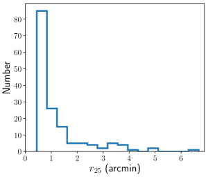
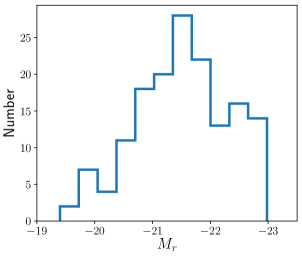
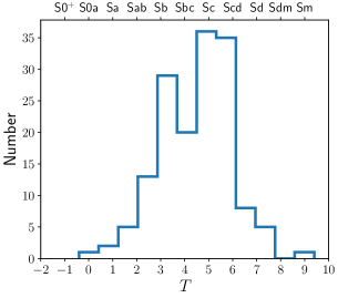
Figure 1: Distribution of the sample galaxies as a function of optical radius (leftmost panel), luminosity (middle panel), and numerical (Hubble) type (rightmost panel).

To estimate the total magnitude $m$, we created a growth curve for each galaxy image based on our isophote fitting results. Asymptotic magnitudes in each band were estimated by extrapolating the dependence of the gradient $\mathrm{d}m/\mathrm{d}r$ on magnitude $m$ to $\mathrm{d}m/\mathrm{d}r=0$ (by definition, this gives the asymptotic magnitude of the galaxy, see e.g. Muñoz-Mateos et al. 2015). From the total magnitudes we computed the absolute magnitudes in each waveband and colours $g-r$ and $r-i$, each corrected for the Galactic extinction (Schlafly & Finkbeiner, 2011) taken from the NASA/IPAC Extragalactic Database (NED). The distribution of the sample galaxies as a function of luminosity is shown in the middle panel of Fig. 1. The absolute magnitude of our sample ranges from -19 to -23 in the $r$ band, with the average $-21.5\pm 0.8$ — in our sample we consider regular spiral galaxies with a typical luminosity (see e.g. de Lapparent et al., 2011).

The right panel of Fig. 1 shows the distribution of our sample galaxies by the numerical Hubble type according to the HyperLeda database. As one can see, most numerous galaxies in our sample are of types Sb–Sc ($\langle T\rangle=3.8\pm 1.6$), with some fraction of lenticular galaxies with a faint yet detectable spiral structure and a few Sa galaxies with tightly wound spiral arms. According to the visual inspection of the galaxy images, in our sample we have 60 unbarred galaxies versus 95 galaxies with a bar.

Numerical simulations show (for example, Salo & Laurikainen 2000, Dobbs et al. 2010) that tidal interactions can be related to the formation of spiral structure in disc galaxies. In order to investigate a possible relation between the properties of spiral structure and the spatial environment of their hosts, we collected information on the spatial environment of galaxies from the NED database (specified as hierarchy) and from Tempel et al. (2012). All galaxies, which belong to a pair, a triple, a galaxy group or cluster, we classify as non-isolated, the rest galaxies – as isolated. In total, our sample comprises 45 isolated galaxies and 110 non-isolated galaxies.

Table 1: General characteristics of the sample galaxies. This table is published in its entirety in the electronic version of the MNRAS.

Name	$D$	Scale	$r_{25}$	$q_{25}$	$m_{r}$	$M_{r}$	$(g-r)_{0}$	$(r-i)_{0}$	$T$	Env	Bar
	(Mpc)	(kpc/arcsec)	(arcmin)		(mag)	(mag)	(mag)	(mag)
(1)	(2)	(3)	(4)	(5)	(6)	(7)	(8)	(9)	(10)	(11)	(12)
PGC303	73.5	0.344	1.01	0.59	13.13	-20.91	0.51	0.27	3.1	g	—
PGC2182	84.3	0.394	0.93	0.67	13.02	-21.42	0.60	0.36	4.1	p	+
PGC2440	84.3	0.394	0.57	0.81	13.51	-20.91	0.49	0.33	3.2	p?	—
PGC2600	64.6	0.304	1.01	0.88	12.02	-21.76	0.50	0.14	5.2	i	—
PGC2901	68.9	0.324	1.87	0.89	11.12	-22.78	0.73	0.46	1.6	g	+
…	…	…	…	…	…	…	…	…	…	…	…

Columns:

(1) PGC name from HyperLeda,

(2), (3) distance and scale calculated from the best distance modulus from HyperLeda,

(4) the semi-major axis of the isophote 25 mag arcsec^-2 in the $r$ band,

(5) median flattening between the 24-25 mag arcsec^-2 isophotes in the $r$ band,

(6) and (7) apparent asymptotic and absolute magnitudes in the $r$ band calculated from the growth curve, corrected for the Milky Way extinction (Schlafly & Finkbeiner, 2011),

(8) and (9) colours calculated from the corresponding asymptotic magnitudes and corrected for the Milky Way extinction (Schlafly & Finkbeiner, 2011),

(10) numerical morphological type from HyperLeda,

(11) environment: G or g – belongs to a group, P or p – belongs to a pair, T or t – belongs to a triple, I or i – isolated galaxy; C or c – belongs to a cluster. Capital and small letter mean that the information is taken from NED or Tempel et al. (2012), respectively. ‘?’ after the letter means that classification is found neither in NED nor in Tempel et al. (2012) and we classified the galaxy environment on our own using the SDSS SkyServer Navigate tool on the basis of visual closeness to the target galaxy and known spectroscopic redshift.

(12) Bar presence according to the visual inspection.

2.4 Classification of spiral structure

Galaxies can be very different in their morphological properties and thus are usually classified according to one or another schema. Since we investigate spiral arms, it is natural to use their features as a basis for our classification. The most well-known classification system for this purpose was introduced in Elmegreen & Elmegreen (1987) and represents 10 classes (AC1-AC12, AC10 and AC11 are no longer in use). However, these classes can also be combined in three main classes (Elmegreen et al., 2011; Karapetyan et al., 2018): flocculent (‘F’, Arm Classes AC1-AC3), multiple arm galaxies (‘M’, Arm Classes A4C-AC9), and grand design galaxies (‘G’, Arm Classes AC12).

Only 11 galaxies in our sample are found in the sample of Elmegreen & Elmegreen (1987) and few in Sánchez-Menguiano et al. (2017) and Karapetyan et al. (2018), where galaxies were already classified. Also, our sample includes 29 common galaxies with the S⁴G survey (Sheth et al., 2010; Buta et al., 2015). As the number of sample galaxies with available arm classes is low, we decided to classify all of them ourselves using a major voting schema between all authors of this study, similar to that used in Sánchez-Menguiano et al. (2017) and Karapetyan et al. (2018). For the voting evaluation, we used the images prepared in Sect. 2.2. We decided to use a combined approach with the 3 major classes, since our sample is not that big and the usage of the original Elmegreen & Elmegreen (1987) classification will lead to a situation, when most of the classes will be underpopulated. Each author of this paper independently assigned one of the F, M, G classes to the galaxy spiral pattern, based on the de-projected images and using the following criteria. Flocculent (F) galaxies demonstrate spiral arms which are chaotic, fragmented, asymmetric or uniformly distributed around the centre. Grand design (G) galaxies have two distinct long symmetric arms dominating the disc. The remaining multiple arm (M) class includes the following situations: the galaxy exhibits only one prominent arm (the others are flocculent), more than two prominent continuous arms, or two symmetric arms in the inner part and multiple irregular outer arms (plums), or vice versa. We consider the classification of a galaxy to be reliable if at least three votes have the same class.

For the 155 galaxies from the initial sample at least three authors voted for the same class and for approximately half of them all four authors were unanimous in their classification. Galaxies with unreliable classification mostly demonstrate transition between F and M classes and were removed from the initial sample of around 200 galaxies, see Sect. 2.1. The final sample comprises of 20 F, 100 M and 35 G galaxies.

It is difficult to directly compare our classification results to other works, since our sample is obviously biased to galaxies with distinct spiral pattern and thus should not represent any unbiased distribution. In Sánchez-Menguiano et al. (2017), the authors studied a sample of spiral galaxies in the SDSS $g+u$ bands. They used two classes and reported 45 galaxies classified as flocculent and 18 as grand design galaxies. Our classification holds near the same ratio if we consider M-class galaxies closer to flocculent. In Buta et al. (2015), a classification is given for 1114 S⁴G spiral galaxies in the $3.6\mu$ m band, based on the same classification scheme as we use. From these galaxies, 29 are common with our sample. For half of them, Buta et al. (2015) listed the same class as we assign, but for the other 13 galaxies, their class is different. However, in all cases the reported classes are close i.e. G vs M or M vs F (the second combination is more often). This comparison supports, in some way, our classification, besides the fact that the sample in Buta et al. (2015) is more biased to the F class (50% F, 32% M, and 18% G cases, but the ratio G:M+F is again close to ours) and besides the fact that some galaxies can demonstrate a very different view of the spiral pattern at different wavelengths (the S⁴G survey is a near-infrared survey, whereas here we consider the $gri$ bands). For example, NGC 5055 and NGC 2841 can be classified as F in the optical and G in the near-infrared (Thornley, 1996).

We should stress here that the flocculent galaxies in our sample have better-defined spiral arms because of the described in Sect. 2.1 selection criteria than usually analysed in the literature. Therefore, our category of flocculent galaxies does not map one-to-one onto those used by other authors.

In Fig. 2 we show nine typical spiral galaxies in our sample of the G, M and F classes.

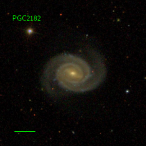
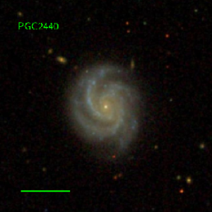
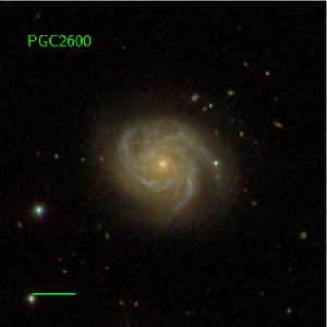
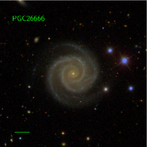
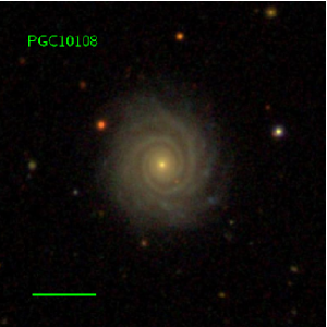
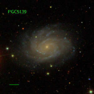
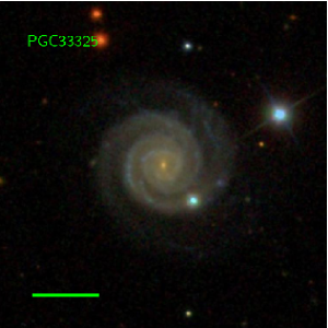
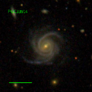
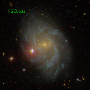
Figure 2: SDSS thumbnail images for nine typical spiral galaxies in our sample: left column are of G-class (PGC2182, PGC26666, PGC33325), middle column – M-class (PGC2440, PGC10108, PGC33914), and the right one shows F-class spirals (PGC2600, PGC5139, PGC8631). A bar in the bottom left corner of each image shows one arcminute scale. The images are oriented such that the north direction is up and the west is right.

Along with the arm classification, we counted the number of well-distinct spiral arms (though not all of them can be analysed with our method because of their faintness or visible bifurcations, see Sect. 3) as an indirect test of the classification correctness. If the number of spiral arms is larger than 5 or cannot not be counted (for flocculent galaxies), we assign to this number ‘>5’. Fig. 3 demonstrates the distribution of grand design, multi-armed and flocculent galaxies of our sample by the number of spiral arms. One can see, that all grand design galaxies in our sample have a two-armed spiral structure, whereas multi-armed and flocculent galaxies may have different number of spiral arms, from 2 to >5. Flocculent galaxies tend to have, on average, a larger number of spirals than multi-armed galaxies.

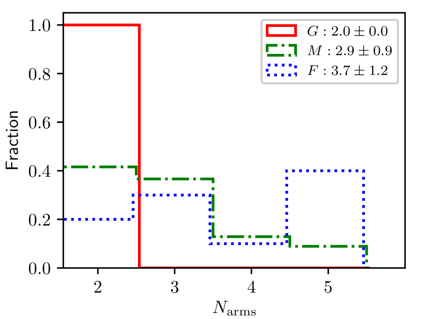
Figure 3: Distribution of grand design (red solid line), multi-armed (green dash-dotted line) and flocculent (blue dotted line) galaxies in our sample by the number of spiral arms.

3 The method

In this section we outline our method for analysing spiral structure in galaxies. We start with some additional image preparation which is required for our method to work. Then we describe the method itself. At the end of this section, we illustrate the results of the method applied to a galaxy from our sample.

3.1 Additional image reduction

One additional step of the image preparation has not yet been done – removing an axisymmetric component from the galaxy image. The spiral arms are observed as an additional component over the stellar disc, the light from which can interfere with the spiral arms when their parameters are measured. To remove the light of the disc from the galaxy image, we subtracted an azimuthal profile of the galaxy from the original image. To compute the profile, we found the mean flux value along a set of concentric ellipses of different sizes with the ellipticity fixed to $\cos\mathfrak{i}$ and position angle to $\mathrm{PA}$ of the galaxy (see Sect. 3.1). To suppress small scale flux variations, we applied an iterative sigma clipping procedure before the averaging. Our azimuthal profile is axially symmetric, so by subtracting it we remove an axially symmetric component (the disc) from the image and leave in the image only non-axially symmetric components, such as spirals, a bar, star-forming regions etc.

After this additional step, the galaxy images are ready to be processed with our analysis.

3.2 Method outline

The main idea of our method is to analyse a set of photometric cuts made across spiral arms at various points of the spiral structure. The local parameters of a spiral arm (such as the width of the arm at a given point) are derived from the properties of the corresponding slice, whereas the global parameters (such as the pitch angle and the overall width variation along the arm) can be inferred from the analysis of the whole set of such slices. The slices should cover the entire arm, from the beginning to the end with some given step.

It is proven to be extremely difficult (see e.g. Davis & Hayes, 2014) to determine automatically if a given point of an image belongs to a spiral structure, and to group such points into separate spirals: local kinks, discontinuities, forks, and background objects lead to splitting the arms or to joining separate arms together. In this work we decided to visually inspect each galaxy image and manually put some points along the spiral arms to use them as a first-guess tracer of the spiral arm for our method. To do so, we used the DS9 package to display a de-projected galaxy image and place several circular regions along each prominent spiral arm. The radii of these regions were adjusted such that the regions spanned approximately to the middle of the interarm area covering the full width of the arm. The radii of the regions were used to calculate the lengths of the slices. If an arm is splitting into two arms at some point, we chose the brightest branch (which also usually follows the general direction of the parent arm). If an arm is splitting into two arms of roughly the same amplitude, or has more than one splitting point, we discard it.

In the next step, the algorithm fills in gaps between the sparse user-specified points to trace the whole spiral arm, with a step of 2 pixels. For every pair of adjacent points $i$ and $j$, a local value of the pitch angle is estimated as

$$\psi_{ij}=\operatorname{atan}\left(\frac{\log r_{j}-\log r_{i}}{\phi_{j}-\phi_{i}}\right)\,,$$

where $r$ and $\phi$ – are polar coordinates of the points. The space between these two points is then filled using an interpolation by a logarithmic spiral with a constant value of the pitch angle:

$$r_{k}=r_{i}\exp\left(\tan\psi\left(\phi_{i}-\phi_{k}\right)\right)\,,$$

where values of $\phi_{k}$ are evenly spaced between $\phi_{i}$ and $\phi_{j}$ such that the new points are located at a distance of about 2 pixels from each other.

After that the algorithm makes photometric cuts perpendicular to the arm at every point. The slope of a line perpendicular to a logarithmic spiral with the pitch angle $\psi$ at the point with azimuth $\phi$ can be found as

$$\xi=-\frac{\tan\psi\cos\cos\phi-\sin\phi}{\tan\psi\sin\phi+\cos\phi}\,.$$

To enhance the signal-to-noise ratio, we make several cuts placed with a small shifts along the arm and then compute an averaged cut using a median filter. This averaging also allows us to filter out small-scale flux variations, such as compact Hii regions and unmasked stars: the flux variation across the cut is higher in such regions, so the corresponding pixels can be assigned with smaller weights during the subsequent analysis. At this stage we also use the mask of the background objects (see Sect. 2.2) to exclude the masked pixels. Fig. 4 demonstrates schematically the construction of a cut.

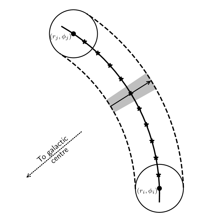
Figure 4: A scheme of an orthogonal cut construction. The curved solid line depicts a spiral arm, with two circles to be user specified points $i$ and $j$ (see text). The stars show locations of the interpolated points at which the cuts are made. One of the cuts is shown as a solid line with an arrow with a shaded region to be the cut width. The dashed lines show the limits of the cuts.

When a photometric cut is made at a given point of an arm, we fit it with an analytical function. Schematically, a cut across a spiral arm should appear as a bell-shaped curve with a peak located near the centerline of the spiral and gradually decreasing brightness at both sides of the peak (Fig. 5).

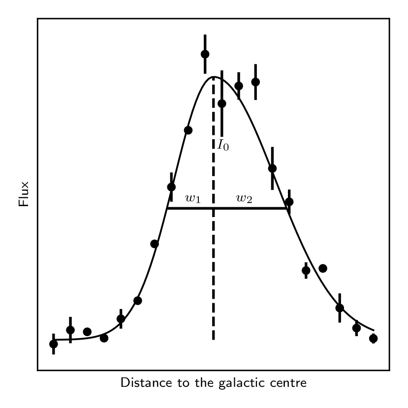
Figure 5: A schematic view for a single slice. The dots are data points, the solid line is a fit by a lopsided Gaussian. The peak location is shown by the vertical dashed line and the amplitude and both widths are marked as $I_{0}$, $w_{1}$ and $w_{2}$. The errorbars show the flux variation across the cut.

To fit such a bell-shaped curve and also to take into account possible asymmetry of a spiral arm, we adopted an asymmetric Gaussian function as a fitting function:

$$I_{\mathrm{model}}(r)=I_{0}\times\begin{cases}\exp\left(-\frac{\left[r-r_{\mathrm{peak}}\right]^{2}}{w_{1}^{2}}\right),&r<r_{\mathrm{peak}}\\ \exp\left(-\frac{\left[r-r_{\mathrm{peak}}\right]^{2}}{w_{2}^{2}}\right),&r>r_{\mathrm{peak}}\,,\end{cases}$$ (1)

where $I_{0}$ is the amplitude, $r_{\mathrm{peak}}$ is the peak location, and $w_{1}$ and $w_{2}$ are the half-widths of the spiral arm “inward” (in the direction to the galactic centre) and “outward” (away from the centre), accordingly. When $w_{1}=w_{2}$, the brightness distribution is symmetric around the peak at this point of the arm. If $w_{1}<w_{2}$, the inner side of the arm is steeper than the outer one (as in Fig. 5), and vice versa. We also added a free baseline level to the fitting function as a linear trend. The fitting function has, therefore, six free parameters ($I_{0}$, $r_{peak}$, $w_{1}$, $w_{2}$ and two parameters for a baseline level).

Since the observed image of a galaxy is a real image convolved with a point spread function, a direct measurement of the parameters of the spiral structure via the fitting procedure will yield distorted values (a lower amplitude and larger widths). To solve this problem, one should convolve the fitting function with the PSF before comparing it with the observed flux inside the fitting procedure. Therefore, the real fitting function has to be written as:

$$I_{\mathrm{fitting}}=I_{\mathrm{model}}*\mathrm{PSF}\,,$$

and the fitting parameters should be inferred from this function. If the derived value of the FWHM of the (unconvolved) cut is lower than the PSF FWHM, the spiral at this point is too thin to be resolved in the image, and the corresponding width value should be considered as unreliable and has to be excluded from the further analysis. Another reason for discarding a slice from the analysis is a low signal-to-noise ratio. If the measured amplitude $I_{0}$ is lower than the background variation, we also consider this slice as unreliable. The outermost slice of each spiral arm is, therefore, the last slice with the amplitude above the background variation level. We consider a slice with the amplitude equal to the background variation level as still reliable because the slice is constructed as a mean of $\sim 10$ adjacent slices, so the effective noise variation for it is lower, and the outermost slices are detected at the $\sim 3\sigma$ level.

To estimate the uncertainties of the fitting parameters within a slice, we run a Monte-Carlo simulation. We repeated our fitting process of a cut many times randomising the flux values of the cut points according to their uncertainties. The errors of the fitting parameters are then estimated as standard deviations of their values within these randomised runs.

3.3 The output values

Here we describe the parameters of the spiral structure which are derived by means of our algorithm for an example galaxy, PGC 2182 (Fig. 2, left panel). The results of the application of the algorithm to the entire sample are shown in Sect. 4.

As a main output of the algorithm at every point of the galactic spiral structure, we derive:

• coordinates of the peak position,

• surface brightness of the spiral arm at this point,

• characteristic values of spiral widths, “inward” and “outward”.

Fig. 6 illustrates results of our fitting process applied to PGC 2182 and plotted over the image, which was created as a residual between the de-projected galaxy image and azimuthally averaged model in the $r$ band. The white circles show locations of the positions of the cut peaks, computed from the $r_{\mathrm{peak}}$ values; the solid lines show inner and outer edges of the arms computed from $w_{1}$ and $w_{2}$ values, correspondingly. We use a Savitzky-Golay filter to smooth the locations of both peak positions and arm edges before plotting them since they are influenced by the overall flocculence of the spiral structure on small scales whereas we are interested in large scale variations of the arm parameters. The letters A and B mark spirals for further references.

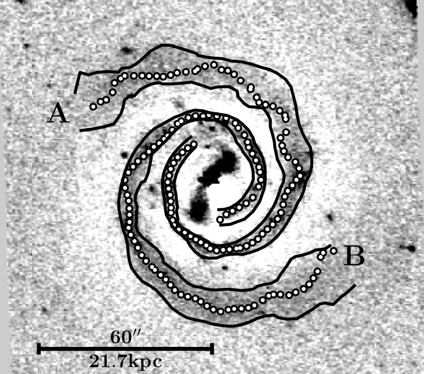
Figure 6: Results of the fitting of the spiral arms for PGC 2182 in the $r$ band. The white points show locations of the cut peaks, the solid lines show inward and outward widths of spirals. The line in the bottom left corner shows a 60″scale for the image (which is 21.7 kpc at the distance to the galaxy).

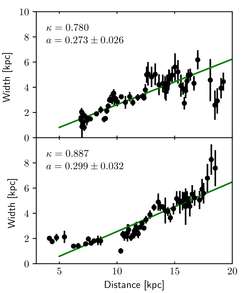
Figure 7: Values of the full width of the spirals A (top) and B (bottom) for PGC 2182 as a function of radius. In top left corners of each panel, the values of the Pearson coefficient $\kappa$ and the slope of the best-fit linear fit are shown. The fit itself is shown as a green solid line. The gaps in the data are due to the exclusion of the unresolved slices (see text).

One can see from Fig. 6 that the width of the spirals changes with radius. Fig. 7 demonstrates this in a form of width–radius relations: the top panel shows the full width ($w=w_{1}+w_{2}$) of the arm A as a function of radius, the same relation for the arm B is shown in the bottom panel. One can see that in the case of PGC 2182, the widths of both arms systematically increase with the distance from the galaxy centre. The values of $\kappa$ in top left corners of each panel show a Pearson correlation coefficient for these width – radius relations, and the values of $a$ are slopes of best linear fits (i.e. average rates of the width change with radius in kpc per kpc).

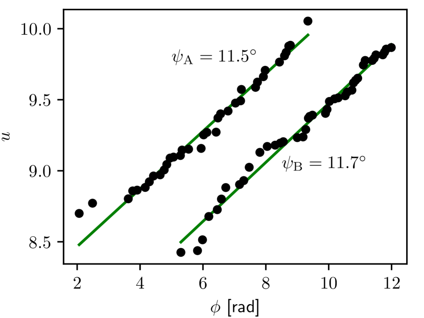
Figure 8: Pitch angle estimation for the two arms of PGC 2182: the points show the spiral arms in the log-polar coordinate system, and the green solid lines are the best linear fits to the data.

Having values of $w_{1}$ and $w_{2}$ for each point of the spiral structure, we can compute some measure of the asymmetry of the spiral arm. In this work, we decided to compute the asymmetry as

$$A=\frac{w_{2}-w_{1}}{w_{2}}\,.$$ (2)

Positive values of $A$ mean that the inner side of an arm has a steeper slope then the outer one (as on Fig. 5).

Another value that can be derived from our analysis is a pitch angle value. If a spiral arm can be described by a logarithmic spiral, it will appear as a straight line in the log-polar coordinates. The slope of this line is determined by the pitch angle value of the arm:

$$u=u_{0}+\tan\psi\cdot\phi\,,$$

where $u=\log r$ and $u_{0}=\log u_{0}$. The pitch angle, therefore, can be found as a slope of a linear fit of the points of the spiral structure in the log-polar coordinates (Kennicutt, 1981; Font et al., 2019). Fig. 8 demonstrates the pitch angle determination for PGC 2182. The solid lines show linear fits to the data, and the value of the pitch angle is shown for both spirals. The advantage of this approach is that the value of the pitch angle can be derived individually for all spirals of the galaxy, in contrast to the widely used Fourier analysis applied to a galaxy image (Considere & Athanassoula, 1982), which yields only some average value for the entire spiral structure.

Our further analysis of the pitch angle includes an investigation of the pitch angle variation with radius. To compute local values of the pitch angle at different galactocentric distances, we used a spatial window. This window isolates a part of the arm located at a given range of the radii, so that the pitch angle inference can be applied only for this part of the arm. Moving the window along the arm, one can measure how the pitch angle changes with distance to the galaxy centre. In this work, we use a window width equal to one-third of the full arm extent. This window size allows one to capture a general trend of the pitch angle variation while still having a high signal-to-noise ratio.

Since our method yields the values of the pitch angle for all spiral arms separately, it is possible to estimate the value of the interarm pitch variation $\frac{\Delta\psi_{\mathrm{arms}}}{\left<\psi\right>}$, i.e. the value that shows the variation of the pitch angle value between the galaxy spirals. We define this value as a difference between the maximal and minimal pitch angles for all arms divided by the mean value of the pitch angle for the galaxy (so $\frac{\Delta\psi_{\mathrm{arms}}}{\left<\psi\right>}=0$ indicates that all spirals in the galaxy have the same value of the pitch angle).

Using the peak positions and width values, it is possible to construct an image which contains the spiral mask. This spiral mask is an image of the same size as the original galaxy image and has pixel values equal to 1 if the corresponding pixel belongs to the spiral structure (i.e. it lies between the solid lines in Fig. 6), and 0 otherwise.

The constructed spiral masks can be used in several ways. At first, we use them to rectify azimuthal profile subtraction (Sect. 3.1). The problem is that when we compute an azimuthal profile, the spirals also contribute to it, even if a sigma clipping procedure is applied. This leads to an overestimation of the disc brightness which, in its turn, leads to negative intensities in the interarm regions of the residual image (the result can be seen in Fig. 6 for PGC 2182: the interarm regions are brighter than the background regions which surround the galaxy and have the zero mean flux). This effect does not alter the results related to the positions and scales (the peak positions, widths, pitch angles), but can introduce a systematic shift in the results related to the brightness (spiral arm colours and fluxes).

To fix this problem, we performed azimuthal averaging once again, but with the additional mask of the spiral arms this time. When the spirals are masked out, they do not make a contribution to the azimuthal profile, so the true disc background can be computed and subtracted from the galaxy image. This, however, can be achieved only when a galaxy has a regular spiral pattern and all the spirals can be reasonably covered by a mask. Some galaxies in our sample (mostly of the classes M and F) have splitting spirals (bifurcations) or contain fragments of spirals, so their masks do not cover the entire spiral structure. We therefore selected a subsample of galaxies with a regular spiral structure and performed a further analysis which requires a proper azimuthal subtraction only for this subsample. Hereafter, we call this subsample as “stage 2” galaxies, to stress that the analysis of the spiral structure was applied two times for them: the first time – with a default azimuthal profile and the second time – with a profile, for creating of which a mask of all spiral arms was taken into account. In total, our sample contains 67 of such stage 2 galaxies, which include 29 grand design spirals, 33 multi-armed and 5 flocculent galaxies.

Once the azimuthal profile is corrected for the presence of the spiral structure, the “original minus model” residual image should mainly contain the light coming from non-axisymmetric galaxy components. We then use the spiral mask to isolate the spirals and compute a total flux coming from the spiral pattern of the galaxy. This flux value can be then used to compute the arms-to-total ratio $f_{\mathrm{arms}}$ by dividing it by the total aperture flux of the galaxy. This presents a new method for the “arms strength” estimation, completely independent of existing techniques such as $m=2,3,4$ Fourier modes strength (for example, Kendall et al. 2011, Yu et al. 2018). Comparing the spiral flux in different passbands, we can also compute a colour of the spiral structure.

The radial brightness profile of a spiral is another property of the spiral structure which can be obtained using our algorithm. Having a set of points along the arm, one can find how the arm surface brightness changes with radius. Fig. 9 shows the radial surface brightness distribution for the two spiral arms of PGC 2182. The spirals of this galaxy show approximately exponential radial brightness profiles. An exponential scale of this profile can be derived via a linear fit of the data. The solid line in Fig. 9 shows results of a linear fit and the values in the top right panels are the derived values of the exponential scale. This arm exponential scale length will be discussed in a future work, where we are about to perform a photometric decomposition of our sample galaxies and study the dependence between different structural parameters and spiral structure.

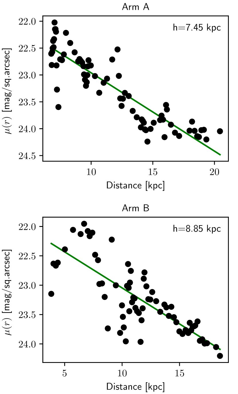
Figure 9: Surface brightness distribution (computed from the fitted $I_{0}$)

for the spirals of PGC 2182 as a function of radius. The solid line in each panel is a linear fit of the corresponding surface brightness distribution. The derived values of the exponential scale are shown in top right corners of each panel.

4 Results

In this section we present the results of our analysis applied to the whole sample of the selected galaxies. In Table 2, we list the main fitting and other important parameters of the spiral structure for the entire sample. In this section we only consider results for the $r$ waveband, as this band is the deepest among the other SDSS bands and we have checked that the results in the other bands are similar to what we derived for this band (see Sect. 5.3).

Table 2: Results of the fitting for the $r$ band. This table is published in its entirety in the electronic version of the MNRAS.

Name	$\langle\psi\rangle$	$\frac{\delta\psi}{\langle\psi\rangle}$	$w$	$a$	$A$	$f_{\mathrm{arms}}$	$(g-r)_{\mathrm{arms}}$	$T_{\mathrm{arms}}$	$N_{\mathrm{arms}}$
	(deg)		($r_{25}$)
(1)	(2)	(3)	(4)	(5)	(6)	(7)	(8)	(9)	(10)
PGC303	23.0	0.4	0.13	-0.007	0.27	0.15	0.44	M	4
PGC2182	11.5	0.2	0.14	0.286	0.12	0.25	0.46	G	2
PGC2440	17.2	—	0.14	0.108	-0.17	—	0.50	M	3
PGC2600	23.9	0.3	0.10	0.179	0.02	0.13	0.27	F	3
PGC2901	9.1	1.0	0.10	0.153	0.21	0.13	0.58	G	2
…	…	…	…	…	…	…	…	…

Columns:

(1) PGC name from HyperLEDA,

(2) mean pitch angle averaged for all spiral arms we traced,

(3) relative pitch angle variation along the radius,

(4) mean width of spiral arms (in units of $r_{25}$) averaged for all spiral arms we traced,

(5) slope of the best linear fit to the radial width variation (positive values mean that the width increases with radius),

(6) mean asymmetry of the cuts (positive values mean that the inner slope of the cuts is steeper),

(7) fraction of the spiral pattern in the total galaxy flux in the $r$ band,

(8) $(g-r)$ colour of the spiral pattern,

(9) armclass: G – grand design, M – multi-armed, F – flocculent,

(10) total number of arms we counted for each galaxy.

4.1 Reliability of the results

In this section we test the reliability of the obtained results in several possible ways. To do so, we validate some characteristics we measured in this study, such as the pitch angles, disc inclinations, total magnitudes, compared to those from other available sources. In addition to that, we discuss individual slices of our fitting, uncertainties obtained from Monte-Carlo simulations and do an indirect comparison of the arm widths derived from other works and known techniques for extracting information on the spiral arms. It is important to mention here that two tests have been already done: the quality of our classification was evaluated in Sect. 2.4 and all measured arm widths are greater than the corresponding PSF FWHM by design (see Sect. 3.2): 23% of all slices were removed from the analysis due to insufficient resolution (most of them are in the inner regions of the galaxies).

To verify that our galaxy de-projection is correct, we compared the apparent disc flattening $q_{25}$, estimated in Sect. 2.2, with that given in the HyperLeda database as $logr25$ (measured in the $B$ band) and converted to the the minor-to-major axis ratio. We found that these parameters correlate well with the Pearson correlation coefficient $\kappa=0.69$, the slope 1.02 and the zero-intercept. Therefore, we can be assured that our de-projection is reliable.

In order to validate our photometry data, we find an intersection with the Catalog Archive Server (CAS) database from the SDSS DR13. For 146 galaxies in this intersection, we compared our total magnitudes from Table 1 to the Petrosian magnitude petroMag from the SDSS database. Besides the fact that these magnitudes are not equally comparable, the coincidence between the two magnitudes is good with a small number of exceptions (PGC 38240, PGC 51592, and PGC 43161). For two of these exceptions, the reason for this discrepancy can be an erroneous galaxy center location in the CAS database. After removing the outliers, the average Pearson correlation coefficient for all three bands equals 0.97. In all cases, the values of the Petrosian magnitude are slightly larger as compared to our measurements, which means that galaxy is fainter and which is natural according to the definition of the Petrosian magnitude. The average difference in the magnitudes for all galaxies is around 0.5 in the $g$ band and 0.3 in the $r$ and $i$ bands.

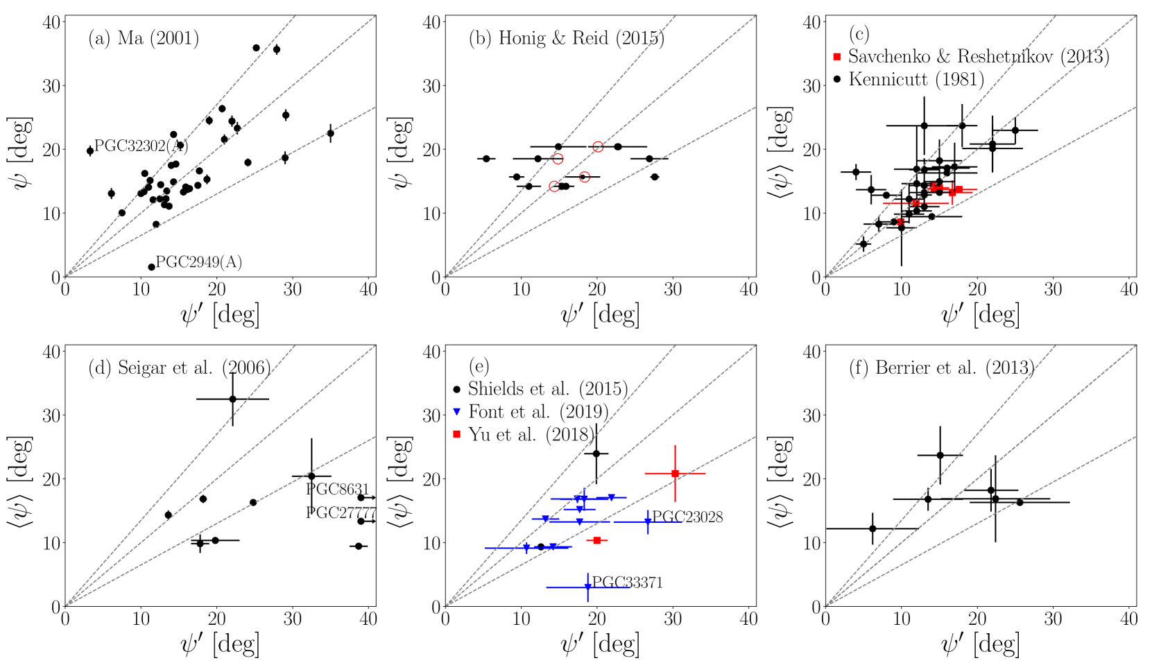
Figure 10: Comparison of the pitch angles found in this work with other sources. The dashed lines show a diagonal and 30%-margin error. The pitch angles are shown for the $r$ band. For galaxies from the other works with a single pitch angle found, we plot $\langle\psi\rangle$ (see Table 2) and show the scatter between different arms as the uncertainty bar. The sources used are (a) Ma (2001); (b) individual arcs from Honig & Reid (2015), the circles represent an average value between the arcs for one arm; (c) Savchenko & Reshetnikov (2013) in $g$ band (red squares) and Kennicutt (1981) (black circles); (d) Seigar et al. (2006) for the $B$ band, arrows show two galaxies with both $\psi^{\prime}$ and uncertainties $>40\degr$; (e) Shields et al. (2015) (black circles) in the $g$ (PGC24531) and $B$ band (PGC2600), Font et al. (2019) (blue triangles), Yu et al. (2018) (red squares) in the $R$ band for 2DFFT; (f) Berrier et al. (2013).

The pitch angle of spiral structure has been measured for a significant number of galaxies in different works. For common galaxies, we compare our measures with those derived in these works (denoted as $\psi^{\prime}$). The result of this comparison is presented in Fig. 10. The comparison in almost all cases is indirect because we find angles separately for each spiral arm detected, while in most other works only one angle is measured for the whole pattern, usually according to some Fourier-based technique. Only in Ma (2001) the pitch angles were determined for each arm separately and can be compared directly.

We have 26 galaxies in intersection with Ma (2001), from which 12 galaxies have only one common spiral arm measured and 14 galaxies – two spiral arms. The upper left subplot (a) in Fig. 10 shows a good agreement between all values except two cases, which can be a result of the different de-projection method used in Ma (2001). In Honig & Reid (2015), the authors carried out a detailed analysis of H ii regions for four galaxies, in which they measured pitch angles for individual arcs in an arm. Two of these galaxies, M 74 (PGC 5974) and NGC 3184 (PGC 30087), are included in our analysis, both with two spiral arms measured. The comparison in subplot (b) in Fig. 10 demonstrates that individual parts of the arms can differ from our measured $\psi$, but their average value is close to it. As the remaining (c) – (f) subplots show, in all other cases the agreement is good and the errors are within a 30% margin, even besides the variety of methods used for the pitch angle estimation, whether it is by fitting a line to the $\phi$ vs $\log r$ data, or using one-dimensional Fast Fourier Transforms (1DFFT) and two-dimensional Fast Fourier Transforms (2DFFT), or by the so-called spirality method (Shields et al., 2015). One exception is shown in the subplot (d) with a severe disagreement with the values taken from Seigar et al. (2006). However, it has been recently reported that the pitch angles, determined in Seigar et al. (2006), can have a significant discrepancy with other works (see, for example, fig. 8 and 9 and related discussion in Yu & Ho, 2019). Finally, in subplot (e), the pitch angle found in Font et al. (2019) for PGC 33371 is much larger than we measure here, which can be an effect of different parts of the spiral arm used for estimating its pitch angle (the same is true for PGC 23028, but with a lower significance). In total, we compared our pitch angles with the literature for 48 galaxies, and the comparison demonstrates a good agreement with the other works.

As to the width of spiral structure, there are few works with measured widths and in all cases only several individual objects were studied (Foyle et al., 2010; Puerari et al., 2014; Honig & Reid, 2015), so it is impossible to compare our results with these sources due to a lack of common objects.

To estimate the goodness of the slices fitting procedure, we find reduced $\chi^{2}$ statistic for all individual slices. The mean value for $\chi^{2}$ does not differ much between the $gri$ bands and varies from 1.13 in the $i$ band to 1.07 in the $r$ band. These values, which are close to unity, indicate that the match between the observations and estimates is in accord with the error variance. Thus, we can conclude that, on average, the usage of an asymmetric Gaussian function leads to a good, non-overfitted representation for the slices.

As mentioned in Sect. 3.2, we run a Monte-Carlo simulation with 25 realisations in order to validate the global stability of the procedure used and to estimate uncertainties on the derived output values. We find that all three $gri$ bands show similar results in these simulations. The coordinates of the peak position show both average and median uncertainty around 10% of the slice length. The surface brightness of the spiral arm at this point varies even less than that. The standard deviations of the “inward” and “outward” spiral widths increase and are slightly less than 20%, on average. These uncertainties become bigger for faint parts of the arm, which are usually located in the external regions of the galaxy. However, estimating the arms-to-total ratio for a spiral mask of an individual Monte-Carlo realisation gives an uncertainty of just several percent. For the pitch angle $\psi$ and slope $a$, the uncertainty between the realisations is less than the difference between the individual arms. In total, our simulations demonstrate good stability for the obtained results and that all findings we present in the next sections should be valid if we take into consideration the uncertainties from these Monte-Carlo simulations.

Finally, it is interesting to compare results, which were obtained with automated arm-detection techniques, to our approach. Foyle et al. (2010) and Davis & Hayes (2014) developed such methods which should be compared with in this paper. Davis & Hayes (2014) apply a sophisticated computer vision algorithm called SpArcFiRe, which detects arm segments and extracts structural information about a spiral arm (the code is publicly available). We attempted to apply this code to our galaxy images, but the output results are always covered by many detected arcs (see also a note on this in Yu et al. 2018), which obviously do not belong to the spiral pattern. A possible reason for that is a need in additional image processing or more proper tuning various parameters of their algorithm which, unfortunately, cannot be done by the unprepared user. Another method, which was developed in Foyle et al. (2010), is based on a Fourier transform where arms are detected as all pixels above some threshold in a reconstructed image. Unfortunately, it has been shown that besides discarding asymmetric features and including emission features as part of the arms themselves, the strongest mode in DFFT does not always fit the spiral pattern (see discussion in Yu et al. 2018) and, thus, cannot be reliable. The detailed comparison with other 1DFFT and 2DFFT methods, which can only detect an arm itself but not its boundaries, is beyond the scope of this paper.

4.2 Pitch angle

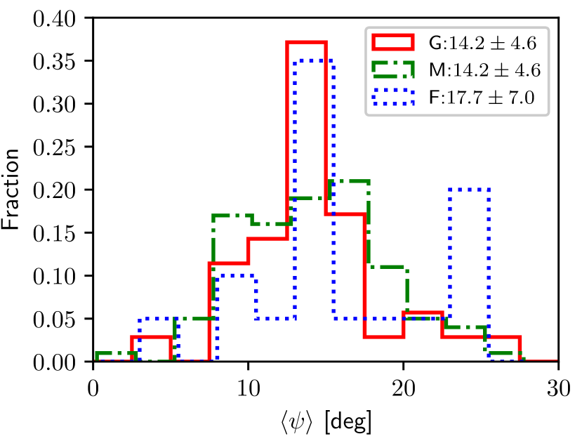
Figure 11: Distribution of grand design (red solid line), multi-armed (green dash-dotted line) and flocculent (blue dotted line) galaxies by the pitch angle value.

Fig. 11 shows the distribution of galaxies of different arm classes by the mean pitch angle value $\langle\psi\rangle$, averaged for all arms we traced in our analysis. The mean value of the pitch angle for all sample galaxies is $14.8\pm 5.3$°  which is close to those found in the literature (see e.g. Kennicutt, 1981; Ma, 2001; Savchenko & Reshetnikov, 2013). Galaxies of all three spiral arm classes demonstrate peaks around 15° , although we notice a second peak around 25°  for flocculent galaxies. In general, we do not see a statistically significant difference between the distributions by the pitch angle for the different arm classes. This result is in line with Puerari & Dottori (1992), who found that there is no correlation between the pitch angle and arm class. However, Hart et al. (2017b) studied a large stellar mass-complete sample of spiral galaxies and concluded that multi-armed spirals are looser (by 2° ) than two-armed spirals. A similar conclusion can be made from the results by Díaz-García et al. (2019), based on the imaging for spiral galaxies from the S⁴G survey (see their table 2 and fig. 12): grand design spirals have lower pitch angles (by several degrees) than flocculent and multi-armed ones. Though we do not see this difference for our much smaller sample, the average difference in winding of several degrees between the different arm classes is rather small and definitely lies within the standard deviation for each class (see the legend in Fig. 11) and within the uncertainty of pitch angle estimation. In this and other studies we can clearly see that grand design and multi-armed spirals may almost equally have very small or vice versa very large pitch angles. Therefore, the pitch angle is definitely not a good characteristic to discriminate between different arm classes, and, potentially, arm generation mechanisms.

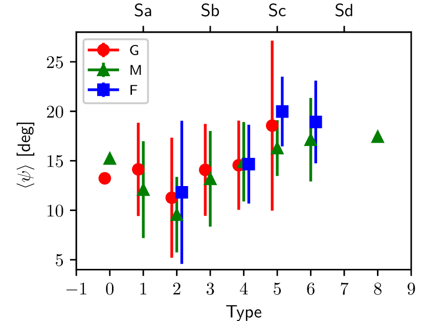
Figure 12: Mean pitch angle values as a function of morphological type.

Fig. 12 shows the mean values of the pitch angle as a function of Hubble type. Although there is a weak general trend of increasing pitch angle with Hubble stage, the overall dispersion is quite large such that each type has a significant overlapping in the measured pitch angles with other types. Here again we cannot see a difference between the arm classes within a bin of morphological stage.

We collected estimates of the pitch angle from different sources (most representative samples were used). We show the correlation between the pitch angle and morphological type in Fig. 13 (the sources are listed in the caption to the Figure). As one can see, the correlation is very weak for almost all samples. Yet, the trend is still visible: early-type spirals (Sa) are, on average, most tightly wound, whereas late-type spirals (Sd) have a tendency to be open; intermediate spirals may have various pitch angles. It is fair to note here that the results from Kennicutt (1981) show a better correlation as compared to the other results. We selected common galaxies in each pair from the sources used and found that the results of Kennicutt (1981) are significantly different from the other sources. If we exclude the Kennicutt’s sample from the consideration, the average difference in the pitch angles between the remaining sources is $13\pm 14.6$% of the average pitch angle calculated for these sources; if we compare the Kennictutt’s sample alone with the other sources (by pairs), this turns out to be $-19\pm 51$%, with many early-type spirals having a too small pitch angle as compared to the other sources, see Fig. 13, the left bottom corner. The reason for this discrepancy is not clear and, probably, is hidden in the method used for measuring the pitch angle in Kennicutt (1981). Also, the weak and scattered trend between the pitch angle and morphology may signify that the modern morphological classification of spiral galaxies is more related to the bulge prominence rather than to the spiral structure (see the discussion in Masters et al. 2019).

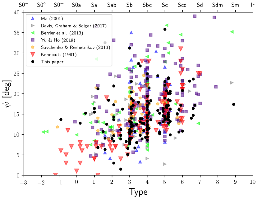
Figure 13: Correlation between the pitch angle and Hubble stage for different results taken from the literature: Ma (2001), Davis et al. (2017), Berrier et al. (2013), Yu & Ho (2019), Savchenko & Reshetnikov (2013), Kennicutt (1981), and this work.

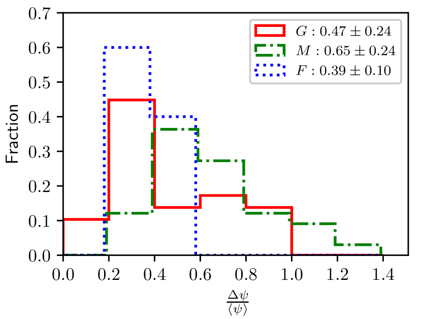
Figure 14: Distribution of the pitch angle variations for grand design (red solid line), multi-armed (green dash-dotted line) and flocculent (blue dotted line) classes.

Fig. 14 shows the distribution of the sample galaxies based on the relative pitch angle variation defined as a standard deviation of all pitch angle values along the spiral arm divided by the mean value of the pitch angle. Again, this is an average value for all arms under study. Only stage 2 galaxies (galaxies with the full coverage of their spiral structure, see Sect. 3.3) were included in this Figure (the measurement of the relative pitch variation made by a part of the spiral arm would give a lower value). This distribution confirms the findings by Savchenko & Reshetnikov (2013) and Díaz-García et al. (2019) that most galaxies demonstrate significant pitch angle variations: the average value of the relative pitch angle variation is $0.56\pm 0.25$, which means that the pitch angle value may vary by more than 50% along the radius. Grand design galaxies show somewhat lower pitch angle variations ($0.47\pm 0.24$) than galaxies with multi-armed spirals ($0.65\pm 0.24$). The number of flocculent galaxies of stage 2 (only 5 galaxies) is insufficient for making a firm conclusion on the pitch angle variations for these spirals, though the selected flocculent spirals do not demonstrate such large variations as multi-armed galaxies. However, according to the results from Díaz-García et al. (2019), flocculent galaxies also show slightly smaller variations of the pitch angle than grand design and multi-armed galaxies ($\sigma(\psi)=7.9\pm 5.4\degr$ versus $8.6\pm 4.6\degr$ and $10.1\pm 4.0\degr$, respectively).

In total for the sample, we find that the dispersion of the pitch angle along the radius is $\sigma(\psi)=7.2\pm 3.3\degr$ which is slightly less than found in Díaz-García et al. (2019) ($\sigma(\psi)=9.2\pm 5.0\degr$, where they measured the standard deviation of the pitch angle of different spiral segments) for galaxies at 3.6 $\mu$m. However, similar to Díaz-García et al. (2019), we also find that the differences of the pitch angle along the radius for individual galaxies can be $>15-17\degr$.

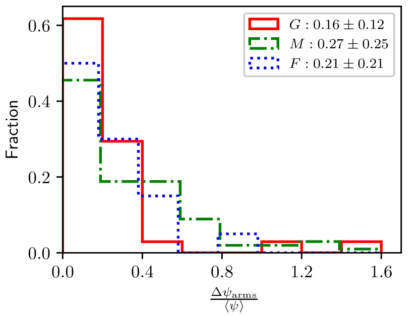
Figure 15: Distribution of the sample galaxies by the pitch angle variations between the arms. Grand design, multi-armed and flocculent galaxies are shown in red (solid line), green (dash-dotted line) and blue (dotted line) colours, respectively.

Fig. 15 shows the distribution of the galaxies from our sample by the relative difference between the average pitch angles for individual arms (divided by the average pitch angle for all spiral arms) $\frac{\Delta\psi_{\mathrm{arms}}}{\left<\psi\right>}$. One can see that for all arm-classes the distribution looks similar: galaxies tend to have arms with close pitch angle values (the difference between the pitch angles for different arms is, on average, about 20-25% of their mean value). However, there are also galaxies for which $\frac{\Delta\psi_{\mathrm{arms}}}{\left<\psi\right>}$ may differ up to 100%. The mean value of the pitch angle variation between the arms for grand design galaxies is somewhat smaller than for multi-armed ones ($0.16\pm 0.12$ and $0.27\pm 0.25$, respectively), i.e. the spirals in grand design galaxies tend to have closer values of the pitch angle than in galaxies with multi-armed spiral pattern.

4.3 Width of spiral arms

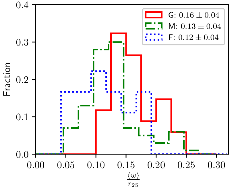
Figure 16: Distribution by average spiral width expressed in units of the optical radius $r_{25}$ for grand design (solid red line), multi-armed (green dash-dotted line) and flocculent galaxies (blue dotted line).

Fig. 16 shows the distribution of galaxies by the mean value of the width of spiral structure. It is calculated as a mean value of the full width $w=w_{1}+w_{2}$ at every point on the spiral structure and is represented here in units of the optical radius in the $r$ band (see Sect. 2.2). The mean value of the width for the sample is $(0.14\pm 0.05)\,r_{25}$. If we express the arm width in kpc, for grand design spirals $w=3.3\pm 1.2$ kpc, $2.5\pm 0.9$ kpc for multi-armed and $2.1\pm 1.4$ kpc for flocculent galaxies. Both quantities of $w$ show that grand design spirals have a slightly larger width, whereas flocculent galaxies have the narrowest spirals and multi-armed galaxies lie in between.

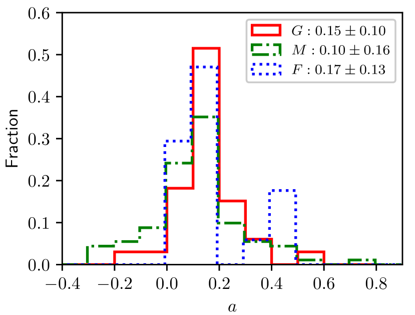
Figure 17: Distribution by the slope for the radius – spiral width relation in the $r$ band.

Fig. 17 shows the distribution of the galaxies by the slope $a$ for the dependence between the galactocentric radius and spiral width (see Sect. 3.3 and Fig. 7), where we can see how the arm width changes with radius. One can see that most galaxies in our sample (85.8%) demonstrate a positive slope which means that the width of their spiral arms increases with galactocentric distance. This result is in agreement with Honig & Reid (2015) where for four galaxies it was shown that the width of all their major arms increases with radius. However, in our sample we can also find galaxies with the spirals arms, which have a nearly constant width, and also galaxies with the arms becoming thinner at the periphery. For example, PGC 49881 ($a=-0.18$) has quite abrupt and unusual spirals which indeed do not look wider in the outer galaxy region. The multi-armed spiral galaxy PGC 48478 ($a=-0.30$) also shows thinner spiral arms when going outwards. By contrast, PGC 49401 exhibits much wider spiral arms ($a=0.78$) at large radii than in the inner region. If we compare the distributions by this parameter for different arm classes, we can see that multi-armed galaxies have slightly lower average values of $a$ than grand design galaxies. However, statistically this difference is not significant.

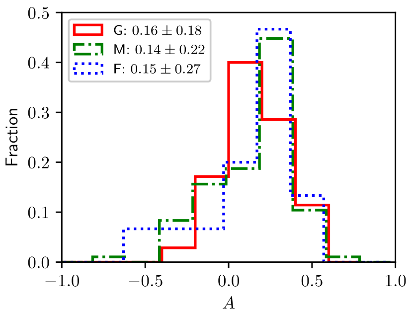
Figure 18: Distribution of the sample galaxies by the asymmetry values in the $r$ band.

Fig. 18 shows the distribution of the sample galaxies by the value of the mean asymmetry of the slices perpendicular to the spiral arms (see eq. 2). The mean asymmetry is computed as an average value for each slice for all spirals in a galaxy. Most galaxies (75.3%) in our sample have a positive asymmetry value, which means that the inner side of their arms $w_{1}$ is narrower, on average, than the outer side $w_{2}$. The average value of the asymmetry $0.14\pm 0.23$ means the $w_{2}$ half-width is approximately 16% larger than the $w_{1}$ half-width. Numerical simulations predict (Yuan & Grosbol, 1981) that for the density-wave scenario this should be the case: inside of the co-rotation radius, the shock is formed behind the spiral arm, and, therefore, we can expect that $w_{2}$ should be larger than $w_{1}$. Interestingly, all three spiral classes do not show any difference in the distributions by the width asymmetry.

4.4 Luminosity and colour of spiral structure

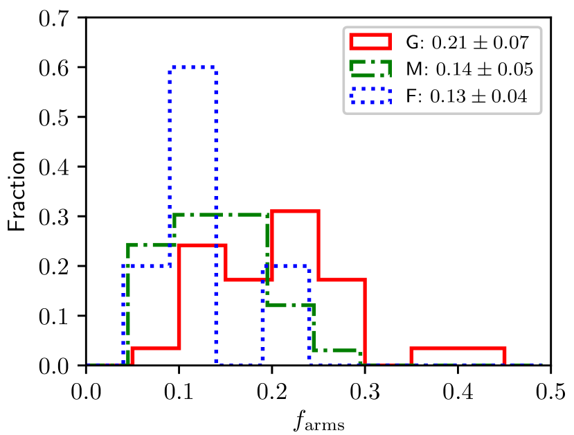
Figure 19: Distribution of the sample galaxies by their arms-to-total ratio. The red solid line depicts grand design galaxies, green dash-dotted line and blue dotted line show multi-armed and flocculent galaxies.

Fig. 19 demonstrates the distribution of the galaxies by the arms-to-total ratio in the $r$ band. Only stage 2 galaxies were used to make this plot since we need a full coverage of the spiral pattern by a spiral mask to compute a valid arms-to-total ratio (see Sect. 3.3). The mean value for all galaxies is $\left<f_{\mathrm{arms}}\right>=0.17\pm 0.07$. The grand design galaxies show, on average, brighter spirals ($\left<f_{\mathrm{arms}}\right>=0.21\pm 0.07$) than multi-armed ($\left<f_{\mathrm{arms}}\right>=0.14\pm 0.05$) and flocculent galaxies ($\left<f_{\mathrm{arms}}\right>=0.13\pm 0.04$). Similar results were reported in Kendall et al. (2011) for the NIR. They demonstrated that grand design galaxies tend to have a higher non-axisymmetric power level value, which was used as a measure of the spiral arms strength in the galaxy.

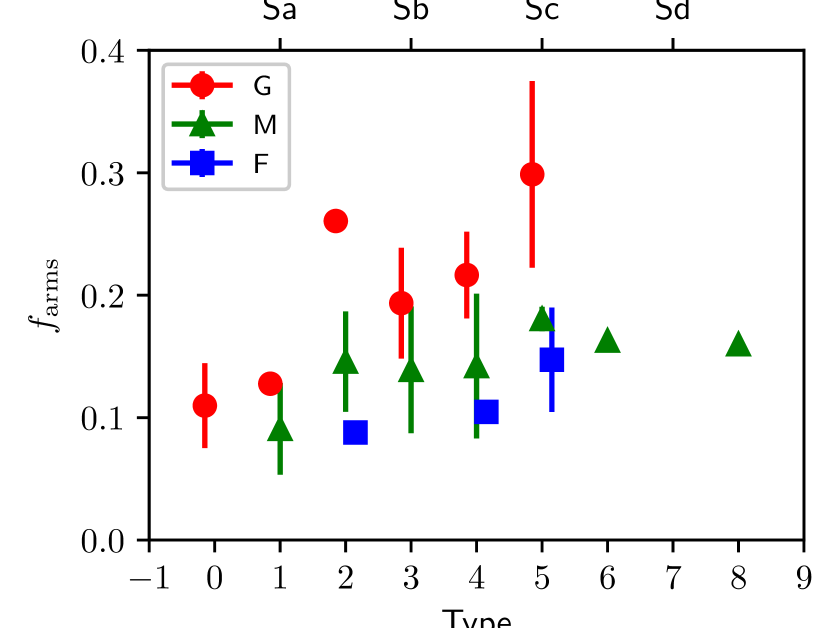
Figure 20: Dependence of the arms-to-total ratio on morphological type for grand design (red dots), multi-armed (green triangles) and flocculent (blue squares) galaxies.

Fig. 20 shows the relation between the arms-to-total ratio and Hubble type separately for grand design, multi-armed and flocculent galaxies. One can see that in the case of grand design galaxies, there is a statistically significant correlation between these parameters: the light fraction of the spiral pattern for later types is about two times larger than for earlier types. The corresponding correlation for the multi-armed galaxies is considerably weaker (the Pearson correlation coefficient is only 0.24 versus 0.66 for the grand design galaxies). The multi-armed galaxies also have a lower arms-to-total ratio than the grand design galaxies of the corresponding type. We note that in Kendall et al. (2015) it was reported that there is no obvious correlation between the Hubble type and the spiral arm strength measured by the amplitude of the $m=2$ Fourier mode.

Band	$f_{\mathrm{arm}s}^{a}$	$f_{\mathrm{arms}}^{c}$	$\kappa$
$g$	$0.13\pm 0.04$	$0.30\pm 0.10$	0.64
$r$	$0.12\pm 0.03$	$0.26\pm 0.08$	0.66
$i$	$0.12\pm 0.03$	$0.24\pm 0.08$	0.61

Table 3: Arms-to-total ratios for early (Hubble type $a$, second column) and late (Hubble type $c$, third columns) spirals in the SDSS passbands $g$, $r$ and $i$. The last column is the Pearson correlation coefficient for $T-f_{\mathrm{arms}}$ relation.

Table 3 summarises the behaviour of arms-to-total – type correlations in different passbands. One can see that for the $g$ band, both the arms-to-total ratio and the difference between early and late types is the highest. This result is in agreement with Yu et al. (2018), where they show that the strength of Fourier modes, which they used as a spiral strength measure, is systematically larger in bluer bands.

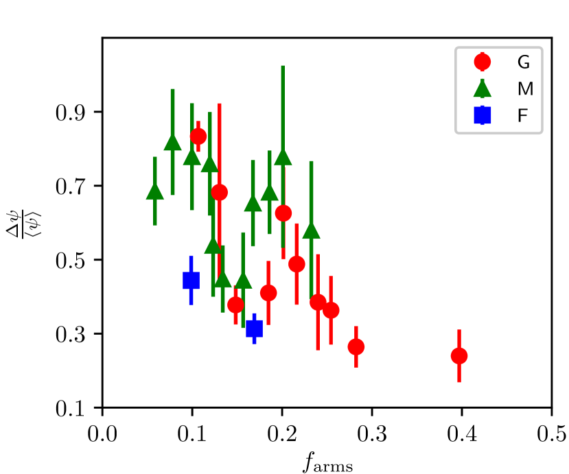
Figure 21: Pitch angle variation as a function of arms-to-total ratio in the $r$ band for grand design (red dots), multi-armed (green triangles) and flocculent (blue squares) classes of galaxies. Each point represents an averaging by three galaxies to enhance the signal-to-noise ratio.

Fig. 21 presents the pitch angle variation as an arms-to-total ratio for grand design, multi-armed and flocculent galaxies. One can see in the case of grand design spirals that there is a significant anti-correlation (the Pearson coefficient $\kappa=-0.56$) between these two quantities: brighter spirals tend to have a lower pitch angle variation (they are closer to a pure logarithmic shape) than weaker ones. On the other hand, multi-armed galaxies do not show such a correlation.

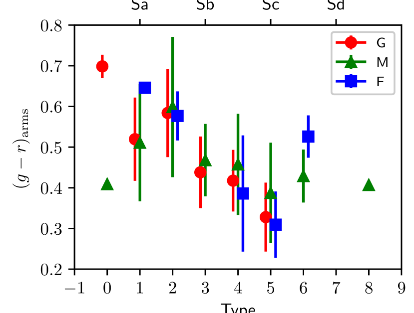
Figure 22: Colour of the spiral arms $g-r$ as a function of Hubble type for grand design (red dots), multi-armed (green triangles) and flocculent (blue squares) galaxies.

Fig. 22 demonstrates the mean $g-r$ colour of the spiral arms as a function of Hubble type. One can see that there is a statistically significant correlation between the colour of spiral structure and Hubble type for all classes of spirals, although with some outlying points due to a poor statistics in the case of flocculent galaxies. It is also worth noticing that within the same morphological type all three spiral classes may have practically the same colour. We conclude that the arms-to-total ratio and the colour of the arms have a more notable impact on the assigned Hubble type of a galaxy than the pitch angle of its spiral structure. The fraction of light in the arms and their colour could explain much about the galaxy classification, which correlates with both the characteristics of the spiral arms and the ability to recognize them and sort their properties into classes.

5 Discussion

5.1 Important issues

Here we consider how different factors may influence our results.

An important issue is how the uncertainty in the correction for the galaxy projection may potentially affect the measured quantities of the spiral structure. First, the sample galaxies are viewed almost face-on (the average inclination for our sample is $\langle\mathfrak{i}\rangle=36\pm 13\degr$, as taken from HyperLeda). In addition to that, in Sect. 4.1 we have checked that our measures of $q_{25}$ correspond well to those listed in HyperLeda. Therefore, we should not expect that a small uncertainty in the image de-projection would significantly change the results of our fitting of the spiral structure. However, to estimate this effect, we made a series of de-projections with changing the galaxy inclination within $\pm 8\degr$ and the position angle within $\pm 10\degr$ (which are conservative estimates of the errors on $\mathfrak{i}$ and $\mathrm{PA}$). We show, that the mean value of the pitch angle is almost not affected by the de-projection error: its rms value is only $\sim 2\%$. The mean dispersion of the total magnitude of the arm structure is $\approx 0.05$, the mean width varies at about 7% level. The most affected parameter is the pitch angle variation with an rms of 17%. In general, our test gave us the confidence that the variation of the estimated parameters of the spiral structure due to the de-projection errors is not significant.

As in this study we work with the optical data, the role of dust must be considered. The dust opacity is greater within spiral arms (Holwerda et al., 2005) than in the inter-arm or outside-arm disc regions. This is related to a higher surface density of molecular clouds in spiral arms and associated star formation. Notwithstanding the higher dust extinction in the spiral arms, measuring the arm pitch angle should not be affected by it as we fit the maxima on the photometric cuts perpendicular to the spiral arms and assume that most dust obscuration is located in narrow lanes alongside the inner edge of the spiral arm. Thus, we expect that there should not be a shift of the maximum emission on this cut due to the dust absorption. As our estimates of the pitch angle are consistent with the works where different approaches for tracing spiral arms are used (see Sect. 4.1), we are confident that dust does not significantly influence our measured pitch angles.

As to the arm width, arm fraction and arm colours, this statement needs to be validated. To estimate the effect of internal extinction, we adopt the following correction for the apparent disc magnitude from Driver et al. (2008) and use this value as a lower estimate for the arms: $m_{\mathrm{disc,obs}}-m_{\mathrm{disc,intrin}}=d_{1}+d_{2}\,[1-\cos(\mathfrak{i})]^{d_{3}}\,,$ where $\mathfrak{i}$ is estimated in Sect. 2.2 and the coefficients in this equation depend on wavelength and are provided in Driver et al. (2008) for various passbands, including the $g$, $r$ and $i$ wavebands. Thus, if we correct the observed total galaxy luminosity for the inclination-dependent extinction effect using $\Delta M_{r}=1.27\,(\lg q_{25})^{2}$ from Unterborn & Ryden (2008), we can estimate that the fraction of the the spiral arms is underestimated, on average, by at least 5%. The corrected colour $g-r$ appears to be shifted by at least -0.06 mag.

The influence of dust attenuation on the measurements of the arm width should be considered in great detail and will be addressed by us in a further work. Here we can only assume that its influence cannot be neglected, at least for the $w_{1}$ half-width, but, at the same time, it should not change the main result of this paper: for most sample galaxies we clearly observe an increase of the arm width with radius.

We should also note that our sample inevitably suffers from different selection effects. For example, by the construction of the sample, we undercount flocculent galaxies of later types: in our sample the average type for grand design galaxies is $\langle T\rangle=3.5\pm 1.3$, for multi-armed galaxies $\langle T\rangle=4.0\pm 1.3$, and for flocculent galaxies $\langle T\rangle=4.2\pm 1.3$. For comparison, Díaz-García et al. (2019) gives $T=3$, $T=5$ and $T=6$ for the same arm classes, but on the basis of 391 galaxies from the S⁴G survey. Thus, the results regarding the flocculent arm class in our sample should be considered with caution.

5.2 Influence of the environment on spiral structure

Here we analyse how the parameters of spiral structure depend on the environment. In Table 1 we listed the galaxy environment as belonging to a group, a triple, a group or a cluster, as well as being isolated. Here we simplify this classification to ‘isolated’ (45 galaxies) or ‘non-isolated’ (110 galaxies). In Fig. 23 we show the distributions of the sample galaxies by arm class and number of spiral arms. As one can see, the percentage of grand design spirals among the isolated galaxies is lower as compared to the non-isolated galaxies (15% versus 25%, respectively). However, the percentage of $N_{\mathrm{arms}}=2$ spirals in isolated galaxies is 47% (21 galaxies) versus 53% in non-isolated galaxies, with a slightly higher number of $N_{\mathrm{arms}}=3$ spirals (29% vesrus 22%). The lack of $N_{\mathrm{arms}}>3$ spirals can be explained by the selection effect, as we excluded many multi-armed and flocculent galaxies with indistinct spiral arms. We can conclude that in our sample the number of grand design spirals in non-isolated galaxies is slightly larger than in isolated galaxies. Interestingly, the same conclusion can be done for a larger sample of 391 galaxies from (Díaz-García et al., 2019): 17% of their grand design galaxies are isolated versus 23% of non-isolated grand design galaxies (20% of isolated galaxies have $N_{\mathrm{arms}}=2$ versus 16% of non-isolated galaxies). Also, for our sample we considered the other parameters of spiral structure (pitch angle, arm width etc.) depending on the environment, and did not find any statistically significant difference for any of them.

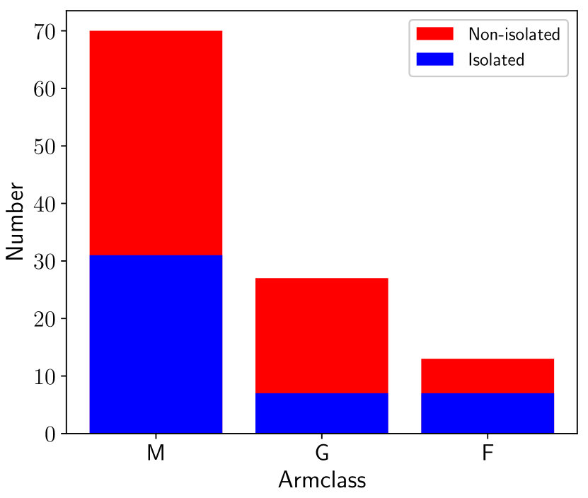
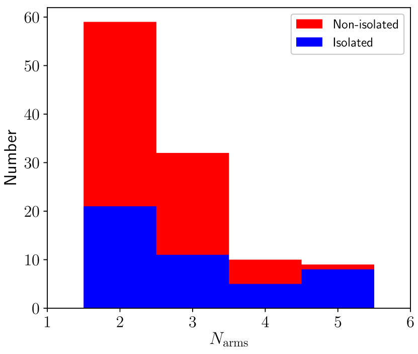
Figure 23: Distribution of the sample galaxies by arm class (leftmost panel) and arm number (rightmost panel) for isolated and non-isolated galaxies.

5.3 Dependence on wavelength

We analysed how the retrieved parameters of spiral structure vary with waveband. As the $gri$ bands are located closely to each other, we did not find any statistical difference between these bands for the pitch angle $\psi$, width $w$, width asymmetry $A$, and width slope $a$. However, as was noted in Sect. 4.4, there is a decrease of the arms fraction going from the $g$ to $i$ passband: $f_{\mathrm{arms}}^{r}=(0.91\pm 0.42)\,f_{\mathrm{arms}}^{g}$ ($\kappa=0.98$) and $f_{\mathrm{arms}}^{i}=(0.85\pm 0.51)\,f_{\mathrm{arms}}^{g}$ ($\kappa=0.96$).

5.4 Dominant mechanisms for generating spiral arms

In this paper we try to distinguish from observations between different spiral arm classes assuming that they correspond to different dominant models for generating the observed spiral structure. There have been proposed different observational tests for discriminating between, for example, the quasi-stationary density wave theory, dynamic spirals, bar-driven spirals and tidally-induced arms (see a review by Dobbs & Baba, 2014).

For explaining the large number of grand design galaxies, three possible scenarios are often discussed. In the quasi-stationary wave theory density waves are most likely to be stable in galaxies with two-armed spiral structure (Lin & Shu, 1967). Kormendy & Norman (1979) suggested that spirals can be induced by tidal interactions or can be bar driven. Elmegreen & Elmegreen (1982) found only 10% of isolated galaxies having a grand design structure, whereas flocculent galaxies are most common among isolated and barred galaxies. In our sample, we do not see such a strong difference in spiral pattern between the isolated and non-isolated galaxies: grand design galaxies are almost equally found as in groups and binaries, as in isolation. Most likely, it is related to the selection effect, as we carefully selected galaxies with a rather traceable spiral pattern and without strong interactions. Also, it should be stressed that determining truly isolated galaxies and those that have not undergone a recent merger event is not a trivial task (Verley et al., 2007), taking into account that grand design galaxies should retain their spiral structure for $\sim 1$ Gyr after an interaction (Oh et al., 2008).

Although in our study we did not study the bar parameters and their link to spiral structure (we plan to do this in a subsequent paper), we found no influence of the bar presence on all parameters of the spiral structure under study. At the same time, we find that two out of 7 isolated grand design galaxies have bars, whereas 12 galaxies out of 27 non-isolated grand design galaxies demonstrate a bar structure.

One of the most interesting results of this study is that the spiral arms in grand design galaxies have a lower difference between their overall pitch angles than in multi-armed galaxies. In the case of recent merger, which could induce a grand design spiral pattern in one of the galaxies, we can expect to see a significant difference in the pitch angles of the individual arms shortly after the interaction (see e.g. the results of modelling for M 51, Dobbs et al., 2010). However, all our grand design galaxies do not show a strong interaction, and, thus, even if a merger took place in the past, this difference could merely vanish with time. The steady-density wave theory states that all spiral arms should have the same pitch angle as the spiral pattern has the same angular speed everywhere in the galaxy. Even though the grand design galaxies in our sample show a lower difference in the pitch angles of their arms than the other two classes, this difference in significantly non-zero and is beyond the errors of the pitch angle estimation. On the other hand, the swing amplification theory does predict that the spiral arms in a galaxy may have different pitch angles: due to differential rotation, one arm can become more tightly wound as time goes by, while new spiral arms with larger pitch angles start to grow (Baba et al., 2013).

The most important characteristic, we studied in this work, is the arm width. We found, that for the vast majority of the sample galaxies the arm width steadily grows with galactocentric distance, in agreement with (Reid et al., 2014; Honig & Reid, 2015). As can be seen from simulations by (Dobbs et al., 2010), the arm width is indeed growing significantly with radius for tidally-induced spirals. On the other hand, the swing amplification scenario may also explain this trend, as ‘swinging inherently fans material outward’ (Honig & Reid 2015, see also Toomre 1981). In the quasi-stationary density wave theory this question has not been addressed.

Therefore, based on the results we obtained in this work, we cannot determine for certain which mechanisms are responsible for the observed spiral structures. A multi-wavelength study for a large sample of galaxies is highly needed where different constituents in spirals (gas, dust, stars) can be distinguished and traced.

6 Conclusions

In this paper we used SDSS $gri$-band images to perform a detailed analysis of the spiral structure in the 155 face-on non-interacting spiral galaxies. Our sample is mostly composed of multi-armed and grand design galaxies, with a fraction of flocculent galaxies, in which at least one arm could be visually traced.

In our study we used an approach of fitting an arm profile by creating a series of photometric cuts perpendicular to its direction. For tracing the spiral structure, we start from the inner galaxy region (the ends of a bar or where spirals begin to be visible beyond the main body of a bulge) to the outermost regions to which we are able to trace the spirals. Along with the pitch angle and its variation with radius, we measured, for the first time based on the spiral view in the optical, the arm width and its variation with galactocentric distance, the fraction of the spiral structure to the total galaxy luminosity, and its colour. Coupling with the arm number and the general arm class (grand design, flocculent or multi-armed), these quantities define the photometric properties of the spiral structure in galaxies, which can in principal be used to distinguish between different mechanisms of generating spiral structure in galaxies.

The main results of this paper are as follows.

1. The pitch angle does not exhibit a strong dependence on arm class: galaxies of all three classes may have a small or vice versa large pitch angle. Also, we did not find any correlation of the pitch angle with the bar presence or galaxy environment in the context of its belonging to a pair or a group, or being isolated. The difference of the pitch angle in the $gri$ bands is not significant.

2. The pitch angle demonstrates a weak correlation with morphological type in the sense that early spirals tend to be more tightly wound than the other types and late spirals may have a wide range of pitch angles. The pitch angle variation along the radius may be large (on average, approximately 50% or 7.5 deg), which is in line with previous studies by Savchenko & Reshetnikov (2013) and Díaz-García et al. (2019). It seems smaller for flocculent and grand design galaxies and larger for multi-armed galaxies. We found that grand design galaxies show a smaller difference of pitch angle for individual arms than multi-armed galaxies.

3. The arm width, normalised by the optical radius, tends to be larger for grand design galaxies and smaller for flocculent galaxies, though the significance of this difference is weak. Also, we do not find a difference between the arm classes by the width asymmetry: on average, the inner half-width $w_{1}$ is less than the outer half-width $w_{2}$, which translates into a positive asymmetry value. Also, for most sample galaxies we observe an increase of the arm width with galactocentric distance, showing no dependence on the arm class. As for the pitch angle, we find no correlation of the arm width with the waveband considered, bar presence, and galaxy environment.

4. Grand design spirals, as one would expect, contribute slightly more light to the total galaxy luminosity than the other two spiral classes. This arm fraction decreases with increasing wavelength. The average fraction for grand design galaxies $f_{\mathrm{arms}}\approx 0.2$, which in some cases may increase up to 0.4-0.5. Also, for grand design galaxies we see a strong correlation between the arms-to-total ratio and Hubble stage (late spirals have a larger fraction of the spiral pattern than early ones) and anti-correlation between the arms fraction and the pitch angle variation (more luminous spirals exhibit smaller variations of the pitch angle), whereas we do not see such a dependence for multi-armed spirals.

5. We find a tight correlation between the arm colour and morphological type: spirals become bluer in later-type galaxies for all spiral arm classes. Within one morphological type all three spiral classes do not differ significantly by their colour.

   We stress that the conclusions on the flocculent class should be considered with caution as we significantly undercount flocculent spirals in our sample.

   Observationally, based on only three optical bands and dividing galaxies into three classes by spiral pattern, we do not readily distinguish between these arm classes for the sample galaxies. The significant difference in them is only the average arm width and arm fraction, which merely reflect the scheme we used to classify the spirals. We assume that a study on a wider range of wavelengths would definitely help to find a strong observational difference between these three classes. Also a detailed look into the structure of galaxies (e.g. the view of spirals in the inner versus outer region) and the interplay between the spiral arms and main structural components (disc, bulge, bar) might shed light on this problem.

References

- Albareti et al. (2017) Albareti F. D., et al., 2017, ApJS, 233, 25
- Astropy Collaboration et al. (2013) Astropy Collaboration et al., 2013, A&A, 558, A33
- Athanassoula (2012) Athanassoula E., 2012, MNRAS, 426, L46
- Athanassoula et al. (2009a) Athanassoula E., Romero-Gómez M., Masdemont J. J., 2009a, MNRAS, 394, 67
- Athanassoula et al. (2009b) Athanassoula E., Romero-Gómez M., Bosma A., Masdemont J. J., 2009b, MNRAS, 400, 1706
- Athanassoula et al. (2010) Athanassoula E., Romero-Gómez M., Bosma A., Masdemont J. J., 2010, MNRAS, 407, 1433
- Baba et al. (2013) Baba J., Saitoh T. R., Wada K., 2013, ApJ, 763, 46
- Baillard et al. (2011) Baillard A., et al., 2011, A&A, 532, A74
- Berrier et al. (2013) Berrier J. C., et al., 2013, ApJ, 769, 132
- Bertin (2011) Bertin E., 2011, in Evans I. N., Accomazzi A., Mink D. J., Rots A. H., eds, Astronomical Society of the Pacific Conference Series Vol. 442, Astronomical Data Analysis Software and Systems XX. p. 435
- Bertin & Arnouts (1996) Bertin E., Arnouts S., 1996, A&AS, 117, 393
- Bertin et al. (1989a) Bertin G., Lin C. C., Lowe S. A., Thurstans R. P., 1989a, ApJ, 338, 78
- Bertin et al. (1989b) Bertin G., Lin C. C., Lowe S. A., Thurstans R. P., 1989b, ApJ, 338, 104
- Bertin et al. (2002) Bertin E., Mellier Y., Radovich M., Missonnier G., Didelon P., Morin B., 2002, in Bohlender D. A., Durand D., Handley T. H., eds, Astronomical Society of the Pacific Conference Series Vol. 281, Astronomical Data Analysis Software and Systems XI. p. 228
- Binney & Tremaine (2008) Binney J., Tremaine S., 2008, Galactic Dynamics: Second Edition. Princeton University Press
- Buta et al. (2015) Buta R. J., et al., 2015, ApJS, 217, 32
- Calzetti et al. (2005) Calzetti D., et al., 2005, ApJ, 633, 871
- Cohen et al. (1986) Cohen R. S., Dame T. M., Thaddeus P., 1986, ApJS, 60, 695
- Conselice (2006) Conselice C. J., 2006, MNRAS, 373, 1389
- Considere & Athanassoula (1982) Considere S., Athanassoula E., 1982, A&A, 111, 28
- Dambis et al. (2015) Dambis A. K., et al., 2015, Astronomy Letters, 41, 489
- Davis & Hayes (2014) Davis D. R., Hayes W. B., 2014, ApJ, 790, 87
- Davis et al. (2017) Davis B. L., Graham A. W., Seigar M. S., 2017, MNRAS, 471, 2187
- Díaz-García et al. (2019) Díaz-García S., Salo H., Knapen J. H., Herrera-Endoqui M., 2019, arXiv e-prints, p. arXiv:1908.04246
- Dobbs & Baba (2014) Dobbs C., Baba J., 2014, Publ. Astron. Soc. Australia, 31, e035
- Dobbs et al. (2010) Dobbs C. L., Theis C., Pringle J. E., Bate M. R., 2010, MNRAS, 403, 625
- Driver et al. (2008) Driver S. P., Popescu C. C., Tuffs R. J., Graham A. W., Liske J., Baldry I., 2008, ApJ, 678, L101
- Elmegreen (1990) Elmegreen B. G., 1990, Annals of the New York Academy of Sciences, 596, 40
- Elmegreen (2011) Elmegreen B. G., 2011, in Charbonnel C., Montmerle T., eds, EAS Publications Series Vol. 51, EAS Publications Series. pp 19–30 (arXiv:1101.3109), doi:10.1051/eas/1151002
- Elmegreen (2015) Elmegreen D. M., 2015, Galaxy Morphology at High Redshift. p. 455, doi:10.1007/978-3-319-10614-4_37
- Elmegreen & Elmegreen (1982) Elmegreen D. M., Elmegreen B. G., 1982, MNRAS, 201, 1021
- Elmegreen & Elmegreen (1987) Elmegreen D. M., Elmegreen B. G., 1987, ApJ, 314, 3
- Elmegreen et al. (1991) Elmegreen D. M., Sundin M., Elmegreen B., Sundelius B., 1991, A&A, 244, 52
- Elmegreen et al. (2005) Elmegreen D. M., Elmegreen B. G., Rubin D. S., Schaffer M. A., 2005, ApJ, 631, 85
- Elmegreen et al. (2011) Elmegreen D. M., et al., 2011, ApJ, 737, 32
- Engargiola et al. (2003) Engargiola G., Plambeck R. L., Rosolowsky E., Blitz L., 2003, ApJS, 149, 343
- Font et al. (2019) Font J., Beckman J. E., James P. A., Patsis P. A., 2019, MNRAS, 482, 5362
- Forgan et al. (2018) Forgan D. H., Ramón-Fox F. G., Bonnell I. A., 2018, MNRAS, 476, 2384
- Foyle et al. (2010) Foyle K., Rix H. W., Walter F., Leroy A. K., 2010, ApJ, 725, 534
- Freeman (1970) Freeman K. C., 1970, ApJ, 160, 811
- Georgelin & Georgelin (1976) Georgelin Y. M., Georgelin Y. P., 1976, A&A, 49, 57
- Gerola & Seiden (1978) Gerola H., Seiden P. E., 1978, ApJ, 223, 129
- Goldreich & Tremaine (1978) Goldreich P., Tremaine S., 1978, ApJ, 222, 850
- Grabelsky et al. (1987) Grabelsky D. A., Cohen R. S., Bronfman L., Thaddeus P., May J., 1987, ApJ, 315, 122
- Grosbøl & Dottori (2012) Grosbøl P., Dottori H., 2012, A&A, 542, A39
- Harsoula & Kalapotharakos (2009) Harsoula M., Kalapotharakos C., 2009, MNRAS, 394, 1605
- Hart et al. (2016) Hart R. E., et al., 2016, MNRAS, 461, 3663
- Hart et al. (2017a) Hart R. E., Bamford S. P., Casteels K. R. V., Kruk S. J., Lintott C. J., Masters K. L., 2017a, MNRAS, 468, 1850
- Hart et al. (2017b) Hart R. E., et al., 2017b, MNRAS, 472, 2263
- Holmberg (1941) Holmberg E., 1941, ApJ, 94, 385
- Holwerda et al. (2005) Holwerda B. W., González R. A., van der Kruit P. C., Allen R. J., 2005, A&A, 444, 109
- Honig & Reid (2015) Honig Z. N., Reid M. J., 2015, ApJ, 800, 53
- Hou et al. (2009) Hou L. G., Han J. L., Shi W. B., 2009, A&A, 499, 473
- Hubble (1936) Hubble E. P., 1936, Realm of the Nebulae
- Jedrzejewski (1987) Jedrzejewski R. I., 1987, MNRAS, 226, 747
- Julian & Toomre (1966) Julian W. H., Toomre A., 1966, ApJ, 146, 810
- Kalnajs (1973) Kalnajs A. J., 1973, Proceedings of the Astronomical Society of Australia, 2, 174
- Karapetyan et al. (2018) Karapetyan A. G., Hakobyan A. A., Barkhudaryan L. V., Mamon G. A., Kunth D., Adibekyan V., Turatto M., 2018, MNRAS, 481, 566
- Kaufmann & Contopoulos (1996) Kaufmann D. E., Contopoulos G., 1996, A&A, 309, 381
- Kendall et al. (2008) Kendall S., Kennicutt R. C., Clarke C., Thornley M. D., 2008, MNRAS, 387, 1007
- Kendall et al. (2011) Kendall S., Kennicutt R. C., Clarke C., 2011, MNRAS, 414, 538
- Kendall et al. (2015) Kendall S., Clarke C., Kennicutt R. C., 2015, MNRAS, 446, 4155
- Kennicutt (1981) Kennicutt R. C. J., 1981, AJ, 86, 1847
- Kormendy & Norman (1979) Kormendy J., Norman C. A., 1979, ApJ, 233, 539
- Law et al. (2012) Law D. R., Shapley A. E., Steidel C. C., Reddy N. A., Christensen C. R., Erb D. K., 2012, Nature, 487, 338
- Lin & Shu (1964) Lin C. C., Shu F. H., 1964, ApJ, 140, 646
- Lin & Shu (1967) Lin C. C., Shu F. H., 1967, in van Woerden H., ed., IAU Symposium Vol. 31, Radio Astronomy and the Galactic System. p. 313
- Lintott et al. (2008) Lintott C. J., et al., 2008, MNRAS, 389, 1179
- Lynds (1970) Lynds B. T., 1970, in Becker W., Kontopoulos G. I., eds, IAU Symposium Vol. 38, The Spiral Structure of our Galaxy. p. 26
- Ma (2001) Ma J., 2001, Chinese J. Astron. Astrophys., 1
- Ma (2002) Ma J., 2002, A&A, 388, 389
- Makarov et al. (2014) Makarov D., Prugniel P., Terekhova N., Courtois H., Vauglin I., 2014, A&A, 570, A13
- Masters et al. (2010) Masters K. L., et al., 2010, MNRAS, 405, 783
- Masters et al. (2019) Masters K. L., et al., 2019, MNRAS, 487, 1808
- Muñoz-Mateos et al. (2015) Muñoz-Mateos J. C., et al., 2015, ApJS, 219, 3
- Oh et al. (2008) Oh S. H., Kim W.-T., Lee H. M., Kim J., 2008, ApJ, 683, 94
- Price-Whelan et al. (2018) Price-Whelan A. M., et al., 2018, AJ, 156, 123
- Puerari & Dottori (1992) Puerari I., Dottori H. A., 1992, A&AS, 93, 469
- Puerari et al. (2014) Puerari I., Elmegreen B. G., Block D. L., 2014, AJ, 148, 133
- Regan & Wilson (1993) Regan M. W., Wilson C. D., 1993, AJ, 105, 499
- Reid et al. (2014) Reid M. J., et al., 2014, ApJ, 783, 130
- Salo & Laurikainen (2000) Salo H., Laurikainen E., 2000, MNRAS, 319, 377
- Sánchez-Menguiano et al. (2017) Sánchez-Menguiano L., et al., 2017, A&A, 603, A113
- Savchenko & Reshetnikov (2013) Savchenko S. S., Reshetnikov V. P., 2013, MNRAS, 436, 1074
- Schlafly & Finkbeiner (2011) Schlafly E. F., Finkbeiner D. P., 2011, ApJ, 737, 103
- Seiden & Gerola (1979) Seiden P. E., Gerola H., 1979, ApJ, 233, 56
- Seigar & James (1998) Seigar M. S., James P. A., 1998, MNRAS, 299, 685
- Seigar et al. (2005) Seigar M. S., Block D. L., Puerari I., Chorney N. E., James P. A., 2005, MNRAS, 359, 1065
- Seigar et al. (2006) Seigar M. S., Bullock J. S., Barth A. J., Ho L. C., 2006, ApJ, 645, 1012
- Seigar et al. (2008) Seigar M. S., Kennefick D., Kennefick J., Lacy C. H. S., 2008, ApJ, 678, L93
- Sheth et al. (2010) Sheth K., et al., 2010, PASP, 122, 1397
- Shields et al. (2015) Shields D. W., et al., 2015, arXiv e-prints, p. arXiv:1511.06365
- Skowron et al. (2019) Skowron D. M., et al., 2019, Science, 365, 478
- Tempel et al. (2012) Tempel E., Tago E., Liivamägi L. J., 2012, A&A, 540, A106
- Thornley (1996) Thornley M. D., 1996, ApJ, 469, L45
- Toomre (1969) Toomre A., 1969, ApJ, 158, 899
- Toomre (1981) Toomre A., 1981, in Fall S. M., Lynden-Bell D., eds, Structure and Evolution of Normal Galaxies. pp 111–136
- Toomre & Toomre (1972) Toomre A., Toomre J., 1972, ApJ, 178, 623
- Unterborn & Ryden (2008) Unterborn C. T., Ryden B. S., 2008, ApJ, 687, 976
- Vallée (2005) Vallée J. P., 2005, AJ, 130, 569
- Verley et al. (2007) Verley S., et al., 2007, A&A, 472, 121
- Vogel et al. (1988) Vogel S. N., Kulkarni S. R., Scoville N. Z., 1988, Nature, 334, 402
- Wiklind et al. (1990) Wiklind T., Rydbeck G., Hjalmarson A., Bergman P., 1990, A&A, 232, L11
- York et al. (2000) York D. G., et al., 2000, AJ, 120, 1579
- Yu & Ho (2019) Yu S.-Y., Ho L. C., 2019, ApJ, 871, 194
- Yu et al. (2018) Yu S.-Y., Ho L. C., Barth A. J., Li Z.-Y., 2018, ApJ, 862, 13
- Yuan & Grosbol (1981) Yuan C., Grosbol P., 1981, ApJ, 243, 432
- de Lapparent et al. (2011) de Lapparent V., Baillard A., Bertin E., 2011, A&A, 532, A75