A universal formula for the relativistic correction to the mutual friction coupling time-scale in neutron stars

Abstract

Vortex mediated mutual friction governs the coupling between the superfluid and normal components in neutron star interiors. By, for example, comparing precise timing observations of pulsar glitches with theoretical predictions it is possible to constrain the physics in the interior of the star, but to do so an accurate model of the mutual friction coupling in General Relativity is needed. We derive such a model directly from Carter’s multi-fluid formalism, and study the vortex structure and coupling timescale between the components in a relativistic star. We calculate how General Relativity modifies the shape and the density of the quantised vortices and show that, in the quasi-Schwarzschild coordinates, they can be approximated as straight lines for realistic neutron star configurations. Finally, we present a simple universal formula (given as a function of the stellar compactness alone) for the relativistic correction to the glitch rise-time, which is valid under the assumption that the superfluid reservoir is in a thin shell in the crust or in the outer core. This universal relation can be easily employed to correct, a posteriori, any Newtonian estimate for the coupling time scale, without any additional computational expense.

1 Introduction

Pulsars are known to be among the most stable clocks in the universe, but their timing irregularities can help unveil the mystery of their interior structure. The sudden spin-up events called glitches are thought to be a manifestation of the presence of a neutron superfluid in the interior of the neutron star (Anderson & Itoh, 1975). According to this theory, there is a region of the star, the exact nature and extension of which is still uncertain (Andersson et al., 2012; Chamel, 2013), in which the quantised vortices of the superfluid are mostly pinned to the normal component during almost the whole life of the neutron star (Alpar, 1977; Epstein & Baym, 1988). This results in the formation of an angular momentum reservoir which, when the lag between the superfluid and the normal component becomes too large, is released in a catastrophic event, producing the glitch (for a recent review see Haskell & Melatos 2015).

Many attempts to constrain the physical properties of neutron stars from observations of the relaxation process have already been made (Baym et al., 1969; Datta & Alpar, 1993; Link et al., 1999; Graber et al., 2018), but with the development of the Square Kilometer Array (Lazio, 2009; Weltman et al., 2018) and the Five-hundred-meter Aperture Spherical Telescope (Nan et al., 2011), we will have access to precisions which have never been explored.

The improvement of the resolution of pulsar timing techniques has already made it possible to have information about the first seconds of a glitch (Palfreyman et al., 2018) allowing, also, to fit the profile of the rise with simple theoretical models (Ashton et al., 2019; Pizzochero et al., 2019) and constrain the glitch rise-time. In particular, the observation of the largest glitch of the Crab pulsar (Shaw et al., 2018) has also allowed to put constraints on the mutual friction parameters (Haskell et al., 2018). Furthermore, the coupling between the superfluid and the normal fluid plays a key role when extracting nuclear physics parameters related to the equation of state from measurements of the activity of a pulsar (Newton et al., 2015). Precise measurements of the activity can also be used to constrain the mass of a pulsar (Ho et al., 2015; Pizzochero et al., 2017). Thus, it is becoming increasingly important to have models which are able to produce quantitative predictions for the coupling time-scale between the normal and the superfluid component.

General Relativity plays a fundamental role in neutron star theory as it is not possible to obtain realistic predictions for masses and radii in a merely Newtonian context (Shapiro & Teukolsky, 1983). This implies that any quantitative study, whose results depend on the structure of the neutron star, must be performed considering the density profile to be a solution of the Tolman-Oppenheimer-Volkoff (TOV) equations, making non-relativistic models inconsistent. Furthermore, Rothen (1981) has shown, for a simplified constant density neutron star model, that the spacetime curvature can affect significantly the geometry of the vortex lines and this can have consequences on the estimates of the mutual friction. In addition, the difference of speed between the clocks on the Earth and the clocks in the neutron star, due to the gravitational redshift phenomenon, influences every dynamical time-scale we observe. It is clear, then, that to make quantitative predictions of the glitch rise-time, it is necessary to have an estimate of the relativistic effects. An initial study was performed by Sourie et al. (2017) for a system composed of two rigid components, and significant quantitative differences (a correction of the order of $40\%$) were found with respect to Newtonian models for selected equations of state.

Here, our final objective is to construct a consistent general relativistic model for the mutual friction coupling in neutron stars, that can be applied to pulsar glitches, r-mode damping (Haskell, 2015), asteroseismology and to the study of gravitational wave emission (Glampedakis & Gualtieri, 2018). Thus, with the aim of quantifying the role of General Relativity, in this paper we will derive directly from Carter’s multifluid formalism a local simple formula for the relativistic corrections to the coupling time. To achieve this goal we will also extend the vortex-tracing technique developed by Rothen (1981) to make it applicable to the computation of the vortex density. Finally, using the conservation of the angular momentum, we will find a formula for the correction to the glitch rise-times. A key ingredient which makes this formula a universal relation (namely, the correction factor is independent on the choice of the equation of state) is the assumption that the angular momentum reservoir is located in a thin shell near the surface encompassing the crust and possibly parts of the outer core (Ho et al., 2015). This puts our results in contrast to Sourie et al. (2017), where it is assumed that the reservoir is extended over the whole core.

In the derivation of the formula we follow a sequence of five steps which cover the different aspects of the problem.

Section 2: We review the basic ideas of Carter’s hydrodynamic formalism and of the prescription for vortex-mediated mutual friction of Langlois et al. (1998), recasting the equations in a form which is convenient for our purposes.

Section 3: We study the general mathematical properties of the macroscopic vorticity of a circularly rotating non-turbulent superfluid in a stationary axisymmetric system, deriving simple techniques to compute the vortex shape and density.

Section 4: The techniques developed in the previous section are applied to the case of the neutron superfluid in a star. We derive analytic formulas for the vortex density and shape in the slow rotation approximation, and compare our results with Rothen (1981). The approximations proposed in Ravenhall & Pethick (1994) are used to simplify the expressions, unveiling their physical interpretation.

Section 5: We employ the results of the previous sections to see how the rise-time of a glitch is modified by General Relativity. Using the universality relation proposed in Breu & Rezzolla (2016) for the moment of inertia, we show that the relativistic factor we obtain is a pure function of the compactness of the star, so it is independent from the equation of state.

Section 6: We show that the universality of the relativistic correction is a direct cosequence of the assumption that the free superfluid is located in a thin shell near the surface. This is done by proving that the formula for the rise-time found by Sourie et al. (2017) reduces to ours in this limit.

Throughout the paper we adopt the spacetime signature $(-,+,+,+)$, choose units with the speed of light $c=1$ and Newton’s constant $G=1$, use greek letters $\nu$, $\rho$, $\sigma$… for coordinate tensor indexes. The sign of the volume form is chosen according to the convention $\varepsilon_{0123}=\sqrt{-g}$.

2 Relativistic vorticity and mutual friction

We briefly introduce the two-fluid formalism to model the dynamics of superfluid neutron star interiors. The coupling between the two fluids is provided by the vortex-mediated mutual friction, for which we adopt the prescription of Langlois et al. (1998), rewriting it in a form which is convenient for our purposes. To make the physical interpretation of the mutual friction clear, in subsection 2.2 we review the geometric properties of the macroscopic vorticity in General Relativity.

2.1 The two-fluid formalism

A realistic hydrodynamic description of a neutron star should take into account the existence of four components: $n_{p}^{\nu}$, the normal four-current, $n_{n}^{\nu}$, the four-current of the superfluid neutrons, $s^{\nu}$, the entropy four-current, and an electromagnetic component (Haskell & Sedrakian, 2017; Chamel, 2017). It is useful to introduce the rest-frame density associated with each component, in particular

$$n_{p}=\sqrt{-n_{p}^{\nu}n_{p\nu}}\quad\quad\quad n_{n}=\sqrt{-n_{n}^{\nu}n_{n\nu}},$$ (1)

and the four-velocities

$$u_{p}^{\nu}\,=\,n_{p}^{\nu}/n_{p}\quad\quad\quad u_{n}^{\nu}\,=\,n_{n}^{\nu}/n_{n},$$ (2)

which are clearly normalized to $-1$.

The conservation of the baryon number implies that

$$\nabla_{\nu}(n_{p}^{\nu}+n_{n}^{\nu})=0$$ (3)

and the second law of thermodynamics requires $\nabla_{\nu}s^{\nu}\geq 0$. In the following we will assume, either because chemical equilibrium is reached, or because the hydrodynamic processes considered are faster than the time-scale of the reaction (Gavassino & Antonelli, 2019), that

$$\nabla_{\nu}n_{p}^{\nu}=-\nabla_{\nu}n_{n}^{\nu}=0\,.$$ (4)

The hydrodynamic description must be consistent with the Einstein equations,

$$G^{\nu\rho}=8\pi T^{\nu\rho}_{(tot)},$$ (5)

where $G_{\nu\rho}$ is the Einstein tensor and $T_{(tot)}^{\nu\rho}$ is the total energy-momentum tensor accounting for the presence of all the four components. To recover a two-component model for a neutron star interior we split the energy-momentum tensor as

$$T_{(tot)}^{\nu\rho}=T^{\nu\rho}+T_{(ext)}^{\nu\rho}\,,$$ (6)

where $T^{\nu\rho}$ represents the fluid contribution obtained by using a two-fluid zero-temperature formalism of the kind employed by e.g. Andersson & Comer (2001). In this theory the equation of state is given in terms of a master function (Carter, 1989; Andersson & Comer, 2007)

$$-\mathcal{E}(n_{p}^{2},n_{n}^{2},n_{np}^{2}),$$ (7)

with $n_{np}^{2}=-n_{n}^{\nu}n_{p\nu}$, leading to the definition of the momenta per particle

$$\mu_{\nu}^{p}=-\dfrac{\partial\mathcal{E}}{\partial n_{p}^{\nu}}\quad\quad\quad\mu_{\nu}^{n}=-\dfrac{\partial\mathcal{E}}{\partial n_{n}^{\nu}},$$ (8)

of the generalised pressure

$$\Psi=-\mathcal{E}-n_{p}^{\nu}\mu_{\nu}^{p}-n_{n}^{\nu}\mu_{\nu}^{n}$$ (9)

and of the fluid stress-energy tensor

$$T\indices{{}^{\nu}_{\rho}}=\Psi\delta\indices{{}^{\nu}_{\rho}}+n_{p}^{\nu}\mu_{\rho}^{p}+n_{n}^{\nu}\mu_{\rho}^{n}.$$ (10)

The tensor $T_{(ext)}^{\nu\rho}$, on the other hand, contains all the contributions which are not considered in $T^{\nu\rho}$, such as the finite temperature corrections due to the presence of $s^{\nu}$, the elastic part of the stress tensor in the crust and the electromagnetic energy-momentum. These parts play a negligible role in (5), but they are fundamental in the study of the dynamics of $n^{\nu}_{p}$ and $n_{n}^{\nu}$. Taking the four-divergence of (5) and (6), we have

$$\nabla_{\rho}T\indices{{}^{\rho}_{\nu}}=f_{(ext)\nu}\,,$$ (11)

where the external force density is defined as

$$f_{(ext)}^{\nu}:=-\nabla_{\rho}T^{\nu\rho}_{(ext)}\,.$$ (12)

As a result, we have that a mixture of charged, superfluid and possibly solid components at finite temperature can be conveniently described in terms of a zero-temperature two-fluid model subject to the action of an external force.

In glitch models of the kind pioneered by Baym et al. (1969), the external force is expected to play two main roles (see e.g. the discussion in Antonelli & Pizzochero, 2017). Firstly, there is a contribution in $f^{\nu}_{(ext)}$ that is assumed to enforce the proton-electron fluid and the crustal lattice rigid rotation: this is implicitly incorporated into glitch models by imposing that $\Omega_{p}$, the angular velocity of the normal $p$ component, depends only on time. Secondly, it exerts a torque on the two-fluid system, which can be interpreted as the local contribution to the braking torque, which is included into the evolution equation for the total angular momentum of the neutron star.

2.2 The macroscopic vorticity of a superfluid

At the mesoscopic scale, the momentum $\mu^{n}_{\nu}$ is related to the superfluid order parameter $\phi$ according to the Josephson relation (Carter et al., 2006)

$$\mu^{n}_{\nu}=\dfrac{k}{2\pi}\partial_{\nu}\phi\,,$$ (13)

where $k=\pi\hbar$ to account for the Cooper pairing mechanism (if the superfluid were a Boson fluid, then $k=2\pi\hbar$). On scales smaller than the inter-vortex separation, the relation (13) implies that the four-vorticity

$$\varpi_{\nu\rho}:=(d\mu^{n})_{\nu\rho}$$ (14)

must be concentrated into vortex filaments and zero elsewhere. However, in an astrophysical context we are interested in the dynamics of macroscopic matter elements crossed by several quantised vortices. Hence, we must locally average the momentum, and the relative vorticity, over a portion of fluid. In this way, if the vortex filaments are arranged in a tangled configuration (as is expected if quantum turbulence develops in neutron star interiors, Greenstein (1970); Andersson et al. (2007)), then it is in general not possible to reconstruct the vortex line configuration starting from the knowledge of the macroscopic vorticity field.

For simplicity, we assume that turbulence is absent, so that the quantized vortices in each local matter element are parallel to each other. Given this condition, the region of spacetime occupied by the superfluid can be foliated by two-dimensional worldsheets which follow the profile of the vortex lines. Stachel (1980) has shown that these spacetime foliations are completely described by a bivector field $\mathcal{S}^{\nu\rho}$ (normalized as $\mathcal{S}^{\nu\rho}\mathcal{S}_{\nu\rho}=-2$) such that

$${\star}\mathcal{S}_{\nu\rho}\,\mathcal{S}^{\rho\sigma}=0$$ (15)

and

$${\star}\mathcal{S}_{\nu\rho}\,\partial_{\sigma}\mathcal{S}^{\rho\sigma}=0\,,$$ (16)

where the symbol ${\star}$ is the Hodge duality operator, which acts on a generic p-form $\Sigma$ as

$${\star}\Sigma_{\nu_{1}...\nu_{4-p}}=\dfrac{1}{p!}\varepsilon^{\lambda_{1}...\lambda_{p}}_{\phantom{\lambda_{1}...\lambda_{p}}\nu_{1}...\nu_{4-p}}\Sigma_{\lambda_{1}...\lambda_{p}}\,.$$ (17)

Equation (15) is an algebraic degeneracy condition: it tells us that $\mathcal{S}^{\nu\rho}$, as seen as an antisymmetric $4\times 4$ matrix, must have rank 2. This implies that the bivector $\mathcal{S}^{\nu\rho}$ is simple, i.e. there are two vector fields, say $u_{C}$ and $v_{C}$, such that

$$\mathcal{S}^{\nu\rho}\,=\,u_{C}^{\nu}\,v_{C}^{\rho}-u_{C}^{\rho}\,v_{C}^{\nu}.$$ (18)

The factor of two in the normalization condition implies that we can impose $u_{C}$ and $v_{C}$ to be orthonormal, while the minus sign tells us that one of the two vectors, conventionally $u_{C}$, is timelike. This bivector represents the unit surface element of the wordsheet and the condition (16) is the requirement that all these surface elements mesh together smoothly.

It is easy to verify that if we want the macroscopic four-vorticity $\varpi_{\nu\rho}$ to come from an array of vortices which have the shape given by $\mathcal{S}$, then it must be true that

$$\mathcal{S}^{\nu\rho}=-\dfrac{{\star}\varpi^{\nu\rho}}{\varpi}\quad\quad\quad\text{with}\quad\quad\quad\varpi:=\sqrt{\dfrac{\varpi_{\lambda\sigma}\varpi^{\lambda\sigma}}{2}}.$$ (19)

Equation (19) can be rewritten into the form

$$\varpi_{\nu\rho}\,=\,\varpi\,{\star}\mathcal{S}_{\nu\rho}\,=\,\varpi\,\varepsilon_{\nu\rho\sigma\lambda}\,u_{C}^{\sigma}\,v_{C}^{\lambda}\,,$$ (20)

so that the kernel of $\varpi_{\nu\rho}$ corresponds to the linear combinations of $u_{C}$ and $v_{C}$. The above relation allows to rewrite (15) as

$$\varpi_{\nu\rho}\,\mathcal{S}^{\rho\sigma}\,=\,0\,,$$ (21)

which naturally leads to define the two orthogonal projectors

$$\mathbin{\,\!/\mkern-5.0mu/\!}\,\indices{{}^{\nu}_{\rho}}:=\mathcal{S}^{\nu\lambda}\mathcal{S}_{\lambda\rho}\quad\quad\quad{\perp}\indices{{}^{\nu}_{\rho}}:=\dfrac{\varpi^{\nu\lambda}\varpi_{\rho\lambda}}{\varpi^{2}}\,.$$ (22)

In appendix A we show that, given an observer $\mathcal{O}$ with four-velocity $u_{\mathcal{O}}$, the vector

$$\varpi_{\mathcal{O}}^{\nu}=\varpi\,\mathcal{S}^{\nu\rho}u_{\mathcal{O}\rho}$$ (23)

can be interpreted as

$$\varpi_{\mathcal{O}}^{\nu}\,=\,k\,\mathfrak{N}_{\mathcal{O}}\,v_{\mathcal{O}}^{\nu}\,,$$ (24)

where $\mathfrak{N}_{\mathcal{O}}$ is the local surface density of vortices measured by $\mathcal{O}$ and $v_{\mathcal{O}}^{\nu}$ is the unit vector directed along the local vortex array, as seen by $\mathcal{O}$. Furthermore, the vector

$$u_{{V\mathcal{O}}}:=\dfrac{\mathbin{\,\!/\mkern-5.0mu/\!}\,u_{\mathcal{O}}}{\sqrt{-g(\mathbin{\,\!/\mkern-5.0mu/\!}\,u_{\mathcal{O}},\mathbin{\,\!/\mkern-5.0mu/\!}\,u_{\mathcal{O}})}}$$ (25)

defines the four-velocity of the vortices in the frame of $\mathcal{O}$. This velocity is constructed in a way that the relative three-velocity between the lines and the observer $\mathcal{O}$,

$$w_{V{\mathcal{O}}}:=\dfrac{u_{V{\mathcal{O}}}}{\Gamma_{V{\mathcal{O}}}}-u_{\mathcal{O}},$$ (26)

is orthogonal to the vortex lines. Here, $\Gamma_{V\mathcal{O}}=-g(u_{\mathcal{O}},u_{V\mathcal{O}})$ is the Lorentz factor associated with the relative speed $\Delta_{V\mathcal{O}}=\sqrt{g(w_{V{\mathcal{O}}},w_{V{\mathcal{O}}})}$ between $u_{\mathcal{O}}$ and $u_{V\mathcal{O}}$. As it is explained in appendix A, this Lorentz factor accounts for the length contraction phenomenon in the definition of the vortex density $\mathfrak{N}_{\mathcal{O}}$ measured by the observer $\mathcal{O}$, namely

$$\mathfrak{N}_{\mathcal{O}}\,=\,\mathfrak{N}\,\Gamma_{V{\mathcal{O}}}\,,$$ (27)

where

$$\mathfrak{N}=\sqrt{\dfrac{\varpi_{\lambda\sigma}\varpi^{\lambda\sigma}}{2\,k^{2}}},$$ (28)

can be interpreted as the rest-frame vortex density.

Despite having used a terminology related to the presence of quantised vortex lines in a superfluid, we end this subsection by remarking that the construction described so far can be applied to a more general class of fluids. In all situations in which $\varpi_{\nu\rho}$ can be computed as the exterior derivative of $\mu^{n}_{\nu}$, it is possible to use the fact $(d\varpi)_{\nu\rho\sigma}=0$ to prove that (15) implies (16). This means that a given field $\varpi_{\nu\rho}$ defines a worldsheet foliation if and only if there exists a time-like vector field $u_{C}$ such that

$$u_{C}^{\rho}\varpi_{\rho\nu}=0\,.$$ (29)

Therefore, given an arbitrary fluid for which the above equation is satisfied, it is possible to replace the words vortex line with macroscopic vorticity line everywhere in this subsection. This result is discussed in detail in appendix C by taking advantage of the language of force-free magnetohydrodynamics, based on the fact that reading the momentum $\mu^{n}_{\nu}$ as a vector potential leads to interpret the quantities introduced in equations (23) and (26) as the magnetic field and the drift velocity respectively.

2.3 The mutual friction coupling

A model for the vortex-mediated mutual friction is one of the most important elements in pulsar glitch modelling. In this work we follow the mutual friction prescription of Langlois et al. (1998), which we briefly rederive with a geometrical argument. According to Langlois et al. (1998), the tensorial quantity

$$f_{M\nu}:=-n_{n}^{\rho}\varpi^{n}_{\rho\nu}$$ (30)

provides the relativistic generalization of the Magnus force density (see also Carter et al., 2001; Andersson et al., 2016). The minus sign is chosen in a way that $f_{M}/\mathfrak{N}$ can be interpreted as the force per unit length exerted by the superfluid on the normal matter inside the core of the vortex. The norm of $f_{M}$ is

$$|f_{M}|\,=\,\sqrt{f_{M\rho}f_{M}^{\rho}}\,=\,n_{n}\,k\,\mathfrak{N}\,\Gamma_{Vn}\,\Delta_{Vn}\,,$$ (31)

in accordance with what it is expected by considering that $\mathfrak{N}_{n}=\mathfrak{N}\,\Gamma_{Vn}$ is the density of vortices measured in the frame defined by $u_{n}$, see equation (27). Regarding the direction of $f_{M}$, it is immediate to see that it is orthogonal to $u_{C}$, $v_{C}$ and $u_{n}$.

In the presence of a normal component, the vortex lines experience also a drag force per unit length (Donnelly, 1991), that we will indicate as $\mathcal{F}_{D}$. To understand how this dissipative force can be modelled it is convenient to work in the frame defined by the four-velocity

$$u_{Vp}=\dfrac{\mathbin{\,\!/\mkern-5.0mu/\!}\,u_{p}}{\sqrt{-g(\mathbin{\,\!/\mkern-5.0mu/\!}\,u_{p},\mathbin{\,\!/\mkern-5.0mu/\!}\,u_{p})}}=:u_{v}\,.$$ (32)

In this frame the vortices are at rest and the normal component moves orthogonally to the vortex lines, see the previous section. The vector $u_{Vp}$ can be interpreted as the proper four-velocity of the vortices, so, for notational convenience, it will be referred to as $u_{v}$, in full analogy with the notation used for $u_{n}$ and $u_{p}$.

Since the drag force on vortices has to balance the Magnus force (because the vortex lines have no inertia), it must be orthogonal to the vortex worldsheet. Assuming a viscous drag force per unit length $\mathcal{F}_{D}$ which is proportional to the three-velocity of the normal component in the frame of $u_{v}$, this results in

$$\mathcal{F}_{D}=\alpha\,\Gamma_{vp}^{-1}\,{\perp}u_{p}\,,$$ (33)

where $\alpha$ is a coefficient that sets the strength of the microscopic dissipative interaction between a vortex core and the constituents of the normal component.

The averaged force per unit volume $f_{D}$ is found by multiplying the force exerted on a vortex by the number $\mathfrak{N}_{p}$ of vortices per unit area in the frame defined by $u_{p}$,

$$f_{D\nu}\,=\,\mathfrak{N}_{p}\,\mathcal{F}_{D\nu}\,=\,\alpha\,\mathfrak{N}\,{\perp}\indices{{}^{\rho}_{\nu}}u_{p\rho}\,,$$ (34)

see equation (27). Hence, it is possible to write the force balance

$$f_{M}+f_{D}=0\,,$$ (35)

which, defined the dimensionless factor

$$\mathcal{R}\,:=\,\alpha\,/(k\,n_{n})\,,$$ (36)

takes the form

$$u_{n}^{\rho}\,\varpi^{n}_{\rho\nu}\,=\,\mathcal{R}\,k\,\mathfrak{N}\,{\perp}_{\nu\rho}u_{p}^{\rho},$$ (37)

which is the one proposed in Langlois et al. (1998). This equation, despite being clear from the geometrical point of view, is not written in the best form for practical purposes. By using the two orthonormal generators of $\mathcal{S}$, i.e. $u_{v}$ and $v_{p}$ , equation (37) can be cast as

$$-\varepsilon_{\nu\mu\rho\sigma}u_{n}^{\mu}u_{v}^{\rho}v_{p}^{\sigma}=\mathcal{R}(u_{p\nu}-\Gamma_{vp}u_{v\nu}).$$ (38)

In appendix B we show how to remove the dependence on $u_{v}$, so that the mutual friction is expressed in terms of the relative velocity between the $n$ and $p$ components. This procedure gives

$$-u_{n}^{\rho}\varpi^{n}_{\rho\nu}=\dfrac{\mathcal{R}k\mathfrak{N}}{1+\mathcal{R}^{2}}\bigg{[}\mathcal{R}u_{n}^{\lambda}v_{p}^{\sigma}\varepsilon_{\lambda\sigma\nu\rho}w_{np}^{\rho}+\hat{\perp}_{\nu\rho}w_{np}^{\rho}\bigg{]},$$ (39)

for the non-relativistic $\Delta_{np}\ll 1$ limit of the Magnus force (30), where

$$w_{np}=\dfrac{u_{n}}{\Gamma_{np}}-u_{p}\approx u_{n}-u_{p}$$ (40)

and $\hat{\perp}\indices{{}^{\nu}_{\rho}}$ is the projector orthogonal to the plane generated by $u_{n}$ and $v_{p}$. For small velocity lags between the superfluid and normal components ($\Delta_{np}\ll 1$), equation (37) coincides with the one of Andersson et al. (2016). In fact, equation (39) can be obtained also as the limit for non-relativistic relative speeds of equation (67) in Andersson et al. (2016).

3 Stationarity, axial symmetry and circularity condition

In this section we present the general properties of the macroscopic vorticity of a non-turbulent superfluid (introduced in section 2.2) under the assumptions of axial symmetry, stationarity and circular motion. Given these three assumptions, the following analysis is valid for a general fluid. Hence, only in this section we drop the label $n$ of the four-momentum $\mu^{n}$, since the superfluid species can be arbitrary. We specialise our results to a neutron star context in section 4.

3.1 Motion in a circular spacetime

Before studying the properties of the macroscopic vorticity we have to introduce the general form for the four-velocity of matter elements. In a stationary and axially symmetric spacetime the metric is invariant under transformations generated by a time-like Killing vector field $\xi$ and a space-like Killing vector field $h$ with closed orbits. The fields $\xi$ and $h$ can always be set in a way that they commute, so it is possible to choose a chart such that (Carter, 1970)

$$\xi=\partial_{t}\quad\quad\quad h=\partial_{\varphi}\,.$$ (41)

We also assume that the stationarity and axial symmetry properties are shared by the hydrodynamical quantities: given a generic tensor $q$, we impose that $\mathcal{L}_{\xi}q=\mathcal{L}_{h}q=0$, where $\mathcal{L}$ is the Lie derivative (Gourgoulhon, 2010).

The final assumption is the circularity condition, according to which the currents of the chemical species in every point of the spacetime are linear combinations of $\xi$ and $h$. Since the corrections to the metric due to $T_{(ext)}^{\nu\rho}$ are negligible, the circularity condition implies that the two vectors $T\indices{{}^{\nu}_{\rho}}\xi^{\rho}$ and $T\indices{{}^{\nu}_{\rho}}h^{\rho}$ are linear combinations of $\xi$ and $h$ themselves (Andersson & Comer, 2001).

Given the above assumptions, there is always a collection of charts $(t,\varphi,x,y)$ such that the metric takes the form (Hartle & Sharp, 1967)

$$g_{\nu\rho}=\begin{bmatrix}-N^{2}+\omega^{2}\rho^{2}&-\omega\rho^{2}&0&0\\ -\omega\rho^{2}&\rho^{2}&0&0\\ 0&0&g_{x}^{2}&0\\ 0&0&0&g_{y}^{2}\end{bmatrix}\,.$$ (42)

The lapse function $N$ contains information about the gravitational redshift, while the frame dragging $\omega$ is related to the Lense-Thirring effect. Furthermore, the physical quantities are functions of $x$ and $y$ only.

The Zero Angular Momentum Observer (ZAMO) at a point is defined through the four-velocity

$$u_{Z}:=N^{-1}(\partial_{t}+\omega\partial_{\varphi})\,,$$ (43)

which is constructed in a way such that its dual is

$$u_{Z}^{\flat}\,=\,-Ndt\,.$$ (44)

In this way, the ZAMO is an Eulerian observer, namely an observer whose local set of simultaneous events is tangent to the surfaces $t=const$ (Rezzolla & Zanotti, 2013; Gourgoulhon, 2007). In such a spacetime, a general four-velocity field of a matter element takes the form

$$u_{\mathcal{O}}\,=\,{N}^{-1}\,{\Gamma_{\mathcal{O}Z}}\,(\partial_{t}+\Omega_{\mathcal{O}}\partial_{\varphi})\,,$$ (45)

with

$$\Gamma_{\mathcal{O}Z}^{-1}\,=\,\sqrt{1-\Delta_{\mathcal{O}Z}^{2}}\quad\quad\quad\Delta_{\mathcal{O}Z}\,=\,\rho N^{-1}(\Omega_{\mathcal{O}}-\omega)\,.$$ (46)

Here $\Delta_{\mathcal{O}Z}$ is the speed (with sign) of an observer moving with four-velocity $u_{\mathcal{O}}$, measured in the frame of the ZAMO. In the following it will be useful to use the dual of $u_{\mathcal{O}}$, whose expression is

$$u_{\mathcal{O}}^{\flat}=-\Gamma_{\mathcal{O}Z}(N+\omega\rho\,\Delta_{\mathcal{O}Z})dt+\Gamma_{\mathcal{O}Z}\Delta_{\mathcal{O}Z}\,\rho\,d\varphi\,.$$ (47)

As a result of the circularity condition, the four-velocity of each species can be written in the form (45) and its dual in the form (47).

3.2 Vorticity in a circular spacetime

Under the conditions imposed in the previous subsection, the momentum per particle of a species takes the form

$$\mu=\mu_{t}(x,y)dt+\mu_{\varphi}(x,y)d\varphi$$ (48)

and the corresponding four-vorticity is

$$\varpi_{\nu\rho}=\begin{bmatrix}0&0&-\partial_{x}\mu_{t}&-\partial_{y}\mu_{t}\\ 0&0&-\partial_{x}\mu_{\varphi}&-\partial_{y}\mu_{\varphi}\\ \partial_{x}\mu_{t}&\partial_{x}\mu_{\varphi}&0&0\\ \partial_{y}\mu_{t}&\partial_{y}\mu_{\varphi}&0&0\end{bmatrix}.$$ (49)

To unveil the underlying vortex structure, it is useful to consider the function $\mathcal{N}(x,y)$ which counts the number of vortices enclosed in a loop $t,x,y=const$. The quantity $\mathcal{N}$ can be regarded as a rescaling of the azimuthal component of the momentum, as the Feynman-Onsager relation (see (164) of appendix A) imposes that

$$\mu_{\varphi}=\dfrac{k\mathcal{N}}{2\pi}\,.$$ (50)

We saw in subsection 2.2 that a four-vorticity must have a non-trivial kernel, see equation (29). This leads to the vanishing-determinant condition

$$\partial_{x}\mu_{t}\partial_{y}\mu_{\varphi}-\partial_{x}\mu_{\varphi}\partial_{y}\mu_{t}=0,$$ (51)

which can be alternatively written as

$$\dfrac{\partial_{x}\mu_{t}}{\partial_{x}\mu_{\varphi}}=\dfrac{\partial_{y}\mu_{t}}{\partial_{y}\mu_{\varphi}}=:-\Omega_{C},$$ (52)

where $\Omega_{C}$ is a function of $x$ and $y$. Therefore, employing both (50) and (52), the vorticity in (49) reads

$$\varpi_{\nu\rho}=\dfrac{k}{2\pi}\begin{bmatrix}0&0&\Omega_{C}\partial_{x}\mathcal{N}&\Omega_{C}\partial_{y}\mathcal{N}\\ 0&0&-\partial_{x}\mathcal{N}&-\partial_{y}\mathcal{N}\\ -\Omega_{C}\partial_{x}\mathcal{N}&\partial_{x}\mathcal{N}&0&0\\ -\Omega_{C}\partial_{y}\mathcal{N}&\partial_{y}\mathcal{N}&0&0\end{bmatrix}\,.$$ (53)

Moreover, defining the four-velocity

$$u_{C}:=\dfrac{\Gamma_{CZ}}{N}(\partial_{t}+\Omega_{C}\partial_{\varphi})\,,$$ (54)

we can verify that

$$u_{C}^{\rho}\varpi_{\rho\nu}=0\,.$$ (55)

It is possible to provide a simple physical interpretation of this result. First, there must exist a four-velocity $u_{C}$ which satisfies (55) and an observer moving with this four-velocity will see the vortices at rest. Since we are considering a stationary configuration, the vortices cannot move towards the polar axis or back, because this would change $\mathcal{N}$. The only motion a vortex can undergo is a circular one around the axis, so that there must be a four-velocity satisfying equation (55) with the form given in (54). The result is that, instead of dealing with $\mu_{t}$, we can directly consider $\Omega_{C}$, which describes the velocity of revolution of the vortices around the axis of the star.

Now that we have ensured that the four-vorticity has a non-trivial kernel of dimension two, we can find a convenient basis for this space (the kernel defines the two-dimensional plane tangent to the vortex worldsheet). Considering that $u_{C}$ satisfies equation (55), we need to compute only a second, linearly independent, basis vector. It is immediate to verify that

$$v_{C}:=\dfrac{\partial_{y}\mathcal{N}\partial_{x}-\partial_{x}\mathcal{N}\partial_{y}}{\sqrt{g_{x}^{2}(\partial_{y}\mathcal{N})^{2}+g_{y}^{2}(\partial_{x}\mathcal{N})^{2}}},$$ (56)

satisfies

$$v_{C}^{\rho}\varpi_{\rho\nu}=0\quad\quad\quad g(v_{C},v_{C})=1\quad\quad\quad g(v_{C},u_{C})=0,$$ (57)

so that we can express the projector in (22) as

$$\mathbin{\,\!/\mkern-5.0mu/\!}\,\indices{{}^{\nu}_{\rho}}=-u_{C}^{\nu}u_{C\rho}+v_{C}^{\nu}v_{C\rho}\,.$$ (58)

A final remark about the nature of $\Omega_{C}$ is needed: the condition (52) implies

$$\partial_{x}\mathcal{N}\,\partial_{y}\Omega_{C}-\partial_{y}\mathcal{N}\,\partial_{x}\Omega_{C}=0\,,$$ (59)

which leads to

$$v_{C}^{\nu}\,\partial_{\nu}\Omega_{C}\,=\,0\,.$$ (60)

This means that the function $\Omega_{C}(x,y)$ cannot be arbitrarily chosen, but it must be conserved along the integral curves of $v_{C}$.

3.3 Techniques to calculate the vortex structure

Our purpose, now, is to provide simple techniques to visualise the global vortex structure, as well as useful formulas for its local properties.

Consider a worldsheet of the spacetime foliation defined by $\varpi_{\nu\rho}$. Its intersection with a $t=const$ hypersurface is a space-like curve, which is the natural relativistic generalization of the concept of vortex line. We can parametrise it with the parameter $l$, chosen in a way that the tangent four-vector

$$\dfrac{d}{dl}:=\dfrac{dx^{\nu}}{dl}\partial_{\nu}$$ (61)

is normalised to 1. Since $d/dl$ is tangent both to the worldsheet and to the constant time hypersurface, it must locally belong to the intersection between $span\{u_{C},v_{C}\}$ and $span\{\partial_{\varphi},\partial_{x},\partial_{y}\}$. This, together with the normalization condition, implies that

$$\dfrac{d}{dl}=v_{C}\,,$$ (62)

if we choose the proper orientation. Therefore, the vortex lines are the integral curves of $v_{C}$, so that the vortices lie in the plane $\varphi=const$. This fact is a consequence of the circularity condition and arises as a particular case of a more general result, which is presented at the end of this subsection. If we now apply (62) to $\Omega_{C}$ and use (60), we see that

$$\dfrac{d\Omega_{C}}{dl}=0\,,$$ (63)

whose physical meaning is clear: $\Omega_{C}$ at a point is the velocity of revolution of the unique vortex line passing exactly through that point. If $\Omega_{C}$ was varying along the same vortex line this would induce a deformation which would wrap the vortex around the rotation axis, breaking the stationarity of the system. Therefore, $\Omega_{C}$ must be constant along the vortex line, which is the physical interpretation of equation (60). This result is general and also applies to the angular velocity of the magnetic field lines in a stationary axisymmetric system, as discussed by Gralla & Jacobson (2014).

As expected, the enclosed number of vortices $\mathcal{N}$ does not change along the profile of a vortex line. Formally, this is a consequence of (62) and (56), that can be combined to obtain

$$\dfrac{d\mathcal{N}}{dl}=0.$$ (64)

The immediate consequence is that the profile of the vortices coincides with the level curves of $\mathcal{N}(x,y)$. In particular, the functions $\mathcal{N}$ and $\Omega_{C}$ are both constant on the vortex lines. This, together with the fact that $\mathcal{N}$ increases monotonically as we move far from the rotation axis, implies that we can parametrise the levels of $\Omega_{C}$ as $\Omega_{C}=\Omega_{C}(\mathcal{N})$, see also appendix D for a more detailed proof.

Let us come back to equation (52) and rewrite it as

$$\partial_{\nu}\mu_{t}=-\dfrac{k\Omega_{C}}{2\pi}\partial_{\nu}\mathcal{N}\,.$$ (65)

Hence, also $\mu_{t}$ can be expressed in terms of $\mathcal{N}$ only and we have

$$\mu_{t}(\mathcal{N})=\mu_{t}(\mathcal{N}=0)-\dfrac{k}{2\pi}\int_{0}^{\mathcal{N}}\Omega_{C}(\mathcal{N}^{\prime})d\mathcal{N}^{\prime}\,.$$ (66)

The overall constant $\mu_{t}(\mathcal{N}=0)$ can be fixed by considering that $\mathcal{N}$ vanishes on the rotation axis, so that $\mu_{t}$ is constant there. Moreover, because of the circularity condition all the species comove on the axis and have a unique four-velocity $u=N^{-1}\partial_{t}$ for all of them. As a consequence, the momentum per particle of a generic chemical species with chemical potential $\mu$ is $\mu_{\nu}=\mu u_{\nu}$ and $\mu_{t}=-N\mu$ on the rotation axis, namely

$$\mu_{t}(\mathcal{N}=0)=-(N\mu)|_{axis}\,.$$ (67)

Let us now focus on the local density of vortex lines. To visualize the densities obtained by taking a $t=const$ slice of the stellar interior we must consider the ZAMO introduced in (44). The pseudovorticity vector associated to the ZAMO is

$$\varpi_{Z}^{\nu}\,=\,N\,({\star}\varpi)^{\nu t}\,,$$ (68)

where the Hodge dual of the four-vorticity is

$${\star}\varpi^{\nu\rho}\!\!=\!\!\dfrac{k(2\pi\rho)^{-1}}{Ng_{x}g_{y}}\!\!\!\begin{bmatrix}0&0&-\partial_{y}\mathcal{N}&\partial_{x}\mathcal{N}\\ 0&0&-\Omega_{C}\partial_{y}\mathcal{N}&\Omega_{C}\partial_{x}\mathcal{N}\\ \partial_{y}\mathcal{N}&\Omega_{C}\partial_{y}\mathcal{N}&0&0\\ -\partial_{x}\mathcal{N}&-\Omega_{C}\partial_{x}\mathcal{N}&0&0\end{bmatrix}.$$ (69)

This explicit expression allows us to cast the pseudovorticity into the form

$$\varpi_{Z}=\dfrac{k(2\pi\rho)^{-1}}{g_{x}g_{y}}(\partial_{y}\mathcal{N}\,\partial_{x}-\partial_{x}\mathcal{N}\,\partial_{y}).$$ (70)

A comparison with (24) and (56) gives

$$v_{Z}=v_{C}$$ (71)

and

$$\mathfrak{N}_{Z}=(2\pi\rho)^{-1}{\sqrt{(g_{x}^{-1}\partial_{x}\mathcal{N})^{2}+(g_{y}^{-1}\partial_{y}\mathcal{N})^{2}}}\,.$$ (72)

This is the expression for the density of vortices in the frame of the ZAMO we were looking for. Note that (71) simply states that the local profile of the vortices seen by a ZAMO is tangent to $v_{C}$.

We can now easily calculate the rest-frame density of vortices. The definition (25) and the result (58) immediately give

$$u_{VZ}=u_{C},$$ (73)

meaning that the vortices move with four-velocity $u_{C}$ with respect to the ZAMO. The Lorentz factor associated with the relative motion is

$$\Gamma_{VZ}=\Gamma_{CZ}=\dfrac{1}{\sqrt{1-\Delta_{CZ}^{2}}}\quad\quad\quad\Delta_{CZ}=\dfrac{(\Omega_{C}-\omega)\rho}{N},$$ (74)

see (46), and the vortex three-velocity in the frame of the ZAMO is

$$w_{VZ}=N^{-1}\,(\Omega_{C}-\omega)\,\partial_{\varphi}.$$ (75)

Therefore, using (27), we have

$$\mathfrak{N}=\Gamma_{CZ}^{-1}\,\mathfrak{N}_{Z},$$ (76)

where we recall that $\mathfrak{N}$ is the rest frame vortex density, while $\mathfrak{N}_{Z}$ is the vortex density in a ZAMO frame. We can conclude that a ZAMO measures a vortex density which is increased with respect to the rest-frame one by a factor that encodes the relativistic length contraction effect due the vortex line motion around the rotation axis of the star.

We have shown that a vortex line lives on hypersurfaces $\varphi=const$. We conclude this section by showing how this property emerges exclusively from the circularity condition. At a given point, the intersection between the $t=const$ hypersurface and the vortex worldsheet trough the point is tangent to the pseudovorticity vector associated to the ZAMO. This is always true if the metric is Kerr-like, whether the circularity condition is satisfied or not. The vortex lines are thus forced to lie on $\varphi=const$ surfaces if and only if it is true that

$$\varpi_{Z}^{\varphi}=N({\star}\varpi)^{\varphi t}=0$$ (77)

everywhere. This is equivalent to saying that

$$\varpi_{xy}=0\,,$$ (78)

in complete analogy with the Newtonian case.

4 Corotating case

We now specialise the analysis made in the previous section to the case of superfluid neutrons corotating with the proton-electron fluid in a neutron star. We show that the vortex lines are almost straight in the quasi-Schwarzschild coordinates when a realistic EOS is used, in contrast to the prediction of Rothen (1981), that is valid for an idealised star of constant density, in which the vorticity lines are found to have substantial curvature.

The explanation of this fact is discussed by considering the approximations of Ravenhall & Pethick (1994), which are valid only for realistic EOSs and imply that the relativistic corrections to the profile of vortex lines cancel out.

4.1 Slow rotation approximation

On the the dynamical time-scales we are interested in, the motion of the proton-electron fluid can be considered approximately rigid, so that $\Omega_{p}$ is a constant. Under the assumption of corotation we have that

$$u_{p}=u_{n}=\dfrac{\Gamma_{pZ}}{N}(\partial_{t}+\Omega_{p}\partial_{\varphi})$$ (79)

and by imposing chemical equilibrium we have

$$\mu_{\nu}^{p}=\mu_{\nu}^{n}=\mu u_{p\nu},$$ (80)

where

$$\mu=\frac{\mathcal{E}+\Psi}{n_{b}},$$ (81)

and the energy-momentum tensor reduces to that of a perfect fluid of baryons.

In the following we use quasi-Schwarzschild coordinates, obtained by requiring that $x=r$, $y=\theta$ are built in a such a way that the surfaces $t,r=const$ are conformal to a sphere, i.e. $g_{\theta}=\rho/\sin\theta$. The quasi-Schwarzschild coordinates have the advantage that, for slowly rotating neutron stars in which

$$\Gamma_{pZ}\approx 1,$$ (82)

one can make the simplifications

$$N\approx e^{\Phi(r)}\quad\quad\quad g_{r}\approx e^{\Lambda(r)}\quad\quad\quad\rho\approx r\sin\theta\,.$$ (83)

Here $\Phi$ and $\Lambda$ are solutions of the TOV equations, while the frame dragging is

$$\omega\,=\,\Omega_{p}\,\tilde{\omega}\,,$$ (84)

where $\tilde{\omega}(r)$ can be found by using the approach of Hartle (1967). Therefore, the metric tensor has the form

$$ds^{2}=-e^{2\Phi}dt^{2}+e^{2\Lambda}dr^{2}+r^{2}[d\theta^{2}+\sin^{2}\theta(d\varphi-\omega dt)^{2}]$$ (85)

and the generic circular four-velocity (45) reads

$$u_{\mathcal{O}}=e^{-\Phi}(\partial_{t}+\Omega_{\mathcal{O}}\partial_{\varphi})\,.$$ (86)

4.2 Vortex profile and density

We are now ready to explicitly calculate the profile of a vortex line in the simplest situation of a corotating body. In section 3.2 we have seen that the function $\Omega_{C}$ is not completely arbitrary. However, it is easy to verify from (37) that $\Omega_{C}=\Omega_{p}$ in the corotating case, so that the condition (60) is fulfilled simply because $\Omega_{p}$ is uniform. This also allows to perform the integration in (66): equations (50) and (67), evaluated at the radius $r=R_{D}$ at which the neutrons start to drip out of the nuclei, give

$$\mu_{t}^{n}+\Omega_{p}\mu_{\varphi}^{n}=-m_{n}N_{D}\,,$$ (87)

where $N_{D}:=N(r=R_{D},\theta=0)$ and we have used the fact that at neutron drip $\mu=m_{n}$. We can make use of (80) and (47) to transform the above equation into a formula for $\mu$,

$$\mu=\dfrac{m_{n}N_{D}}{N}\Gamma_{pZ}.$$ (88)

Inserting these results into (50) we finally arrive at

$$\mathcal{N}=2\pi k^{-1}m_{n}\dfrac{N_{D}\Gamma_{pZ}^{2}}{N^{2}}\rho^{2}(\Omega_{p}-\omega)\,.$$ (89)

Within the slow rotation approximation this expression can be further simplified thanks to (82) and (83),

$$\mathcal{N}=2\pi k^{-1}m_{n}\Omega_{p}e^{\Phi_{D}-2\Phi}(1-\tilde{\omega})r^{2}\sin^{2}\theta\,,$$ (90)

where $\Phi_{D}:=\Phi(R_{D})$. All the relativistic corrections to $\mathcal{N}$ are contained in the factor

$$\lambda(r):=\left(1-\tilde{\omega}(r)\right)\,e^{\Phi_{D}-2\,\Phi(r)}\,,$$ (91)

meaning that

$$\mathcal{N}=\lambda(r)\,\mathcal{N}_{\textrm{Newt}}(\rho)\,,$$ (92)

where $\mathcal{N}_{\textrm{Newt}}$ is the vortex line density for a non-relativistic superfluid system in uniform rotation (Feynman, 1955),

$$\mathcal{N}_{\textrm{Newt}}=2\pi\,k^{-1}m_{n}\Omega_{p}r^{2}\sin^{2}\theta\,.$$ (93)

It is possible to recognize three different relativistic effects in the factor $\lambda$:

• Special relativistic dynamics: since all the forms of energy contribute to the inertia, the relativistic momentum is $\mu\,u_{\nu}$ and not just $m_{n}\,u_{\nu}$. Thus, taking the slow rotation limit of (88), we expect a factor

  $$\dfrac{\mu}{m_{n}}=e^{\Phi_{D}-\Phi}$$ (94)

  in the formula for $\mathcal{N}$. This factor, that grows as we move towards the center, has the effect to increase the momentum (and, therefore, also the number of vortices) with respect to the Newtonian theory.

• Gravitational dilation of times: $\Omega_{p}$ represents the angular velocity of the neutron star as seen by a distant observer, which has a slow motion picture of the internal dynamics. For an observer inside the star, everything is faster because of the gravitational dilation of time, so we expect the number of vortices $\mathcal{N}$ to be increased by a factor

  $$\dfrac{dt}{d\tau}=e^{-\Phi}.$$ (95)

  This contribution behaves exactly as the previous one.

• Frame dragging: spacetime is distorted in a way that, from the point of view of a distant observer, an Eulerian observer inside the star moves with angular velocity $\omega$. Hence, from Earth we see the superfluid rotating with angular velocity $\Omega_{p}$, but to compute the local properties of the vorticity field we have to subtract the apparent rotation $\omega$ of the Eulerian observer. This is the physical interpretation of the factor $(1-\tilde{\omega})$, which has the effect of reducing the number of vortices (with respect to the Newtonian theory) and becomes smaller as we move towards the center, so that it partially cancels out the previous two contributions.

Now, recalling that the level curves of $\mathcal{N}$ are the profiles of the vortices, we immediately have that a vortex line passing trough the point $(r=r_{eq},\theta=\pi/2)$ on the equatorial plane is defined by the implicit relation

$$r\,e^{-\Phi(r)}\sqrt{1-\tilde{\omega}(r)}\sin\theta=r_{eq}\,e^{-\Phi(r_{eq})}\sqrt{1-\tilde{\omega}(r_{eq})}\,.$$ (96)

This coincides with the early result of Rothen (1981), cf. equation (15) therein. This equation was obtained by Rothen (1981) computing the integral curves of the pseudovorticity $\varpi_{n}^{\nu}$ in the frame of the superfluid itself for a single perfect-fluid model. This approach leads to the same formula we are presenting here because, from (69), one can verify that

$$\varpi_{n}^{\nu}=\Gamma_{pZ}^{-1}\varpi_{Z}^{\nu},$$ (97)

so $\varpi_{n}^{\nu}$ is proportional to $v_{C}^{\nu}$, see equation (71).

We can, also, employ (72) to find the density of vortices in the frame of the ZAMO

$$\mathfrak{N}_{Z}=\mathfrak{N}_{\textrm{Newt}}\,\lambda\sqrt{1+\sin^{2}\theta\bigg{[}e^{-2\Lambda}\bigg{(}1+\dfrac{r\partial_{r}\lambda}{2\lambda}\bigg{)}^{2}-1\bigg{]}}\,,$$ (98)

where

$$\mathfrak{N}_{\textrm{Newt}}=2k^{-1}m_{n}\Omega_{p}$$ (99)

is the uniform density of vortices in the Newtonian limit. For later purposes, it is worth mentioning here that (98) reduces to

$$\mathfrak{N}_{Z}=\mathfrak{N}_{\textrm{Newt}}\,\lambda$$ (100)

on the polar axis $(\theta=0)$, while it reads

$$\mathfrak{N}_{Z}=\lambda\,\mathfrak{N}_{\textrm{Newt}}\,e^{-\Lambda}\bigg{(}1+\dfrac{r\partial_{r}\lambda}{2\lambda}\bigg{)}$$ (101)

on the equatorial plane $(\theta=\pi/2)$.

4.3 Ravenhall and Pethick’s approximation

The relativistic corrections to the vortex shape are encoded into the factor $\lambda(r)$, see (92), which turns out to be approximately constant when realistic equations of state are used to integrate the TOV equations, as can be seen in figure 1. It is interesting to show that this is a by-product of the validity of some approximations introduced by Ravenhall & Pethick (1994).

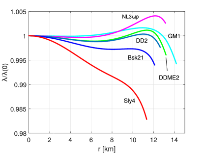
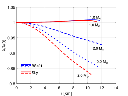
Figure 1: The relativistic factor $\lambda(r)$, normalised with respect to its value in the center $\lambda(0)$. In the upper panel we consider stars of $1.4\,M_{\odot}$ for six different equations of state: NL3$\omega\rho$ (without hyperons), GM1 (without hyperons), DDME2 (with hyperons), DD2 (without hyperons), BSk21 and Sly4 (Fortin et al., 2016; Fortin et al., 2017). In the lower panel we show the profile of $\lambda/\lambda(0)$ for different (Komar) masses for two selected equations of state: $M=1.0,\,2.0,\,2.2\,M_{\odot}$ for BSk21 (Goriely et al. 2010) and $M=1.0,\,2.0\,M_{\odot}$ for SLy4 (Douchin & Haensel 2001).

Consider the quantity $e^{\Phi-\Lambda}$, which we call first Ravenhall and Pethick (RP) parameter. Using the TOV equations, it is immediate to see that

$$\dfrac{d}{dr}\,e^{\Phi-\Lambda}=\dfrac{8}{3}\pi\,r\,e^{\Phi+\Lambda}\bigg{[}\braket{\mathcal{E}}_{2}-\dfrac{3}{2}(\mathcal{E}-\Psi)\bigg{]},$$ (102)

where $\braket{\mathcal{E}}_{2}$ is a volume average of the energy density,

$$\braket{\mathcal{E}}_{2}=\dfrac{3}{r^{3}}\int_{0}^{r}\,{r^{\prime}\,}^{2}\,\mathcal{E}(r^{\prime})\,dr^{\prime}.$$ (103)

The right-hand side of equation (102) goes to zero for $r=0$. However, there is a competition between $\braket{\mathcal{E}}_{2}$ and $(3/2)(\mathcal{E}-\Psi)$ for $r>0$. In the non-relativistic limit the pressure $\Psi$ is negligible with respect to $\mathcal{E}$, so that $3\mathcal{E}/2>\braket{\mathcal{E}}_{2}$ in the region extending from the center to the radius at which $e^{\Phi-\Lambda}$ reaches a minimum. The minimum, however, is reached not far from the surface for realistic equations of state, so that both $\braket{\mathcal{E}}_{2}$ and $3\mathcal{E}/2$ are small and $e^{\Phi-\Lambda}$ does not have the possibility to grow considerably. On the other hand, if the central pressure $\Psi(0)$ is comparable to the mass-energy density $\mathcal{E}(0)$, the inequality

$$\braket{\mathcal{E}}_{2}\,>\,3(\mathcal{E}-\Psi)/2$$ (104)

may hold also for small values of $r$; in this case $e^{\Phi-\Lambda}$ is an increasing function of the radial coordinate. Therefore, we have two extremal situations in which the first RP parameter is always respectively lower and higher with respect to its central values. As we can see in figure 2, neutron stars below their maximum mass are exactly on the turning point between these two different behaviors. So we happen to be in the situation in which

$$e^{\Phi-\Lambda}\approx const.$$ (105)

Figure 2 also shows that the error which we commit with this approximation is of the order of $10\%$.

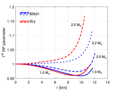
Figure 2: Plot of the first RP parameter, $e^{\Phi-\Lambda}$, normalised with its value in the center, for different (Komar) masses and equations of state: $M=1.0,\,2.0,\,2.2\,M_{\odot}$ for the BSk21 EOS (Goriely et al. (2010), blue curves) and $M=1.0,\,2.0\,M_{\odot}$ for the SLy EOS (Douchin & Haensel (2001), red curves).

Let us focus, now, on the quantity $j(1-\tilde{\omega})$, which we call second Ravenhall and Pethick parameter, where $j:=e^{-\Phi-\Lambda}$. Given the equation for the frame dragging of Hartle (1967), it is easy to see that

$$\dfrac{d}{dr}\,[j(1-\tilde{\omega})]=(1-\tilde{\omega})\dfrac{dj}{dr}-\langle\,(1-\tilde{\omega})\dfrac{dj}{dr}\,\rangle_{3}\,,$$ (106)

where

$$\langle\,(1-\tilde{\omega})\dfrac{dj}{dr}\,\rangle_{3}=\dfrac{4}{r^{4}}\int_{0}^{r}(1-\tilde{\omega}(r^{\prime}))\dfrac{dj}{dr^{\prime}}\,r^{\prime 3}dr^{\prime}\,.$$ (107)

Now, the TOV equations allow to verify that

$$(1-\tilde{\omega})\dfrac{dj}{dr}=-4\pi r(\mathcal{E}+\Psi)(1-\tilde{\omega})e^{-\Phi+\Lambda}.$$ (108)

For small $r$, both the terms in the right-hand side of equation (106) go to zero. As $r$ grows, $(1-\tilde{\omega})\partial_{r}j$ becomes negative, implying

$$(1-\tilde{\omega})\dfrac{dj}{dr}<\langle\,(1-\tilde{\omega})\dfrac{dj}{dr}\,\rangle_{3}\,.$$ (109)

This average gives more importance to the contributions close to $r$, implying that the difference $\partial_{r}j(1-\tilde{\omega})-\braket{\partial_{r}j(1-\tilde{\omega})}_{3}$ is small. As we move towards the surface of the star, the fact that $\mathcal{E}+\Psi$ goes to zero becomes increasingly important and lowers the value of $\partial_{r}j(1-\tilde{\omega})$, until we reach a point in which $(1-\tilde{\omega})\partial_{r}j=\braket{(1-\tilde{\omega})\partial_{r}j}_{3}$. Here we have the minimum of $j(1-\tilde{\omega})$ after which it will start growing. Thus, as can be seen in figure 3, we can conclude that

$$e^{-\Phi-\Lambda}(1-\tilde{\omega})\approx const$$ (110)

within an error of at most the $10\%$.

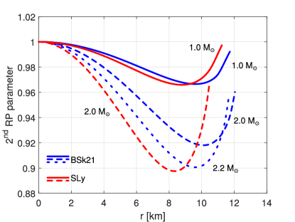
Figure 3: Plot of the second RP parameter, $e^{-\Phi-\Lambda}(1-\tilde{\omega})$, normalised with its value in the center, for different (Komar) masses and equations of state: $M=1.0,\,2.0,\,2.2\,M_{\odot}$ for the BSk21 EOS (Goriely et al. (2010), blue curves) and $M=1.0,\,2.0\,M_{\odot}$ for the SLy EOS (Douchin & Haensel (2001), red curves).

Since $\lambda$, apart from an overall constant factor, is the ratio of the two RP parameters, then it is approximately constant as well (within the $2\%$ for masses below 1.4 $M_{\odot}$ and the $17\%$ for masses close to the maximum mass, see figure 1). As a result, we do not present the plot of the vortex lines for the low mass cases because the relativistic effects are essentially invisible. We show only the profile for the most relativistic star considered here (i.e. a 2$M_{\odot}$ star with the SLy EOS, see figure 1). The result is shown in figure 4: the vortices are still essentially straight, as the gradients of $\mathcal{N}_{Newt}$ overwhelm the effect of the $\sim 20\%$ relativistic correction due to $\lambda$.

Finally, we remark that $\lambda\approx const$, which leads to almost straight vortex lines in this chart, is not the product of a more fundamental symmetry. Neutron stars supported by a realistic equation of state explore the particular range of parameters which guarantees this unexpected result. The use of unrealistic equations of state can lead to a highly deformed vortex structure. This is the case of Rothen (1981), who employed the equation of state $\mathcal{E}=const$, which is pathological, especially close to the maximum mass where $\Psi(0)\longrightarrow\infty$.

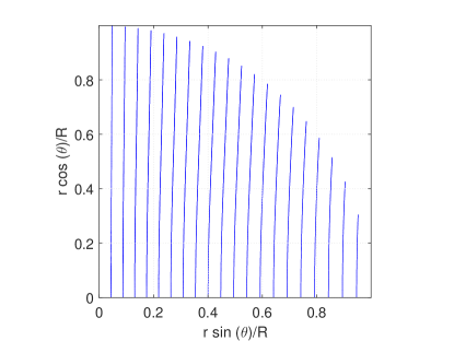
Figure 4: Vortex profile in the quasi-Schwarzschild coordinates for a neutron star of $2.0\,M_{\odot}$ described by the SLy EOS. The spacing between vortices has been chosen in a way to facilitate the visualization and does not reflect the vortex density.

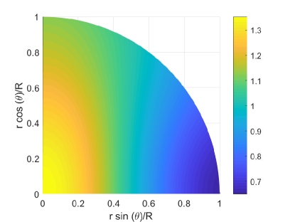
Figure 5: Map of $\mathfrak{N}_{Z}/\mathfrak{N}_{Newt}$ in the quasi-Schwarzschild coordinates, for a very compact neutron star of $2.0\,M_{\odot}$ described by the SLy EOS.

4.4 Approximate formula for the density of vortices

We now focus on the vortex density given by equation (98). In figure 5 we plot the density of vortices for a $2\,M_{\odot}$ neutron star governed by the Sly equation of state (Douchin & Haensel, 2001): it is higher close to the axis of symmetry, while has a minimum at the equator. Let us consider this behaviour in more detail.

When Ravenhall and Pethick’s approximation is applicable, we can put $\partial_{r}\lambda\approx 0$ in equation (98) to obtain

$$\mathfrak{N}_{Z}=\mathfrak{N}_{\textrm{Newt}}\lambda\sqrt{1+\sin^{2}\theta(-1+e^{-2\Lambda})}.$$ (111)

There is a simple geometrical interpretation for this result: the fact that $\lambda$ is nearly constant means that the vortices are perfectly vertical and uniformly distributed in the chart (this is analogous to the Newtonian case, since the only correction is given by the overall rescaling factor $\lambda$). However, when we have to compute the density $\mathfrak{N}_{Z}$ measured by the ZAMO, we need to consider also the fact that the lengths are distorted and that the density must be computed orthogonally to the vortex lines.

Consider two different ZAMOs, one on the polar axis and the other on the equatorial plane. In the first case the induced metric on the surface orthogonal to the vortices is

$$d\sigma^{2}=r^{2}d\theta^{2}+r^{2}\sin^{2}\theta d\varphi^{2},$$ (112)

which coincides with its Newtonian limit. Therefore, $\lambda$ is the only relativistic correction and

$$\mathfrak{N}_{Z}=\mathfrak{N}_{\textrm{Newt}}\,\lambda.$$ (113)

In the second case the surface element is

$$d\sigma^{2}=e^{2\Lambda}dr^{2}+r^{2}d\varphi^{2},$$ (114)

so that the space is dilated in the radial direction by a factor $e^{\Lambda}$ with respect to the Newtonian limit. As a consequence, the measure of surface density becomes

$$\mathfrak{N}_{Z}=\mathfrak{N}_{\textrm{Newt}}\,\lambda\,e^{-\Lambda}.$$ (115)

Therefore, the square root factor in (111) accounts for the fact that space is distorted: even if in the chart the vortices may be uniformly distributed (similarly to the Newtonian case), we still measure different local densities. The gravitational dilation of space in the radial direction is responsible for an alteration of the surface density, but only if the surface element has a radial extension, which explains the dependence on both $r$ and $\theta$ presented in equation (111).

In figure 6 we show the profile of the density of vortices on the equatorial plane for different solar masses, assuming the SLy equation of state. In the same figure, we also compare the exact formula (101) to the approximate one, (115). Clearly, the approximation is acceptable for low mass stellar configurations, but the induced error can be relevant for more massive stars. In all cases the approximation becomes better as we move towards the center, due to the fact that we are neglecting a term which is proportional to $r\partial_{r}\lambda$.

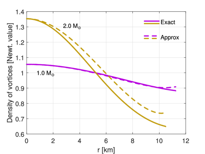
Figure 6: Plot of $\mathfrak{N}_{Z}/\mathfrak{N}_{Newt}$ as a function of $r$ along the equatorial plane ($\theta=\pi/2$), assuming the SLy equation of state. The continuous lines represent the exact surface density given by equation (98), the dashed ones represent the approximate result in equation (111).

5 Relativistic correction to the coupling time-scale

We are now ready to estimate the time-scale on which the mutual friction couples the superfluid and the normal components in a relativistic star. For a given velocity lag between the two components, we derive the time-scale on which the mutual friction couples them and re-establishes corotation. The time-scale we calculate is, therefore, also the one associated to the potentially observable spin-up phase in a pulsar glitch.

5.1 Small lag approximation

As a first step, we need to find the general expression for $\mu^{n}_{\varphi}$ in the presence of a velocity lag between the components. Given that $\Omega_{p}$ is uniform and represents the angular velocity of the neutron star we see from the Earth, let us consider the presence of a lag $\Omega_{np}:=\Omega_{n}-\Omega_{p}$ such that

$$\dfrac{|\Omega_{np}|}{\Omega_{p}}\ll 1,$$ (116)

so we can treat it as a perturbation. We also impose that the lag is different from zero only in a thin spherical shell (containing the crust), implying that the inertia of the part of superfluid which is not rotating with $\Omega_{p}$ is small compared to the rest of the star. This allows us to neglect the effect of this small lag on the metric.

The momentum per particle of the neutron superfluid can be written with the aid of an entrainment parameter $\epsilon_{n}$ (Prix et al., 2005) as

$$\mu_{\nu}^{n}=\mu_{n}^{(C)}\bigg{[}(1-\epsilon_{n})u_{n\nu}+\dfrac{\epsilon_{n}}{\Gamma_{np}}u_{p\nu}\bigg{]},$$ (117)

where $\mu_{n}^{(C)}$ is the comoving chemical potential (Gavassino & Antonelli, 2019). We have shown that, when the species corotate and are in chemical equilibrium, equation (88) holds. In the slow rotation approximation this condition can be rewritten as

$$\mu_{n}^{(C)}=m_{n}e^{\Phi_{D}-\Phi}.$$ (118)

This equation remains true also in the presence of a lag, provided that

$$\bigg{|}\Delta^{2}\dfrac{\partial\mu_{n}^{(C)}}{\partial\Delta^{2}}\bigg{|}_{n_{p},n_{n}}\bigg{|}\ll\mu_{n}^{(C)}.$$ (119)

It is easy to show that the above condition is equivalent to

$$|\epsilon_{n}|\Delta^{2}\ll 1,$$ (120)

which is verified in every realistic situation. Thus, we can plug equation (118) into equation (117) and use the slow-rotation approximation in (47), obtaining

$$\mu^{n}_{\varphi}=m_{n}e^{\Phi_{D}-2\Phi}\bigg{[}(1-\tilde{\omega})\Omega_{p}+(1-\epsilon_{n})\Omega_{np}\bigg{]}r^{2}\sin^{2}\theta.$$ (121)

Clearly, when $\Omega_{np}=0$ the above relation becomes equation (90).

We remark that if the lag was different from zero for every $r$, and not only in a thin shell of small moment of inertia, the frame dragging would be modified by the lag and would have the form $\omega=\tilde{\omega}\Omega_{p}+\omega^{\prime}$ where $\omega^{\prime}=\omega^{\prime}[\Omega_{np}]$ is a non-local linear functional of the lag. So in equation (121) a term $-\omega^{\prime}$ would appear inside the square brackets, which has the same order of $\Omega_{np}$ and therefore cannot be neglected. The consequences of this complication are discussed in section 6.

5.2 Local relaxation time

We compute here the timescale with which the velocity lag in different rings of constant $r$ and $\theta$ relax to corotation.

In the slow rotation approximation the relative velocity between the two components is

$$w_{np}=e^{-\Phi}\Omega_{np}\,\partial_{\varphi}.$$ (122)

Considering that $\hat{\perp}_{\varphi\varphi}\approx r^{2}\sin^{2}\theta$, the $\varphi$ component of equation (39) reads

$$\partial_{t}\mu_{\varphi}^{n}=-\dfrac{\mathcal{R}k\mathfrak{N}_{Z}}{1+\mathcal{R}^{2}}\Omega_{np}r^{2}\sin^{2}\theta.$$ (123)

Note that this equation coincides with equation (85) of Langlois et al. (1998), neglecting the convection angular velocity $\Omega_{+}$ and using the slow rotation approximation. Recalling equation (121), we find that

$$\partial_{t}\mu_{\varphi}^{n}=m_{n}e^{\Phi_{D}-2\Phi}[(1-\tilde{\omega})\dot{\Omega}_{p}+(1-\epsilon_{n})\partial_{t}\Omega_{np}]r^{2}\sin^{2}\theta.$$ (124)

Since the relaxation process we are considering is fast compared to the spin-down time-scale, the Komar angular momentum is approximately conserved. Moreover, we are assuming that the part of superfluid which is not locked to the normal component is contained in a thin shell of small moment of inertia. Therefore, the angular momentum conservation implies

$$|\dot{\Omega}_{p}|\ll|\partial_{t}\Omega_{np}|,$$ (125)

which allows us to neglect the term $(1-\tilde{\omega})\dot{\Omega}_{p}$ in (124). With the aid of this approximation, we can obtain from (123) a closed equation for the evolution of $\Omega_{np}$:

$$\partial_{t}\Omega_{np}=-\dfrac{\mathcal{R}k\mathfrak{N}_{Z}e^{2\Phi-\Phi_{D}}}{m_{n}(1+\mathcal{R}^{2})(1-\epsilon_{n})}\Omega_{np}.$$ (126)

Integrating this equation we obtain that for each ring of constant $r$ and $\theta$ we have a different relaxation time-scale,

$$t_{R,\textrm{GR}}^{(ring)}=\dfrac{m_{n}(1+\mathcal{R}^{2})(1-\epsilon_{n})}{\mathcal{R}k\mathfrak{N}_{Z}e^{2\Phi-\Phi_{D}}}.$$ (127)

Finally, isolating the Newtonian contribution

$$t_{R,\textrm{Newt}}^{(ring)}=\dfrac{m_{n}(1+\mathcal{R}^{2})(1-\epsilon_{n})}{\mathcal{R}k\mathfrak{N}_{\textrm{Newt}}},$$ (128)

we find, using (111) and (91),

$$t_{R,\textrm{GR}}^{(ring)}(r,\theta)=\dfrac{t_{R,\textrm{Newt}}^{(ring)}(r)}{(1-\tilde{\omega}(r))\sqrt{1+\sin^{2}\theta(-1+e^{-2\Lambda(r)})}}.$$ (129)

Hence, General Relativity introduces a dependence of the coupling time-scale on $\theta$ which is not present in the Newtonian limit. This is a direct consequence of the discussion in subsection 4.4.

It is important to remark that our formula for the time-scale has been derived under the fundamental assumption of a mutual friction which is proportional to the modulus of the macroscopic vorticity, see subsection 2.3. In a turbulent regime this assumption is likely to be violated and this might produce different contributions to the relativistic correction. To compute them, one can perform the same calculations we made in this subsection, modifying the right-hand side of (123) according to the alternative prescription for the mutual friction.

5.3 Global relaxation time

Different rings reach corotation on a different time-scale, but from the Earth we can observe only the changes of $\Omega_{p}$. Its evolution can be obtained by using angular momentum conservation, so its behaviour will not be a simple exponential but a weighted average of exponentials. We expect the average to favour those rings which are located around $\theta=\pi/2$ (the equatorial plane), as they are those with the largest moment of inertia. Therefore, employing also the fact that the metric functions vary slowly in the thin shell and can, thus, be evaluated at $r=R_{D}$, we obtain

$$\dfrac{t_{R,\textrm{GR}}}{t_{R,\textrm{Newt}}}=\dfrac{e^{\Lambda_{D}}}{1-\tilde{\omega}_{D}},$$ (130)

where $t_{R,\textrm{GR}}$ and $t_{R,\textrm{Newt}}$ are respectively the relativistic and the Newtonian prediction for the evolution of the angular velocity of the pulsar, seen from Earth.

We can now discuss the physical interpretation of equation (130) by taking into account all the expected relativistic effects:

• Gravitational time dilation: from Earth we observe a slow-motion picture of the internal dynamics of the star, thus the rise-time should be increased by a factor $e^{-\Phi_{D}}$. On the other hand, the time dilation increases the amount of vortices because an observer sitting inside the star sees faster motions. As the number of vortices increases, the mutual friction becomes stronger, so $t_{R,\textrm{GR}}$ is reduced by the factor $e^{\Phi_{D}}$. Thus the effects of time dilation cancel out.

• Curvature of space: in subsection 4.4 we have shown that the effect of gravity on the $t=const$ leaves is to enlarge the lengths in the radial direction. This reduces the density of vortices, increasing the rise-time by a factor $e^{\Lambda_{D}}$.

• Frame dragging: the frame-dragging constitutes a constant which needs to be subtracted to the angular velocity to connect what we observe from the Earth to what we would see if we were inside the star. Thus, it is not directly involved in the dynamical process. However it reduces the number of vortices, giving a factor $1-\tilde{\omega}_{D}$ in the denominator.

We can rewrite (130) in a more convenient way, considering that we can approximate the evaluation of the metric functions at the drip point with an evaluation at the surface of the star. In particular, given that

$$e^{\Lambda_{D}}\approx\bigg{(}1-\dfrac{2M}{R}\bigg{)}^{-1/2}\quad\quad\quad\tilde{\omega}_{D}\approx\dfrac{2I}{R^{3}},$$ (131)

where $M$ is the Komar mass and $I$ is the Hartle moment of inertia of the whole star, we arrive at

$$\dfrac{t_{R,\textrm{GR}}}{t_{R,\textrm{Newt}}}=\bigg{(}1-\dfrac{2M}{R}\bigg{)}^{-1/2}\bigg{(}1-\dfrac{2I}{R^{3}}\bigg{)}^{-1}.$$ (132)

This formula can be written only in terms of the relativistic compactness $\mathfrak{C}=M/R$ by using the universal relation

$$\dfrac{I}{R^{3}}=\bar{a}_{1}\mathfrak{C}^{2}+\bar{a}_{2}\mathfrak{C}+\bar{a}_{3}+\bar{a}_{4}\mathfrak{C}^{-1}\,,$$ (133)

where $\bar{a}_{1}=8.134\times 10^{-1}$, $\bar{a}_{2}=2.101\times 10^{-1}$, $\bar{a}_{3}=3.175\times 10^{-3}$ and $\bar{a}_{4}=-2.717\times 10^{-4}$ are coefficients which do not depend of the EOS (Breu & Rezzolla, 2016). Since all the formulas are given in geometric units, $\mathfrak{C}$, $I/R^{3}$ and the $\bar{a}_{i}$ are dimensionless.

In figure 7 we show the relativistic correction as a function of the compactness: the curve in the plot is practically independent from the equation of state used. We observe that the relativistic correction is always larger than 1 and for a typical star of 1.4 $M_{\odot}$ ($\mathfrak{C}\approx 0.18$) it is around $1.4$. This means that the coupling time-scale are always longer.

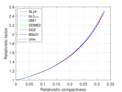
Figure 7: The relativistic factor $t_{R,\textrm{GR}}/t_{R,\textrm{Newt}}$ given in equation (132) as a function of the compactness $\mathfrak{C}$. For comparison purposes, we employed six different equations of state (Fortin et al., 2016; Fortin et al., 2017) to compute the moment of inertia $I=I(\mathfrak{C})$: all the curves appear to be nearly superimposed to the universal relation (133).

6 The role of the thin-shell assumption

In this final section we discuss why the thin-shell assumption is fundamental to find a universal formula for the relativistic correction to the mutual friction coupling time-scale.

An alternative approach to obtain a global correction is the one adopted by Sourie et al. (2017), where both the species are assumed to move rigidly. Differently from our approach (based on the presence of a thin shell that contains the superfluid neutrons), Sourie et al. (2017) focus on the relaxation process in the case in which the free superfluid component is extended over the whole core of the star. This introduces two complications. First, the quantities of interest are obtained as integrals over the star, loosing the universal character of equation (132) (which has been found by evaluating all the metric functions at the surface). Secondly, the frame dragging $\omega$ is a function of both $\Omega_{p}$ and $\Omega_{n}$, correcting the coefficient $1-\epsilon_{n}$ in equation (121) with a Lense-Thirring contribution (see the discussion in section 5). This is another effect which compromises the universality of the result, as it strongly depends on the details of internal stratification.

In this section we start from a rigid model and we impose the requirement that the density of the neutron superfluid, $n_{n}$, (which is formally extended over the whole core) is zero outside a thin shell located near the surface. We prove that under this assumption the formula for the relativistic correction to the coupling time-scale given by Sourie et al. (2017) reduces to (130), while in general it may differ from it.

6.1 Moments of inertia

Following Sourie et al. (2017) we have to introduce the partial moments of inertia of each species, because they appear directly in their formula for the correction to the coupling time-scale. As we said in subsection 5.1, in the thin shell limit the metric is essentially unaffected by the presence of the lag, implying that

$$\omega=\Omega_{p}\tilde{\omega}.$$ (134)

Using the slow rotation approximation, one can verify that the moment of inertia of the species $X$ defined in Sourie et al. (2017) is

$$\hat{I}_{X}=\int_{\Sigma}m_{n}n_{X}(1-\tilde{\omega})e^{\Lambda+\Phi_{D}-2\Phi}r^{2}\sin^{2}\theta\,d_{3}x,$$ (135)

where $\Sigma$ is a $t=const$ hypersurface, $d_{3}x=r^{2}\sin\theta\,dr\,d\theta\,d\varphi$, is the Newtonian volume element, and we have employed equation (118) to replace $\mu_{X}^{(C)}$. In the case $X=n$ the integrand is different from zero only in the thin shell, so the metric functions are approximately constant in the integral and can be replaced by their value on the drip point, thus we find

$$\hat{I}_{n}=(1-\tilde{\omega}_{D})e^{\Lambda_{D}-\Phi_{D}}\int_{\Sigma}m_{n}n_{n}r^{2}\sin^{2}\theta\,d_{3}x.$$ (136)

On the other hand, for $X=p$, the integral is extended over the whole star, so $\hat{I}_{p}\gg\hat{I}_{n}$. Defining $\hat{I}=\hat{I}_{p}+\hat{I}_{n}$, we have that

$$\hat{I}_{p}/\hat{I}\approx 1.$$ (137)

6.2 The gravitational space dilation factor

A second quantity which appears in the formula for the relativistic correction of Sourie et al. (2017) is the factor

$$\zeta:=\dfrac{1}{2\hat{I}_{n}\Omega_{n}}\int_{\Sigma}\Gamma_{nZ}\,n_{n}k\mathfrak{N}_{Z}\,{\perp}(\partial_{\varphi},\partial_{\varphi})e^{\Lambda}d_{3}x.$$ (138)

Using the slow rotation approximation, we have that

$$\Gamma_{nZ}\approx 1\quad\quad\quad{\perp}(\partial_{\varphi},\partial_{\varphi})\approx r^{2}\sin^{2}\theta.$$ (139)

Furthermore, since in the integral the angular part is weighed with a factor $\sin^{3}\theta$, we can replace $k\mathfrak{N}_{Z}$ with its value in $\theta=\pi/2$, which, using (115), reduces to

$$k\mathfrak{N}_{Z}=2m_{n}\Omega_{n}\lambda e^{-\Lambda}.$$ (140)

The thin shell approximation allows to replace all the metric functions in the integral with their value in $R_{D}$; recalling equation (91), we obtain

$$\zeta\approx e^{-\Lambda_{D}}.$$ (141)

Therefore $\zeta$ contains the correction to the density of vortices given by the gravitational dilation of space in the radial direction.

6.3 The generalised entrainment coefficients

In Sourie et al. (2017), the role of the entrainment and of the frame dragging on the coupling time-scale is encoded in two generalised entrainment coefficients $\hat{\epsilon}_{p}$ and $\hat{\epsilon}_{n}$. In this subsection we recap how they are defined and how they simplify under the thin-shell assumption.

Given and arbitrary function $f$, we introduce the two averaging procedures ($X=n,p$)

$$\braket{f}_{X}:=\dfrac{\int_{\Sigma}f\,m_{n}n_{X}e^{\Lambda+\Phi_{D}-2\Phi}r^{2}\sin^{2}\theta\,d_{3}x}{\int_{\Sigma}m_{n}n_{X}e^{\Lambda+\Phi_{D}-2\Phi}r^{2}\sin^{2}\theta\,d_{3}x}.$$ (142)

In particular, Sourie et al. (2017) define

$$\tilde{\epsilon}_{X}=\braket{\epsilon_{X}}_{X}.$$ (143)

It is clear that $\epsilon_{p}=0$ outside the superfluid domain. Since the denominator (an integral over the whole star) is much larger than the numerator (restricted over the thin shell), we have that

$$\tilde{\epsilon}_{p}\approx 0\,.$$ (144)

The authors also average the frame dragging and split the contributions as

$$\braket{\omega}_{X}=\epsilon^{LT}_{XX}\Omega_{X}+\epsilon^{LT}_{YX}\Omega_{Y}.$$ (145)

Using the approximation (134), it is clear that

$$\epsilon^{LT}_{nn}\approx\epsilon^{LT}_{np}\approx 0\quad\quad\quad\epsilon^{LT}_{pn}\approx\tilde{\omega}_{D}.$$ (146)

Finally they define the coefficients

$$\hat{\epsilon}_{X}=\dfrac{\tilde{\epsilon}_{X}-\epsilon^{LT}_{YX}}{1-\epsilon^{LT}_{XX}-\epsilon^{LT}_{YX}},$$ (147)

which, considering (144) and (146), become

$$\hat{\epsilon}_{p}\approx 0\quad\quad\quad\hat{\epsilon}_{n}\approx\dfrac{\tilde{\epsilon}_{n}-\tilde{\omega}_{D}}{1-\tilde{\omega}_{D}}.$$ (148)

6.4 Relativistic correction to the rise time

Now we have all the ingredients we need to study the relativistic correction to the rise time of Sourie et al. (2017),

$$\dfrac{t_{R,\textrm{GR}}}{t_{R,\textrm{Newt}}}=\dfrac{\hat{I}_{p}^{\textrm{GR}}/\hat{I}^{\textrm{GR}}}{\hat{I}_{p}^{\textrm{Newt}}/\hat{I}^{\textrm{Newt}}}\cdot\dfrac{1-\hat{\epsilon}_{p}^{\textrm{GR}}-\hat{\epsilon}_{n}^{\textrm{GR}}}{1-\tilde{\epsilon}_{p}^{\textrm{Newt}}-\tilde{\epsilon}_{n}^{\textrm{Newt}}}\cdot\zeta^{-1}\,,$$ (149)

in the thin-shell approximation.

Noting that equations (137) and (144) are true both in Newtonian theory and in General Relativity, we can use (141) and (148) to obtain

$$\dfrac{t_{R,\textrm{GR}}}{t_{R,\textrm{Newt}}}=\dfrac{1-\tilde{\epsilon}_{n}^{\textrm{GR}}}{1-\tilde{\epsilon}_{n}^{\textrm{Newt}}}\cdot\dfrac{e^{\Lambda_{D}}}{1-\tilde{\omega}_{D}}\,.$$ (150)

However, $\tilde{\epsilon}_{n}^{GR}\approx\tilde{\epsilon}_{n}^{\textrm{Newt}}$, because the relativistic corrections (given by the metric functions) can be brought out of the average over the thin shell, canceling out. Thus, we finally arrive at

$$\dfrac{t_{R,\textrm{GR}}}{t_{R,\textrm{Newt}}}=\dfrac{e^{\Lambda_{D}}}{1-\tilde{\omega}_{D}}\,,$$ (151)

which is what we wanted to prove.

If the thin shell approximation is not valid, however, (137), (144) and (151) do not hold and the relativistic correction will depend on the EOS as is seen in figure 8 of Sourie et al. (2017).

To date, there is no general consensus on the real extension of the superfluid region involved in the rise of a glitch. The standard scenario of a pinned superfluid confined only in the inner crust has been challenged in Andersson et al. (2012), Chamel (2013) and Pizzochero et al. (2019). An extension of the region including only an external fraction of the core for young neutron stars has been proposed by Ho et al. (2015). This model remains in the limit of the thin shell assumption. On the other hand, Gügercinoğlu & Alpar (2014) have proposed that the whole core may contribute to the glitch, which would imply the need of employing the scheme adopted by Sourie et al. (2017).

7 Conclusions

We have computed the relativistic correction to the coupling time-scale between the superfluid and the normal component in a neutron star.

In doing this, we analysed all the quantities involved in the mutual friction equation. First, we studied the vortex profile in general relativity, verifying that the formula presented in Rothen (1981) can be easily justified directly from Carter’s two-fluid formalism in the slow rotation approximation. Secondly, we found that the validity of the approximations presented in Ravenhall & Pethick (1994) implies that the vortex lines are expected to be almost straight in the quasi-Schwarzschild coordinates. Furthermore, we derived a formula for the vortex density, which, making use of the approximations of Ravenhall & Pethick (1994), becomes proportional to a geometric factor encoding the gravitational dilation of space in the radial direction.

Inserting all the results in the prescription for the vortex-mediated mutual friction presented in Langlois et al. (1998) we have shown that the relativistic corrections to the coupling time-scale are given, in the crust and in the outermost part of the outer core, by a universal factor which is a function of the compactness of the star only. This universal correction incorporates the effects of space curvature, which dilates the vortex spacing, and of the frame dragging, which reduces the amount of vortices. Both these effect reduce the mutual friction between the two species, slowing down the coupling process. For a typical star of 1.4 $M_{\odot}$ the glitch rise-time is enhanced of the $40\%$ with respect to Newtonian predictions. The correction grows as the star becomes more compact (and thus relativistic).

Currently, Newtonian models are mostly employed to fit glitch rise-times and extract constraints on the mutual friction coefficients (Haskell et al., 2018; Ashton et al., 2019; Pizzochero et al., 2019), with the notable exception of (Sourie et al., 2017), who however consider the superfluid reservoir to be in the core of the star. In the case in which the reservoir is assumed to be in the crust, the mutual friction coefficients obtained by means of Newtonian models should just be rescaled with the coefficient given in equation (132) to encode the corrections of General Relativity. This result is particularly useful because the factor is a universal function of the compactness and, therefore, does not depend on the equation of state. We remark that Ho et al. (2015) and Newton et al. (2015) propose techniques to distinguish equations of state based on differences that have the same order of magnitude as the relativistic correction that we obtain. Thus in these studies the effect of General Relativity cannot be neglected and our prescription for the correction needs to be adopted.

The general picture emerging from the present paper is that, despite the intrinsic difficulties of a fully relativistic approach, in the quasi-Schwarzschild coordinates all the relativistic effects assume a simple and intuitive form. The factors $e^{\Phi}$ (encoding gravitational time dilation), $e^{\Lambda}$ (encoding the curvature of space) and $\tilde{\omega}$ (encoding the Lense-Thirring effect) always appear in positions which are coherent with their intuitive meaning and their presence could also be deduced by means of simple arguments (see subsections 4.2, 4.4 and 5.3).

Finally, the present work (together with similar ones, see e.g. Langlois et al. (1998), Andersson & Comer (2001), Sourie et al. (2017) and Antonelli et al. (2018)) can be used as a theoretical basis for the development of refined relativistic dynamical models for pulsar glitches and neutron star oscillations in the framework of the slow rotation approximation.

Appendix A Trough the eyes of an ideal observer

Let us consider an ideal observer $\mathcal{O}$ with a four-velocity $u_{\mathcal{O}}$. We define the pseudovorticity associated to $\mathcal{O}$ as

$$\varpi_{\mathcal{O}}^{\nu}:=-{\star}\varpi^{\nu\rho}\,u_{\mathcal{O}\rho}=\varpi\,\mathcal{S}^{\nu\rho}u_{\mathcal{O}\rho}.$$ (152)

Considering the antisymmetry of ${\star}\varpi^{\nu\rho}$, it is evident that

$$\varpi_{\mathcal{O}}^{\nu}u\indices{{}_{\mathcal{O}\nu}}=0,$$ (153)

so that in the local reference frame of the observer it is a spatial vector. Equation (21) immediately gives

$${\perp}\indices{{}^{\nu}_{\rho}}\varpi_{\mathcal{O}}^{\rho}=0,$$ (154)

which tells us that the pseudovorticity is tangent to the wordlsheet. Hence, $\varpi_{\mathcal{O}}$ points along the intersection between the vortex worldsheet and the local set of simultaneous events of the observer (this intersection is just the profile of the vortex locally seen by $\mathcal{O}$). Furthermore, we define

$$v_{\mathcal{O}}:=\dfrac{\varpi_{\mathcal{O}}}{\sqrt{g(\varpi_{\mathcal{O}},\varpi_{\mathcal{O}})}},$$ (155)

which is the unit vector which points along the vorticity lines seen by the observer. Using (22), it is easy to show that the denominator in the definition (155) can be rewritten as

$$\sqrt{g(\varpi_{\mathcal{O}},\varpi_{\mathcal{O}})}=\varpi\sqrt{-g(\mathbin{\,\!/\mkern-5.0mu/\!}\,u_{\mathcal{O}},\mathbin{\,\!/\mkern-5.0mu/\!}\,u_{\mathcal{O}})}.$$ (156)

Another useful vector is

$$u_{{V\mathcal{O}}}:=\dfrac{\mathbin{\,\!/\mkern-5.0mu/\!}\,u_{\mathcal{O}}}{\sqrt{-g(\mathbin{\,\!/\mkern-5.0mu/\!}\,u_{\mathcal{O}},\mathbin{\,\!/\mkern-5.0mu/\!}\,u_{\mathcal{O}})}},$$ (157)

which we refer to as vortex four-velocity (with respect to the observer $\mathcal{O}$). Equations (22) and (156) can be used to verify that

$$u_{V{\mathcal{O}}}^{\nu}=\mathcal{S}^{\nu\rho}v_{{\mathcal{O}}\rho},$$ (158)

implying

$$u_{V{\mathcal{O}}}^{\nu}v\indices{{}_{\mathcal{O}}{}_{\nu}}=0.$$ (159)

To understand the meaning of $u_{V{\mathcal{O}}}$, imagine to mark a point in the core of a vortex. The worldline of this point is contained into the wordsheet of the corresponding vortex, implying that its four-velocity will be tangent to it. Clearly, there are infinitely many ways this particle can slide along the vortex line and this is reflected in the fact that the kernel of $\varpi_{\nu\rho}$ is a two-dimensional plane containing several normalised future-oriented timelike four-vectors $u_{C}$. In general, these $u_{C}$ are solutions of (29) and can be written as

$$u_{C}(\zeta):=u_{V{\mathcal{O}}}\cosh(\zeta)+v_{\mathcal{O}}\sinh(\zeta).$$ (160)

Let us impose that the marked point is moving with four-velocity $u_{V{\mathcal{O}}}$, which is the case $\zeta=0$. Then,

$$\Gamma_{V{\mathcal{O}}}:=-g(u_{\mathcal{O}},u_{V{\mathcal{O}}})=\sqrt{-g(\mathbin{\,\!/\mkern-5.0mu/\!}\,u_{\mathcal{O}},\mathbin{\,\!/\mkern-5.0mu/\!}\,u_{\mathcal{O}})}$$ (161)

is the Lorentz factor associated with its relative speed with respect to $O$, while the vector

$$w_{V{\mathcal{O}}}:=\dfrac{u_{V{\mathcal{O}}}}{\Gamma_{V{\mathcal{O}}}}-u_{\mathcal{O}},$$ (162)

represents the three-velocity of the particle seen by the observer. Moreover $w_{V{\mathcal{O}}}$ is orthogonal (making use of (153) and (159)) to $v_{\mathcal{O}}$. This means that $u_{V{\mathcal{O}}}$ represents the four-velocity that the matter contained in the core of the vortices would have if we suppose that in the frame of $\mathcal{O}$ its motion is perpendicular to the shape of the vortices. For this reason, it can be considered to be the four-velocity of the vortices with respect to $\mathcal{O}$, as it describes how their profile moves in their local frame. In particular, it is easy to show that

$$\Gamma_{V{\mathcal{O}}}=\dfrac{1}{\sqrt{1-\Delta_{V{\mathcal{O}}}^{2}}}\quad\quad\quad\Delta_{V{\mathcal{O}}}^{2}=g(w_{V{\mathcal{O}}},w_{V{\mathcal{O}}}).$$ (163)

We now derive the local density of vortices measured by the observer. To do so, it is necessary to use the Feynman-Onsager quantization condition which emerges from (13), see also Antonelli et al. (2018). Consider a spacelike two-dimensional surface $\Sigma$ in the superfluid domain, enclosed by a circuit $\partial\Sigma$. It is immediate to see that

$$\int_{\partial\Sigma}\mu=k\mathcal{N},$$ (164)

where $\mathcal{N}$ is the net number of vortices enclosed by $\partial\Sigma$ (Antonelli et al., 2018). Employing Stokes’ theorem and the fact that the exterior derivative commutes with the pull-back,

$$\mathcal{N}=\dfrac{1}{k}\int_{\Sigma}\varpi.$$ (165)

Let us define at each point of $\Sigma$ an orthonormal basis $e_{a}$, such that $e_{0}$ (time-like) and $e_{1}$ are normal to it, while $e_{2}$ and $e_{3}$ are tangent. In the text we employ the convention that, in the integral, the pull-back of $\varpi$ is identified with $\varpi$ itself. Since, however, the pull-back of $\varpi$ is a 2-form defined in a two-dimensional space, then

$$\int_{\Sigma}\varpi=\int_{\Sigma}\varpi(e_{2},e_{3})\sqrt{G}\,d_{2}x,$$ (166)

where $\sqrt{G}$ is the square root of the determinant of the metric induced on $\Sigma$. Considering the fact that in a Lorentzian manifold the Hodge dual has the property

$${\star}{\star}=-1$$ (167)

on two-forms, we can write

$$\varpi(e_{2},e_{3})=\varpi_{23}=-\varepsilon_{0123}{\star}\varpi^{01}={\star}\varpi(e_{0},e_{1}).$$ (168)

Defining the unit bivector normal to the surface

$$\mathcal{S}^{\nu\rho}_{\Sigma}:=e_{0}^{\nu}e_{1}^{\rho}-e_{0}^{\rho}e_{1}^{\nu},$$ (169)

it is evident that

$${\star}\varpi(e_{0},e_{1})=\dfrac{1}{2}{\star}\varpi_{\nu\rho}\mathcal{S}^{\nu\rho}_{\Sigma}\,.$$ (170)

Plugging our result into the integral we finally obtain

$$\mathcal{N}=\dfrac{1}{2k}\int_{\Sigma}{\star}\varpi_{\nu\rho}d\Sigma^{\nu\rho},$$ (171)

where we used the compact notation

$$d\Sigma^{\nu\rho}:=\mathcal{S}^{\nu\rho}_{\Sigma}d\Sigma\quad\quad\quad\text{with}\quad\quad\quad d\Sigma:=\sqrt{G}\,d_{2}x.$$ (172)

Therefore, the integral of the two-form has been transformed into the flux of its Hodge dual. Defined the scalar

$$\mathfrak{N}:=\dfrac{\varpi}{k},$$ (173)

we are able to write

$$\mathcal{N}=-\dfrac{1}{2}\int_{\Sigma}\mathfrak{N}\mathcal{S}_{\nu\rho}d\Sigma^{\nu\rho}.$$ (174)

The density of vortices is a number per unit area and must be computed by considering surfaces which are orthogonal to the profile of the vortices. Thus, to obtain the local density of vortices $\mathfrak{N}_{\mathcal{O}}$ measured by $\mathcal{O}$, we need to consider an infinitesimal area $\delta S$ that is orthogonal to both $u_{\mathcal{O}}$ and $v_{\mathcal{O}}$. This gives

$$\mathcal{S}^{\nu\rho}_{\Sigma}=u_{\mathcal{O}}^{\nu}v_{\mathcal{O}}^{\rho}-u_{\mathcal{O}}^{\rho}v_{\mathcal{O}}^{\nu}$$ (175)

and using (157), (158) and (161), we arrive at

$$\mathfrak{N}_{\mathcal{O}}=\dfrac{\mathcal{N}}{\delta\Sigma}=-\mathfrak{N}\mathcal{S}^{\nu\rho}u_{{\mathcal{O}}\nu}v_{{\mathcal{O}}\rho}=\mathfrak{N}\Gamma_{V{\mathcal{O}}}.$$ (176)

Looking again at equation (155) and (156), we notice that the norm of $\varpi_{\mathcal{O}}$ is the density measured by $O$ (apart from the factor $k$). Hence, the pseudovorticity can be written as

$$\varpi_{\mathcal{O}}=k\mathfrak{N}_{\mathcal{O}}v_{\mathcal{O}}.$$ (177)

Notice that if the four-velocity is tangent to the wordsheet (meaning that for the relative observer the vortices are locally at rest), the density of vortices $\mathfrak{N}_{\mathcal{O}}$ reduces to $\mathfrak{N}$. This tells us that $\mathfrak{N}$ can be considered to be the rest-frame vortex density. Now the formula (27) has a clear interpretation: the factor $\Gamma_{V{\mathcal{O}}}$ encodes the contraction of lengths, which modifies the densities only if the velocity of the observer has a component which is orthogonal to the vortex profile.

Appendix B Relativistic mutual friction

Let us start by rearranging the terms of (38) as

$$(g_{\nu\rho}-\mathcal{R}^{-1}\Gamma_{vp}^{-1}\varepsilon_{\nu\mu\rho\sigma}u_{n}^{\mu}v_{p}^{\sigma})u_{v}^{\rho}=\Gamma_{vp}^{-1}u_{p\nu}.$$ (178)

This relation defines $u_{v}$ in terms of $u_{p}$, $v_{p}$ and $u_{n}$: we can solve it for $u_{v}$, considering now $\Gamma_{vp}$ as a parameter and ignoring for the moment the fact that it is a function of $u_{v}$ itself. To simplify the calculations we choose a convenient orthonormal basis $e_{a}=e_{a}^{\mu}\partial_{\mu}$ such that $e_{0}=u_{n}$ and $v_{p}\in span\{e_{0},e_{1}\}$, with $v_{p}^{1}>0$. In this tetrad equation (178) reads

$$\mathcal{M}_{ab}u_{v}^{b}=\Gamma_{vp}^{-1}u_{pa},$$ (179)

where

$$\mathcal{M}_{ab}=\eta_{ab}+\mathcal{Z}\,\varepsilon_{01ab}\quad\quad\quad\mathcal{Z}=\mathcal{R}^{-1}\Gamma_{vp}^{-1}v_{p}^{1},$$ (180)

whose matrix representation on this basis is

$$\mathcal{M}_{ab}=\begin{bmatrix}-1&0&0&0\\ 0&1&0&0\\ 0&0&1&\mathcal{Z}\\ 0&0&-\mathcal{Z}&1\end{bmatrix}.$$ (181)

Now, if we are able to find the tensor $\mathcal{M}^{ca}_{(inv)}$ such that

$$\mathcal{M}^{ca}_{(inv)}\mathcal{M}_{ab}=\delta\indices{{}^{c}_{b}},$$ (182)

then contracting (179) with $\mathcal{M}^{ca}_{(inv)}$ gives

$$u_{v}^{c}=\mathcal{M}_{(inv)}^{ca}\Gamma_{vp}^{-1}u_{pa},$$ (183)

which is the expression we are looking for. Since the matrix form of $\mathcal{M}_{(inv)}$ is the inverse of $\mathcal{M}$, it is now clear why the choice of this basis is so convenient: in fact, it is easy to invert (181), namely

$$\mathcal{M}^{ca}_{(inv)}=\begin{bmatrix}-1&0&0&0\\ 0&1&0&0\\ 0&0&\dfrac{1}{1+\mathcal{Z}^{2}}&-\dfrac{\mathcal{Z}}{1+\mathcal{Z}^{2}}\\ 0&0&\dfrac{\mathcal{Z}}{1+\mathcal{Z}^{2}}&\dfrac{1}{1+\mathcal{Z}^{2}}\end{bmatrix},$$ (184)

which in a tensorial notation can be written as

$$\mathcal{M}_{(inv)}^{ca}=\eta^{ca}-\dfrac{\mathcal{Z}}{1+\mathcal{Z}^{2}}\varepsilon\indices{{}_{0}{}_{1}^{c}{}^{a}}-\dfrac{\mathcal{Z}^{2}}{1+\mathcal{Z}^{2}}\hat{\perp}^{ca},$$ (185)

where $\hat{\perp}\indices{{}^{\nu}_{\rho}}$ is the projector onto the plane generated by $e_{2}$ and $e_{3}$.

We use (185) into (183), lower the index $c$ and rewrite everything in a generic coordinate basis, obtaining

$$u_{v\nu}=\dfrac{u_{p\nu}}{\Gamma_{vp}}-\dfrac{\mathcal{R}^{-1}}{1+\mathcal{Z}^{2}}u_{n}^{\lambda}v_{p}^{\sigma}\varepsilon_{\lambda\sigma\nu\rho}\dfrac{u_{p}^{\rho}}{\Gamma_{vp}^{2}}-\dfrac{\mathcal{Z}^{2}}{1+\mathcal{Z}^{2}}\hat{\perp}_{\nu\rho}\dfrac{u_{p}^{\rho}}{\Gamma_{vp}}.$$ (186)

This equation is an exact reformulation of (37). In our model, however, we will work in the limit in which the relative speeds between all the species are non relativistic, so we can neglect the Lorentz factors and consider the limit

$$\mathcal{Z}\longrightarrow\dfrac{1}{\mathcal{R}}.$$ (187)

It is, also, useful to introduce the relative three-velocities, defined in general by the condition

$$u_{x}=:\Gamma_{xy}(u_{y}+w_{xy}),$$ (188)

which in this limit become

$$w_{xy}=u_{x}-u_{y}.$$ (189)

Equation (186), then, reduces to

$$w_{vp\nu}=\dfrac{\mathcal{R}}{1+\mathcal{R}^{2}}u_{n}^{\lambda}v_{p}^{\sigma}\varepsilon_{\lambda\sigma\nu\rho}w_{np}^{\rho}+\dfrac{\hat{\perp}_{\nu\rho}w_{np}^{\rho}}{1+\mathcal{R}^{2}}.$$ (190)

Consider again equation (37); in the limit of small relative speeds

$${\perp}u_{p}\approx-w_{vp}$$ (191)

and we can rewrite the right-hand side employing (190), arriving at

$$-u_{n}^{\rho}\varpi^{n}_{\rho\nu}=\dfrac{\mathcal{R}k\mathfrak{N}}{1+\mathcal{R}^{2}}\bigg{[}\mathcal{R}u_{n}^{\lambda}v_{p}^{\sigma}\varepsilon_{\lambda\sigma\nu\rho}w_{np}^{\rho}+\hat{\perp}_{\nu\rho}w_{np}^{\rho}\bigg{]},$$ (192)

which is the expression of mutual friction we were looking for (see Andersson et al. 2016 for an alternative derivation).

Appendix C Closed degenerate two-forms in General Relativity

In this appendix we briefly review the geometrical properties of two-forms in General Relativity, expanding some concepts that have been touched in section 2.2. In particular, we show that the degeneracy condition (15) is sufficient to guarantee the existence of a two-dimensional foliation whose leaves are tangent to the kernel of the two-form. In the following, the names of the tensors which we introduce are those of the fields of electrodynamics in General Relativity. This because the formalism we are going to build is employed exactly as presented here also in GRMHD (Gourgoulhon, 2013; Gralla & Jacobson, 2014).

Consider an arbitrary two-form $F$. Given the four-velocity $u_{\mathcal{O}}$ of an observer, we can build a right-handed orthonormal basis $e_{a}=e_{a}^{\mu}\partial_{\mu}$ such that $e_{0}=u_{\mathcal{O}}$. The form $F$ can be expanded in this basis as

$$F=\dfrac{1}{2}F_{ab}\,e^{a}\wedge e^{b}$$ (193)

and the components $F_{ab}$ represent what is measured by the observer moving with $u_{\mathcal{O}}$. In this basis we can rename the components of $F_{ab}$ according to the Faraday decomposition

$$F_{ab}=\begin{bmatrix}0&-E_{1}&-E_{2}&-E_{3}\\ E_{1}&0&B_{3}&-B_{2}\\ E_{2}&-B_{3}&0&B_{1}\\ E_{3}&B_{2}&-B_{1}&0\end{bmatrix}.$$ (194)

We can introduce the two covectors

$$E_{\mathcal{O}}:=E_{j}e^{j}\quad\quad\quad B_{\mathcal{O}}:=B_{j}e^{j},$$ (195)

where $j$ runs from $1$ to $3$ and we put the subscript ${\mathcal{O}}$ to keep track of the fact that everything depends on the choice of the observer. Using the musical duality notation

$$u_{\mathcal{O}}^{\flat}:=u_{{\mathcal{O}}\nu}dx^{\nu},$$ (196)

$F$ can be rewritten as

$$F=u_{\mathcal{O}}^{\flat}\wedge E_{\mathcal{O}}+\star(u_{\mathcal{O}}^{\flat}\wedge B_{\mathcal{O}}).$$ (197)

Moreover,

$$(\star F)_{ab}=\begin{bmatrix}0&B_{1}&B_{2}&B_{3}\\ -B_{1}&0&E_{3}&-E_{2}\\ -B_{2}&-E_{3}&0&E_{1}\\ -B_{3}&E_{2}&-E_{1}&0\end{bmatrix},$$ (198)

which can be seen as the result of the transformation

$$E_{\mathcal{O}}\rightarrow-B_{\mathcal{O}}\quad\quad\quad B_{\mathcal{O}}\rightarrow E_{\mathcal{O}}$$ (199)

and implying that

$$\star F=-u_{\mathcal{O}}^{\flat}\wedge B_{\mathcal{O}}+\star(u_{\mathcal{O}}^{\flat}\wedge E_{\mathcal{O}}).$$ (200)

The properties of the wedge product and of the Hodge duality, together with equations (197) and (200), can be used to prove that

$$E_{\mathcal{O}}=-\iota_{u_{\mathcal{O}}}F\quad\quad\quad\quad\quad\quad B_{\mathcal{O}}=\iota_{u_{\mathcal{O}}}{\star}F.$$ (201)

Thus we have a simple way to extract, for a given $F$ and $u_{\mathcal{O}}$, the two covectors $E_{\mathcal{O}}$ and $B_{\mathcal{O}}$. Notice also that $E_{\mathcal{O}}$ and $B_{\mathcal{O}}$ can be combined to give two scalars which do not depend on the choice of $u_{\mathcal{O}}$. In fact, it is immediate to verify that

$$\begin{split}&\braket{F,F}=\braket{B_{\mathcal{O}},B_{\mathcal{O}}}-\braket{E_{\mathcal{O}},E_{\mathcal{O}}}\\ &\braket{F,{\star}F}=2\braket{E_{\mathcal{O}},B_{\mathcal{O}}},\end{split}$$ (202)

where $\braket{,}$ is the inner product of forms. Now, let us suppose there is a four-velocity field $u_{C}$ such that

$$\iota_{u_{C}}F=0$$ (203)

everywhere. According to (201) this is equivalent to requiring that in every point of the spacetime the quantity $E$ associated to $u_{C}$ is equal to zero. We call (employing again the musical duality formalism)

$$\mathbb{B}:=(\iota_{u_{C}}{\star}F)^{\#},$$ (204)

which is the $B$ associated to $u_{C}$ with raised indices. Hence, from (197), we immediately have that

$$F=\star(u_{C}^{\flat}\wedge\mathbb{B}^{\flat}).$$ (205)

Now in every point of the spacetime we can consider the plane $\mathcal{K}:=span\{u_{C},\mathbb{B}\}$. This two-dimensional plane coincides with the kernel of $F$, i.e. it is the set of all the vectors $v$ such that $\iota_{v}F=0$. According to Frobenius’ theorem, the condition for the existence of a regular foliation of the spacetime in two-dimensional worldsheets which are in every point tangent to the corresponding $\mathcal{K}$ is that for any couple of vector fields $X$ and $Y$ which take values in $\mathcal{K}$ everywhere, their commutator takes values in $\mathcal{K}$ itself. However, from

$$\iota_{[X,Y]}F=[\mathcal{L}_{X},\iota_{Y}]F,$$ (206)

and using Cartan’s magic formula and the conditions $\iota_{X}F=\iota_{Y}F=0$, one finds that the condition for the hypotheses of the Frobenius theorem to hold is that

$$\iota_{X}\iota_{Y}dF=0,$$ (207)

for all $X$, $Y$ in $\mathcal{K}$. In particular, if $dF=0$, the existence of the foliation is guaranteed.

In the electromagnetic setting $F=dA$, so $dF=d^{2}A=0$ and the degeneracy condition is verified in the case of force-free GRMHD (Gralla & Jacobson, 2014). The worldsheet foliation, then, describes evolution of the magnetic-field lines.

As a last remark, note that equation (203) automatically implies, according to (202), that

$$\braket{F,{\star}F}=0,$$ (208)

which is equivalent to

$$F\wedge F=0.$$ (209)

C.1 $E\times B$ drift velocity

Consider a closed and degenerate two-form $F$ which can be written in the form presented in equation (205). Then, for a given observer with four-velocity $u_{\mathcal{O}}$ it is possible to define the quantity

$$w_{E\times B}^{\mathcal{O}}:=\dfrac{\star(u_{\mathcal{O}}\wedge E_{\mathcal{O}}\wedge B_{\mathcal{O}})}{\braket{B_{\mathcal{O}},B_{\mathcal{O}}}}.$$ (210)

In the frame of the observer this four-vector takes the form

$${w_{E\times B}^{\mathcal{O}}}^{j}=\dfrac{(E_{\mathcal{O}}\times B_{\mathcal{O}})^{j}}{|B_{\mathcal{O}}|^{2}}.$$ (211)

If $F$ is the Faraday tensor, so we can interpret $E_{\mathcal{O}}$ and $B_{\mathcal{O}}$ as respectively the electric and magnetic fields in the frame of $\mathcal{O}$, then $w_{E\times B}^{\mathcal{O}}$ is the so called $E\times B$ drift velocity (Bellan, 2006).

Let us write $w_{E\times B}^{\mathcal{O}}$ in terms of $u_{C}$, $\mathbb{B}$ and $u_{\mathcal{O}}$. It is convenient to work in components; combining (201) and (205), we find that

$$\begin{split}&E_{\mathcal{O}\mu}=\varepsilon_{\mu\nu\rho\sigma}u_{\mathcal{O}}^{\nu}u_{C}^{\rho}\mathbb{B}^{\sigma}\\ &B_{\mathcal{O}\mu}=\Gamma_{\mathcal{O}C}\mathbb{B}_{\mu}+g(u_{\mathcal{O}},\mathbb{B})u_{C\mu},\end{split}$$ (212)

which immediately implies

$$\braket{B_{\mathcal{O}},B_{\mathcal{O}}}=g(\mathbb{B},\mathbb{B})\Gamma_{\mathcal{O}C}^{2}-g(u_{\mathcal{O}},\mathbb{B})^{2}.$$ (213)

By definition, the numerator of the right-hand side of equation (210) is, in components,

$$\star(u_{\mathcal{O}}\wedge E_{\mathcal{O}}\wedge B_{\mathcal{O}})^{\mu}=\varepsilon^{\nu\rho\sigma\mu}u_{\mathcal{O}\nu}E_{\mathcal{O}\rho}B_{\mathcal{O}\sigma}.$$ (214)

Plugging equations (212) inside this identity, and using the condition

$$\varepsilon^{\lambda\nu_{1}\nu_{2}\nu_{3}}\varepsilon_{\lambda\rho_{1}\rho_{2}\rho_{3}}=-3!\delta\indices{{}^{[\nu_{1}}_{\rho_{1}}}\delta\indices{{}^{\nu_{2}}_{\rho_{2}}}\delta\indices{{}^{\nu_{3}]}_{\rho_{3}}},$$ (215)

it is possible to verify that

$$\begin{split}\star(u_{\mathcal{O}}\wedge E_{\mathcal{O}}\wedge B_{\mathcal{O}})^{\mu}=&g(\mathbb{B},\mathbb{B})\Gamma_{\mathcal{O}C}u_{C}^{\mu}+g(u_{\mathcal{O}},\mathbb{B})\mathbb{B}^{\mu}\\ &-[\Gamma_{\mathcal{OC}}^{2}g(\mathbb{B},\mathbb{B})-g(u_{\mathcal{O}},\mathbb{B})^{2}]u_{\mathcal{O}}^{\mu}.\end{split}$$ (216)

Finally, considering that

$$\mathbin{\,\!/\mkern-5.0mu/\!}\,\indices{{}^{\nu}_{\rho}}=-u_{C}^{\nu}u_{C\rho}+\dfrac{\mathbb{B}^{\nu}\mathbb{B}_{\rho}}{g(\mathbb{B},\mathbb{B})},$$ (217)

so that

$$(\mathbin{\,\!/\mkern-5.0mu/\!}\,u_{\mathcal{O}})^{\mu}=\Gamma_{\mathcal{O}C}u_{C}^{\mu}+\dfrac{g(u_{\mathcal{O}},\mathbb{B})}{g(\mathbb{B},\mathbb{B})}\mathbb{B}^{\mu}$$ (218)

and

$$-g(\mathbin{\,\!/\mkern-5.0mu/\!}\,u_{\mathcal{O}},\mathbin{\,\!/\mkern-5.0mu/\!}\,u_{\mathcal{O}})=\Gamma_{\mathcal{O}C}^{2}-\dfrac{g(u_{\mathcal{O}},\mathbb{B})^{2}}{g(\mathbb{B},\mathbb{B})},$$ (219)

we arrive at the formula

$$w_{E\times B}^{\mathcal{O}}=\dfrac{\mathbin{\,\!/\mkern-5.0mu/\!}\,u_{\mathcal{O}}}{-g(\mathbin{\,\!/\mkern-5.0mu/\!}\,u_{\mathcal{O}},\mathbin{\,\!/\mkern-5.0mu/\!}\,u_{\mathcal{O}})}-u_{\mathcal{O}},$$ (220)

which is the analogue of the three-velocity given in equation (162).

Appendix D Derivation using the language of forms

In this appendix we provide a formal derivation of the results in section 3 by using the language of the exterior calculus.

Our starting point is equation (48). The exterior derivative of this formula gives the four-vorticity two-form which, using the properties of the exterior derivative, can be written as

$$\varpi=d\mu_{t}\wedge dt+d\mu_{\varphi}\wedge d\varphi\,.$$ (221)

It is easy to check that this is equivalent to (49). We have shown in appendix C that a two-form must satisfy the condition

$$\varpi\wedge\varpi=0$$ (222)

to be degenerate (i.e. to have a non-trivial kernel). More explicitly, this means that

$$d\mu_{t}\wedge d\mu_{\varphi}\wedge dt\wedge d\varphi=0.$$ (223)

This is a requirement of linear dependence which, considering that $d\mu_{t}$ and $d\mu_{\varphi}$ are linear combinations only of $dx$ and $dy$, is equivalent to

$$d\mu_{t}\wedge d\mu_{\varphi}=0.$$ (224)

If we assume that $d\mu_{\varphi}$ is nowhere zero, we can recast the above constrain as the requirement that there exists a function $\Omega_{C}$ such that

$$d\mu_{t}=-\Omega_{C}d\mu_{\varphi}.$$ (225)

Let us imagine to build a coordinate system such that the function $\mathcal{N}$ is one of the coordinates. Then, the above equation, which in an arbitrary chart reads

$$\partial_{\nu}\mu_{t}=-\dfrac{k\Omega_{C}}{2\pi}\partial_{\nu}\mathcal{N},$$ (226)

in this system of coordinates becomes

$$\partial_{\nu}\mu_{t}=-\dfrac{k\Omega_{C}}{2\pi}\delta\indices{{}^{\mathcal{N}}_{\nu}}.$$ (227)

This implies

$$\mu_{t}=\mu_{t}(\mathcal{N})$$ (228)

and

$$\dfrac{d\mu_{t}}{d\mathcal{N}}=-\dfrac{k\Omega_{C}}{2\pi},$$ (229)

namely

$$\Omega_{C}=\Omega_{C}(\mathcal{N}).$$ (230)

This completes the formal proof for the validity of equation (66). Let us put equation (225) into (221), as well as the definition of $\mathcal{N}$: we arrive at

$$\varpi=\dfrac{k}{2\pi}d\mathcal{N}\wedge(d\varphi-\Omega_{C}dt),$$ (231)

that provides a simpler and more compact way of writing (53). Furthermore, it is transparent that the vector $u_{C}$ defined in (54) belongs to the kernel of the four-vorticity.

We can take advantage of the exterior calculus to find also the vortex rest-frame density. In fact, we know that

$$\braket{\varpi,\varpi}=k^{2}\mathfrak{N}^{2}\,.$$ (232)

On the other hand, if $\alpha^{(1)},...,\alpha^{(p)},\beta^{(1)},...,\beta^{(p)}$ are one-forms, then

$$\braket{\alpha^{(1)}\wedge...\wedge\alpha^{(p)},\beta^{(1)}\wedge....\wedge\beta^{(p)}}=\det[\braket{\alpha^{(j)},\beta^{(K)}}]\,.$$ (233)

Therefore, considering that $d\mathcal{N}$ and $d\varpi-\Omega_{C}dt$ are manifestly orthogonal, we find that

$$\mathfrak{N}^{2}=\dfrac{1}{4\pi^{2}}\braket{d\mathcal{N},d\mathcal{N}}\braket{d\varphi-\Omega_{C}dt,d\varphi-\Omega_{C}dt}.$$ (234)

The first scalar product is

$$\braket{d\mathcal{N},d\mathcal{N}}=(g_{x}^{-1}\partial_{x}\mathcal{N})^{2}+(g_{y}^{-1}\partial_{y}\mathcal{N})^{2},$$ (235)

while it is easy to verify that

$$\braket{d\varphi-\Omega_{C}dt,d\varphi-\Omega_{C}dt}=\dfrac{1}{\rho^{2}\Gamma_{CZ}^{2}},$$ (236)

which leads us to the final result

$$\mathfrak{N}=\dfrac{\sqrt{(g_{x}^{-1}\partial_{x}\mathcal{N})^{2}+(g_{y}^{-1}\partial_{y}\mathcal{N})^{2}}}{2\pi\rho\Gamma_{CZ}}\,,$$ (237)

in agreement with what we found in equations (72) and (76).

References

- Alpar (1977) Alpar M. A., 1977, ApJ, 213, 527
- Anderson & Itoh (1975) Anderson P. W., Itoh N., 1975, Nature, 256, 25
- Andersson & Comer (2001) Andersson N., Comer G. L., 2001, Classical and Quantum Gravity, 18, 969
- Andersson & Comer (2007) Andersson N., Comer G. L., 2007, Living Reviews in Relativity, 10, 1
- Andersson et al. (2007) Andersson N., Sidery T., Comer G. L., 2007, Monthly Notices of the Royal Astronomical Society, 381, 747
- Andersson et al. (2012) Andersson N., Glampedakis K., Ho W. C. G., Espinoza C. M., 2012, Physical Review Letters, 109, 241103
- Andersson et al. (2016) Andersson N., Wells S., Vickers J. A., 2016, Classical and Quantum Gravity, 33, 245010
- Antonelli & Pizzochero (2017) Antonelli M., Pizzochero P. M., 2017, MNRAS, 464, 721
- Antonelli et al. (2018) Antonelli M., Montoli A., Pizzochero P. M., 2018, MNRAS, 475, 5403
- Ashton et al. (2019) Ashton G., Lasky P. D., Graber V., Palfreyman J., 2019, Nature Astronomy, p. 417
- Baym et al. (1969) Baym G., Pethick C., Pines D., Ruderman M., 1969, Nature, 224, 872
- Bellan (2006) Bellan P. M., 2006, Fundamentals of Plasma Physics. Cambridge University Press, doi:10.1017/CBO9780511807183
- Breu & Rezzolla (2016) Breu C., Rezzolla L., 2016, MNRAS, 459, 646
- Carter (1970) Carter B., 1970, Communications in Mathematical Physics, 17
- Carter (1989) Carter B., 1989, Covariant theory of conductivity in ideal fluid or solid media. Vol. 1385, doi:10.1007/BFb0084028,
- Carter et al. (2001) Carter B., Langlois D., Prix R., 2001, arXiv e-prints, pp cond–mat/0101291
- Carter et al. (2006) Carter B., Chamel N., Haensel P., 2006, Int. J. Mod. Phys. D, 15, 777
- Chamel (2012) Chamel N., 2012, Phys. Rev. C, 85, 035801
- Chamel (2013) Chamel N., 2013, Physical Review Letters, 110, 011101
- Chamel (2017) Chamel N., 2017, Journal of Astrophysics and Astronomy, 38, 43
- Datta & Alpar (1993) Datta B., Alpar M. A., 1993, Astronomy and Astrophysics, 275, 210
- Donnelly (1991) Donnelly R. J., 1991, Quantized Vortices in Helium II, Cambridge University Press, Cambridge
- Douchin & Haensel (2001) Douchin F., Haensel P., 2001, A&A, 380, 151
- Epstein & Baym (1988) Epstein R. I., Baym G., 1988, ApJ, 328, 680
- Feynman (1955) Feynman R., 1955, Elsevier, pp 17 – 53, doi:https://doi.org/10.1016/S0079-6417(08)60077-3, http://www.sciencedirect.com/science/article/pii/S0079641708600773
- Fortin et al. (2016) Fortin M., Providência C., Raduta A. R., Gulminelli F., Zdunik J. L., Haensel P., Bejger M., 2016, Phys. Rev. C, 94, 035804
- Fortin et al. (2017) Fortin M., Avancini S. S., Providência C., Vidaña I., 2017, Phys. Rev. C, 95, 065803
- Gavassino & Antonelli (2019) Gavassino L., Antonelli M., 2019, Classical and Quantum Gravity, 37, 025014
- Glampedakis & Gualtieri (2018) Glampedakis K., Gualtieri L., 2018, Gravitational Waves from Single Neutron Stars: An Advanced Detector Era Survey. p. 673, doi:10.1007/978-3-319-97616-7_12
- Goriely et al. (2010) Goriely S., Chamel N., Pearson J. M., 2010, Phys. Rev. C, 82, 035804
- Gourgoulhon (2007) Gourgoulhon E., 2007, arXiv e-prints, pp gr–qc/0703035
- Gourgoulhon (2010) Gourgoulhon E., 2010, preprint, (arXiv:1003.5015)
- Gourgoulhon (2013) Gourgoulhon E., 2013, Special Relativity in General Frames: From Particles to Astrophysics, 1 edn. Graduate Texts in Physics, Springer-Verlag Berlin Heidelberg
- Graber et al. (2018) Graber V., Cumming A., Andersson N., 2018, ApJ, 865, 23
- Gralla & Jacobson (2014) Gralla S. E., Jacobson T., 2014, MNRAS, 445, 2500
- Greenstein (1970) Greenstein G., 1970, nat, 227, 791
- Gügercinoğlu & Alpar (2014) Gügercinoğlu E., Alpar M. A., 2014, arXiv e-prints, p. arXiv:1405.6635
- Hartle (1967) Hartle J. B., 1967, ApJ, 150, 1005
- Hartle & Sharp (1967) Hartle J. B., Sharp D. H., 1967, ApJ, 147, 317
- Haskell (2015) Haskell B., 2015, International Journal of Modern Physics E, 24, 1541007
- Haskell & Melatos (2015) Haskell B., Melatos A., 2015, International Journal of Modern Physics D, 24, 1530008
- Haskell & Sedrakian (2017) Haskell B., Sedrakian A., 2017, preprint, (arXiv:1709.10340)
- Haskell et al. (2018) Haskell B., Khomenko V., Antonelli M., Antonopoulou D., 2018, Monthly Notices of the Royal Astronomical Society: Letters, 481, L146
- Ho et al. (2015) Ho W. C. G., Espinoza C. M., Antonopoulou D., Andersson N., 2015, Science Advances, 1, e1500578
- Langlois et al. (1998) Langlois D., Sedrakian D. M., Carter B., 1998, MNRAS, 297, 1189
- Lazio (2009) Lazio J., 2009, in Panoramic Radio Astronomy: Wide-field 1-2 GHz Research on Galaxy Evolution. p. 58 (arXiv:0910.0632)
- Link et al. (1999) Link B., Epstein R. I., Lattimer J. M., 1999, Physical Review Letters, 83, 5
- Nan et al. (2011) Nan R., et al., 2011, International Journal of Modern Physics D, 20, 989
- Newton et al. (2015) Newton W. G., Berger S., Haskell B., 2015, MNRAS, 454, 4400
- Palfreyman et al. (2018) Palfreyman J., Dickey J., Hotan A., Ellingsen S., Straten W., 2018, Nature, 556
- Pizzochero et al. (2017) Pizzochero P. M., Antonelli M., Haskell B., Seveso S., 2017, Nature Astronomy, 1, 0134
- Pizzochero et al. (2019) Pizzochero P., Montoli A., Antonelli M., 2019, Core and crust contributions in overshooting glitches: the Vela pulsar 2016 glitch (arXiv:1910.00066)
- Prix et al. (2005) Prix R., Novak J., Comer G. L., 2005, Phys. Rev. D, 71, 043005
- Ravenhall & Pethick (1994) Ravenhall D. G., Pethick C. J., 1994, ApJ, 424, 846
- Rezzolla & Zanotti (2013) Rezzolla L., Zanotti O., 2013, Relativistic Hydrodynamics
- Rothen (1981) Rothen F., 1981, A&A, 98, 36
- Shapiro & Teukolsky (1983) Shapiro S. L., Teukolsky S. A., 1983, Black holes, white dwarfs, and neutron stars: The physics of compact objects
- Shaw et al. (2018) Shaw B., et al., 2018, MNRAS,
- Sourie et al. (2017) Sourie A., Chamel N., Novak J., Oertel M., 2017, MNRAS, 464, 4641
- Stachel (1980) Stachel J., 1980, Phys. Rev. D, 21, 2171
- Weltman et al. (2018) Weltman A., et al., 2018, arXiv e-prints, p. arXiv:1810.02680