PoWER-BERT: Accelerating BERT Inference via
Progressive Word-vector Elimination

Abstract

We develop a novel method, called PoWER-BERT, for improving the inference time of the popular BERT model, while maintaining the accuracy. It works by: a) exploiting redundancy pertaining to word-vectors (intermediate encoder outputs) and eliminating the redundant vectors. b) determining which word-vectors to eliminate by developing a strategy for measuring their significance, based on the self-attention mechanism. c) learning how many word-vectors to eliminate by augmenting the BERT model and the loss function. Experiments on the standard GLUE benchmark shows that PoWER-BERT achieves up to $4.5$x reduction in inference time over BERT with $<1\%$ loss in accuracy. We show that PoWER-BERT offers significantly better trade-off between accuracy and inference time compared to prior methods. We demonstrate that our method attains up to $6.8$x reduction in inference time with $<1\%$ loss in accuracy when applied over ALBERT, a highly compressed version of BERT. The code for PoWER-BERT is publicly available at https://github.com/IBM/PoWER-BERT.

1 Introduction

The BERT model Devlin et al. (2019) has gained popularity as an effective approach for natural language processing. It has achieved significant success on standard benchmarks such as GLUE Wang et al. (2019a) and SQuAD Rajpurkar et al. (2016), dealing with sentiment classification, question-answering, natural language inference and language acceptability tasks. The model has been used in applications ranging from text summarization Liu and Lapata (2019) to biomedical text mining Lee et al. (2019).

The BERT model consists of an embedding layer, a chain of encoders and an output layer. The input words are first embedded as vectors, which are then transformed by the pipeline of encoders and the final prediction is derived at the output layer (see Figure 1). The model is known to be compute intensive, resulting in high infrastructure demands and latency, whereas low latency is vital for a good customer experience. Therefore, it is crucial to design methods that reduce the computational demands of BERT in order to successfully meet the latency and resource requirements of a production environment.

Consequently, recent studies have focused on optimizing two fundamental metrics: model size and inference time. The recently proposed ALBERT Lan et al. (2019) achieves significant compression over BERT by sharing parameters across the encoders and decomposing the embedding layer. However, there is almost no impact on the inference time, since the amount of computation remains the same during inference (even though training is faster).

Other studies have aimed for optimizing both the metrics simultaneously. Here, a natural strategy is to reduce the number of encoders and the idea has been employed by DistilBERT Sanh et al. (2019b) and BERT-PKD Sun et al. (2019b) within the knowledge distillation paradigm. An alternative approach is to shrink the individual encoders. Each encoder comprises of multiple self-attention heads and the Head-Prune strategy Michel et al. (2019b) removes a fraction of the heads by measuring their significance. In order to achieve considerable reduction in the two metrics, commensurate number of encoders/heads have to be pruned, and the process leads to noticeable loss in accuracy. The above approaches operate by removing the redundant model parameters using strategies such as parameter sharing and encoder/attention-head removal.

Figure 1: Illustration of PoWER-BERT scheme over BERT_BASE that has $L=12$ encoders and hidden size $H=768$. The words are first embedded as vectors of length $H=768$. The numbers show output sizes for each encoder for input sequence of length $N=128$. The numbers on the top and the bottom correspond to BERT_BASE and PoWER-BERT, respectively. In this example, the first encoder eliminates $48$ and retains $80$ word-vectors, whereas the second eliminates $7$ more and retains $73$ word-vectors. The hidden size remains at $768$.

Our Objective and Approach.

We target the metric of inference time for a wide range of classification tasks. The objective is to achieve significant reduction on the metric, while maintaining the accuracy, and derive improved trade-off between the two.

In contrast to the prior approaches, we keep the model parameters intact. Instead, we identify and exploit a different type of redundancy that pertains to the the intermediate vectors computed along the encoder pipeline, which we henceforth denote as word-vectors. We demonstrate that, due to the self-attention mechanism, there is diffusion of information: as the word-vectors pass through the encoder pipeline, they start carrying similar information, resulting in redundancy. Consequently, a significant fraction of the word-vectors can be eliminated in a progressive manner as we move from the first to the last encoder. The removal of the word-vectors reduces the computational load and results in improved inference time. Based on the above ideas, we develop a novel scheme called PoWER-BERT (Progressive Word-vector Elimination for inference time Reduction of BERT). Figure 1 presents an illustration.

Main Contributions.

Our main contributions are summarized below.

• We develop a novel scheme called PoWER-BERT for improving BERT inference time. It is based on exploiting a new type of redundancy within the BERT model pertaining to the word-vectors. As part of the scheme, we design strategies for determining how many and which word-vectors to eliminate at each encoder.

• We present an experimental evaluation on a wide spectrum of classification/regression tasks from the popular GLUE benchmark. The results show that PoWER-BERT achieves up to $4.5$x reduction in inference time over BERT_BASE with $<1\%$ loss in accuracy.

• We perform a comprehensive comparison with the state-of-the-art inference time reduction methods and demonstrate that PoWER-BERT offers significantly better trade-off between inference time and accuracy.

• We show that our scheme can also be used to accelerate ALBERT, a highly compressed variant of BERT, yielding up to $6.8$x reduction in inference time. The code for PoWER-BERT is publicly available at https://github.com/IBM/PoWER-BERT.

Related Work.

In general, different methods for deep neural network compression have been developed such as pruning network connections Han et al. (2015); Molchanov et al. (2017), pruning filters/channels from the convolution layers He et al. (2017); Molchanov et al. (2016), weight quantization Gong et al. (2014), knowledge distillation from teacher to student model Hinton et al. (2015); Sau and Balasubramanian (2016) and singular value decomposition of weight matrices Denil et al. (2013); Kim et al. (2015).

Some of these general techniques have been explored for BERT: weight quantization Shen et al. (2019); Zafrir et al. (2019), structured weight pruning Wang et al. (2019b) and dimensionality reduction Lan et al. (2019); Wang et al. (2019b). Although these techniques offer significant model size reduction, they do not result in proportional inference time gains and some of them require specific hardware to execute. Another line of work has exploited pruning entries of the attention matrices Zhao et al. (2019); Correia et al. (2019); Peters et al. (2019); Martins and Astudillo (2016). However, the goal of these work is to improve translation accuracy, they do not result in either model size or inference time reduction. The BERT model allows for compression via other methods: sharing of encoder parameters Lan et al. (2019), removing encoders via distillation Sanh et al. (2019b); Sun et al. (2019b); Liu et al. (2019), and pruning attention heads Michel et al. (2019b); McCarley (2019).

Most of these prior approaches are based on removing redundant parameters. PoWER-BERT is an orthogonal technique that retains all the parameters, and eliminates only the redundant word-vectors. Consequently, the scheme can be applied over and used to accelerate inference of compressed models. Our experimental evaluation demonstrates the phenomenon by applying the scheme over ALBERT.

In terms of inference time, removing an encoder can be considered equivalent to eliminating all its output word-vectors. However, encoder elimination is a coarse-grained mechanism that removes the encoders in totality. To achieve considerable gain on inference time, a commensurate number of encoders need to pruned, leading to accuracy loss. In contrast, word-vector elimination is a fine-grained method that keeps the encoders intact and eliminates only a fraction of word-vectors. Consequently, as demonstrated in our experimental study, word-vector elimination leads to improved inference time gains.

2 Background

In this section, we present an overview of the BERT model focusing on the aspects that are essential to our discussion. Throughout the paper, we consider the BERT_BASE version with $L=12$ encoders, $A=12$ self-attention heads per encoder and hidden size $H=768$. The techniques can be readily applied to other versions.

The inputs in the dataset get tokenized and augmented with a CLS token at the beginning. A suitable maximum length $N$ is chosen, and shorter input sequences get padded to achieve an uniform length of $N$.

Given an input of length $N$, each word first gets embedded as a vector of length $H=768$. The word-vectors are then transformed by the chain of encoders using a self-attention mechanism that captures information from the other word-vectors. At the output layer, the final prediction is derived from the vector corresponding to the CLS token and the other word-vectors are ignored. PoWER-BERT utilizes the self-attention mechanism to measure the significance of the word-vectors. This mechanism is described below.

Self-Attention Mechanism.

Each encoder comprises of a self-attention module consisting of $12$ attention heads and a feed-forward network. Each head $h\in[1,12]$ is associated with three weight matrices $\mathbf{W}^{h}_{\mathbf{q}}$, $\mathbf{W}^{h}_{\mathbf{k}}$ and $\mathbf{W}^{h}_{\mathbf{v}}$, called the query, the key and the value matrices.

Let $\mathbf{M}$ be the matrix of size $N\times 768$ input to the encoder. Each head $h$ computes an attention matrix:

$$\mathbf{A}_{h}={\sf{softmax}}[(\mathbf{M}\times\mathbf{W}^{h}_{\mathbf{q}})\times(\mathbf{M}\times\mathbf{W}^{h}_{\mathbf{k}})^{T}]$$

with softmax applied row-wise. The attention matrix $\mathbf{A}_{h}$ is of size $N\times N$, wherein each row sums to $1$. The head computes matrices $\mathbf{V}_{h}=\mathbf{M}\times\mathbf{W}^{h}_{\mathbf{v}}$ and $\mathbf{Z}_{h}=\mathbf{A}_{h}\times\mathbf{V}_{h}$. The encoder concatenates the $\mathbf{Z}_{h}$ matrices over all the heads and derives its output after further processing.

3 PoWER-BERT Scheme

3.1 Motivation

BERT derives the final prediction from the word-vector corresponding to the CLS token. We conducted experiments to determine whether it is critical to derive the final prediction from the CLS token during inference. The results over different datasets showed that other word positions can be used as well, with minimal variations in accuracy. For instance, on the SST-2 dataset from our experimental study, the mean drop in accuracy across the different positions was only $1.2\%$ with a standard deviation of $0.23\%$ (compared to baseline accuracy of $92.43\%$). We observed that the fundamental reason was diffusion of information.

Diffusion of Information.

As the word-vectors pass through the encoder pipeline, they start progressively carrying similar information due to the self-attention mechanism. We demonstrate the phenomenon through cosine similarity measurements. Let $j\in[1,12]$ be an encoder. For each input, compute the cosine similarity between each of the $\binom{N}{2}$ pairs of word-vectors output by the encoder, where $N$ is the input length. Compute the average over all pairs and all inputs in the dataset. As an illustration, Figure 2 shows the results for the SST-2 dataset. We observe that the similarity increases with the encoder index, implying diffusion of information. The diffusion leads to redundancy of the word-vectors and the model is able to derive the final prediction from any word-vector at the output layer.

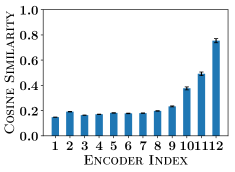
Figure 2: Cosine similarity for BERT encoders on the SST-2 dataset. The $j^{th}$ bar represents cosine similarity for the $j^{th}$ encoder, averaged over all pairs of word-vectors and all inputs.

The core intuition behind PoWER-BERT is that the redundancy of the word-vectors cannot possibly manifest abruptly at the last layer, rather must build progressively through the encoder pipeline. Consequently, we should be able to eliminate word-vectors in a progressive manner across all the encoders.

PoWER-BERT Components.

The PoWER-BERT scheme involves two critical, inter-related tasks. First, we identify a retention configuration: a monotonically decreasing sequence $(\ell_{1},\ell_{2},\ldots,\ell_{12})$ that specifies the number of word-vectors $\ell_{j}$ to retain at encoder $j$. For example, in Figure 1, the configuration is $(80,73,70,50,50,40,33,27,20,15,13,3)$. Secondly, we do word-vector selection, i.e., for a given input, determine which $\ell_{j}$ word-vectors to retain at each encoder $j$. We first address the task of word-vector selection.

3.2 Word-vector Selection

Assume that we are given a retention configuration $(\ell_{1},\ell_{2},\ldots,\ell_{12})$. Consider an encoder $j\in[1,12]$. The input to the encoder is a collection of $\ell_{j-1}$ word-vectors arranged in the form of a matrix of size $\ell_{j-1}\times 768$ (taking $\ell_{0}=N$). Our aim is to select $\ell_{j}$ word-vectors to retain and we consider two kinds of strategies.

Static and Dynamic Strategies.

Static strategies fix $\ell_{j}$ positions and retain the word-vectors at the same positions across all the input sequences in the dataset. A natural static strategy is to retain the first (or head) $\ell_{j}$ word-vectors. The intuition is that the input sequences are of varying lengths and an uniform length of $N$ is achieved by adding PAD tokens that carry little information. The strategy aims to remove as many PAD tokens on the average as possible, even though actual word-vectors may also get eliminated. A related method is to fix $\ell_{j}$ positions at random and retain word-vectors only at those positions across the dataset. We denote these strategies as Head-WS and Rand-WS, respectively (head/random word-vector selection).

In contrast to the static strategies, the dynamic strategies select the positions on a per-input basis. While the word-vectors tend to carry similar information at the final encoders, in the earlier encoders, they have different levels of influence over the final prediction. The positions of the significant word-vectors vary across the dataset. Hence, it is a better idea to select the positions for each input independently, as confirmed by our experimental evaluation.

We develop a scoring mechanism for estimating the significance of the word-vectors satisfying the following criterion: the score of a word-vector must be positively correlated with its influence on the final classification output (namely, word-vectors of higher influence get higher score). We accomplish the task by utilizing the self-attention mechanism and design a dynamic strategy, denoted as Attn-WS.

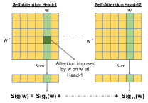
Figure 3: Figure shows significance score computation for word-vector $w$ using the computed self-attention matrix.

Attention-based Scoring.

Consider an encoder $j$ . In the PoWER-BERT setting, the input matrix $\mathbf{M}$ is of size $\ell_{j-1}\times 768$ and the attention matrices are of size $\ell_{j-1}\times\ell_{j-1}$. Consider an attention head $h\in[1,12]$. For a word $w^{\prime}$, the row $\mathbf{Z}_{h}[w^{\prime},:]$ computed by the head $h$ can be written as $\sum_{w}\mathbf{A}_{h}[w^{\prime},w]\cdot\mathbf{V}_{h}[w,:]$. In other words, the row $\mathbf{Z}_{h}[w^{\prime},:]$ is the weighted average of the rows of $\mathbf{V}_{h}$, taking the attention values as weights. Intuitively, we interpret the entry $\mathbf{A}_{h}[w^{\prime},w]$ as the attention received by word $w^{\prime}$ from $w$ on head $h$.

Our scoring function is based on the intuition that the significance of a word-vector $w$ can be estimated from the attention imposed by $w$ on the other word-vectors. For a word-vector $w$ and a head $h$, we define the significance score of $w$ for $h$ as ${\tt Sig}_{h}(w)=\sum_{w^{\prime}}\mathbf{A}_{h}[w^{\prime},w]$. The overall significance score of $w$ is then defined as the aggregate over the heads: ${\tt Sig}(w)=\sum_{h}{\tt Sig}_{h}(w)$. Thus, the significance score is the total amount of attention imposed by $w$ on the other words. See Figure 3 for an illustration.

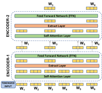
Figure 4: Word-vector selection over the first two encoders. Here, $N=6$, $\ell_{1}=4$ and $\ell_{2}=2$. The first encoder eliminates two word-vectors $w_{2}$ and $w_{4}$ with least significance scores; the second encoder further eliminates word-vectors $w_{1}$ and $w_{5}$.

Word-vector Extraction.

Given the scoring mechanism, we perform word-vector selection by inserting an extract layer between the self-attention module and the feed forward network. The layer computes the scores and retains the top $\ell_{j}$ word-vectors. See Figure 4 for an illustration.

Validation of the Scoring Function.

We conducted a study to validate the scoring function. We utilized mutual information to analyze the effect of eliminating a single word-vector. The study showed that higher the score of the eliminated word-vector, lower the agreement with the baseline model. Thus, the scoring function satisfies the criterion we had aimed for: the score of a word-vector is positively correlated with its influence on the final prediction. A detailed description of the study is deferred to the supplementary material.

PoWER-BERT uses a scoring mechanism for estimating the significance of the word-vectors satisfying the following criterion: the score of a word-vector must be positively correlated with its influence on the final classification output (namely, word-vectors of higher influence get higher score).

For a word-vector $w$ and a head $h$, we define the significance score of $w$ for $h$ as ${\tt Sig}_{h}(w)=\sum_{w^{\prime}}\mathbf{A}_{h}[w^{\prime},w]$ where $A_{h}$ is the attention matrix for head $h$ and $w^{\prime}$ signifies other words in the input sequence. The overall significance score of $w$ is then defined as the aggregate over the heads: ${\tt Sig}(w)=\sum_{h}{\tt Sig}_{h}(w)$.

We validate the scoring function using the well-known concept of mutual information and show that the significance score of a word is positively correlated with the classification output. Let $\mathbf{X}$ and $\mathbf{Y}$ be two random variables. Recall that the mutual information between $\mathbf{X}$ and $\mathbf{Y}$ is defined as $\mathbf{MI}(\mathbf{X};\mathbf{Y})=\mathbf{H}(\mathbf{X})-\mathbf{H}(\mathbf{X}|\mathbf{Y})$, where $\mathbf{H}(\mathbf{X})$ is the entropy of $\mathbf{X}$ and $\mathbf{H}(\mathbf{X}|\mathbf{Y})$ is the conditional entropy of $\mathbf{X}$ given $\mathbf{Y}$. The quantity is symmetric with respect to the two variables. Intuitively, Mutual information measure how much $\mathbf{X}$ and $\mathbf{Y}$ agree with each other. It quantifies the information that can be gained about $\mathbf{X}$ from information about $\mathbf{Y}$. If $\mathbf{X}$ and $\mathbf{Y}$ are independent random variables, then $\mathbf{MI}(\mathbf{X};\mathbf{Y})=0$. On the other hand, if the value of one variable can be determined with certainty given the value of the other, then $\mathbf{MI}(\mathbf{X};\mathbf{Y})=\mathbf{H}(\mathbf{X})=\mathbf{H}(\mathbf{Y})$.

Figure 5: Demonstration of mutual information

For this demonstration, we consider the SST-2 dataset from our experimental study with input length $N=128$ and number of classification categories $C=2$ (binary classification). Consider an encoder $j$ and we shall measure the mutual information between the classification output of the original model and a modified model that eliminates a single word at encoder $j$. Consider the trained BERT model without any word elimination and let $\mathbf{X}$ denote the classification label output by the model on a randomly chosen input from the training data. Fix an integer $k\leq\ell_{j-1}$ and let $w$ be the word with the $k^{th}$ highest significance score. Consider a modified model that does not eliminate any words on encoders $1,2,\ldots,j-1$, eliminates $w$ at encoder $j$, and does not eliminate any further words at encoders $j+1,j+2,\ldots,12$. Let $\mathbf{Y}_{k}$ be the random variable that denotes the classification output of the above model on a randomly chosen input. The mutual information between $\mathbf{X}$ and $\mathbf{Y}_{k}$ can be computed using the formula:

$$\sum_{b,b^{\prime}\in\{0,1\}}\Pr(\mathbf{X}=b,\mathbf{Y}=b^{\prime})\cdot\ln\left[\frac{\Pr(\mathbf{X}=b,\mathbf{Y}=b^{\prime})}{\Pr(\mathbf{X}=b)\cdot\Pr(\mathbf{Y}=b^{\prime})}\right]$$

We measured the mutual information between $\mathbf{X}$ and $\mathbf{Y}_{k}$ for all encoders $j$ and for all $k\in[1,128]$. Figure 5 shows the above data, wherein for the simplicity of presentation, we have restricted to encoders $j=1,3,6,9$. In this case, since the model predictions are approximately balanced between positive and negative, the baseline entropy is $\mathbf{H}(\mathbf{X})\sim\ln(2)=0.69$. We can make two observations from the figure. First is that as $k$ increases, the mutual information increases. This implies that deleting words with higher score results in higher loss of mutual information. Alternatively, deleting words with lower score results in higher mutual information, meaning the modified model gets in better agreement with the original model. Secondly, as the encoder number $j$ increases, the mutual information approaches the baseline entropy faster, confirming our hypothesis that words of higher significance scores (or more words) can be eliminated from the later encoders. The figure demonstrates that the score ${\tt Sig}(\cdot)$ captures the significance of the words in an effective manner.

3.3 Retention Configuration

We next address the task of determining the retention configuration. Analyzing all the possible configurations is untenable due to the exponential search space. Instead, we design a strategy that learns the retention configuration. Intuitively, we wish to retain the word-vectors with the topmost significance scores and the objective is to learn how many to retain. The topmost word-vectors may appear in arbitrary positions across different inputs in the dataset. Therefore, we sort them according to their significance scores. We shall learn the extent to which the sorted positions must be retained. We accomplish the task by introducing soft-extract layers and modifying the loss function.

Soft-extract Layer.

The extract layer either selects or eliminates a word-vector (based on scores). In contrast, the soft-extract layer would retain all the word-vectors, but to varying degrees as determined by their significance.

Consider an encoder $j$ and let $w_{1},w_{2},\ldots,w_{N}$ be the sequence of word-vectors input to the encoder. The significance score of $w_{i}$ is given by ${\tt Sig}(w_{i})$. Sort the word-vectors in the decreasing order of their scores. For a word-vector $w_{i}$, let ${\tt Sig}^{\it pos}(w_{i})$ denote the position of $w_{i}$ in the sorted order; we refer to it as the sorted position of $w_{i}$.

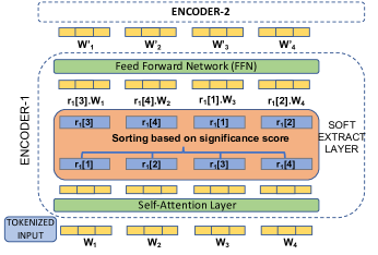
Figure 6: soft-extract layer. First encoder is shown, taking $N=4$. In this example, the sorted sequence of the word-vectors is $w_{3},w_{4},w_{1},w_{2}$; the most significant word-vector $w_{3}$ gets multiplied by ${\mathbf{r}}_{1}[1]$ and the least significant word-vector $w_{2}$ by ${\mathbf{r}}_{1}[4]$.

The soft-extract layer involves $N$ learnable parameters, denoted ${\mathbf{r}}_{j}[1],\ldots,{\mathbf{r}}_{j}[N]$, called retention parameters. The parameters are constrained to be in the range $[0,1]$. Intuitively, the parameter ${\mathbf{r}}_{j}[k]$ represents the extent to which the $k^{th}$ sorted position is retained.

The soft-extract layer is added in between the self-attention module and the feed forward network, and performs the following transformation. Let $\mathbf{E}^{in}$ denote the matrix of size $N\times 768$ output by the self-attention layer. For $i\in[1,N]$, the row $\mathbf{E}^{in}[i,:]$ yields the word-vector $w_{i}$. The layer multiplies the word-vector by the retention parameter corresponding to its sorted position:

$$\mathbf{E}^{out}[i,:]={\mathbf{r}}_{j}[{\tt Sig}^{\it pos}(w_{i})]\cdot\mathbf{E}^{in}[i,:].$$

The modified matrix $\mathbf{E}^{out}[i,:]$ is input to the feed-forward network. The transformation ensures that all the word-vectors in the $k^{th}$ sorted position get multiplied by the same parameter ${\mathbf{r}}_{j}[k]$. Figure 6 presents an illustration.

Loss Function.

We define the mass at encoder $j$ to be the extent to which the sorted positions are retained, i.e., ${{\rm mass}}(j;{\mathbf{r}})=\sum_{k=1}^{N}{\mathbf{r}}_{j}[k]$. Our aim is to minimize the aggregate mass over all the encoders with minimal loss in accuracy. Intuitively, the aggregate mass may be viewed as a budget on the total number of positions retained; ${\rm mass}(j;{\mathbf{r}})$ is the breakup across the encoders.

We modify the loss function by incorporating an $L_{1}$ regularizer over the aggregate mass. As demonstrated earlier, the encoders have varying influence on the classification output. We scale the mass of each encoder by its index. Let $\mathbf{\Theta}$ denote the parameters of the baseline BERT model and ${\cal L}(\cdot)$ be the loss function (such as cross entropy loss or mean-squared error) as defined in the original task. We define the new objective function as:

$$\min_{\mathbf{\Theta},{\mathbf{r}}}\left[{{\cal L}}(\mathbf{\Theta},{\mathbf{r}})~{}+~{}\lambda\cdot\sum_{j=1}^{L}j\cdot{\rm mass}(j;{\mathbf{r}})\right]$$

$${\rm s.t.}~{}~{}{\mathbf{r}}_{j}[k]\in[0,1]~{}~{}\forall(j\in[1,L],k\in[1,N]),$$

where $L$ is the number of encoders. While ${\cal L}(\mathbf{\Theta},{\mathbf{r}})$ controls the accuracy, the regularizer term controls the aggregate mass. The hyper-parameter $\lambda$ tunes the trade-off.

The retention parameters are initialized as ${\mathbf{r}}_{j}[k]=1$, meaning all the sorted positions are fully retained to start with. We train the model to learn the retention parameters. The learned parameter ${\mathbf{r}}_{j}[k]$ provides the extent to which the word-vectors at the $k^{th}$ sorted position must be retained. We obtain the retention configuration from the mass of the above parameters: for each encoder $j$, set $\ell_{j}={\tt ceil}({\rm mass}(j))$. In the rare case where the configuration is non-monotonic, we assign $\ell_{j}=\min\{\ell_{j},\ell_{j-1}\}$.

3.4 Training PoWER-BERT

Given a dataset, the scheme involves three training steps:

1. Fine-tuning: Start with the pre-trained BERT model and fine-tune it on the given dataset.

2. Configuration-search: Construct an auxiliary model by inserting the soft-extract layers in the fine tuned model, and modifying its loss function. The regularizer parameter $\lambda$ is tuned to derive the desired trade-off between accuracy and inference time. The model consists of parameters of the original BERT model and the newly introduced soft-extract layer. We use a higher learning rate for the latter. We train the model and derive the retention configuration.

3. Re-training: Substitute the soft-extract layer by extract layers. The number of word-vectors to retain at each encoder is determined by the retention configuration computed in the previous step. The word-vectors to be retained are selected based on their significance scores. We re-train the model.

In our experiments, all the three steps required only $2-3$ epochs. Inference is performed using the re-trained PoWER-BERT model. The CLS token is never eliminated and it is used to derive the final prediction.

Table 1: Dataset statistics: NLI and QA refers to Natural Language Inference and Question Answering tasks respectively. Note that STS-B is a regression task, therefore doesn’t have classes.

Dataset	Task	$\#$ Classes	Input Seq.
			Length $(N)$
CoLA	Acceptability	2	64
RTE	NLI	2	256
QQP	Similarity	2	128
MRPC	Paraphrase	2	128
SST-2	Sentiment	2	64
MNLI-m	NLI	3	128
MNLI-mm	NLI	3	128
QNLI	QA/NLI	2	128
STS-B	Similarity	-	64
IMDB	Sentiment	2	512
RACE	QA	2	512

Table 2: Comparison between PoWER-BERT and BERT_BASE. We limit the accuracy loss for PoWER-BERT to be within $1\%$ by tuning the regularizer parameter $\lambda$. Inference done on a K80 GPU with batch size of 128 (averaged over 100 runs). Matthew’s Correlation reported for CoLA; F1-score for QQP and MRPC; Spearman Correlation for STS-B; Accuracy for the rest.

	Method	CoLA	RTE	QQP	MRPC	SST-2	MNLI-m	MNLI-mm	QNLI	STS-B	IMDB	RACE
Test Accuracy	BERTBASE	52.5	68.1	71.2	88.7	93.0	84.6	84.0	91.0	85.8	93.5	66.9
	PoWER-BERT	52.3	67.4	70.2	88.1	92.1	83.8	83.1	90.1	85.1	92.5	66.0
Inference Time (ms)	BERTBASE	898	3993	1833	1798	905	1867	1881	1848	881	9110	20040
	PoWER-BERT	201	1189	405	674	374	725	908	916	448	3419	10110
Speedup		(4.5x)	(3.4x)	(4.5x)	(2.7x)	(2.4x)	(2.6x)	(2.1x)	(2.0x)	(2.0x)	(2.7x)	(2.0x)

Table 3: Comparison between PoWER-BERT and ALBERT. Here PoWER-BERT represents application of our scheme on ALBERT. The experimental setup is same as in Table 2

	Method	CoLA	RTE	QQP	MRPC	SST-2	MNLI-m	MNLI-mm	QNLI	STS-B
Test Accuracy	ALBERT	42.8	65.6	68.3	89.0	93.7	82.6	82.5	89.2	80.9
	PoWER-BERT	43.8	64.6	67.4	88.1	92.7	81.8	81.6	89.1	80.0
Inference Time (ms)	ALBERT	940	4210	1950	1957	922	1960	1981	1964	956
	PoWER-BERT	165	1778	287	813	442	589	922	1049	604
Speedup		(5.7x)	(2.4x)	(6.8x)	(2.4x)	(2.1x)	(3.3x)	(2.1x)	(1.9x)	(1.6x)

4 Experimental Evaluation

4.1 Setup

Datasets.

We evaluate our approach on a wide spectrum of classification/regression tasks pertaining to $9$ datasets from the GLUE benchmark Wang et al. (2019a), and the IMDB Maas et al. (2011) and the RACE Lai et al. (2017)) datasets. The datasets details are shown in Table 1.

Baseline methods.

We compare PoWER-BERT with the state-of-the-art inference time reduction methods: DistilBERT Sanh et al. (2019b), BERT-PKD Sun et al. (2019b) and Head-Prune Michel et al. (2019b). They operate by removing the parameters: the first two eliminate encoders, and the last prunes attention heads. Publicly available implementations were used for these methods Sanh et al. (2019a); Sun et al. (2019a); Michel et al. (2019a).

Hyper-parameters and Evaluation.

Training PoWER-BERT primarily involves four hyper-parameters, which we select from the ranges listed below: a) learning rate for the newly introduced soft-extract layers - $[10^{-4},10^{-2}]$; b) learning rate for the parameters from the original BERT model - $[2\times 10^{-5},6\times 10^{-5}]$; c) regularization parameter $\lambda$ that controls the trade-off between accuracy and inference time - $[10^{-4},10^{-3}]$; d) batch size - $\{4,8,16,32,64\}$. Hyper-parameters specific to the datasets are provided in the supplementary material.

The hyper-parameters for both PoWER-BERT and the baseline methods were tuned on the Dev dataset for GLUE and RACE tasks. For IMDB, we subdivided the training data into 80% for training and 20% for tuning. The test accuracy results for the GLUE datasets were obtained by submitting the predictions to the evaluation server , whereas for IMDB and RACE, the reported results are on the publicly available Test data.

Implementation.

The code for PoWER-BERT was implemented in Keras and is available at https://github.com/IBM/PoWER-BERT. The inference time experiments for PoWER-BERT and the baselines were conducted using Keras framework on a K80 GPU machine. A batch size of 128 (averaged over 100 runs) was used for all the datasets except RACE, for which the batch size was set to 32 (since each input question has 4 choices of answers).

Maximum Input Sequence Length.

The input sequences are of varying length and are padded to get a uniform length of $N$. Prior work use different values of $N$, for instance ALBERT uses $N=512$ for all GLUE datasets. However, only a small fraction of the inputs are of length close to the maximum. Large values of $N$ would offer easy pruning opportunities and larger gains for PoWER-BERT. To make the baselines competitive, we set stringent values of $N$: we determined the length $N^{\prime}$ such that at most $1\%$ of the input sequences are longer than $N^{\prime}$ and fixed $N$ to be the value from $\{64,128,256,512\}$ closest to $N^{\prime}$. Table 1 presents the lengths specific to each dataset.

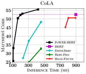
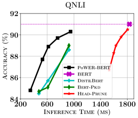
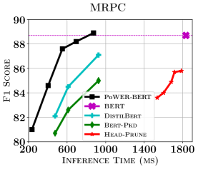
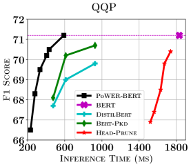
Figure 7: Comparison to prior methods. Pareto curves showing accuracy vs. inference time trade-off. Top-left corners correspond to the best inference time and accuracy. Points for PoWER-BERT obtained by tuning the regularizer parameter $\lambda$. For DistilBERT and BERT-PKD, the points correspond to retaining $\{3,4,6\}$ encoders. For Head-Prune, points obtained by varying number of retained attention-heads. The cross represents BERT_BASE performance; dotted line represents its accuracy (for the ease of comparison). Over the best baseline method, PoWER-BERT offers: accuracy gains as high as $16\%$ on CoLA and $6\%$ on RTE at inference time $305$ ms and $1326$ ms, respectively; inference time gains as high as $2.7$x on CoLA and $2$x on RTE at accuracy $48.2\%$ and $65.5\%$, respectively.

4.2 Evaluations

Comparison to BERT.

In the first experiment, we demonstrate the effectiveness of the word-vector elimination approach by evaluating the inference time gains achieved by PoWER-BERT over BERT_BASE. We limit the accuracy loss to be within $1\%$ by tuning the regularizer parameter $\lambda$ that controls the trade-off between inference time and accuracy. The results are shown in Table 2. We observe that PoWER-BERT offers at least $2.0$x reduction in inference time on all the datasets and the improvement can be as high as $4.5$x, as exhibited on the CoLA and the QQP datasets.

We present an illustrative analysis by considering the RTE dataset. The input sequence length for the dataset is $N=256$. Hence, across the twelve encoders, BERT_BASE needs to process $12\times 256=3072$ word-vectors for any input. In contrast, the retention configuration used by PoWER-BERT on this dataset happens to be $(153,125,111,105,85,80,72,48,35,27,22,5)$ summing to $868$. Thus, PoWER-BERT processes an aggregate of only $868$ word-vectors. The self-attention and the feed forward network modules of the encoders perform a fixed amount of computations for each word-vector. Consequently, the elimination of the word-vectors leads to reduction in computational load and improved inference time.

Comparison to Prior Methods.

In the next experiment, we compare PoWER-BERT with the state-of-the-art inference time reduction methods, by studying the trade-off between accuracy and inference time. The Pareto curves for six of the GLUE datasets are shown in Figure 7; others are provided in the supplementary material. Top-left corners correspond to the best inference time and accuracy.

For PoWER-BERT, the points on the curves were obtained by tuning the regularizer parameter $\lambda$. For the two encoder elimination methods, DistilBERT and BERT-PKD, we derived three points by retaining $3$, $4$, and $6$ encoders; these choices were made so as to achieve inference time gains comparable to PoWER-BERT. Similarly, for the Head-Prune strategy, the points were obtained by varying the number of attention-heads retained.

Figure 7 demonstrates that PoWER-BERT exhibits marked dominance over all the prior methods offering:

• Accuracy gains as high as $16\%$ on CoLA and $6\%$ on RTE for a given inference time.

• Inference time gains as high as $2.7$x on CoLA and $2.0$x on RTE for a given accuracy.

The results validate our hypothesis that fine-grained word-vector elimination yields better trade-off than coarse-grained encoder elimination. We also observe that Head-Prune is not competitive. The reason is that the method exclusively targets the attention-heads constituting only $~{}26\%$ of the BERT_BASE parameters and furthermore, pruning a large fraction of the heads would obliterate the critical self-attention mechanism of BERT.

Accelerating ALBERT.

As discussed earlier, word-vector elimination scheme can be applied over compressed models as well. To demonstrate, we apply PoWER-BERT over ALBERT, one of the best known compression methods for BERT. The results are shown in Table 3 for the GLUE datasets. We observe that the PoWER-BERT strategy is able to accelerate ALBERT inference by $2$x factors on most of the datasets (with $<1\%$ loss in accuracy), with the gain being as high as $6.8$x on the QQP dataset.

Table 4: Comparison of the accuracy of the word-vector selection methods on the SST-2 Dev set for a fixed retention configuration.

	Head-WS	Rand-WS	Attn-WS
Entire dataset	85.4%	85.7%	88.3%
Input sequence length $>16$	83.7%	83.4%	87.4%

Ablation Study.

In Section 3.2, we described three methods for word-vector selection: two static techniques, Head-WS and Rand-WS, and a dynamic strategy, denoted Attn-WS, based on the significance scores derived from the attention mechanism. We demonstrate the advantage of Attn-WS by taking the SST-2 dataset as an illustrative example. For all the three methods, we used the same sample retention configuration of $(64,32,16,16,16,16,16,16,16)$. The accuracy results are shown in Table 4. The first row of the table shows that Attn-WS offers improved accuracy. We perform a deeper analysis by filtering inputs based on length. In the given sample configuration, most encoders retain only $16$ word-vectors. Consequently, we selected a threshold of $16$ and considered a restricted dataset with inputs longer than the threshold. The second row shows the accuracy results.

Recall that Head-WS relies on eliminating as many PAD tokens as possible on the average. We find that the strategy fails on longer inputs, since many important word-vectors may get eliminated. Similarly, Rand-WS also performs poorly, since it is oblivious to the importance of the word-vectors. In contrast, Attn-WS achieves higher accuracy by carefully selecting word-vectors based on their significance. The inference time is the same for all the methods, as the same number of word-vectors get eliminated.

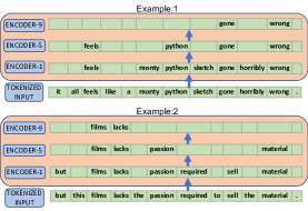
Figure 8: Anecdotal Examples. Real-life examples from SST-2 dataset demonstrating progressive word-vector elimination.

Anecdotal Examples.

We present real-life examples demonstrating word-vector redundancy and our word-vector selection strategy based on the self-attention mechanism (Attn-WS). For this purpose, we experimented with sentences from the SST-2 sentiment classification dataset and the results are shown in Figure 8.

Both the sentences have input sequence length $N=12$ (tokens). We set the retention configuration as $(7,7,7,7,4,4,4,4,2,2,2,2)$ so that it progressively removes five word-vectors at the first encoder, and two more at the fifth and the ninth encoders, each.

In both the examples, the first encoder eliminates the word-vectors corresponding to stop words and punctuation. The later encoders may seem to eliminate more relevant word-vectors. However, their information is captured by the word-vectors retained at the final encoder, due to the diffusion of information. These retained word-vectors carry the sentiment of the sentence and are sufficient for correct prediction. The above study further reinforces our premise that word-vector redundancy can be exploited to improve inference time, while maintaining accuracy.

5 Conclusions

We presented PoWER-BERT, a novel method for improving the inference time of the BERT model by exploiting word-vectors redundancy. Experiments on the standard GLUE benchmark show that PoWER-BERT achieves up to $4.5$x gain in inference time over BERT_BASE with $<1\%$ loss in accuracy. Compared to prior techniques, it offers significantly better trade-off between accuracy and inference time. We showed that our scheme can be applied over ALBERT, a highly compressed variant of BERT. For future work, we plan to extend PoWER-BERT to wider range of tasks such as language translation and text summarization.

References

- Correia et al. [2019] Gonçalo M. Correia, Vlad Niculae, and André F. T. Martins. Adaptively sparse transformers. Proceedings of the 2019 Conference on Empirical Methods in Natural Language Processing and the 9th International Joint Conference on Natural Language Processing (EMNLP-IJCNLP), 2019.
- Denil et al. [2013] Misha Denil, Babak Shakibi, Laurent Dinh, Marc’Aurelio Ranzato, and Nando De Freitas. Predicting parameters in deep learning. In NIPS, 2013.
- Devlin et al. [2019] Jacob Devlin, Ming-Wei Chang, Kenton Lee, and Kristina Toutanova. BERT: Pre-training of deep bidirectional transformers for language understanding. In NAACL, 2019.
- Gong et al. [2014] Yunchao Gong, Liu Liu, Ming Yang, and Lubomir Bourdev. Compressing deep convolutional networks using vector quantization. arXiv preprint arXiv:1412.6115, 2014.
- Han et al. [2015] Song Han, Jeff Pool, John Tran, and William Dally. Learning both weights and connections for efficient neural network. In NIPS, 2015.
- He et al. [2017] Yihui He, Xiangyu Zhang, and Jian Sun. Channel pruning for accelerating very deep neural networks. In ICCV, 2017.
- Hinton et al. [2015] Geoffrey Hinton, Oriol Vinyals, and Jeff Dean. Distilling the knowledge in a neural network. arxiv preprint: 1503.02531, 2015.
- Kim et al. [2015] Yong-Deok Kim, Eunhyeok Park, Sungjoo Yoo, Taelim Choi, Lu Yang, and Dongjun Shin. Compression of deep convolutional neural networks for fast and low power mobile applications. arxiv preprint: 1511.06530, 2015.
- Lai et al. [2017] Guokun Lai, Qizhe Xie, Hanxiao Liu, Yiming Yang, and Eduard Hovy. Race: Large-scale reading comprehension dataset from examinations. arXiv preprint arXiv:1704.04683, 2017.
- Lan et al. [2019] Zhenzhong Lan, Mingda Chen, Sebastian Goodman, Kevin Gimpel, Piyush Sharma, and Radu Soricut. ALBERT: A lite BERT for self-supervised learning of language representations. arXiv preprint arXiv:1909.11942, 2019.
- Lee et al. [2019] Jinhyuk Lee, Wonjin Yoon, Sungdong Kim, Donghyeon Kim, Sunkyu Kim, Chan Ho So, and Jaewoo Kang. BioBERT: Pre-trained biomedical language representation model for biomedical text mining. Bioinformatics, 2019.
- Liu and Lapata [2019] Yang Liu and Mirella Lapata. Text summarization with pretrained encoders. arXiv preprint arXiv:1908.08345, 2019.
- Liu et al. [2019] Xiaodong Liu, Pengcheng He, Weizhu Chen, and Jianfeng Gao. Improving multi-task deep neural networks via knowledge distillation for natural language understanding. arxiv preprint: 1904.09482, 2019.
- Maas et al. [2011] Andrew L. Maas, Raymond E. Daly, Peter T. Pham, Dan Huang, Andrew Y. Ng, and Christopher Potts. Learning word vectors for sentiment analysis. In ACL, 2011.
- Martins and Astudillo [2016] André F. T. Martins and Ramón Fernandez Astudillo. From softmax to sparsemax: A sparse model of attention and multi-label classification. 2016.
- McCarley [2019] J. S. McCarley. Pruning a BERT-based question answering model. arxiv preprint: 1910.06360, 2019.
- Michel et al. [2019a] Paul Michel, Omer Levy, and Graham Neubig, 2019.
- Michel et al. [2019b] Paul Michel, Omer Levy, and Graham Neubig. Are sixteen heads really better than one? arXiv preprint arXiv:1905.10650, 2019.
- Molchanov et al. [2016] Pavlo Molchanov, Stephen Tyree, Tero Karras, Timo Aila, and Jan Kautz. Pruning convolutional neural networks for resource efficient inference. arxiv preprint: 1611.06440, 2016.
- Molchanov et al. [2017] Dmitry Molchanov, Arsenii Ashukha, and Dmitry Vetrov. Variational dropout sparsifies deep neural networks. arxiv preprint: 1701.05369, 2017.
- Peters et al. [2019] Ben Peters, Vlad Niculae, and André F. T. Martins. Sparse sequence-to-sequence models. Proceedings of the 57th Annual Meeting of the Association for Computational Linguistics, 2019.
- Rajpurkar et al. [2016] Pranav Rajpurkar, Jian Zhang, Konstantin Lopyrev, and Percy Liang. SQuAD: 100,000+ questions for machine comprehension of text. arXiv preprint arXiv:1606.05250, 2016.
- Sanh et al. [2019a] Victor Sanh, Lysandre Debut, Julien Chaumond, and Thomas Wolf, 2019.
- Sanh et al. [2019b] Victor Sanh, Lysandre Debut, Julien Chaumond, and Thomas Wolf. DistilBERT, a distilled version of BERT: smaller, faster, cheaper and lighter. arXiv preprint arXiv:1910.01108, 2019.
- Sau and Balasubramanian [2016] Bharat Bhusan Sau and Vineeth N. Balasubramanian. Deep model compression: Distilling knowledge from noisy teachers. arxiv preprint: 1610.09650, 2016.
- Shen et al. [2019] Sheng Shen, Zhen Dong, Jiayu Ye, Linjian Ma, Zhewei Yao, Amir Gholami, Michael W. Mahoney, and Kurt Keutzer. Q-BERT: Hessian based ultra low precision quantization of BERT. arxiv preprint:1909.05840, 2019.
- Sun et al. [2019a] Siqi Sun, Yu Cheng, Zhe Gan, and Jingjing Liu, 2019.
- Sun et al. [2019b] Siqi Sun, Yu Cheng, Zhe Gan, and Jingjing Liu. Patient knowledge distillation for BERT model compression. arXiv preprint arXiv:1908.09355, 2019.
- Wang et al. [2019a] Alex Wang, Amanpreet Singh, Julian Michael, Felix Hill, Omer Levy, and Samuel R. Bowman. GLUE: A multi-task benchmark and analysis platform for natural language understanding. In ICLR, 2019.
- Wang et al. [2019b] Ziheng Wang, Jeremy Wohlwend, and Tao Lei. Structured pruning of large language models. arxiv preprint: 1910.04732, 2019.
- Zafrir et al. [2019] Ofir Zafrir, Guy Boudoukh, Peter Izsak, and Moshe Wasserblat. Q8BERT: Quantized 8bit BERT. arxiv preprint:1910.06188, 2019.
- Zhao et al. [2019] Guangxiang Zhao, Junyang Lin, Zhiyuan Zhang, Xuancheng Ren, Qi Su, and Xu Sun. Explicit sparse transformer: Concentrated attention through explicit selection. arXiv,1912.11637, 2019.